Discreteness effects on the fluxon interaction with the dipole impurity in the Josephson transmission line

Abstract

The influence of discreteness on the fluxon scattering on the dipole-like impurity is studied. This kind of impurity is used to model the qubit inductively coupled to the Josephson transmission line (JTL). The previously proposed fluxon assisted readout process of the qubit state is based on measuring the passage time through the dipole impurity. The aim of this work is to clarify the role of the discreteness in this qubit readout process. It is demonstrated that the fluxon delay time on the qubit impurity increases significantly if the discreteness of the JTL increases. Also it is shown that the difference between the fluxon threshold currents for the positive and negative qubits decreases with the increase of discreteness.

1 Introduction

The Josephson effect is among the the most remarkable phenomena in physics of superconductors [1, 2]. Spatially extended systems that consist of Josephson junctions (JJs) have been an important area of scientific research during the last decades. One of the reasons for this activity is the abundance of various nontrivial nonlinear phenomena observed in such systems and their applications such as topological soliton (fluxon) [3, 4, 5] and discrete breather [6, 7] observation, dynamical chaos [8, 9], metastructures [10], metrological applications [11] to name a few.

One of the important application of fluxons in Josephson junctions is quantum computation [12]-[20]. The qubit readout process suggested in [13] and studied further both analytically and experimentally in [14]-[18],[21] is based on the Josephson transmission line inductively coupled to a qubit. The fluxon (Josephson vortex) is launched at the JTL end, and, since its interaction with the $|0\rangle$ and $|1\rangle$ qubit states takes different times, its arrival at the opposite JTL end occurs after different time intervals. Hence, by measuring the delay time one can determine the state of the qubit.

It should be noted that although the JTL are discrete, all the theoretical research on the fluxon qubit readout [13, 14, 18, 21] has been performed in the continuum approximation. Therefore it is natural to investigate the role of discreteness in the qubit readout process in JTLs. Topological soliton interaction with spatial inhomogeneities has been studied rather well [22, 23], however, the case of an dipole inhomogeneity in the discrete media requires much more attention.

The main goal of this work is to investigate the effect of discreteness on the qubit readout and to find a way to maximize the sensitivity of the qubit readout process.

This paper is organized as follows. In the next Section we describe the model. In Sec. 3 the main results on the fluxon transmission are presented and the threshold current is computed. In Sec. 4 the fluxon delay time on the qubit is obtained. Discussion and conclusions are given in the last Section.

2 The model

We consider the Josephson junction array or, in other words, the Josephson transmission line (JTL) and a qubit coupled inductively to it. The Hamiltonian of the JTL interacting with the qubit can be written [13, 14] as follows:

$$H = \sum_{n=1}^{N}\left[\frac{Q_{n}^{2}}{2C}+E_{J}(1-\cos\phi_{n})+\right.$$ (1)

$$+ \left.\frac{1}{2L}\left(\frac{\Phi_{0}}{2\pi}\right)^{2}(\phi_{n+1}-\phi_{n}-\phi_{n}^{(e)})^{2}\right].$$

Here the charge on the $n$th junction equals $Q_{n}=C\hbar\dot{\phi}_{n}/(2e)$, the Josephson coupling energy $E_{J}=\hbar I_{c}/(2e)$. Each junction is described by the Josephson phase $\phi_{n}$ which is the difference of the wavefunction phases for each of the superconducting electrodes that form the junction. The flux induced by the qubit will be denoted as $\Phi_{n}^{(e)}={\Phi_{0}}\phi_{n}^{(e)}/(2\pi)$, $L$ is selfinductance of the JTL cell, $I_{c}$ is the junction critical current and $\Phi_{0}$ is magnetic flux quantum.

The equations of motion for the Josephson phase can be obtained in the standard way from the Hamiltonian (1). They must be complemented by the dissipative term that describes the normal electron current $\hbar\dot{\phi}_{n}/(2eR)$ across the junction with $R$ being the resistance of an individual junction. The external dc bias $I_{B}$ is applied to each junction. Hence, the equations of motion read

$$\frac{C\hbar}{2e}\ddot{\phi}_{n}+\frac{\hbar}{2eR}\dot{\phi}_{n}+I_{c}\sin\phi_{n}-$$ (2)

$$-\frac{\Phi_{0}}{2\pi L}\hat{\Delta}\phi_{n}=I_{B}+\frac{\Phi_{0}}{2\pi L}\left(\phi_{n}^{(e)}-\phi_{n-1}^{(e)}\right),$$

$$\hat{\Delta}\phi_{n}\equiv\phi_{n+1}-2\phi_{n}+\phi_{n-1},\;\ n=\overline{1,N}.$$

Throughout the paper only the linear JTLs are to be described, therefore the open ends boundary conditions will be used. It is convenient to introduce the dimensionless variables

$$H\to\frac{H}{E_{J}};~{}t\to t\omega_{J},\omega_{J}=\sqrt{\frac{C\hbar}{2eI_{c}}};$$ (3)

$$~{}\gamma=\frac{I_{B}}{I_{c}};~{}\kappa=\frac{\Phi_{0}}{2\pi LI_{c}}.$$

As a result a dimensionless damped and dc driven discrete sine-Gordon (DSG) equation is obtained:

$$\ddot{\phi}_{n}+\alpha\dot{\phi}_{n}+\sin\phi_{n}-\kappa\hat{\Delta}\phi_{n}=$$ (4)

$$=\gamma+f_{n},~{}n=\overline{1,N},$$

where $\gamma$ denotes the dimensionless bias current and the constant $\kappa$ is the measure of the discreteness. When $\kappa$ decreases the discreteness effects become stronger. In the opposite limit $\kappa\to\infty$ they disappear and the continuum limit is restored. The spatially inhomogeneous term $f_{n}$ is written in the following form

$$f_{n}=\frac{\Phi_{0}}{2\pi LI_{c}}\left(\phi_{n}^{(e)}-\phi_{n-1}^{(e)}\right)=$$

$$=\frac{1}{LI_{c}}\left(\Phi_{n}^{(e)}-\Phi_{n-1}^{(e)}\right)=$$

$$=\sigma\kappa\left\{\begin{array}[]{ccc}0&,&n\neq n_{0}-1,~{}n_{0},\\ |\mu|&,&n=n_{0}-1,\\ -|\mu|&,&n=n_{0}.\end{array}\right.$$ (8)

Here $\sigma=\mbox{sign}\mu=\pm 1$ is the qubit polarity, which defines its state, the parameter $\kappa\mu$ measures the strength of the impurity and equals

$$\kappa\mu=\frac{\kappa}{\kappa_{q}}=\frac{L_{q}I_{q}}{LI_{c}},\;\;\kappa_{q}=\frac{\Phi_{0}}{2\pi L_{q}I_{q}},$$ (9)

Here $I_{q}$ is the current in the qubit cirquit. The total dimensionless energy reads

$$E=E_{k}+E_{p},\;E_{k}=\frac{1}{2}\sum_{n=1}^{N}\dot{\phi}^{2}_{n},$$ (10)

$$E_{p}=\sum_{n=1}^{N}\left[\frac{\kappa(\phi_{n+1}-\phi_{n})^{2}}{2}+\right.$$ (11)

$$\left.+2\sin^{2}{\frac{\phi_{n}}{2}}+(\gamma+f_{n})\phi_{n}\right].$$

In the following sections we will analyze both analytically and numerically fluxon interaction with the qubit.

3 Fluxon transmission through the qubit and the threshold current.

3.1 General remarks about topological soliton interactions with impurities

The problem of topological soliton interaction with spatial inhomogeneities in both the continuous and discrete systems has been studied thoroughly during the several last decades (see the respective chapters in the reviews and books [24, 25, 27]). It is useful to recall several important facts. Generally speaking, solitons can get pinned by the inhomogeneity whenever it is lattice discreteness or just an individual impurity. If the system has dissipation and is biased by the constant current, the most typical situation consists of the following scenarios:

• $0<\gamma<\gamma_{thr}$. In this case the inhomogeneity is so strong that a soliton cannot pass it. The value $\gamma_{thr}$ is known as the threshold current. It is the minimal current for which a soliton can propagate.

• $\gamma_{thr}<\gamma<\gamma_{c}$. The bias is strong enough to sustain moving solitons. Both moving and standing (pinned by the inhomogeneity) solitons can exist. Depending on the initial condition the system can settle on any of these states.

• $\gamma>\gamma_{c}$. Bias is so strong that impurities cannot trap the soliton.

Discreteness obstructs free soliton propagation along the array. There exists a critical depinning current $\gamma_{PN}$ such that for $\gamma<\gamma_{PN}$ no soliton propagation is possible. If $\kappa$ is too small the soliton cannot move. We will consider only the values of $\kappa$ large enough that $\gamma_{PN}<\gamma_{thr}$.

3.2 Manifestation of the discreteness effects

In this subsection we will compute numerically the threshold current $\gamma_{thr}^{\pm}=\gamma_{thr}(\sigma=\pm 1)$ for the impurities with the different polarities $\sigma$. For the numerical simulations of the DSG equation (4) the 4th order Runge-Kutta method will be used. The details of the fluxon interaction with the dipole impurity are given in Fig. 1, the threshold current as a function of the system parameters is given in Figs. 2-3. In this subsection the JTL size is chosen to be large enough ($N=300\div 600$) to avoid any boundary effects. A special case of short JTLs is discussed separately in Subsec. 4.2.

Fluxon transmission through a lattice inhomogeneity has certain principal differences from the respective continuum case. This is illustrated by the time dependencies of the total kinetic energy of the JTL (10) for the different values of the discreteness constant $\kappa$ and external bias $\gamma$. The bias was chosen to be slightly higher than the respective threshold value $\gamma^{\pm}_{thr}$. These dependencies are presented in Fig. 1. The fluxon dynamics in the vicinity of the qubit impurity depends on the impurity polarity. For the positive polarity ($\sigma=1$), the fluxon slows down before approaching the qubit and accelerates back to its equilibrium velocity.

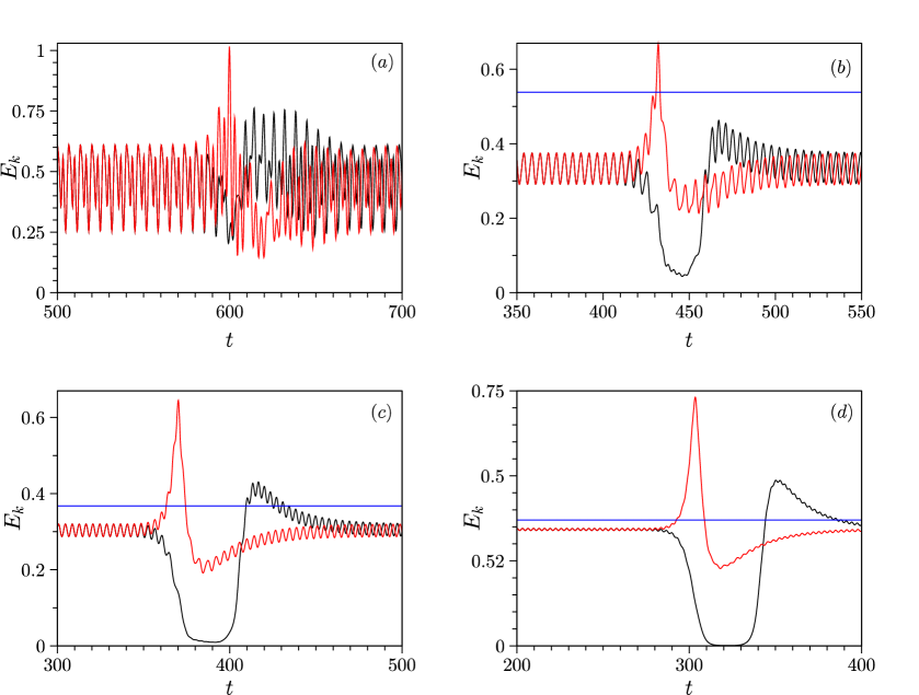
Figure 1: (Colour online.) Total kinetic energy (10) as a function of time for the fluxon interacting with the qubit ($\sigma=1$, black and $\sigma=-1$, red) for $\kappa=0.5$, $\gamma=0.0487$ (a), $\kappa=0.75$, $\gamma=0.0251$ (b), $\kappa=1$, $\gamma=0.0193$ (c) and $\kappa=1.5$, $\gamma=0.0175$ (d). Other parameters are: $\alpha=0.05$ and $|\mu|=0.2$. Solid blue line corresponds to the fluxon kinetic energy in the continuum case $E_{k}=4\sqrt{\kappa}v^{2}_{\infty}$.

For the $\sigma=-1$ the situation is the opposite. The fluxon accelerates first and then slows down back to the equilibrium velocity. This is consistent with the continuum approximation [21, 26] in which the $\sigma=1$ impurity is felt by the fluxon as a potential barrier. On the contrary, the fluxon sees the $\sigma=-1$ impurity as a potential well. Another useful observation is the amplitude of the kinetic energy oscillations. These oscillations appear due to discreteness and are rather weak even for the sufficiently discrete JTL with $\kappa=1.5$ (see Fig. 1d). As the discreteness increases, these oscillations increase as well, eventually reaching the situation when they are of the order of the average kinetic energy value (see Fig. 1a). This means that the contribution of the oscillations around the fluxon center of mass is very strong.

If discreteness is weak ($\kappa\gg 1$), it is possible to project the many-body problem described by the DSG equation (4) onto the two-dimensional subspace of the collective coordinates $(X,v)$ where $X=X(t)$ it the fluxon center of mass and $v(t)$ is its velocity. The discreteness of the media is modelled by the Peierls-Nabarro (PN) potential. Using the technique described in [23, 27] one arrives to the collective equations of motion on the fluxon center of mass $X$, $\phi(x,t)\approx 4\tan^{-1}\exp{[x-X(t)]}$, $x\approx nh$, $h=1/\sqrt{\kappa}$:

$$8\ddot{X}+8\alpha\dot{X}=-\frac{\partial U}{\partial X}=$$

$$=-\frac{\partial}{\partial X}\left[U_{0}(X)+U_{\gamma}(X)+U_{PN}(X)\right].$$ (12)

This is a newtonian equation of motion for the dissipative particle with the mass $m=8$ in the field created by the potential $U(X)$. This potential consists of three parts. The first one, $U_{0}(X)$ is created by the impurity, the second one, $U_{\gamma}(X)$, appears due to the external bias. The last one is the PN potential $U_{PN}(X)$. The explicit form of these potentials is written as follows:

$$U_{PN}(X)=\Delta_{PN}\cos(2\pi\sqrt{\kappa}X),$$ (13)

$$\Delta_{PN}=\frac{16\pi^{2}\sqrt{\kappa}}{\sinh(\pi^{2}\sqrt{\kappa})},$$ (14)

$$U_{0}(X)=\frac{2\mu\sigma}{\cosh{X}},$$ (15)

$$U_{\gamma}(X)=-2\pi\gamma X-\frac{2\gamma}{\sqrt{\kappa}}\frac{\sin(2\pi X\sqrt{\kappa})}{\cosh(\pi^{2}\sqrt{\kappa})}.$$ (16)

It appears that the potential $U_{0}(X)$ does not depend on discreteness.

In the continuum limit ($x\approx nh$) the DSG equation (4-8) transforms into continuous sine-Gordon (SG) equation

$$\phi_{tt}-\phi_{xx}+\sin\phi+\alpha\phi_{t}=$$ (17)

$$=\sigma|\mu|\delta^{\prime}(x)+\gamma,\;$$

which has been studied previously [14, 21, 26]. In the continuum limit the collective-coordinate equations (12)-(16) will contain only the potentials $U_{0}(X)$ and $U_{\gamma}(X)=-2\pi\gamma X$. The PN potential will naturally be absent. As a result, the approach developed in papers [21, 28] can be applied. Thus, the threshold currents are given by (see Ref. [21] for details):

$$\gamma_{thr,c}^{+}={\Upsilon}^{+}_{1}\alpha+\Upsilon_{2}^{+}\alpha^{2}=$$

$$=\frac{2\sqrt{{2\mu}}}{\pi}\alpha-\frac{8}{\pi}\ln\left(\frac{1+\sqrt{2}}{\sqrt{2}}\right)\alpha^{2}~{},$$ (18)

$$\gamma_{thr,c}^{-}=\frac{4\Gamma\left(\frac{1}{4}\right)}{\pi^{5/4}}\left|{\mu}\right|^{1/4}\alpha^{3/2}+$$

$$+12\frac{\alpha^{2}}{\pi}\ln\left[\left(\frac{2\Gamma\left(\frac{1}{4}\right)}{\pi^{1/4}}\right)^{2/3}\frac{\alpha}{\sqrt{|\mu|}}\right]~{}.$$ (19)

In the positive polarity case the first term $\Upsilon_{1}^{+}\alpha$ can be obtained from the kinematic approach [29]. The second term $\Upsilon^{+}_{2}\alpha^{2}$ is a correction that requires more elaborate approximation [28]. The ${\cal O}(\alpha)$ term is sufficient to have the crudest approximation. The kinematic approximation states that the threshold current is found from the condition that the total fluxon kinetic energy is spent to overcome the qubit-created potential. For the positive polarity $\sigma=1$ this means $E_{k}=4v^{2}_{\infty}=U(X_{max})-U(X_{min})$. If we assume that the incoming fluxon velocity is small and does not differ significantly from its continuum value, we can use $v_{\infty}\approx\pi\gamma/(4\alpha)$. The potential barrier $U(X_{max})-U(X_{min})$ must contain two contributions: the height of the impurity potential $2\mu$ [see Eq. (15)] and the height of the PN potential $2\Delta_{PN}$ [see Eq. (16)]. As a result we obtain the first order approximation to the threshold current in JTL

$$\gamma^{+}_{thr,1}=\frac{4\alpha}{\pi}\sqrt{\frac{\mu+\Delta_{PN}}{2}},$$ (20)

where the PN barrier amplitude $\Delta_{PN}$ is given in Eq. (14). In Fig. 2 the numerically calculated dependencies $\gamma^{\pm}_{thr}(\kappa)$ are shown. Solid lines correspond to the numerically computed data. Dashed lines represent analytical approximations. In the continuum limit ($\kappa\to\infty$) the dependencies for both qubit polarities become flat.

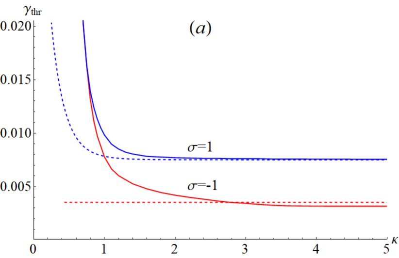
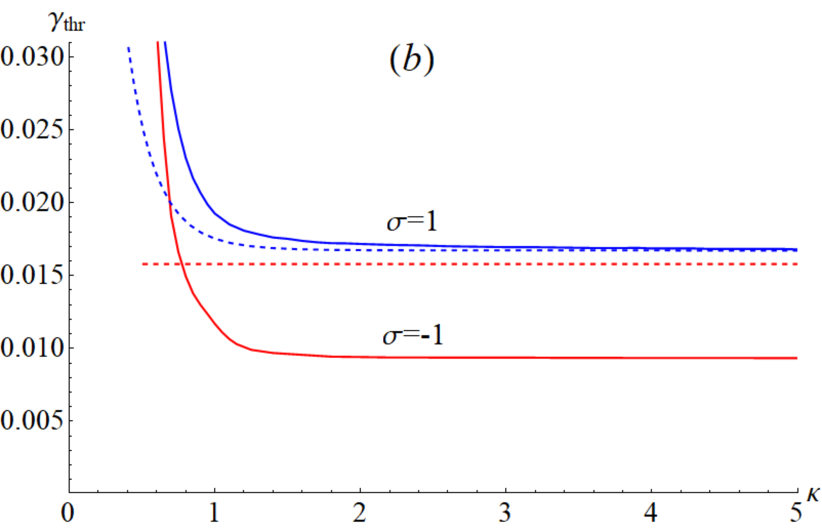
Figure 2: (Colour online.) Threshold current as a function of the discreteness parameter for $|\mu|=0.2$ and $\alpha=0.02$ (a) and $\alpha=0.05$ (b). Red colour corresponds to $\sigma=-1$ and blue line is $\sigma=1$. Solid lines correspond to the numerically computed results, dashed line is analytical approximation (see text for details).

The threshold currents for both $\sigma=1$ and $\sigma=-1$ qubits increase strongly with the increase of discreteness. This is quite natural because the fluxon needs more energy to overcome not only the impurity potential but the PN potential as well. Another important point is that the difference $\gamma^{+}_{thr}-\gamma^{-}_{thr}$ decreases as $\kappa\to 0$. This can be explained by the fact that the obstructive influence of discreteness is so strong that it does not discriminate between different polarities of the qubit. In other words, the influence of the PN potential is of the same order as of the impurity potential. This situation is illustrated quite clearly in Fig. 1d, where the time oscillations of the kinetic energy due to the PN barrier are of the same order as the kinetic energy itself. At some value of $\kappa$ the dependencies coincide, however, we did not follow them to very small values because of difficulty in defining $\gamma_{thr}$. This point will be discussed below. For the $\sigma=+1$ case the continuum limit (18) is restored with high accuracy. In order to compare our numerical results with the continuum limit, we have plotted the combined approximation $\gamma^{+}_{thr}(\alpha)=\gamma^{+}_{thr,1}(\alpha)+\Upsilon_{2}^{+}\alpha^{2}$ where the first term comes from the kinematic approximation (20) and the second one is the second term from the continuum limit correction (18). The abovementioned analytical approximation captures the main features of the $\gamma_{thr}(\kappa)$ dependence but is not that accurate for $\kappa\sim 1$. This means that the collective- coordinate PN approximation (12)-(16) does not work well for strongly discrete lattices. In the case of $\sigma=-1$ we have plotted only the continuum approximation (dashed red line) of the threshold current (19) because the analytical approximation appears to be highly complicated. One can observe that the coincidence between the numerical and analytical results in the continuum limit varies. The answer lies in the fact that the validity of the approximation, which allows to obtain Eq. (20), is limited. For details one can consult Ref. [21]. The approximation (20) is obtained under the assumptions $\alpha\ll|\mu|\ll 1$, $\gamma\ll|\mu|\ll 1$, and $\alpha\ll\sqrt{|\mu|/2}$. In the case $\alpha=0.05$ the last inequality is fulfilled in a rather weak sense: $\alpha=0.05<0.33$. In the case $\alpha=0.02$ it works much better. We conclude that the threshold current difference should be increased if one wishes to increase the sensitivity of the qubit readout process. We observe that discreteness reduces this interval, hence, it plays a destructive role in the qubit readout.

Next, one can look at the dependence of the threshold current as a function of the impurity strength. These dependencies are given in Fig. 3a-d. Qualitatively, the power law ($\mu^{1/2}$ for $\sigma=1$ and $|\mu|^{1/4}$ for $\sigma=-1$) is preserved.

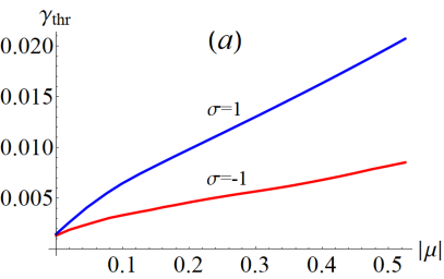
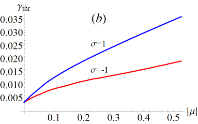
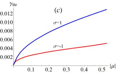
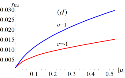
Figure 3: (Colour online.) Threshold current as a function of the impurity strength $\mu$ for $\kappa=1$: $\alpha=0.02$ (a) and $\alpha=0.05$ (b); $\kappa=2$: $\alpha=0.02$ (c) and $\alpha=0.05$ (d). Blue colour corresponds to $\sigma=1$ and red corresponds to $\sigma=-1$.

The difference $|\gamma^{+}_{thr}-\gamma^{-}_{thr}|$ increases as $\kappa$ increases and decreases as $\alpha$ decreases. The only principal difference can be seen in the limit $\mu\to 0$. The threshold current does not vanish and this is a consequence of the discreteness. Even if there is no impurity some non-zero bias is necessary to overcome the PN barrier. In the continuum the threshold current would be exactly zero for $\mu=0$.

Calculation of the fluxon scattering in the limit of very strong discreteness is complicated due to different reasons. Among them there are dynamical chaos, creation of fluxon-antifluxon pairs and the multiplicity of the moving dc-driven fluxons that coexist for the same value of the dc bias. It is well known for the finite size JTLs [30, 31, 32] that the discreteness of the media brings the fundamental change to the velocity-bias $v=v(\gamma)$ dependence, which switches from the monotonous curve in the continuum to the piecewise dependence in the discrete case. Each curve corresponds to the resonance with the particular cavity mode. The hysteresis is clearly seen for the large bias values while for the small bias and, especially for the weak discreteness the $v=v(\gamma)$ it hardly can be observed. In the almost infinite JTLs the cavity modes play no role because they decay over the lattice. However, we have observed how the coexistence of two fluxons with the different essentially non-relativistic velocities can be manifested. In Fig. 4 the change of the fluxon velocity after the scattering is demonstrated for rather small values of discreteness, namely $\kappa=0.55$ and $\kappa=0.6$. The fluxon is launched from the same starting point, therefore both the trajectories coincide before the interaction with the qubit. But they diverge after the interaction.

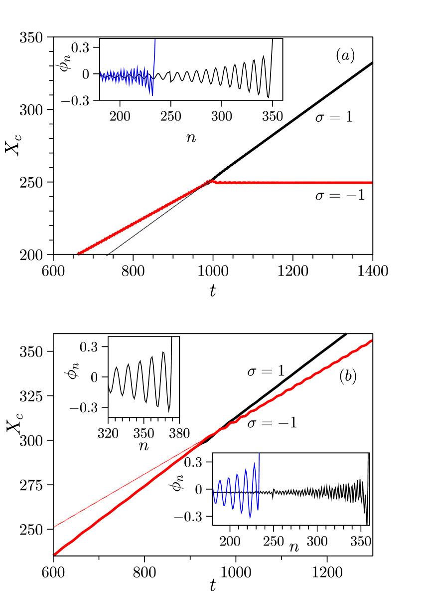
Figure 4: (Colour online.) Fluxon center of mass evolution for $\alpha=0.02$, $\kappa=0.6$, $\gamma=0.0285$ (a) and $\kappa=0.55$, $\gamma=0.037$ (b). Thick black and red lines correspond to the positive and negative qubit polarity, respectively. Thin dotted straight lines satisfy $X_{c}\propto vt$, where $v$ is the fluxon velocity after interaction with the qubit. They are plotted to highlight the fluxon velocity change after the interaction. The insets show the details of the fluxon tail before (blue) and after (black) the interaction. See text for details.

In the case shown in Fig. 4a the fluxon attains higher velocity after passing the qubit with $\sigma=1$. After passing the $\sigma=-1$ qubit the fluxon gets trapped. The lattice size is $N=500$, the integration time is $t\sim 1000\gg 1/\alpha$. So it is quite clear that before and after passing the impurity we are dealing with the different attractors of the system that have different equilibrium velocities. Before hitting the impurity the fluxon had velocity $v\approx 0.15$ and after the interaction it acquired higher velocity $v\approx 0.20$. The thin dashed line $X_{c}\propto 0.2t$ is plotted in order to highlight the velocity change. The oscillating tails behind the fluxon additionally confirm that these are two different fluxon attractors that are coupled to plasmons with different wavelengths (see the respective inset). This is typical situation [33], when the topological solitons, moving with different velocities, excite different plane waves with different wavelengths. These wavelengths satisfy the resonance condition $vq=\omega_{L}(q)$, where $\omega_{L}(q)=[(1-\gamma^{2})^{1/2}+4\kappa\sin^{2}(q/2)]^{1/2}$ is the plasmon dispersion law that can be easily derived from the DSG equation. This equation always has at least one root and if $v$ is small enough it will have multiple roots. A similar situation is illustrated in Fig. 4b. Here the fluxon passes the $\sigma=1$ qubit without any change of velocity. Also, the wavelength of the plasmon tail remains the same, as can be observed after comparing the upper inset (after interaction) and the blue dependence in the lower inset (before interaction). On the other hand, the fluxon loses its velocity after passing the $\sigma=-1$ qubit. Comparison of the oscillating tails behind the fluxon before and after the scattering clearly shows the change in the tail wavelength.

4 Qubit delay time

4.1 Qubit delay time for the infinite JTL.

In the fluxon assisted qubit readout process it is important to maximize the time difference between the fluxon passage time through the $\sigma=-1$ and $\sigma=+1$ impurities. By measuring those times, an experimentalist can determine the qubit state. Thus, we have focused on the computation of the difference

$$\Delta t=|t_{+}-t_{-}|,$$ (21)

which we should call the delay time and where $t_{\pm}$ is the time necessary for the fluxon to travel from one end of the JTL to another one. The subscripts in $t_{\pm}$ correspond to the respective polarity of the impurity, $\mbox{sign}(\sigma)$.

The main results are given in Fig. 5 where the dependence of the delay time is given as a function of the external bias $\gamma$ for the different values of the JTL discreteness parameter $\kappa$.

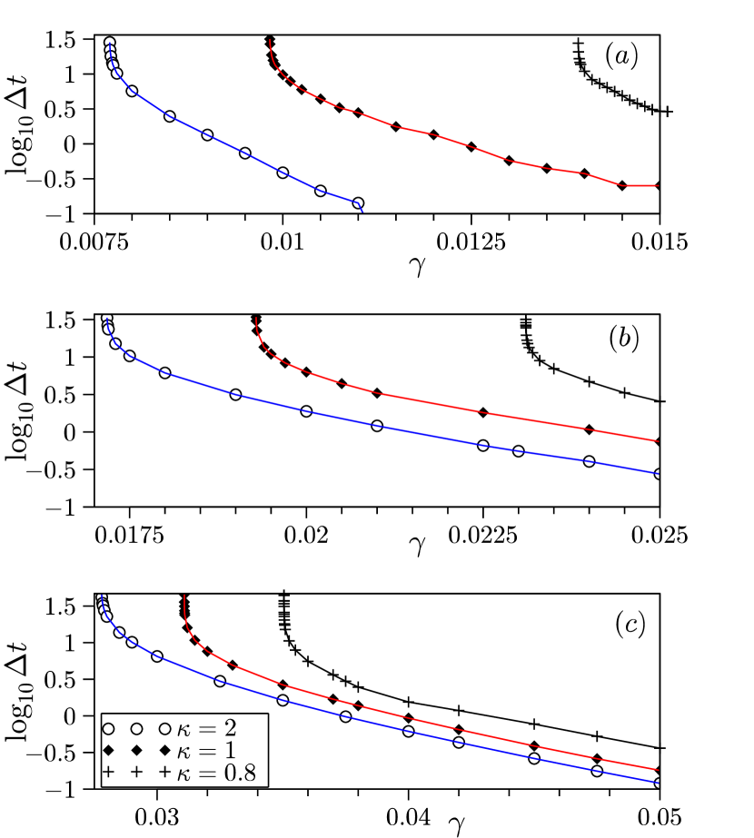
Figure 5: (Colour online.) Decimal logarithm of the delay time on the qubit as a function of the dimensionless bias for the different values of the discreteness parameter and damping [$\alpha=0.02$ (a), $\alpha=0.05$ (b) and $\alpha=0.1$ (c)]. The discreteness values are given in the legend and $|\mu|=0.2$. Solid lines are drawn as a guide for an eye.

One can observe that the delay time increases significantly for the fixed bias value as the JTL becomes more discrete. For example, compare the values of $\Delta t$ for the same values of damping ($\alpha=0.05$) and bias ($\gamma=0.02$). For $\kappa=1$ we have $\Delta t\approx 2.13$ and for $\kappa=2$ we have $\Delta t\approx 6.3$, hence a threefold increase when the coupling constant is decreased by half. The singular behavior of $\Delta t$ at some bias value can be clearly seen. This value equals $\gamma_{thr}^{+}$ at which the fluxon still has enough energy to pass the $\sigma=-1$ qubit, but is trapped by the $\sigma=1$ qubit. Thus, the bias values $\gamma\gtrsim\gamma_{thr}^{+}$ are the most desirable from the point of view of best readout sensitivity.

4.2 Influence of the JTL size on the delay time

In most of the experiments with the JTLs their length is not very big. They are significantly shorter than used in the numerical simulations in the previous sections. Normally the array length is about $N\sim 10\div 30$ junctions [6, 7, 32]. In such short arrays the boundary effects are important. In order to assess them the simulations for the short linear JTL with $N=30$ have been performed. We simulated numerically the situation when the soliton was launched at the site $n=5$ and computed the passage time that elapsed when the fluxon reached the site $n=25$. The delay time $\Delta t$ as a function of the external bias $\gamma$ is given in Fig. 6. Different panels correspond to the different values of damping $\alpha$. One can observe the main features from the almost infinite junction case discussed in the previous subsection. Strongly non-monotonic behaviour appears because the fluxon center of mass has an oscillating component. If dissipation is too small, as in the case of $\alpha=0.02$ (Fig.6a), these oscillations still persist when the fluxon reaches the end of the junction, as shown in the inset to that figure. Thus, if the bias is too strong, the difference between the passage times for the different qubit states is less than the oscillation of the fluxon center. Therefore, no qubit readout is possible. However, for the bias values $\gamma\gtrsim\gamma^{+}_{thr}$ the delay time is well defined similarly to the infinite JTL case described in Subsec. 4.1.

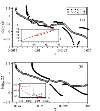
Figure 6: (Colour online.) Decimal logarithm of the delay time for the array with $N=30$ junctions as a function of the bias $\gamma$ for $\kappa=1$ and $\kappa=2$ (see the legend) and $\alpha=0.02$ (a), $\alpha=0.05$ (b). The inset in panel (a) shows the trajectories of the fluxon for interacting with the $\sigma=1$ (black line) and $\sigma=-1$ (red line) impurities. The dc bias equals $\gamma=0.01$. The inset in panel (b) the passage $t_{\pm}$ times are given for the case $\kappa=2$, $\alpha=0.05$. In all figures $|\mu|=0.2$.

The delay time $\Delta t$ for the fixed bias increases as $\kappa$ is decreased. For the larger values of dissipation the dependencies become more regular because the oscillating component of the fluxon center of mass decays faster. The threshold values $\gamma^{\pm}_{thr}$ are approximately the same as in the almost infinite case (see the inset to Fig. 6b).

5 Discussion and conclusions

This article is devoted to the studies of the fluxon interaction with the dipole impurity in the Josephson junction array [Josephson transmission line (JTL)]. The dipole impurity describes the inductively coupled to the JTL qubit. The impurity has two values of polarity $\sigma=\pm 1$ that correspond to different states of the qubit. By scattering a fluxon on the qubit and measuring its passage time, one can distinguish between the different qubit states because the fluxon interacts differently with the $\sigma=-1$ and $\sigma=1$ impurities [13, 14]. Hence, it is important to maximize the difference $\Delta t$ between the abovementioned passage times. In this work we addressed the question how the discreteness of the JTL influences $\Delta t$.

Our findings can be summarized by the diagram shown in Fig. 7.

Figure 7: Schematic representation of the different scenarios of the delay time detection as a function of the external bias. (see text).

Depending on the value of the external dc bias, there are three sectors:

• $0<\gamma<\gamma^{-}_{thr}$. In this sector the bias is too small and fluxon propagation is not possible. Hence, no readout process.

• $\gamma^{-}_{thr}<\gamma<\gamma^{+}_{thr}$. Fluxon is always trapped on the $\sigma=+1$ qubit and, at the same time, passes the $\sigma=-1$ qubit. Thus, the delay time is infinite. In this case it is desirable to increase this bias interval. Our results demonstrate that with the increase of discreteness this interval decreases. At some point ($\kappa\sim 0.5$) the threshold values for different polarities coincide. We did not venture for lower values of $\kappa$. Thus, we conclude that discreteness poses a destructive effect for the fluxon readout in this bias range.

• $\gamma>\gamma^{+}_{thr}$. In this case the fluxon passes throughout the qubits with both polarities. The delay time $\Delta t$ helps us to assess the effectiveness of the readout process. It is desirable to maximize this time. We have observed that the delay time increases significantly if discreteness becomes stronger. In particular, for the fixed bias values, $\Delta t$ can increase by the factor of $2$ or even more if the discreteness constant is halved. If discreteness slows down the fluxon motion it will naturally increase the delay time. Hence, if one applies the dc bias at $\gamma\gtrsim\gamma^{+}_{thr}$ the sensitivity of the readout process is better for the more discrete JTLs.

Also we would like to note that for the essentially discrete JTLs the hysteresis effects on the velocity-bias (or current-voltage characteristics) can be strong. This means that for the fixed bias value several fluxon attractors with different velocities coexist. As a result, a clear definition of the delay time on the qubit is complicated because it depends on the initial conditions. This hysteresis phenomenon is well-documented experimentally and theoretically [30, 31, 32] for the short junction when the cavity modes play an important role. In our work we have encountered yet another manifestation of this hysteresis, but for the almost infinite lines, when the fluxon jumps to an attractor with a different velocity after interacting with the qubit. This scattering can be both accelerating and decelerating, e.g. the fluxon switches to the larger or smaller velocity after the scattering depending on the qubit polarity. We believe that this phenomenon must occur not just for the dipole impurity but for other types of impurities. It requires a more detailed investigation that will be reported elsewhere.

References

- [1] A. Barone, G. Paterno, Physics and Applications of the Josephson Effect, Wiley, New York, 1982.
- [2] K. K. Likharev, Dynamics of Josephson Junctions and Circuits, Gordon and Breach, New York, 1986.
- [3] T. A. Fulton, R. C. Dynes, Single vortex propagation in Josephson tunnel junctions, Solid State Comm. 12 (1973) 57–61.
- [4] A. Davidson, B. Dueholm, B. Kryger, N. Pedersen, Experimental investigation of trapped sine-Gordon solitons, Phys. Rev. Lett. 5 (1985) 2059–2062.
- [5] A. V. Ustinov, Solitons in Josephson junctions, Physica D 123 (1-4) (1998) 315–329.
- [6] E. Trías, J. J. Mazo, T. P. Orlando, Discrete breathers in nonlinear lattices: Experimental detection in a Josephson array, Phys. Rev. Lett. 84 (4) (2000) 741–744.
- [7] P. Binder, D. Abraimov, A. V. Ustinov, S. Flach, Y. Zolotaryuk, Observation of breathers in Josephson ladders, Phys. Rev. Lett. 84 (4) (2000) 745–748.
- [8] E. Ben-Jacob, I. Goldhirsch, Y. Imry, S. Fishman, Intermittent chaos in Josephson junctions, Phys. Rev. Lett. 49 (1982) 1599–1502.
- [9] R. L. Kautz, Noise, chaos, and the Josephson voltage standard, Rep. Prog. Phys. 59 (8) (1996) 935.
- [10] N. Lazarides, G. P. Tsironis, Multistability and self-organization in disordered SQUID metamaterials, Supercond. Sci. Technol. 26 (8) (2013) 084006.
- [11] R. Behr, O. Kieler, J. Kohlmann, F. Müller, L. Palafox, Development and metrological applications of Josephson arrays at ptb, Meas. Sci. Technol. 23 (12) (2012) 124002.
- [12] A. Kemp, A. Wallraff, A. Ustinov, Josephson vortex qubit: Design, preparation and read-out, Phys. Status Solidi (b) 233 (3) (2002) 472–481.
- [13] D. V. Averin, K. Rabenstein, V. K. Semenov, Rapid ballistic readout for flux qubits, Phys. Rev. B 73 (2006) 094504.
- [14] A. Fedorov, A. Shnirman, G. S. A. Kidiyarova-Shevchenko, Reading out the state of a flux qubit by Josephson transmission line solitons, Phys. Rev. B 75 (22) (2007) 224504.
- [15] A. N. Price, A. Kemp, D. R. Gulevich, F. V. Kusmartsev, A. V. Ustinov, Vortex qubit based on an annular Josephson junction containing a microshort, Phys. Rev. B 81 (2010) 014506.
- [16] K. G. Fedorov, A. V. Shcherbakova, R. Schäfer, A. V. Ustinov, Josephson vortex coupled to a flux qubit, Appl. Phys. Lett. 102 (2013) 132602.
- [17] K. G. Fedorov, A. V. Shcherbakova, M. J. Wolf, D. Beckmann, A. V. Ustinov, Fluxon readout of a superconducting qubit, Phys. Rev. Lett. 112 (2014) 160502.
- [18] I. I. Soloviev, N. V. Klenov, A. L. Pankratov, L. S. Revin, E. Il’ichev, L. S. Kuzmin, Soliton scattering as a measurement tool for weak signals, Phys. Rev. B 92 (1) (2015) 014516.
- [19] W. Wustmann, K.D. Osborn, Reversible fluxon logic: Topological particles allow ballistic gates along one-dimensional paths, Phys. Rev. B 101 (1) (2020) 014516.
- [20] K. D. Osborn, W. Wustmann, Asynchronous Reversible Computing Unveiled Using Ballistic Shift Registers, Phys. Rev. Applied 19 (5) (2023) 054034.
- [21] I. O. Starodub, Y. Zolotaryuk, Fluxon interaction with the finite-size dipole impurity, Phys. Lett. A 383 (13) (2019) 1419–1426.
- [22] T. Fraggis, S. Pnevmatikos, E. Economou, Excitation of the impurity mode by topological solitons in a atomic chain, Phys. Lett. A 142 (6) (1989) 361–366.
- [23] O. M. Braun, Y. S. Kivshar, Nonlinear dynamics of the Frenkel-Kontorova model with impurities, Phys. Rev. B 43 (1991) 1060–1073.
- [24] Y. S. Kivshar, B. A. Malomed, Dynamics of solitons in nearly integrable systems, Rev. Mod. Phys. 61 (1989) 763–915.
- [25] S. A. Gredeskul, Y. S. Kivshar, Propagation and Scattering of Nonlinear Waves in Disordered Systems, Phys. Rep. 216 (1992) 1–61.
- [26] L. G. Aslamazov, E. V. Gurovich, Pinning of solitons by abrikosov vortices in distributed Josephson junctions, JETP Lett. 40 (1984) 746–749.
- [27] O. M. Braun, Y. S. Kivshar, The Frenkel-Kontorova Model: Concepts, Methods, and Applications, Springer, Berlin, 2003.
- [28] Y. S. Kivshar, B. A. Malomed, A. A. Nepomnyashchy, Interaction of fluxon with localized inhomogeneity in a long Josephson junction, JETP 94 (1988) 356–365.
- [29] D. W. McLaughlin, A. C. Scott, Perturbation analysis of fluxon dynamics, Phys. Rev. A 18 (4) (1978) 1652.
- [30] A. V. Ustinov, M. Cirillo, B. A. Malomed, Fluxon dynamics in one-dimensional Josephson-junction arrays, Phys. Rev. B 47 (1993) 8357–8360.
- [31] S. Watanabe, H. S. J. van der Zant, S. H. Strogatz, T. E. Orlando Dynamics of circular arrays of Josephson junctions and the discrete sine-Gordon equation, Physica D 97 (1996), 429–470.
- [32] J. Pfeiffer, A. A. Abdumalikov, Jr., M. Schuster, A. V. Ustinov, Resonances between fluxons and plasma waves in underdamped Josephson transmission lines of stripline geometry, Phys. Rev. B 77 (2) (2008), 024511.
- [33] O. Braun, B. Hu, A. Zeltser, Driven kink in the Frenkel-Kontorova model, Phys. Rev. E 62 (3) (2000) 4235–4245.