First-order effect of electron-electron interactions on the anomalous Hall conductivity of massive Dirac fermions

Abstract

We investigate the first-order correction to the anomalous Hall conductivity of 2D massive Dirac fermions arising from electron-electron interactions. In a fully gapped system in the limit of zero temperature, we find that this correction vanishes, confirming the absence of perturbative corrections to the topological Hall conductivity. At finite temperature or chemical potential, we find that the total Hall response decays faster than in the non-interacting case, depending on the strength of electron-electron interactions. These features, which could potentially be observed experimentally, show the importance of two-body interactions for anomalous Hall transport.

Introduction—After the discovery of the quantum Hall effect, theoretical effort was directed towards understanding the robustness of the quantisation of the Hall conductivity $\sigma_{H}$, which in the absence of interactions is related to a topological invariant [3, 4]. In a seminal paper [5], Coleman and Hill showed that two-particle interactions do not modify the value of $\sigma_{H}$ at zero temperature, if the Fermi energy lies in the bulk band gap, which was later generalised to nonrelativistic interactions in Ref. [6]. This raises the question whether the Hall conductivity is robust to the effects of interactions in systems at finite temperature or chemical potential. To answer this question, we investigate the impact of electron-electron (e-e) interactions in the archetypal model of the anomalous Hall effect [7], a two-dimensional system of massive Dirac fermions.

Aside from its foundational significance, this issue also holds practical implications since real-world materials exist at non-zero temperatures and are rarely completely free of doping. It has been demonstrated [8, 9, 10] that certain many-body interactions, for example that between electrons and quenched disorder, can substantially influence Hall responses. For instance, in the anomalous and spin-Hall effects, the presence of quenched disorder can yield outcomes remarkably at odds with non-interacting results  [11, 12]. These include a faster decay of Hall responses with growing chemical potential, changes in sign, and, in some cases, even the complete elimination of these effects. However, while it may be possible to mitigate disorder in a material by refining the growth process, the omnipresent e-e interactions cannot be easily eliminated. Thus, it is fundamental to understand how they affect the Hall response to be able to predict and explain experimental results.

In this paper, we study the correction to the anomalous Hall effect of massive Dirac fermions to first-order in the strength of e-e interactions. We start by introducing the model Hamiltonian and calculate the zeroth- and first-order response functions. We find that the first-order response is divergent. Divergences can be removed by renormalising the bare parameters which enter the model. In this way, we obtain a finite expression for the first-order correction to the Hall conductivity.

The first-order correction naturally depends on the form of the e-e interaction. Here, we initially address the case of a contact potential, whose relative simplicity allows us to do significant analytical progress. We relate such potential to the Coulomb interaction amongst electrons in an overscreened regime. We show that interaction corrections can be large enough to counterbalance the non-interacting contribution to the Hall conductivity. In particular, we show that the anomalous Hall conductivity can decay faster with chemical potential than what is predicted in the non-interacting case. We then compute the same correction for an unscreened Coulomb potential, and show that it exhibits similar features. Thus, we confirm that they are robust irrespective of the precise form of the interaction.

Description of the model—We consider massive Dirac fermions in two dimensions, whose dynamics is described by the many-body Hamiltonian (hereafter, we set $\hbar=1$)

$$\hat{\mathcal{H}}= \sum_{\alpha\beta,\bm{k}}\hat{\psi}^{\dagger}_{\alpha,\bm{k}}\Big{(}\bm{d}(\bm{k})\cdot\bm{\sigma}_{\alpha\beta}-\mu\,\delta_{\alpha\beta}\Big{)}\hat{\psi}_{\beta,\bm{k}}+$$

$$+\frac{1}{2} \sum_{\bm{q}\neq 0}\sum_{\alpha\bm{k},\beta\bm{k}^{\prime}}\hat{\psi}^{\dagger}_{\alpha,\bm{k}-\frac{\bm{q}}{2}}\hat{\psi}^{\dagger}_{\beta,\bm{k}^{\prime}+\frac{\bm{q}}{2}}V_{\bm{q}}\hat{\psi}_{\beta,\bm{k}^{\prime}-\frac{\bm{q}}{2}}\hat{\psi}_{\alpha,\bm{k}+\frac{\bm{q}}{2}},$$ (1)

where $\psi_{\lambda,\bm{k}}$ $(\psi^{\dagger}_{\lambda,\bm{k}})$ destroys (creates) a particle with momentum $\bm{k}$ and pseudospin $\lambda$, $\mu$ is the chemical potential, $H(\bm{k})=\bm{d}(\bm{k})\cdot\bm{\sigma}$ is the single-particle Hamiltonian, $\bm{d}(\bm{k})=(v_{\text{F}}k_{x},v_{\text{F}}k_{y},\Delta)$ and $\bm{\sigma}=(\sigma_{x},\sigma_{y},\sigma_{z})$ is a vector of Pauli matrices. Here, $\Delta$ is half the band gap, while $v_{\text{F}}$ is the Fermi velocity. The energy of these particles is $\pm\varepsilon_{k}$, where $\varepsilon_{k}=\sqrt{(v_{\text{F}}k)^{2}+\Delta^{2}}$ and the $\pm$ sign identifies the conduction and valence bands, respectively. Finally, $V_{\bm{q}}$ is the e-e interaction, which will be specified later. The non-interacting Matsubara Green’s function (MGF) corresponding to our Hamiltonian takes the form $G^{(0)}(\bm{k},i\omega_{n})=\big{[}(i\omega_{n}+\mu)\sigma_{0}-H(\bm{k})\big{]}^{-1}$, where $i\omega_{n}$ is a fermionic Matsubara frequency and $\sigma_{0}$ is the unit matrix.

Within the linear-response formalism [13], the Hall conductivity is defined in terms of the current-current response function $\chi_{j_{x}j_{y}}(\bm{q},\omega)$ as

$$\sigma_{H}=\lim_{\omega\to 0}\left[\frac{ie^{2}}{\omega}\chi_{j_{x}j_{y}}(\bm{q}=0,\omega)\right]\!.$$ (2)

Fig. 1 summarises the diagrammatic calculation of $\chi_{j_{x}j_{y}}(\bm{q},i\omega)$ to zeroth [panel (a)] and first-order [panels (b)–(d)] in the e-e interaction. There, solid lines represent non-interacting MGFs, while dashed lines represent the e-e interaction. Finally, the solid dots are the current operators $j_{x/y}=v_{\text{F}}\sigma_{x/y}$.

Zeroth order contribution— At zeroth order in interaction we find the Hall conductivity [13]

$$\sigma_{H}^{(0)}(\mu,T)=-\frac{e^{2}}{2h}\Big{(}1-\mathcal{F}_{-2}^{+}(\bar{\mu},\bar{T})\Big{)},$$ (3)

which recovers  the well-known zero-temperature result for the anomalous Hall conductivity at a finite doping (see, e.g., Ref. [16]), as well as the finite-temperature generalisation of the Chern number, the so-called “Ulhmann number” [17]. In Eq. (3) we defined the integral

$$\mathcal{F}_{n}^{\pm}=\!\int_{1}^{\infty}\!\!\!dx~{}x^{n}\!\!\left(\frac{1}{e^{(x-\bar{\mu})/\bar{T}}+1}\!\pm\!\frac{1}{e^{(x+\bar{\mu})/\bar{T}}+1}\right)\!\!,$$ (4)

where $\bar{\mu}=\mu/\Delta$, $\bar{T}=k_{\text{B}}T/\Delta$ are the chemical potential and the temperature, measured in units of (half) the gap.

Figure 1: Panel (a) Non-interacting contribution to the current-current response function $\chi_{j_{x}j_{y}}(\bm{q},i\omega)$. Panels (b)–(d) are the first-order contributions to $\chi_{j_{x}j_{y}}(\bm{q},i\omega)$ due to vertex corrections [panel (b)], and self-energy insertions [panels (c) and (d)]. In these diagrams, solid lines are MGFs, dashed lines represent electron-electron interactions, while solid dots stand for current vertices.

First order contribution—Fig. 1 (b) and (c)–(d) show the first-order diagrams which yield the exchange and self-energy corrections to $\sigma_{H}$, respectively .

We start by evaluating the self-energy insertion, i.e.

$$\Sigma(\bm{k})=\leavevmode\hbox to0pt{\vbox to0pt{\text{[drawing]}}}=\Sigma_{0}(\bm{k})\sigma_{0}+\bm{\Sigma}(\bm{k})\cdot\bm{\sigma}, \mathbf{k}^{\prime},i\omega_{n}^{\prime} V(\mathbf{k}-\mathbf{k}^{\prime}) \mathbf{k}^{\prime},i\omega_{n}^{\prime} V(\mathbf{k}-\mathbf{k}^{\prime})$$ (5)

where

$$\Sigma_{0}(\bm{k})\, =\frac{1}{2}\int\frac{d^{2}{\bm{k}^{\prime}}}{(2\pi)^{2}}\,V(\bm{k}-\bm{k}^{\prime})\Phi^{+}_{k^{\prime}},$$ (6)

$$\bm{\Sigma}(\bm{k})\, =-\frac{1}{2}\int\frac{d^{2}{\bm{k}^{\prime}}}{(2\pi)^{2}}\,\frac{\bm{d}(\bm{k}^{\prime})}{\varepsilon_{k^{\prime}}}V(\bm{k}-\bm{k}^{\prime})\Phi^{-}_{k^{\prime}},$$ (7)

are independent of the external frequency. We defined $\Phi^{\pm}_{k}=1-f_{h}(\varepsilon_{k})\pm f_{e}(\varepsilon_{k})$, where $f_{e}(\varepsilon)\!=\![e^{(\varepsilon-\mu)/(k_{\text{B}}T)}\!+\!1]^{-1}$ and $f_{h}(\varepsilon)\!=\![e^{(\varepsilon+\mu)/(k_{\text{B}}T)}\!+\!1]^{-1}$ are the Fermi–Dirac distribution functions for electrons and holes, respectively.

Adding the contributions from diagrams 1(b)–(d), and expanding to first-order in frequency, we find the first-order correction to the current-current response function

$$\chi_{j_{x}j_{y}}^{(1)}(\bm{q}=0,i\omega)\to-\frac{\omega v_{\text{F}}^{2}\Delta}{4}\times$$

$$\times\int\frac{d^{2}{\bm{k}}}{(2\pi)^{2}}\,\Bigg{\{}\Bigg{[}\frac{2\Sigma_{0}(\bm{k})}{\varepsilon_{k}^{3}}\frac{\partial\Phi^{+}_{k}}{\partial\varepsilon_{k}}\Bigg{]}-\Bigg{[}\frac{2\Sigma_{\perp}(\bm{k})}{\varepsilon_{k}^{2}\Delta}\frac{\partial\Phi^{-}_{k}}{\partial\varepsilon_{k}}\Bigg{]}+$$

$$+\int\frac{d^{2}{\bm{k}^{\prime}}}{(2\pi)^{2}}\,V(\bm{k}-\bm{k}^{\prime})\frac{v_{\text{F}}^{2}(\bm{k}\cdot\bm{k}^{\prime}-k^{\prime 2})}{\varepsilon_{k}^{3}\varepsilon_{k^{\prime}}^{2}}\frac{\partial\Phi^{-}_{k^{\prime}}}{\partial\varepsilon_{k^{\prime}}}\Phi^{-}_{k}\Bigg{\}},$$ (8)

where we split $\bm{\Sigma}$ into $\bm{\Sigma}_{\parallel}=(\Sigma_{x},\Sigma_{y})$ and $\Sigma_{\perp}=\Sigma_{z}$. In [14] we show that the terms in the self-energy containing $\bm{\Sigma}_{\parallel}$ cancel exactly similar terms from the exchange diagram. This is a consequence of the Ward identity [19].

Although the contribution from $\bm{\Sigma}_{\parallel}$ cancels between diagrams, Eq. (First-order effect of electron-electron interactions on the anomalous Hall conductivity of massive Dirac fermions) still depends on $\Sigma_{0}(\bm{k})$ and $\Sigma_{\perp}(\bm{k})$, both of which suffer from ultraviolet (UV) divergences and must be regularized by introducing a cutoff $\Lambda$ (see below). For a contact potential $V({\bm{k}})=V_{c}$, where $V_{c}$ is a constant which does not depend on the momentum carried by the interaction, these divergences are quadratic $\propto\Lambda^{2}$ (for $\Sigma_{0}$) or linear $\propto\Lambda$ (for $\bm{\Sigma}_{\parallel}$ and $\Sigma_{\perp}$). For a Coulomb potential $V({\bm{k}})=2\pi e^{2}/(\kappa k)$ for a medium with dielectric constant $\kappa$, the quadratic divergence becomes linear, while the linear ones become logarithmic.

Regularization of divergences—In order to deal with these divergences, we introduce the UV cutoff in momentum $\Lambda$ by employing a type of Pauli–Villars [19] regularisation scheme: the interaction is modified in such a way as to vanish fast enough at large momentum, so that the integrals become convergent. More explicitly, the interaction becomes $V(\bm{k})\to V(\bm{k})\big{[}1+(|\bm{k}|/\Lambda)^{n}\big{]}^{-1}$, where $n$ is a natural number. The integrals in Eq. (First-order effect of electron-electron interactions on the anomalous Hall conductivity of massive Dirac fermions) then contain cutoff-dependent pieces signifying the presence of divergences, as well as finite parts. The latter become independent of the cutoff in the limit $\Lambda\to\infty$.

UV divergences are absorbed into the redefinition of the parameters which enter into the Hamiltonian. Bare parameters ($x^{\text{bare}}$, where $x\equiv\mu,v_{\text{F}},\Delta$) are defined in terms of physical ones ($x^{\text{ph}}$) as $x^{\text{bare}}=x^{\text{ph}}+\delta x^{\text{CT}}$. Here, $\delta x^{\text{CT}}$ are the counterterms. From here on, we assume the Hamiltonian is defined in terms of renormalised parameters and hence omit the label “ph”.

Using the Dyson equation and the expression given in Eq. (5), we write the dressed MGF as a function of the bare parameters

$$G^{-1}(\bm{k}) = \left(i\omega_{n}+\mu+\delta\mu^{\text{CT}}-\Sigma_{0}(\bm{k})\right)\sigma_{0}$$ (9)

$$- \left(\bm{d}(\bm{k})+\delta\bm{d}^{\text{CT}}(\bm{k})+\bm{\Sigma}(\bm{k})\right)\cdot\bm{\sigma},$$

where $\delta\bm{d}^{\text{CT}}(\bm{k})=(\delta v_{\text{F}}^{\text{CT}}k_{x},\delta v_{\text{F}}^{\text{CT}}k_{y},\delta\Delta^{\text{CT}})$. The divergences introduced by $\Sigma_{0}(\bm{k})$, $\bm{\Sigma}_{\parallel}(\bm{k})$ and $\Sigma_{\perp}(\bm{k})$ are cancelled by the renormalisation of the chemical potential, Fermi velocity and energy gap, respectively. The details of this renormalisation can be found in [14], and they are consistent with previous results from Refs. [21, 22].

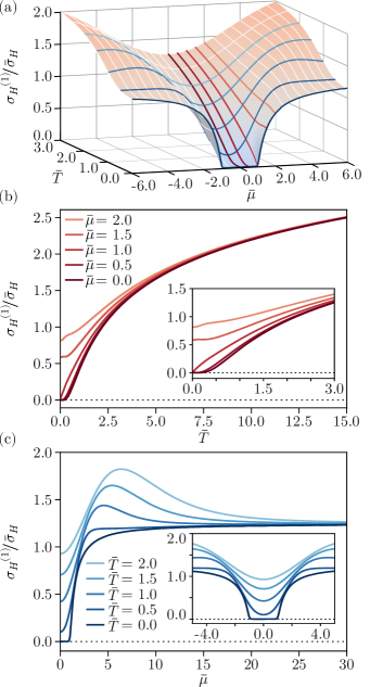
Figure 2: Panel (a) The first-order correction due to contact e-e interactions to the Hall conductivity, $\sigma_{H}^{(1)}$, as a function of both chemical potential and temperature in units of $\bar{\sigma}_{H}=(N_{0}V_{c})e^{2}/(2h)$. Panel (b) The correction $\sigma_{H}^{(1)}$ as a function of temperature, for various chemical potentials, along the cuts shown in the same colors in (a). A logarithmic divergence at high temperatures can be observed. Panel (c) The correction $\sigma_{H}^{(1)}$ as a function of the chemical potential, along the cuts shown in the same colors in (a), for fixed values of the temperature. At large doping, curves converge to the finite value of $5/4$. Insets: magnifications of the main plots in a similar range of values as the 3D plot.

We remark a notable feature of the Hall response. As shown above, the renormalisation of the Fermi velocity is needed for the propagator in (9) to be finite. However, due to the topological nature of the Hall response, i.e. the fact that $\chi_{j_{x}j_{y}}^{(0)}$ is independent of $v_{\text{F}}$, no additional first-order counterterm diagram is produced from $\chi_{j_{x}j_{y}}^{(0)}$ as a consequence of the renormalisation $v_{\text{F}}\to v_{\text{F}}+\delta v_{\text{F}}^{\text{CT}}$. Thus, we can let $v_{\text{F}}\to v_{\text{F}}^{\text{ph}}$ everywhere. This in turn implies that the renormalisation of the chemical potential and band gap are sufficient to ensure the finiteness of first-order diagrams. This is precisely the cancellation of the $\bm{\Sigma}_{\parallel}$ terms between self-energy and vertex diagrams.

After some lengthy algebra [14], we find that the contribution from the first-order diagrams for the case of contact interaction is

$$\sigma_{H}^{(1)}=\frac{\bar{\sigma}_{H}}{2}\Big{[}\mathcal{F}_{-2}^{+}\Big{(}1\!-\!\mathcal{F}_{-2}^{+}\!-\!2\mathcal{F}_{0}^{+}\Big{)}\!-\!2\mathcal{F}_{1}^{-}\mathcal{F}_{-3}^{-}\!+$$

$$+\mathcal{F}_{0}^{+}\Big{(}f_{h}(\Delta)\!+\!f_{e}(\Delta)\!+\!1\Big{)}\!-\!\mathcal{F}_{1}^{-}\Big{(}f_{h}(\Delta)\!-\!f_{e}(\Delta)\Big{)}\Big{]}.$$ (10)

This equation is the central result of our paper. We re-introduced the factors of $\hbar$ and defined $\bar{\sigma}_{H}=N_{0}V_{c}~{}e^{2}/2h$ as our effective coupling constant multiplied by one fourth of the conductance quantum (since we neglect spin and valley degeneracies). $N_{0}=\Delta/(2\pi\hbar^{2}v_{\text{F}}^{2})$ is the density of states (at zero temperature) at the bottom of the conduction band, $V_{c}$ the contact potential, and the functions $\mathcal{F}_{n}^{\pm}$ are given in Eq. (4).

We evaluate Eq. (First-order effect of electron-electron interactions on the anomalous Hall conductivity of massive Dirac fermions) numerically as a function of both chemical potential and temperature. We start by discussing the case when the factor $N_{0}V_{c}$ is constant, i.e. it is independent of temperature and chemical potential. In this case, the behaviour of the first-order correction to the Hall conductivity as a function of doping and temperature is shown in Fig. 2. The particle-hole symmetry is clearly reflected in the fact that the correction is an even function of the chemical potential.

An important feature of the Hall response that can be inferred from Fig. 2(a) is the fact that the first-order correction vanishes at $\bar{T}=0$ when the chemical potential is placed inside the gap, i.e. $|\bar{\mu}|\leq 1$. This is not by chance, but it is a consequence of the Coleman–Hill theorem [5], which states that there are no perturbative corrections to the topological part of the Hall conductivity. It is worth noting that the validity of this theorem for our model is not a trivial statement, since it was proved to apply to gauge-invariant interactions, and non-retarded e-e interactions break Lorentz invariance . The theorem was extended to non-retarded interactions between electrons described by tight-binding models in Ref. [6].

Fig. 2(b) shows the temperature dependence of the correction $\sigma_{H}^{(1)}$ for a set of values of the chemical potential. All curves have the same asymptotic behaviour, which highlights the logarithmic divergence at high temperatures, i.e. $\sigma_{H}\to\ln 2(\ln\bar{T}+\mathcal{C})\bar{\sigma}_{H}$, where $\mathcal{C}\approx 0.98$.

Fig. 2(c) shows $\sigma_{H}^{(1)}$ as a function of chemical potential for fixed values of temperature. The curve at $\bar{T}=0$ clearly proves the validity of the Coleman–Hill theorem, i.e. the vanishing of the correction to the Hall conductivity within the band gap. In the Fermi liquid regime (i.e. for small temperatures and $|\bar{\mu}|>1$) the correction approaches the limit $\sigma_{H}\to(5\bar{\mu}^{2}-2|\bar{\mu}|-3)/(4\bar{\mu}^{2})\bar{\sigma}_{H}$.

Overscreened Coulomb interactions— When the density of states is large, the interaction is heavily screened. For a static Thomas–Fermi screening [24], the contact potential becomes $V_{c}\approx\nu^{-1}$, where $\nu(\mu,T)=\partial_{\mu}n(\mu,T)$ is the thermodynamical density of states. The effective coupling constant $N_{0}V_{c}$ becomes

$$N_{0}V_{c}=4\bar{T}\left[\int_{|x|>1}dx|x|\cosh^{-2}\left(\frac{x-\bar{\mu}}{2\bar{T}}\right)\right]^{-1}.$$ (11)

The Hall conductivity to first order in interaction, $\sigma_{H}=\sigma_{H}^{(0)}+\sigma_{H}^{(1)}$, is shown with solid lines in Figs. 3(a)–(b). Comparing it with the non-interacting result (dashed lines), we see that e-e interactions in the Fermi liquid regime can be strong enough to offset the non-interacting Hall response: $\sigma_{H}$ vanishes quicker than $\sigma_{H}^{(0)}$ with increasing chemical potential or temperature. This effect is similar to that of white-noise disorder, which is likewise strongly suppressed at high electron concentrations [11].

Fig. 3(b) also shows that the conductivity can become negative at large enough chemical potentials. This feature is most likely an artifact of the truncation to first-order in perturbation theory, since the choice $V_{c}\approx\nu^{-1}$ does not allow the potential to be arbitrarily small. We thus expect that summing higher order terms would remedy this feature.

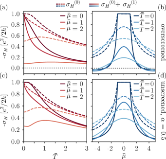
Figure 3: A comparison between the non-interacting ($\sigma_{H}^{(0)}$, dashed lines) and full ($\sigma_{H}=\sigma_{H}^{(0)}+\sigma_{H}^{(1)}$, solid lines) Hall conductivities. Note that an overall minus sign was introduced. Panel (a) Curves are shown as a function of temperature for fixed values of the chemical potential when the Coulomb interaction is heavily screened. Panel (b) Same as Panel (a), but as a function of chemical potential and for fixed values of temperature. Panels (c) and (d) Curves corresponding to (a) and (b), for an unscreened interaction with $\alpha=0.5$.

Note that even though Eq. (11) is formally valid only when the carrier density is large, we still plotted the dark blue solid line ($\bar{T}=0$) for $|\bar{\mu}|\leq 1$ in Fig. 3(b) for consistency with the other curves. This is because, thanks to the Coleman–Hill theorem, $\sigma_{H}^{(1)}$ is always zero in that region, irrespective of the exact form of $V_{c}$. A similar reasoning holds for the dark red solid line ($\bar{\mu}=0$) in Fig. 3(a) at very low temperatures.

Unscreened Coulomb interaction—As before, UV divergences are isolated and absorbed into their corresponding counterterms. The Hall conductivity as a function of temperature and chemical potential is shown in Figs. 3(c) and (d), respectively. The exact expression for $\sigma_{H}$ can be found in [14]. In order to compare these results and those obtained for the Fermi liquid regime, we have chosen the value of the effective fine structure constant $\alpha=e^{2}/(\kappa\hbar v_{\text{F}})=0.5$. Similar to Figs. 3(a)–(b), $\sigma_{H}$ (solid lines) decays faster than $\sigma_{H}^{(0)}$ (dashed lines) as the temperature and the chemical potential increase [panels (c)–(d)]. Since the unscreened Coulomb correction scales linearly with the strength of the e-e interactions, choosing $\alpha=0.5$ gives a weaker effect than the overscreened interaction. Also, note that $\sigma_{H}$ does not become negative in the depicted range of chemical potentials.

In [14] we show that choosing $\alpha=0.8$ instead gives a result of striking similarity with the Fermi liquid regime. For $|\bar{\mu}|\gtrsim 3$, the Hall conductivity becomes negative, thus exhibiting the same artifact as Fig. 3(b).

Conclusion—We calculated the first-order correction to the Hall conductivity due to e-e interactions. Firstly, we showed that the topological part of the Hall conductivity is robust against interactions, in agreement with the Coleman–Hill theorem. Secondly, we found that the effect of interactions can be strong enough to offset the non-interacting contribution. As a result, the total Hall conductivity goes to zero faster than the non-interacting one when either the temperature or the chemical potential increase. These features are present for both heavily screened and unscreened e-e interactions.

A possible experimental platform where these results can be tested is graphene, in a setup in which a gap is opened via substrate effects [25], while the breaking of time-reversal symmetry is realised via proximity induced ferromagnetism [26]. Alternatively, the effect could be observed in transition-metal dichalcogenides where valleys are selectively populated exploiting circular dichroism [27]. We stress that our results are applicable to other effects beyond anomalous Hall transport. We expect similar corrections to exist in, e.g., spin-Hall [28, 29] or orbital-Hall [30, 31] conductivities of sufficiently clean materials, though more work is needed to clarify the impact of e-e interactions on these effects.

Supplemental Materials: First-order effect of electron-electron interactions on the anomalous Hall conductivity of massive Dirac fermions

S1 Zeroth order diagram

In the reverse order of the arrows in the diagram from Fig. 1(a), we use the finite temperature Feynman rules given in Section 6.4 in Ref. [13][Also see the errata for this book, which corrects a minus sign in Rule (vii)] to calculate the non-interacting current-current response function

$$\chi_{j_{x}j_{y}}^{(0)}(\bm{q},i\omega) = \frac{1}{\beta}\sum_{i\omega_{n}}\int_{\bm{k}}\operatorname{Tr}\left[j_{x}G^{(0)}(\bm{k}+\bm{q},i\omega_{n}+i\omega)j_{y}G^{(0)}(\bm{k},i\omega_{n})\right]=-\omega\frac{v_{\text{F}}^{2}\Delta}{2}\int_{\bm{k}}\frac{f_{e}(-\varepsilon_{k})-f_{e}(\varepsilon_{k})}{\varepsilon_{k}^{3}}.$$ (S1)

In this equation we used the shorthand notation $\int_{\bm{k}}=\int d\bm{k}/(2\pi)^{2}$ for the integral, and $\sum_{i\omega_{m}}$ for the sum over Matsubara frequencies. The key advantage for evaluating this sum lies in the fact that the Fermi–Dirac distribution function $f_{e}(z)=[e^{\beta z}+1]^{-1}$ has its poles at fermionic Matsubara frequencies $i\omega_{m}=i(2m+1)\pi/\beta$, where $m$ is an integer, and the corresponding residues are $\mathrm{Res}[f_{e}(z)]=-1/\beta$. For a function of known simple poles, $g(z)=\Pi_{j}(z-z_{j})^{-1}$

$$\mathcal{S}=\frac{1}{\beta}\sum_{i\omega_{m}}g(i\omega_{m})=\sum_{j}\mathop{\mathrm{Res}}_{\,\,z=z_{j}}\big{[}g(z)\big{]}f_{e}(z_{j}).$$ (S2)

After performing a Wick rotation to real frequencies $i\omega\to\omega+i0^{+}$ and using the Kubo formula given in Eq. (2), we obtain the Hall conductivity

$$\sigma_{H}^{(0)}(\mu,T) = -\frac{e^{2}\Delta}{4\pi}\int_{\Delta}^{\infty}d\varepsilon_{k}\frac{f_{e}(-\varepsilon_{k})-f_{e}(\varepsilon_{k})}{\varepsilon_{k}^{2}}~{}.$$ (S3)

Using the Fermi–Dirac-like integral defined before in Eq. (4) and re-introducing the factors of $\hbar$, we finally get

$$\sigma_{H}^{(0)}(\bar{\mu},\bar{T}) = -\frac{e^{2}}{2h}\left(1-\mathcal{F}_{-2}^{+}(\bar{\mu},\bar{T})\right)~{}.$$ (S4)

At zero temperature, we can take the limit of the functions $\mathcal{F}_{n}^{\pm}$

$$\mathcal{F}_{n}^{+}(\bar{\mu},0) = \int_{1}^{|\bar{\mu}|}dx\,x^{n}=~{}\frac{|\bar{\mu}|^{n+1}-1}{n+1}~{},$$ (S5)

$$\mathcal{F}_{n}^{-}(\bar{\mu},0) = \text{sign}(\bar{\mu})\int_{1}^{|\bar{\mu}|}dx\,x^{n}=\text{sign}(\bar{\mu})\frac{|\bar{\mu}|^{n+1}-1}{n+1}~{},$$ (S6)

which are true for $|\bar{\mu}|>1$, but $\mathcal{F}_{n}^{\pm}(|\bar{\mu}|\leq 1,0)=0$ when the chemical potential lies inside the gap.

It can easily be seen that in this limit we get $\sigma_{H}^{(0)}=-e^{2}/2h$ when $|\bar{\mu}|\leq 1$ and $\sigma_{H}^{(0)}(\bar{\mu},0)=-1/|\bar{\mu}|(e^{2}/2h)$ otherwise. This recovers the well-known result for the anomalous Hall conductivity from Ref. [16].

S2 First order diagrams

Using the same Feynman rules for the other 3 diagrams in Fig. 1, we calculate the response functions

$$\!\!\!\!\chi_{j_{x}j_{y}}^{\text{EX}}(0,i\omega) = -\frac{1}{\beta^{2}}\!\!\sum_{i\omega_{n},i\omega_{n}^{\prime}}\!\!\int_{\bm{k},\bm{k}^{\prime}}\!\!\!\!V(\bm{k}-\bm{k}^{\prime})\operatorname{Tr}\left[j_{x}G^{(0)}(\bm{k},i\omega_{n}+i\omega)G^{(0)}(\bm{k}^{\prime},i\omega_{n}^{\prime}+i\omega)j_{y}G^{(0)}(\bm{k}^{\prime},i\omega_{n}^{\prime})G^{(0)}(\bm{k},i\omega_{n})\right]\!,$$ (S7)

$$\!\!\!\!\chi_{j_{x}j_{y}}^{\text{SE}1}(0,i\omega) = -\frac{1}{\beta}\sum_{i\omega_{n}}\int_{\bm{k}}\operatorname{Tr}\left[j_{x}G^{(0)}(\bm{k},i\omega_{n}+i\omega)\Sigma(\bm{k})G^{(0)}(\bm{k},i\omega_{n}+i\omega)j_{y}G^{(0)}(\bm{k},i\omega_{n})\right]\!,$$ (S8)

$$\!\!\!\!\chi_{j_{x}j_{y}}^{\text{SE}2}(0,i\omega) = -\frac{1}{\beta}\sum_{i\omega_{n}}\int_{\bm{k}}\operatorname{Tr}\left[j_{x}G^{(0)}(\bm{k},i\omega_{n}+i\omega)j_{y}G^{(0)}(\bm{k},i\omega_{n})\Sigma(\bm{k})G^{(0)}(\bm{k},i\omega_{n})\right]\!.$$ (S9)

The first one is the easiest to evaluate, and it can be simplified by using a parity transformation $\bm{k}\to-\bm{k}$ and $\bm{k}^{\prime}\to-\bm{k}^{\prime}$. The latter two, however, have second order poles which need to be treated carefully. These poles give rise to derivatives of the occupation functions, and change Eq. (S2) into

$$\mathcal{S}=\frac{1}{\beta}\sum_{i\omega_{m}}g(i\omega_{m})=\!\!\!\!\sum_{j\in\{j_{1},j_{2}\}}\!\!\!\mathop{\mathrm{Res}}_{\,\,z=z_{j}}\big{[}g(z)\big{]}f_{e}(z_{j})+\sum_{j_{2}}\Bigg{[}\frac{df_{e}(z)}{dz}\Big{(}(z-z_{j_{2}})^{2}g(z)\Big{)}\Bigg{]}_{z=z_{j_{2}}}~{},$$ (S10)

where $j_{1}$ and $j_{2}$ are the simple and double poles, respectively.

After summing over the Matsubara frequencies and performing the traces over the Pauli matrices, we find that the first-order current-current response functions are

$$\chi_{j_{x}j_{y}}^{\text{EX}}(0,i\omega)=-\omega\frac{v_{\text{F}}^{2}\Delta}{4}\int_{\bm{k}}\int_{\bm{k}^{\prime}}V(\bm{k}-\bm{k}^{\prime})\Bigg{[}\frac{\varepsilon_{k^{\prime}}^{2}+\Delta^{2}}{\varepsilon_{k^{\prime}}^{3}\varepsilon_{k}^{3}}+\frac{v_{\text{F}}^{2}\bm{k}^{\prime}\cdot\bm{k}}{\varepsilon_{k^{\prime}}^{3}\varepsilon_{k}^{3}}\Bigg{]}\Phi^{-}_{k^{\prime}}\Phi^{-}_{k},$$ (S11)

$$\chi_{j_{x}j_{y}}^{\text{SE}}(0,i\omega)=-\omega\frac{v_{\text{F}}\Delta}{2}\int_{\bm{k}}\Sigma_{0}(\bm{k})\Bigg{[}\frac{v_{\text{F}}}{\varepsilon_{k}^{3}}\frac{\partial\Phi^{+}_{k}}{\partial\varepsilon_{k}}\Bigg{]}+\bm{\Sigma}_{\parallel}(\bm{k})\cdot\frac{v_{\text{F}}^{2}\bm{k}}{\varepsilon_{k}}\Bigg{[}\frac{3}{\varepsilon_{k}^{4}}\Phi^{-}_{k}-\frac{1}{\varepsilon_{k}^{3}}\frac{\partial\Phi^{-}_{k}}{\partial\varepsilon_{k}}\Bigg{]}+\Sigma_{\perp}(\bm{k})\frac{v_{\text{F}}}{\Delta}\Bigg{[}\frac{3\Delta^{2}-\varepsilon_{k}^{2}}{\varepsilon_{k}^{5}}\Phi^{-}_{k}-\frac{\Delta^{2}}{\varepsilon_{k}^{4}}\frac{\partial\Phi^{-}_{k}}{\partial\varepsilon_{k}}\Bigg{]}$$

$$=-\omega\frac{v_{\text{F}}\Delta}{2}\int_{\bm{k}}\Sigma_{0}(\bm{k})\Bigg{[}\frac{v_{\text{F}}}{\varepsilon_{k}^{3}}\frac{\partial\Phi^{+}_{k}}{\partial\varepsilon_{k}}\Bigg{]}-\bm{\Sigma}_{\parallel}(\bm{k})\cdot\frac{v_{\text{F}}^{2}\bm{k}}{\varepsilon_{k}}\frac{\partial}{\partial\varepsilon_{k}}\left(\frac{\Phi^{-}_{k}}{\varepsilon_{k}^{3}}\right)+\Sigma_{\perp}(\bm{k})\frac{v_{\text{F}}}{\Delta}\Bigg{[}\left(\frac{2}{\varepsilon_{k}^{3}}-\frac{3}{\varepsilon_{k}^{4}}\frac{v_{\text{F}}^{2}k^{2}}{\varepsilon_{k}}\right)\Phi^{-}_{k}+\left(\frac{v_{\text{F}}^{2}k^{2}}{\varepsilon_{k}^{4}}-\frac{1}{\varepsilon_{k}^{2}}\right)\frac{\partial\Phi^{-}_{k}}{\partial\varepsilon_{k}}\Bigg{]}$$

$$=-\omega\frac{v_{\text{F}}\Delta}{2}\int_{\bm{k}}\Sigma_{0}(\bm{k})\Bigg{[}\frac{v_{\text{F}}}{\varepsilon_{k}^{3}}\frac{\partial\Phi^{+}_{k}}{\partial\varepsilon_{k}}\Bigg{]}-\bm{\Sigma}_{\parallel}(\bm{k})\cdot\Bigg{[}\bm{\nabla}_{\bm{k}}^{\text{2D}}\left(\frac{\Phi^{-}_{k}}{\varepsilon_{k}^{3}}\right)\Bigg{]}+\Sigma_{\perp}(\bm{k})\Bigg{[}\frac{v_{\text{F}}}{\Delta}\bm{\nabla}_{\bm{k}}^{\text{2D}}\cdot\left(\bm{k}\frac{\Phi^{-}_{k}}{\varepsilon_{k}^{3}}\right)-\frac{v_{\text{F}}}{\varepsilon_{k}^{2}\Delta}\frac{\partial\Phi^{-}_{k}}{\partial\varepsilon_{k}}\Bigg{]},$$ (S12)

where $\Sigma_{0}$ is given in Eq. (6) and we split $\bm{\Sigma}$ from Eq. (7) into $\bm{\Sigma}_{\parallel}=(\Sigma_{x},\Sigma_{y})$ and $\Sigma_{\perp}=\Sigma_{z}$. When integrating the above by parts, $\bm{\nabla}_{\bm{k}}^{\text{2D}}$ gives both vanishing boundary terms and the 2D divergence/gradient of $\bm{\Sigma}_{\parallel}/\Sigma_{\perp}$

$$\bm{\nabla}_{\bm{k}}^{\text{2D}}\cdot\bm{\Sigma}_{\parallel}(\bm{k}) = \bm{\nabla}_{\bm{k}}^{\text{2D}}\cdot\left(-\frac{1}{2}\int_{\bm{k}^{\prime}}\frac{\bm{d}_{\parallel}(\bm{k}^{\prime})}{\varepsilon_{k^{\prime}}}V(\bm{k}-\bm{k}^{\prime})\Phi_{k^{\prime}}^{-}\right)$$ (S13)

$$= -\frac{1}{2}\int_{\bm{k}^{\prime}}\left[\bm{\nabla}_{\bm{k}^{\prime}}^{\text{2D}}\cdot\left(\frac{\bm{d}_{\parallel}(\bm{k}^{\prime})}{\varepsilon_{k^{\prime}}}\right)\Phi_{k^{\prime}}^{-}+\frac{\bm{d}_{\parallel}(\bm{k}^{\prime})}{\varepsilon_{k^{\prime}}}\cdot\bm{\nabla}_{\bm{k}^{\prime}}^{\text{2D}}\left(\Phi_{k^{\prime}}^{-}\right)\right]V(\bm{k}-\bm{k}^{\prime})$$

$$= -\frac{v_{\text{F}}}{2}\int_{\bm{k}^{\prime}}\left[\left(\frac{\varepsilon_{k^{\prime}}^{2}+\Delta^{2}}{\varepsilon_{k^{\prime}}^{3}}\right)\Phi_{k^{\prime}}^{-}+\frac{\bm{k}^{\prime}}{\varepsilon_{k^{\prime}}}\cdot\bm{\nabla}_{\bm{k}^{\prime}}^{\text{2D}}\left(\Phi_{k^{\prime}}^{-}\right)\right]V(\bm{k}-\bm{k}^{\prime}),$$

$$\bm{\nabla}_{\bm{k}}^{\text{2D}}\Sigma_{\perp}(\bm{k}) = \bm{\nabla}_{\bm{k}}^{\text{2D}}\left(-\frac{1}{2}\int_{\bm{k}^{\prime}}\frac{\Delta}{\varepsilon_{k^{\prime}}}V(\bm{k}-\bm{k}^{\prime})\Phi_{k^{\prime}}^{-}\right)$$ (S14)

$$= -\frac{\Delta}{2}\int_{\bm{k}^{\prime}}\left[\bm{\nabla}_{\bm{k}^{\prime}}^{\text{2D}}\left(\frac{1}{\varepsilon_{k^{\prime}}}\right)\Phi_{k^{\prime}}^{-}+\frac{1}{\varepsilon_{k^{\prime}}}\bm{\nabla}_{\bm{k}^{\prime}}^{\text{2D}}\left(\Phi_{k^{\prime}}^{-}\right)\right]V(\bm{k}-\bm{k}^{\prime})$$

$$= -\frac{\Delta}{2}\int_{\bm{k}^{\prime}}\left[\left(-\frac{v_{\text{F}}^{2}\bm{k}^{\prime}}{\varepsilon_{k^{\prime}}^{3}}\right)\Phi_{k^{\prime}}^{-}+\frac{1}{\varepsilon_{k^{\prime}}}\bm{\nabla}_{\bm{k}^{\prime}}^{\text{2D}}\left(\Phi_{k^{\prime}}^{-}\right)\right]V(\bm{k}-\bm{k}^{\prime}).$$

Plugging these expressions back into Eq. (S2) gives an exact cancellation with the exchange response function

$$\chi_{j_{x}j_{y}}^{\text{SE}}(0,i\omega) = -\omega\frac{v_{\text{F}}\Delta}{2}\int_{\bm{k}}\Sigma_{0}(\bm{k})\Bigg{[}\frac{v_{\text{F}}}{\varepsilon_{k}^{3}}\frac{\partial\Phi^{+}_{k}}{\partial\varepsilon_{k}}\Bigg{]}+\bm{\nabla}_{\bm{k}}^{\text{2D}}\cdot\bm{\Sigma}_{\parallel}(\bm{k})\left(\frac{\Phi^{-}_{k}}{\varepsilon_{k}^{3}}\right)-\bm{\nabla}_{\bm{k}}^{\text{2D}}\Sigma_{\perp}(\bm{k})\cdot\left(\frac{v_{\text{F}}\bm{k}}{\Delta}\frac{\Phi^{-}_{k}}{\varepsilon_{k}^{3}}\right)-\Sigma_{\perp}(\bm{k})\frac{v_{\text{F}}}{\varepsilon_{k}^{2}\Delta}\frac{\partial\Phi^{-}_{k}}{\partial\varepsilon_{k}}$$ (S15)

$$= -\omega\frac{v_{\text{F}}\Delta}{2}\int_{\bm{k}}\Sigma_{0}(\bm{k})\Bigg{[}\frac{v_{\text{F}}}{\varepsilon_{k}^{3}}\frac{\partial\Phi^{+}_{k}}{\partial\varepsilon_{k}}\Bigg{]}-\Bigg{[}\Sigma_{\perp}(\bm{k})\frac{v_{\text{F}}}{\varepsilon_{k}^{2}\Delta}\frac{\partial\Phi^{-}_{k}}{\partial\varepsilon_{k}}\Bigg{]}-\frac{1}{2}\int_{\bm{k}^{\prime}}V(\bm{k}-\bm{k}^{\prime})\frac{v_{\text{F}}\bm{k}^{\prime}}{\varepsilon_{k}^{3}\varepsilon_{k^{\prime}}}\cdot\bm{\nabla}_{\bm{k}^{\prime}}^{\text{2D}}(\Phi_{k^{\prime}}^{-})\Phi_{k}^{-}+$$

$$+ \frac{1}{2}\int_{\bm{k}^{\prime}}V(\bm{k}-\bm{k}^{\prime})\frac{v_{\text{F}}\bm{k}}{\varepsilon_{k}^{3}\varepsilon_{k^{\prime}}}\cdot\bm{\nabla}_{\bm{k}^{\prime}}^{\text{2D}}(\Phi_{k^{\prime}}^{-})\Phi_{k}^{-}+\underbrace{\omega\frac{v_{\text{F}}^{2}\Delta}{4}\int_{\bm{k}}\int_{\bm{k}^{\prime}}V(\bm{k}-\bm{k}^{\prime})\Bigg{[}\frac{\varepsilon_{k^{\prime}}^{2}+\Delta^{2}+v_{\text{F}}^{2}\bm{k}\cdot\bm{k}^{\prime}}{\varepsilon_{k}^{3}\varepsilon_{k^{\prime}}^{3}}\Bigg{]}\Phi_{k}^{-}\Phi_{k^{\prime}}^{-}}_{=-\chi_{j_{x}j_{y}}^{\text{EX}}(0,i\omega)},$$

which is in accordance with the Ward identity. Summing the two leaves us with the result previously given in Eq. (First-order effect of electron-electron interactions on the anomalous Hall conductivity of massive Dirac fermions).

We isolate the divergences in $\Sigma_{0}$, $\bm{\Sigma}_{\parallel}$ and $\Sigma_{\perp}$ by separating the contribution of the holes (in the lower band) from that of the Fermi sea, i.e. using the fact that $\Phi^{\pm}_{k}=f_{e}(-\varepsilon_{k})\pm f_{e}(\varepsilon_{k})=1-\Big{(}f_{h}(\varepsilon_{k})\mp f_{e}(\varepsilon_{k})\Big{)}$. Since both $f_{e}(\varepsilon_{k})$ and $f_{h}(\varepsilon_{k})$ are exponentially suppressed at large momentum, only the terms containing the unity are UV divergent

$$\Sigma_{0}(\bm{k}) = \frac{1}{2}\int_{\bm{k}^{\prime}}V(\bm{k}-\bm{k}^{\prime})\Phi_{k^{\prime}}^{+}=\frac{1}{2}\int_{\bm{k}^{\prime}}V(\bm{k}-\bm{k}^{\prime})\Big{(}1-f_{h}(\varepsilon_{k^{\prime}})+f_{e}(\varepsilon_{k^{\prime}})\Big{)}$$ (S16)

$$= \frac{1}{2}\int_{\bm{k}^{\prime}}V(\bm{k}-\bm{k}^{\prime})+\frac{1}{2}\int_{\bm{k}^{\prime}}V(\bm{k}-\bm{k}^{\prime})\Big{(}f_{e}(\varepsilon_{k^{\prime}})-f_{h}(\varepsilon_{k^{\prime}})\Big{)},$$

$$\bm{\Sigma}_{\parallel}(\bm{k}) = -\frac{1}{2}\int_{\bm{k}^{\prime}}V(\bm{k}-\bm{k}^{\prime})\frac{\bm{d}_{\parallel}(\bm{k}^{\prime})}{\varepsilon_{k^{\prime}}}\Phi_{k^{\prime}}^{-}=-\frac{1}{2}\int_{\bm{k}^{\prime}}V(\bm{k}-\bm{k}^{\prime})\frac{v_{\text{F}}\bm{k}^{\prime}}{\varepsilon_{k^{\prime}}}\Big{(}1-f_{h}(\varepsilon_{k^{\prime}})-f_{e}(\varepsilon_{k^{\prime}})\Big{)}$$ (S17)

$$= -\frac{v_{\text{F}}}{2}\int_{\bm{k}^{\prime}}V(\bm{k}-\bm{k}^{\prime})\frac{\bm{k}^{\prime}}{\varepsilon_{k^{\prime}}}+\frac{1}{2}\int_{\bm{k}^{\prime}}V(\bm{k}-\bm{k}^{\prime})\frac{v_{\text{F}}\bm{k}^{\prime}}{\varepsilon_{k^{\prime}}}\Big{(}f_{e}(\varepsilon_{k^{\prime}})+f_{h}(\varepsilon_{k^{\prime}})\Big{)},$$

$$\Sigma_{\perp}(\bm{k}) = -\frac{1}{2}\int_{\bm{k}^{\prime}}V(\bm{k}-\bm{k}^{\prime})\frac{\Delta}{\varepsilon_{k^{\prime}}}\Phi_{k^{\prime}}^{-}=-\frac{1}{2}\int_{\bm{k}^{\prime}}V(\bm{k}-\bm{k}^{\prime})\frac{\Delta}{\varepsilon_{k^{\prime}}}\Big{(}1-f_{h}(\varepsilon_{k^{\prime}})-f_{e}(\varepsilon_{k^{\prime}})\Big{)}$$ (S18)

$$= -\frac{\Delta}{2}\int_{\bm{k}^{\prime}}V(\bm{k}-\bm{k}^{\prime})\frac{1}{\varepsilon_{k^{\prime}}}+\frac{1}{2}\int_{\bm{k}^{\prime}}V(\bm{k}-\bm{k}^{\prime})\frac{\Delta}{\varepsilon_{k^{\prime}}}\Big{(}f_{e}(\varepsilon_{k^{\prime}})+f_{h}(\varepsilon_{k^{\prime}})\Big{)}.$$

The divergences introduced by $\Sigma_{0}$, $\bm{\Sigma}_{\parallel}$ and $\Sigma_{\perp}$ become finite after the renormalisation of the chemical potential, Fermi velocity and energy gap, respectively. Since these divergences depend on the form of the interaction, we treat the case of a constant contact potential $V(\bm{k})=V_{c}$ and that of a Coulomb potential $V(\bm{k})=2\pi e^{2}/(\kappa k)$ separately.

S2.1 Contact constant potential

We consider a regularised potential of the form $V(\bm{k})\to V_{c}\left[1+(|\bm{k}|/\Lambda)^{n}\right]^{-1}$, where $n$ is an integer. Introducing the counterterms in the previous equations leaves us with

$$\Sigma_{0}(\bm{k})-\delta\mu^{\text{CT}} = \frac{1}{2}\int_{\bm{k}^{\prime}}V(\bm{k}^{\prime})+\frac{1}{2}\int_{\bm{k}^{\prime}}V(\bm{k}-\bm{k}^{\prime})\Big{(}f_{e}(\varepsilon_{k^{\prime}})-f_{h}(\varepsilon_{k^{\prime}})\Big{)}-\delta\mu^{\text{CT}}$$ (S19)

$$= \frac{V_{c}\Lambda^{2}}{8\pi}-\delta\mu^{\text{CT}}+\frac{1}{2}\int_{\bm{k}^{\prime}}V(\bm{k}-\bm{k}^{\prime})\Big{(}f_{e}(\varepsilon_{k^{\prime}})-f_{h}(\varepsilon_{k^{\prime}})\Big{)}$$

$$= \mu\underbrace{\left[\frac{N_{0}V_{c}}{4}\frac{\Delta}{\mu}\left(\frac{v_{\text{F}}\Lambda}{\Delta}\right)^{2}-\frac{\delta\mu^{\text{CT}}}{\mu}\right]}_{=0}+\frac{1}{2}\int_{\bm{k}^{\prime}}V(\bm{k}-\bm{k}^{\prime})\Big{(}f_{e}(\varepsilon_{k^{\prime}})-f_{h}(\varepsilon_{k^{\prime}})\Big{)},$$

$$\bm{\Sigma}_{\parallel}(\bm{k})+\delta v_{\text{F}}^{\text{CT}}\bm{k} = -\frac{1}{2}\int_{\bm{k}^{\prime}}V(\bm{k}^{\prime})\frac{v_{\text{F}}(\bm{k}+\bm{k}^{\prime})}{\varepsilon_{\bm{k}+\bm{k}^{\prime}}}+\frac{1}{2}\int_{\bm{k}^{\prime}}V(\bm{k}-\bm{k}^{\prime})\frac{v_{\text{F}}\bm{k}^{\prime}}{\varepsilon_{k^{\prime}}}\Big{(}f_{e}(\varepsilon_{k^{\prime}})+f_{h}(\varepsilon_{k^{\prime}})\Big{)}+\delta v_{\text{F}}^{\text{CT}}\bm{k}$$ (S20)

$$= -\frac{v_{\text{F}}}{2}\int_{\bm{k}^{\prime}}V(\bm{k}^{\prime})\left(\cancel{\frac{\bm{k}^{\prime}}{\varepsilon_{k^{\prime}}}}+\bm{k}\frac{\varepsilon_{k^{\prime}}^{2}+\Delta^{2}}{2\varepsilon_{k^{\prime}}^{3}}+\mathcal{O}(k^{2})\right)+\frac{1}{2}\int_{\bm{k}^{\prime}}V(\bm{k}-\bm{k}^{\prime})\frac{v_{\text{F}}\bm{k}^{\prime}}{\varepsilon_{k^{\prime}}}\Big{(}f_{e}(\varepsilon_{k^{\prime}})+f_{h}(\varepsilon_{k^{\prime}})\Big{)}+\delta v_{\text{F}}^{\text{CT}}\bm{k}$$

$$= \bm{k}\left(-\frac{V_{c}\Lambda}{8\pi}+\delta v_{\text{F}}^{\text{CT}}\right)+\frac{1}{2}\int_{\bm{k}^{\prime}}V(\bm{k}-\bm{k}^{\prime})\frac{v_{\text{F}}\bm{k}^{\prime}}{\varepsilon_{k^{\prime}}}\Big{(}f_{e}(\varepsilon_{k^{\prime}})+f_{h}(\varepsilon_{k^{\prime}})\Big{)}$$

$$= v_{\text{F}}\bm{k}\underbrace{\left[-\frac{N_{0}V_{c}}{4}\frac{v_{\text{F}}\Lambda}{\Delta}+\frac{\delta v_{\text{F}}^{\text{CT}}}{v_{\text{F}}}\right]}_{=0}+\frac{1}{2}\int_{\bm{k}^{\prime}}V(\bm{k}-\bm{k}^{\prime})\frac{v_{\text{F}}\bm{k}^{\prime}}{\varepsilon_{k^{\prime}}}\Big{(}f_{e}(\varepsilon_{k^{\prime}})+f_{h}(\varepsilon_{k^{\prime}})\Big{)},$$

$$\Sigma_{\perp}(\bm{k})+\delta\Delta^{\text{CT}} = -\frac{\Delta}{2}\int_{\bm{k}^{\prime}}V(\bm{k}^{\prime})\frac{1}{\varepsilon_{\bm{k}+\bm{k}^{\prime}}}+\frac{1}{2}\int_{\bm{k}^{\prime}}V(\bm{k}-\bm{k}^{\prime})\frac{\Delta}{\varepsilon_{k^{\prime}}}\Big{(}f_{e}(\varepsilon_{k^{\prime}})+f_{h}(\varepsilon_{k^{\prime}})\Big{)}+\delta\Delta^{\text{CT}}$$ (S21)

$$= -\frac{\Delta}{2}\int_{\bm{k}^{\prime}}V(\bm{k}^{\prime})\left(\frac{1}{\varepsilon_{k^{\prime}}}-\bm{k}\cdot\hskip 3.41432pt\cancel{\frac{v_{\text{F}}^{2}\bm{k}^{\prime}}{\varepsilon_{k^{\prime}}^{3}}}\hskip 3.41432pt+\mathcal{O}(k^{2})\right)+\frac{1}{2}\int_{\bm{k}^{\prime}}V(\bm{k}-\bm{k}^{\prime})\frac{\Delta}{\varepsilon_{k^{\prime}}}\Big{(}f_{e}(\varepsilon_{k^{\prime}})+f_{h}(\varepsilon_{k^{\prime}})\Big{)}+\delta\Delta^{\text{CT}}$$

$$= -\frac{V_{c}\Lambda}{4\pi}\frac{\Delta}{v_{\text{F}}}+\frac{V_{c}}{4\pi}\frac{\Delta^{2}}{v_{\text{F}}^{2}}+\delta\Delta^{\text{CT}}+\frac{\Delta}{2}\int_{\bm{k}^{\prime}}V(\bm{k}-\bm{k}^{\prime})\frac{f_{e}(\varepsilon_{k^{\prime}})+f_{h}(\varepsilon_{k^{\prime}})}{\varepsilon_{k^{\prime}}}$$

$$= \Delta\underbrace{\left[-\frac{N_{0}V_{c}}{2}\frac{v_{\text{F}}\Lambda}{\Delta}+\frac{N_{0}V_{c}}{2}+\frac{\delta\Delta^{\text{CT}}}{\Delta}\right]}_{=0}+\frac{\Delta}{2}\int_{\bm{k}^{\prime}}V(\bm{k}-\bm{k}^{\prime})\frac{f_{e}(\varepsilon_{k^{\prime}})+f_{h}(\varepsilon_{k^{\prime}})}{\varepsilon_{k^{\prime}}},$$

where the crossed terms vanish by rotational symmetry and all $\mathcal{O}(k^{2})$ terms vanish identically in the limit $\Lambda\to\infty$.

Note that in addition to the divergence itself, we also absorbed a finite constant term into $\delta\Delta^{\text{CT}}$ in the last line. This is required to ensure that, after the renormalisation, $\Delta$ is the “physical mass”, which is defined as the pole of the dressed Green’s function at zero momentum (at zero electron density). When $\mu=0$ and $T=0$, all the Fermi–Dirac distribution functions above vanish. Thus this requirement translates to $\Sigma_{\perp}(\bm{k}=0)+\delta\Delta^{\text{CT}}=0$. Choosing not to absorb this constant in the counterterm would make the renormalized mass related to the physical mass as $\Delta=\Delta^{\text{ph}}(1+N_{0}V_{c}/2)^{-1}$.

Plugging the (now finite) expressions for $\Sigma_{0}$ and $\Sigma_{\perp}$ from Eqs. (S19) and (S21) into Eq. (First-order effect of electron-electron interactions on the anomalous Hall conductivity of massive Dirac fermions), we can perform the substitution $i\omega\to\omega+i0^{+}$, and use the Kubo formula to recover the Hall conductivity given in Eq. (First-order effect of electron-electron interactions on the anomalous Hall conductivity of massive Dirac fermions).

When the temperature is zero and the chemical potential lies inside the gap $|\bar{\mu}|\leq 1$, all functions $\mathcal{F}^{\pm}_{n}$ are identically zero. However, when $|\bar{\mu}|>1$, we use the zero-temperature limits of $\mathcal{F}_{n}^{\pm}$ given in Eqs. (S5)–(S6) and the fact that $f_{h}(\Delta)+f_{e}(\Delta)\xrightarrow[]{T\to 0}1$ and $f_{h}(\Delta)-f_{e}(\Delta)\xrightarrow[]{T\to 0}-\text{sign}(\bar{\mu})$, to find the limit

$$\sigma_{H}^{(1)}\xrightarrow[]{T\to 0}\frac{5|\bar{\mu}|^{2}-2|\bar{\mu}|-3}{4|\bar{\mu}|^{2}}\bar{\sigma}_{H},$$ (S22)

which at large doping converges to a finite value, i.e. $\sigma_{H}^{(1)}\to 5/4\,\bar{\sigma}_{H}$, as shown in Fig. 2(c).

For the high-temperature regime, we evaluate the following limits separately

$$\mathcal{F}_{0}^{+} = \int_{1}^{\infty}dx\left(\frac{1}{e^{(x-\bar{\mu})/\bar{T}}+1}+\frac{1}{e^{(x+\bar{\mu})/\bar{T}}+1}\right)=\bar{T}\int_{1/\bar{T}}^{\infty}dx\left(\frac{1}{e^{x-\bar{\mu}/\bar{T}}+1}+\frac{1}{e^{x+\bar{\mu}/\bar{T}}+1}\right)\xrightarrow[]{T\to\infty}2\bar{T}\ln 2,$$ (S23)

$$\mathcal{F}_{-2}^{+} = \int_{1}^{\infty}dx\frac{1}{x^{2}}\left(\frac{1}{e^{(x-\bar{\mu})/\bar{T}}+1}+\frac{1}{e^{(x+\bar{\mu})/\bar{T}}+1}\right)=\frac{1}{\bar{T}\rule{0.0pt}{9.47217pt}}\int_{1/\bar{T}}^{\infty}dx\frac{d}{dx}\left(-\frac{1}{x}\right)\left(\frac{1}{e^{x-\bar{\mu}/\bar{T}}+1}+\frac{1}{e^{x+\bar{\mu}/\bar{T}}+1}\right)$$ (S24)

$$= \left[\frac{1}{e^{(1-\bar{\mu})/\bar{T}}+1}+\frac{1}{e^{(1+\bar{\mu})/\bar{T}}+1}\right]+\frac{1}{\bar{T}\rule{0.0pt}{9.47217pt}}\int_{1/\bar{T}}^{\infty}dx\frac{d}{dx}(\ln x)\frac{d}{dx}\left(\frac{1}{e^{x-\bar{\mu}/\bar{T}}+1}+\frac{1}{e^{x+\bar{\mu}/\bar{T}}+1}\right)$$

$$= 1-\frac{1}{2\bar{T}\rule{0.0pt}{9.47217pt}}+\mathcal{O}(\bar{T}^{-3})+\frac{1}{\bar{T}\rule{0.0pt}{9.47217pt}}\left[\ln\bar{T}\left(-\frac{1}{2}+\mathcal{O}(\bar{T}^{-2})\right)\right]-\frac{1}{\bar{T}\rule{0.0pt}{9.47217pt}}\underbrace{\int_{1/\bar{T}}^{\infty}dx\ln x\frac{d^{2}}{dx^{2}}\left(\frac{1}{e^{x-\bar{\mu}/\bar{T}}+1}+\frac{1}{e^{x+\bar{\mu}/\bar{T}}+1}\right)}_{\mathcal{C}=6\log(A)-0.5\gamma-0.5-0.66\ln(2)\approx 0.24}$$

$$\xrightarrow[]{T\to\infty}1-\frac{1}{2\bar{T}\rule{0.0pt}{9.47217pt}}\ln\bar{T}-\frac{1}{\bar{T}\rule{0.0pt}{9.47217pt}}(\mathcal{C}+0.5),$$

$$\mathcal{F}_{1}^{-} = \int_{1}^{\infty}dx\,x\left(\frac{1}{e^{(x-\bar{\mu})/\bar{T}}+1}-\frac{1}{e^{(x+\bar{\mu})/\bar{T}}+1}\right)=\bar{T}^{2}\int_{1/\bar{T}}^{\infty}dx\,x\left(\frac{1}{e^{x-\bar{\mu}/\bar{T}}+1}-\frac{1}{e^{x+\bar{\mu}/\bar{T}}+1}\right)$$ (S25)

$$= \bar{T}^{2}\frac{1}{\bar{T}\rule{0.0pt}{9.47217pt}}\ln\left(\frac{e^{(\bar{\mu}-1)/\bar{T}}+1}{e^{-(\bar{\mu}+1)/\bar{T}}+1}\right)-\frac{1}{\bar{T}\rule{0.0pt}{9.47217pt}}\left(\text{Li}_{2}\left(-e^{-(1-\bar{\mu})/\bar{T}}\right)-\text{Li}_{2}\left(-e^{-(\bar{\mu}+1)/\bar{T}}\right)\right)\xrightarrow[]{T\to\infty}2\bar{T}(\bar{\mu}\ln 2),$$

$$\mathcal{F}_{-3}^{-} = \int_{1}^{\infty}dx\frac{1}{x^{3}}\left(\frac{1}{e^{(x-\bar{\mu})/\bar{T}}+1}-\frac{1}{e^{(x+\bar{\mu})/\bar{T}}+1}\right)=\frac{1}{\bar{T}^{2}\rule{0.0pt}{9.47217pt}}\int_{1/\bar{T}}^{\infty}dx\frac{d}{dx}\left(-\frac{1}{2x^{2}}\right)\left(\frac{1}{e^{x-\bar{\mu}/\bar{T}}+1}-\frac{1}{e^{x+\bar{\mu}/\bar{T}}+1}\right)$$ (S26)

$$= -\frac{1}{2\bar{T}^{2}\rule{0.0pt}{9.47217pt}}\left[-\frac{\bar{\mu}\bar{T}}{2}+\mathcal{O}(\bar{T}^{-1})\right]+\frac{1}{2\bar{T}^{2}\rule{0.0pt}{9.47217pt}}\int_{1/\bar{T}}^{\infty}dx\frac{d}{dx}\left(-\frac{1}{x}\right)\frac{d}{dx}\left(\frac{1}{e^{x-\bar{\mu}/\bar{T}}+1}-\frac{1}{e^{x+\bar{\mu}/\bar{T}}+1}\right)$$

$$= \frac{\bar{\mu}}{4\bar{T}\rule{0.0pt}{9.47217pt}}-\frac{1}{2\bar{T}\rule{0.0pt}{9.47217pt}}\left[\frac{\bar{\mu}}{4\bar{T}\rule{0.0pt}{9.47217pt}}+\mathcal{O}(\bar{T}^{-3})\right]+\underbrace{\frac{1}{2\bar{T}^{2}\rule{0.0pt}{9.47217pt}}\int_{1/\bar{T}}^{\infty}dx\frac{1}{x}\frac{d^{2}}{dx^{2}}\left(\frac{1}{e^{x-\bar{\mu}/\bar{T}}+1}-\frac{1}{e^{x+\bar{\mu}/\bar{T}}+1}\right)}_{\mathcal{O}(\bar{T}^{-3})}\xrightarrow[]{T\to\infty}\frac{\bar{\mu}}{4\bar{T}\rule{0.0pt}{9.47217pt}},$$

where we used square brackets for the boundary terms, $\gamma$ for Euler’s constant, $A$ for Glaisher’s constant [for the constant $\mathcal{C}$ in Eq. (S24)], and neglected all $\mathcal{O}(\bar{T}^{-2})$. The latter is because the highest temperature divergence in these terms was linear, and thus only terms of order $\mathcal{O}(\bar{T}^{0})$ and $\mathcal{O}(\bar{T}^{-1})$ could combine to give non-zero contributions as $T\to\infty$. Also note that in this limit both $f_{e}(\Delta)+f_{h}(\Delta)\to 1-1/(2\bar{T})$ and $f_{e}(\Delta)-f_{h}(\Delta)\to\bar{\mu}/(2\bar{T})$. Imposing these limits to Eq. (First-order effect of electron-electron interactions on the anomalous Hall conductivity of massive Dirac fermions), we finally arrive at

$$\sigma_{H}^{(1)}\xrightarrow[]{T\to\infty}\ln 2(\ln\bar{T}+2\mathcal{C}+0.5)\bar{\sigma}_{H}\approx\ln 2(\ln\bar{T}+0.98)\bar{\sigma}_{H}.$$ (S27)

S2.2 Coulomb potential

In the case of a Coulomb potential, $\mathcal{O}(k^{2})$ terms no longer vanish in the limit $\Lambda\to\infty$, but instead they give a finite contribution. Since the terms containing sums and differences of Fermi–Dirac distributions remain the same as in Eqs. (S16)-(S18), we only look at the contribution from the Fermi sea when introducing the counterterms

$$\Sigma_{0}^{\text{FS}}(\bm{k})-\delta\mu^{\text{CT}} = \frac{1}{2}\int_{\bm{k}^{\prime}}V(\bm{k}^{\prime})-\delta\mu^{\text{CT}}=\frac{1}{2}\int_{\bm{k}^{\prime}}\frac{2\pi e^{2}}{\kappa k^{\prime}}-\delta\mu^{\text{CT}}=\mu\underbrace{\left[\frac{\alpha}{2}\frac{v_{\text{F}}\Lambda}{\mu}-\frac{\delta\mu^{\text{CT}}}{\mu}\right]}_{=0},$$ (S28)

$$\bm{\Sigma}^{\text{FS}}_{\parallel}(\bm{k})+\bm{k}\delta v_{\text{F}}^{\text{CT}} = -\frac{v_{\text{F}}}{2}\int_{\bm{k}^{\prime}}V(\bm{k}-\bm{k}^{\prime})\frac{\bm{k}^{\prime}}{\varepsilon_{k^{\prime}}}+\bm{k}\delta v_{\text{F}}^{\text{CT}}=-\frac{v_{\text{F}}}{2}\int_{\bm{k}^{\prime}}\frac{2\pi e^{2}}{\kappa|\bm{k}-\bm{k}^{\prime}|}\frac{\bm{k}^{\prime}}{\varepsilon_{k^{\prime}}}+\bm{k}\delta v_{\text{F}}^{\text{CT}}$$ (S29)

$$= -\frac{v_{\text{F}}\pi e^{2}}{\kappa}\int_{\bm{k}^{\prime}}\bm{k}^{\prime}\frac{1}{\pi}\int_{0}^{1}dx\frac{1}{\sqrt{x(1-x)}}\frac{v_{\text{F}}}{xv_{\text{F}}^{2}(\bm{k}-\bm{k}^{\prime})^{2}+(1-x)(v_{\text{F}}^{2}\bm{k}^{\prime 2}+\Delta^{2})}+\bm{k}\delta v_{\text{F}}^{\text{CT}}$$

$$= -\frac{v_{\text{F}}^{2}e^{2}}{\kappa}\int_{0}^{1}dx\frac{1}{\sqrt{x(1-x)}}\int_{\bm{k}^{\prime}}\frac{\bm{k}^{\prime}+x\bm{k}}{v_{\text{F}}^{2}k^{\prime 2}+(1-x)(xv_{\text{F}}^{2}k^{2}+\Delta^{2})}-\bm{k}\frac{e^{2}}{8\kappa}+\bm{k}\delta v_{\text{F}}^{\text{CT}}$$

$$= v_{\text{F}}\bm{k}\underbrace{\left[-\frac{\alpha}{4}\ln\left(\frac{v_{\text{F}}\Lambda}{\Delta}\right)-\frac{\alpha}{4}(1+\ln 2)+\frac{\delta v_{\text{F}}^{\text{CT}}}{v_{\text{F}}}\right]}_{=0}+v_{\text{F}}\bm{k}\frac{\alpha}{4}\left[\frac{\varepsilon_{k}-\Delta}{2(\varepsilon_{k}+\Delta)}+\ln\left(\frac{\varepsilon_{k}+\Delta}{2\Delta}\right)\right],$$

$$\Sigma_{\perp}^{\text{FS}}(\bm{k})+\delta\Delta^{\text{CT}} = -\frac{\Delta}{2}\int_{\bm{k}^{\prime}}V(\bm{k}-\bm{k}^{\prime})\frac{1}{\varepsilon_{k^{\prime}}}+\delta\Delta^{\text{CT}}=-\frac{\Delta}{2}\int_{\bm{k}^{\prime}}\frac{2\pi e^{2}}{\kappa|\bm{k}-\bm{k}^{\prime}|}\frac{1}{\varepsilon_{k^{\prime}}}+\delta\Delta^{\text{CT}}$$ (S30)

$$= -\frac{\Delta\pi e^{2}}{\kappa}\int_{\bm{k}^{\prime}}\frac{1}{\pi}\int_{0}^{1}dx\frac{1}{\sqrt{x(1-x)}}\frac{v_{\text{F}}}{xv_{\text{F}}^{2}(\bm{k}-\bm{k}^{\prime})^{2}+(1-x)(v_{\text{F}}^{2}\bm{k}^{\prime 2}+\Delta^{2})}+\delta\Delta^{\text{CT}}$$

$$= -\frac{\Delta v_{\text{F}}e^{2}}{\kappa}\int_{0}^{1}dx\frac{1}{\sqrt{x(1-x)}}\int_{\bm{k}^{\prime}}\frac{1}{v_{\text{F}}^{2}k^{\prime 2}+(1-x)(xv_{\text{F}}^{2}k^{2}+\Delta^{2})}+\delta\Delta^{\text{CT}}$$

$$= \Delta\underbrace{\left[-\frac{\alpha}{2}\ln\left(\frac{v_{\text{F}}\Lambda}{\Delta}\right)-\frac{\alpha}{2}\ln 2+\frac{\delta\Delta^{\text{CT}}}{\Delta}\right]}_{=0}+\frac{\alpha}{2}\Delta\ln\left(\frac{\varepsilon_{k}+\Delta}{2\Delta}\right),$$

which we simplified by employing rotational symmetry. To get to the second lines of Eqs. (S29) and (S30) we used the Feynman parametrisation formula

$$\frac{1}{A^{\alpha}B^{\beta}}=\frac{\Gamma(\alpha+\beta)}{\Gamma(\alpha)\Gamma(\beta)}\int_{0}^{1}dx\frac{x^{\alpha-1}(1-x)^{\beta-1}}{\big{(}xA+(1-x)B\big{)}^{\alpha+\beta}},$$ (S31)

with terms $A=v_{\text{F}}^{2}(\bm{k}-\bm{k}^{\prime})^{2}$ and $B=\varepsilon_{k}^{2}=v_{\text{F}}^{2}k^{\prime 2}+\Delta^{2}$ and exponents $\alpha=\beta=1/2$.

As discussed in the previous subsection, we choose to absorb a constant term into $\delta\Delta^{\text{CT}}$ to ensure that our definition of the energy gap corresponds to the “physical mass”. However, unlike in the case of a constant potential, there is an extra $\bm{k}$-dependent piece in Eq. (S30) introduced by the self-energy, but it vanishes when $\bm{k}=0$.

The regularised potential used above should be read as $V(\bm{k}-\bm{k}^{\prime})\to V\left(\bm{k}-\bm{k}^{\prime}\right)\left[1+\big{(}|\bm{k}-\bm{k}^{\prime}|/\Lambda\big{)}^{n}\right]^{-1}$, such that when changing the variable $\bm{k}^{\prime}\to\bm{k}^{\prime}+x\bm{k}$ in the third line of Eq. (S29), we are left with an extra term $\bm{k}e^{2}/(8\kappa)$. Note that there is a constant absorbed in the counterterm $\delta v_{\text{F}}^{\text{CT}}$ similar to the one from the mass renormalisation, but this does not influence our final result, as the latter does not depend on the way the Fermi velocity is renormalised. This can be better understood by noting that $\partial_{v_{\text{F}}}\sigma_{H}^{(0)}=0$ back in Eq. (S3), which means that there are no counterterm diagrams introduced by the renormalisation of $v_{\text{F}}$.

Note that in addition to the contributions from the Fermi sea given in Eqs. (S28) and (S30), $\Sigma_{0}$ and $\Sigma_{\perp}$ also contain temperature and chemical potential dependent pieces. The latter are integrals over Fermi–Dirac distribution functions $f_{e}(\varepsilon_{k^{\prime}})\pm f_{h}(\varepsilon_{k^{\prime}})$ and were given previously in Eqs. (S16) and (S18). Once we plug these combined expressions back into Eq. (First-order effect of electron-electron interactions on the anomalous Hall conductivity of massive Dirac fermions), we notice that there is an explicit angular dependence, unlike in the case of a contact potential. This appears in the form $\int d\varphi V(\bm{k}-\bm{k}^{\prime})$ and $\int d\varphi V(\bm{k}-\bm{k}^{\prime})~{}\bm{k}\cdot\bm{k}^{\prime}$, which multipled by $\kappa/(2\pi e^{2})$ can be written as

$$\int_{0}^{2\pi}d\varphi\frac{1}{|\bm{k}-\bm{k}^{\prime}|} = \int_{0}^{2\pi}d\varphi\frac{1}{\sqrt{k^{2}+k^{\prime 2}-2kk^{\prime}\cos\varphi}}=\int_{0}^{2\pi}d\varphi\frac{1}{\sqrt{k^{2}+k^{\prime 2}-2kk^{\prime}\cos(\varphi+\pi)}}$$ (S32)

$$= 2\int_{0}^{\pi}d\varphi\frac{1}{\sqrt{k^{2}+k^{\prime 2}+2kk^{\prime}\cos\varphi}}=2\int_{0}^{\pi}d\varphi\frac{1}{\sqrt{(k+k^{\prime})^{2}-4kk^{\prime}\sin^{2}(\varphi/2)}}$$

$$= \frac{4}{k+k^{\prime}}\int_{0}^{\pi/2}d\varphi\frac{1}{\sqrt{1-\frac{4kk^{\prime}}{(k+k^{\prime})^{2}}\sin^{2}\varphi}}=\frac{4}{k+k^{\prime}}K\left(\frac{2\sqrt{kk^{\prime}}}{k+k^{\prime}}\right),$$

$$\int_{0}^{2\pi}d\varphi\frac{\bm{k}\cdot\bm{k}^{\prime}}{|\bm{k}-\bm{k}^{\prime}|} = 2\int_{0}^{\pi}d\varphi\frac{kk^{\prime}\cos\varphi}{\sqrt{k^{2}+k^{\prime 2}-2kk^{\prime}\cos\varphi}}=-2\int_{0}^{\pi}d\varphi\frac{kk^{\prime}\Big{(}1-2\sin^{2}(\varphi/2)\Big{)}}{\sqrt{k^{2}+k^{\prime 2}+2kk^{\prime}\big{(}1-2\sin^{2}(\varphi/2)\big{)}}}$$ (S33)

$$= -4kk^{\prime}\int_{0}^{\pi/2}d\varphi\frac{1}{\sqrt{(k+k^{\prime})^{2}-4kk^{\prime}\sin^{2}\varphi}}+8kk^{\prime}\int_{0}^{\pi/2}d\varphi\frac{\sin^{2}\varphi}{\sqrt{(k+k^{\prime})^{2}-4kk^{\prime}\sin^{2}\varphi}}$$

$$= -\frac{4kk^{\prime}}{k+k^{\prime}}K\left(\frac{2\sqrt{kk^{\prime}}}{k+k^{\prime}}\right)+2(k+k^{\prime})\int_{0}^{\pi/2}d\varphi\frac{\frac{4kk^{\prime}}{(k+k^{\prime})^{2}}\sin^{2}\varphi}{\sqrt{1-\frac{4kk^{\prime}}{(k+k^{\prime})^{2}}\sin^{2}\varphi}}$$

$$= -\frac{4kk^{\prime}}{k+k^{\prime}}K\left(\frac{2\sqrt{kk^{\prime}}}{k+k^{\prime}}\right)+2(k+k^{\prime})\left(-E\left(\frac{2\sqrt{kk^{\prime}}}{k+k^{\prime}}\right)+K\left(\frac{2\sqrt{kk^{\prime}}}{k+k^{\prime}}\right)\right)$$

$$= \frac{2(k^{2}+k^{\prime 2})}{k+k^{\prime}}K\left(\frac{2\sqrt{kk^{\prime}}}{k+k^{\prime}}\right)-2(k+k^{\prime})E\left(\frac{2\sqrt{kk^{\prime}}}{k+k^{\prime}}\right),$$

where $K$ and $E$ are complete elliptic integrals of the first and second kind, respectively. Plugging these integrals in the expression for the current-current response function, we find the Hall conductivity

$$\sigma_{H}^{(1)} = -\frac{e^{2}}{2h}\alpha\frac{1}{4\pi}\int_{0}^{\infty}d\bar{k}\,\bar{k}\int_{0}^{\infty}d\bar{k}^{\prime}\,\bar{k}^{\prime}\Bigg{\{}K\left(\frac{2\sqrt{\bar{k}\bar{k}^{\prime}\rule{0.0pt}{9.47217pt}}}{\bar{k}+\bar{k}^{\prime}\rule{0.0pt}{9.47217pt}}\right)\Bigg{[}\frac{4}{\bar{k}+\bar{k}^{\prime}\rule{0.0pt}{9.47217pt}}\left(\frac{1}{\bar{\varepsilon}_{k}^{3}}\frac{\partial\Phi^{+}_{k}}{\partial\bar{\varepsilon}_{k}}(\Phi^{+}_{k^{\prime}}-1)+\frac{1}{\bar{\varepsilon}_{k}^{2}\bar{\varepsilon}_{k^{\prime}}}\frac{\partial\Phi^{-}_{k}}{\partial\bar{\varepsilon}_{k}}(\Phi^{-}_{k^{\prime}}-1)\right)-$$ (S34)

$$- \frac{2(\bar{k}-\bar{k}^{\prime})}{\bar{\varepsilon}_{k}^{2}\bar{\varepsilon}_{k^{\prime}}^{3}}\frac{\partial\Phi^{-}_{k}}{\partial\bar{\varepsilon}_{k}}\Phi^{-}_{k^{\prime}}\Bigg{]}-E\left(\frac{2\sqrt{\bar{k}\bar{k}^{\prime}\rule{0.0pt}{9.47217pt}}}{\bar{k}+\bar{k}^{\prime}\rule{0.0pt}{9.47217pt}}\right)\frac{2(\bar{k}+\bar{k}^{\prime})}{\bar{\varepsilon}_{k}^{2}\bar{\varepsilon}_{k^{\prime}}^{3}}\frac{\partial\Phi^{-}_{k}}{\partial\bar{\varepsilon}_{k}}\Phi^{-}_{k^{\prime}}\Bigg{\}}+\frac{e^{2}}{2h}\frac{\alpha}{2}\int_{0}^{\infty}d\bar{k}\frac{\bar{k}}{\bar{\varepsilon}_{k}^{2}}\frac{\partial\Phi^{-}_{k}}{\partial\bar{\varepsilon}_{k}}\ln\left(\frac{\bar{\varepsilon}_{k}+1}{2}\right),$$

where all the barred quantities are dimensionless $\bar{k}=v_{\text{F}}k/\Delta$, $\bar{\varepsilon}_{k}=\varepsilon_{k}/\Delta$. This expression can be evaluated numerically as a function of both temperature and chemical potential, and its contribution added to $\sigma_{H}^{(0)}$ is shown in Figs. 3(c)-(d).

For $\alpha=0.8$, the unscreened Coulomb interaction gives rise to corrections of remarkable resemblance with the Fermi liquid regime. This can be seen in Fig. S1. Panels (b) and (d) both show the curves becoming negative as $|\bar{\mu}|\gtrsim 3$.

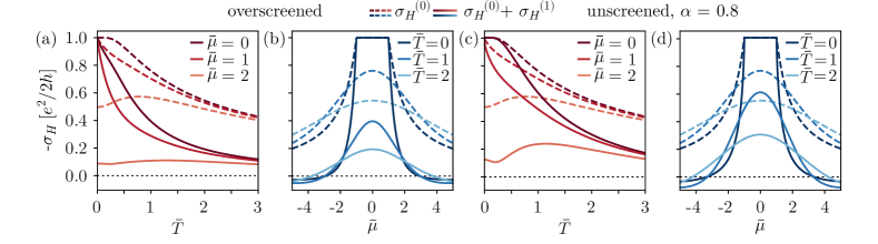
Figure S1: A comparison between the non-interacting ($\sigma_{H}^{(0)}$, dashed lines) and full ($\sigma_{H}=\sigma_{H}^{(0)}+\sigma_{H}^{(1)}$, solid lines) Hall conductivities. Panels (a) Curves are shown as a function of temperature for fixed values of the chemical potential when the Coulomb interaction is heavily screened. Panel (b) Same as Panel (a), but as a function of chemical potential and for fixed values of temperature. Panels (c) and (d) Curves corresponding to (a) and (b), for an unscreened interaction with $\alpha=0.8$.

References

• [1]
• [2]
• Thouless et al. [1982] D. J. Thouless, M. Kohmoto, M. P. Nightingale, and M. den Nijs, Quantized hall conductance in a two-dimensional periodic potential, Physical review letters 49, 405 (1982).
• Xiao et al. [2010] D. Xiao, M.-C. Chang, and Q. Niu, Berry phase effects on electronic properties, Reviews of modern physics 82, 1959 (2010).
• Coleman and Hill [1985] S. Coleman and B. Hill, No more corrections to the topological mass term in qed3, Physics Letters B 159, 184 (1985).
• Zhang and Zubkov [2020] C. Zhang and M. Zubkov, Influence of interactions on the anomalous quantum hall effect, Journal of Physics A: Mathematical and Theoretical 53, 195002 (2020).
• Haldane [1988] F. D. M. Haldane, Model for a quantum hall effect without landau levels: Condensed-matter realization of the” parity anomaly”, Physical review letters 61, 2015 (1988).
• Lai and Hung [2014] H.-H. Lai and H.-H. Hung, Effects of short-ranged interactions on the kane-mele model without discrete particle-hole symmetry, Physical Review B 89, 165135 (2014).
• Hankiewicz and Vignale [2006] E. Hankiewicz and G. Vignale, Coulomb corrections to the extrinsic spin-hall effect of a two-dimensional electron gas, Physical Review B 73, 115339 (2006).
• Lee [2011] D.-H. Lee, Effects of interaction on quantum spin hall insulators, Physical Review Letters 107, 166806 (2011).
• Ado et al. [2017] I. Ado, I. Dmitriev, P. Ostrovsky, and M. Titov, Sensitivity of the anomalous hall effect to disorder correlations, Physical Review B 96, 235148 (2017).
• Ado et al. [2015] I. Ado, I. Dmitriev, P. Ostrovsky, and M. Titov, Anomalous hall effect with massive dirac fermions, Europhysics Letters 111, 37004 (2015).
• Giuliani and Vignale [2005] G. Giuliani and G. Vignale, Quantum theory of the electron liquid (Cambridge university press, 2005).
• Note [1] See the supplementary material online for more details.
• Note [2] Since our calculation pertains to a single valley, it only recovers half of the result for the Haldane model.
• Sinitsyn et al. [2006] N. Sinitsyn, J. Hill, H. Min, J. Sinova, and A. MacDonald, Charge and spin hall conductivity in metallic graphene, Physical review letters 97, 106804 (2006).
• Leonforte et al. [2019] L. Leonforte, D. Valenti, B. Spagnolo, A. A. Dubkov, and A. Carollo, Haldane model at finite temperature, Journal of Statistical Mechanics: Theory and Experiment 2019, 094001 (2019).
• Note [3] Note that there are 3 diagrams which we omitted in the main text, namely the RPA and the Hartree self-energy diagrams. The first only contributes to the screening of the external field, while the latter two are cancelled by the positive homogeneous electronic background.
• Peskin [2018] M. E. Peskin, An introduction to quantum field theory (CRC press, 2018).
• Note [4] We note that, since for a contact potential only power divergences are present in the first-order diagrams, dimensional regularisation could be used as well. In that case, none of these divergences would appear, and the final result would be the same.
• González et al. [1994] J. González, F. Guinea, and M. Vozmediano, Non-fermi liquid behavior of electrons in the half-filled honeycomb lattice (a renormalization group approach), Nuclear Physics B 424, 595 (1994).
• Kotov et al. [2008] V. N. Kotov, V. M. Pereira, and B. Uchoa, Polarization charge distribution in gapped graphene: Perturbation theory and exact diagonalization analysis, Physical Review B 78, 075433 (2008).
• Note [5] This is because the Coulomb interaction is mediated by photons, which are much faster than the interacting electrons, thus making the interactions “instantaneous”.
• Sarma et al. [2011] S. D. Sarma, S. Adam, E. Hwang, and E. Rossi, Electronic transport in two-dimensional graphene, Reviews of modern physics 83, 407 (2011).
• Zhou et al. [2007] S. Y. Zhou, G.-H. Gweon, A. Fedorov, d. First, PN, W. De Heer, D.-H. Lee, F. Guinea, A. Castro Neto, and A. Lanzara, Substrate-induced bandgap opening in epitaxial graphene, Nature materials 6, 770 (2007).
• Wang et al. [2015] Z. Wang, C. Tang, R. Sachs, Y. Barlas, and J. Shi, Proximity-induced ferromagnetism in graphene revealed by the anomalous hall effect, Physical review letters 114, 016603 (2015).
• Mak et al. [2014] K. F. Mak, K. L. McGill, J. Park, and P. L. McEuen, The valley hall effect in mos2 transistors, Science 344, 1489 (2014).
• Sinova et al. [2015] J. Sinova, S. O. Valenzuela, J. Wunderlich, C. Back, and T. Jungwirth, Spin hall effects, Reviews of modern physics 87, 1213 (2015).
• Kane and Mele [2005] C. L. Kane and E. J. Mele, Quantum spin hall effect in graphene, Physical review letters 95, 226801 (2005).
• Choi et al. [2023] Y.-G. Choi, D. Jo, K.-H. Ko, D. Go, K.-H. Kim, H. G. Park, C. Kim, B.-C. Min, G.-M. Choi, and H.-W. Lee, Observation of the orbital hall effect in a light metal ti, Nature 619, 52 (2023).
• Bhowal and Vignale [2021] S. Bhowal and G. Vignale, Orbital hall effect as an alternative to valley hall effect in gapped graphene, Physical Review B 103, 195309 (2021).