Accurate and Honest Approximation of Correlated Qubit Noise

Abstract

Accurate modeling of noise in realistic quantum processors is critical for constructing fault-tolerant quantum computers. While a full simulation of actual noisy quantum circuits provides information about correlated noise among all qubits and is therefore accurate, it is, however, computationally expensive as it requires resources that grow exponentially with the number of qubits. In this paper, we propose an efficient systematic construction of approximate noise channels, where their accuracy can be enhanced by incorporating noise components with higher qubit-qubit correlation degree. To formulate such approximate channels, we first present a method, dubbed the cluster expansion approach, to decompose the Lindbladian generator of an actual Markovian noise channel into components based on interqubit correlation degree. We then generate a $k$-th order approximate noise channel by truncating the cluster expansion and incorporating noise components with correlations up to the $k$-th degree. We require that the approximate noise channels must be accurate and also “honest”, i.e., the actual errors are not underestimated in our physical models. As an example application, we apply our method to model noise in a three-qubit quantum processor that stabilizes a $\llbracket 2,0,0\rrbracket$ codeword, which is one of the four Bell states. We find that, for realistic noise strength typical for fixed-frequency superconducting qubits coupled via always-on static interactions, correlated noise beyond two-qubit correlation can significantly affect the code simulation accuracy. Since our approach provides a systematic noise characterization, it enables the potential for accurate, honest and scalable approximation to simulate large numbers of qubits from full modeling or experimental characterizations of small enough quantum subsystems, which are efficient but still retain essential noise features of the entire device.

I Introduction

Noise presents the major stumbling block in constructing a scalable quantum information processing device. To protect quantum information against noise such that error rates are small enough for practical quantum advantage in large-scale quantum processors, one needs to implement quantum error correction (QEC) [1, 2, 3, 4], where a logical qubit is encoded using many physical qubits. The basic idea behind QEC is that the logical error rate can be made arbitrarily small by increasing the number of physical qubits provided that the physical-qubit error rate is below a certain threshold [5, 6, 7, 8]. Since the assessment of QEC performance is based on the assumption of the underlying noise model, accurate noise modelings and characterizations of quantum processors are absolutely essential for designing reliable and practical QEC. Moreover, faithful information on noise in realistic quantum devices is also crucial for devising more noise-resilient qubit architectures and hardware-efficient QEC codes with better threshold and smaller overhead. For example, for devices with biased Pauli noise, cat qubits [9, 10, 11] and the XZZX surface code [12] are favorable as they possess outstanding resilience against such noise.

Knowledge about noise in quantum devices can be obtained by doing full simulations or experimental characterizations, e.g., gate set [13, 14, 15], quantum state and process tomography [16, 17], Lindblad tomography [18] or randomized benchmarking [19, 20], of the actual physical device, which supply details on the qubit state at a given moment or quantum process/channel due to a gate application of a certain duration. Such theoretical simulations or experimental characterizations, however, require computational or experimental resources (such as number of measurements) that scale exponentially with the number of qubits, which makes them impractical for large quantum circuits. The question that naturally arises is how can one use the full characterization of noise in small quantum processors to accurately assess the performance of large quantum information processors?

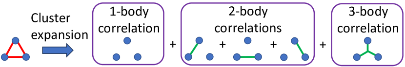
Figure 1: Schematics of the cluster expansion approach, a perturbative series method that decomposes the Lindbladian (noise generator) into terms based on the interqubit correlation degrees. Shown is an example of the cluster expansion approach applied to noise in a three-qubit quantum processor with triangular connectivity.

One strategy used to simulate noise in large quantum systems is to assume a Pauli noise model [21, 22, 23] and construct approximate stochastic noise channels based on the Pauli twirling approximation [24, 25] which averages the noise channels with respect to a set of unitaries. This oversimplified model, however, often does not provide an accurate and honest description of noise in real quantum systems as it does not capture coherent noise and non-Pauli errors such as pulse miscalibration, leakage, etc, which are the dominant noise in many realistic quantum devices. In this paper, we propose a general systematic approach to generate approximate noise channels beyond the Pauli noise model, which is based on actual noise data obtained from either realistic simulations or experimental characterizations of subsystems of the quantum device. In particular, we consider obtaining the actual noise data via either Lindbladian dynamics simulation or experimental characterizations such as Lindblad tomography [18], process tomography [17] which supplies data that can be fitted to get the best-fit Lindbladian for the quantum channel [26, 27], etc.; here we focus on the former, i.e., using inputs from theoretical simulations.

We present an approach, dubbed the cluster expansion method, to decompose the actual noise into components according to their degree of qubit-qubit correlations [see Fig. 1]. A $k$-th order approximate noise channel is then generated by truncating the expansion and including noise components with qubit-qubit correlations up to the $k$-th degree. The accuracy of the approximate noise model can be improved (at the expense of reducing the efficiency) by including noise components with increasingly higher interqubit correlation degree. Further, we impose that our approximate noise channel must be constructed in an “honest” manner, i.e., the approximate error does not underestimate the actual error. Therefore, the aim of this paper is to provide a systematic method to construct approximate noise models, $\mathcal{N}_{\mathrm{approx}}$, such that

1. The action of $\mathcal{N}_{\mathrm{approx}}$ can be made as “accurate” (faithful) as possible in representing the action of the actual channel $\mathcal{N}_{\mathrm{actual}}$,

2. $\mathcal{N}_{\mathrm{approx}}$ gives an “honest” representation of the noise in the actual system, and

3. The construction of $\mathcal{N}_{\mathrm{approx}}$ is scalable in the number of qubits.

This paper is organized as follows. In Sec. II, we begin by giving a short review of the Lindblad master equation and also define the normal-form of a noise channel. Subsequently in Sec. III, we use the cluster expansion approach to decompose the Lindbladian into terms based on their qubit-qubit correlation degrees. In Sec. IV, we present ways to construct approximate noise channels using the decomposed Lindbladians and define the honesty and accuracy criteria of the approximate noise models. We then give a detailed application of our noise model for QEC in Sec. V, focusing on a specific example, namely the $\llbracket 2,0,0\rrbracket$ code. We give the conclusion in Sec. VI. The appendices contain details on the superoperator representation, example applications of the cluster expansion method, and results for simulating the $\llbracket 2,0,0\rrbracket$ code in a three-qubit quantum processor with triangular connectivity.

II Lindblad noise model

We assume that the evolution of a quantum processor interacting with its environment is well approximated by the Lindblad master equation [28, 29]:

$$\frac{d\rho(t)}{dt}=\mathcal{L}\rho(t),$$ (1)

where $\rho$ is the system density matrix and the Lindbladian $\mathcal{L}$ is given by [28, 29]

$$\mathcal{L}(\rho)=-i[\hat{H},\rho]+\sum_{j}\gamma_{j}\left(\hat{A}_{j}\rho\hat{A}_{j}^{\dagger}-\frac{1}{2}\hat{A}_{j}^{\dagger}\hat{A}_{j}\rho-\frac{1}{2}\rho\hat{A}_{j}^{\dagger}\hat{A}_{j}\right),$$ (2)

with $[\cdot,\cdot]$ denoting the commutator. Here the Hamiltonian $\hat{H}$ describes the unitary dynamics of the system, which can include coherent errors resulting from pulse miscalibration, crosstalk due to always-on qubit-qubit interactions, etc. $\hat{A}_{j}$ is the Lindblad (jump) operator with a jump/dissipation rate $\gamma_{j}$ representing the incoherent noise (e.g., dephasing and relaxation) due to the interaction between the system and the environment. The resulting channel (propagator) that evolves the system for a duration $t$ can be written as

$$\mathcal{V}=\hat{T}\left[\exp\left(\int_{0}^{t}\mathcal{\mathcal{L}}(t^{\prime})dt^{\prime}\right)\right],$$ (3)

where $\hat{T}$ denotes the time-ordering operator.

In order to describe the dynamics due to only the unwanted noise, we write the channel (propagator) in the normal form. This normal form is defined as the noise channel with the unitary dynamics contribution $\mathcal{U}^{\dagger}$ of the ideal Hamiltonian being factored out, i.e.,

$$\mathcal{N}=\mathcal{V}\circ\mathcal{U}^{\dagger},$$ (4)

where $\mathcal{U}^{\dagger}(\rho)=U^{\dagger}\rho U$ is the ideal (noiseless) channel with $U$ being the ideal target unitary operator .

If the Hamiltonian or Lindblad operators are time-dependent then the Lindbladian $\mathcal{L}$ and hence, the noise channel are also time-dependent. We capture the effect of this time-dependent dynamics by using $\widetilde{\mathcal{L}}$, which is an effective dimensionless time-independent Lindbladian that serves as a generator for the system evolution from the beginning to the end of the application of the noise channel. In the superoperator representation (see Appendix A), it is given by

$$\hat{\widetilde{\mathcal{L}}}=\mathrm{ln}(\hat{\mathcal{N}}),$$ (6)

where $\hat{\widetilde{\mathcal{L}}}$ is the superoperator representation of the Lindbladian $\widetilde{\mathcal{L}}$ and $\hat{\mathcal{N}}$ is the superoperator representation of the normal-form noise channel $\mathcal{N}$ as defined in Eq. (4). In general, the matrix logarithm in Eq. (6) yields an infinite number of branch cuts. However, for small enough noise strength, the normal-form noise channel is close to the identity channel and hence the zeroth branch cut of the matrix logarithm taken in Eq. (6) gives a physical Lindbladian, i.e., the Lindbladian where all its eigenvalues have non-positive real parts.

III Lindbladian Decomposition using Cluster Expansion

Quantum circuits are usually transpiled into one- and two-qubit gates. Noise associated with the gate operations are then expected to have significant effect only in the neighborhood of the qubits where the gates are applied. As a result, we can simplify the noise model by first decomposing the noise into locally correlated noise and incorporating only the subset of noise that substantially affects the gates performance.

To separate and characterize the contributions due to noise with different degree of correlations, we present a method akin to the cluster expansion approach [31, 32] used for interacting closed many-body systems. The cluster expansion approach is a perturbative series expansion which sums over the contribution from clusters with different size; see Fig. 1. Instead of doing a power-series expansion over the partition function as in the standard cluster expansion approach used to treat the interactions in closed many-body systems [31, 32], our cluster expansion approach decomposes the Lindblad generator $\hat{\widetilde{\mathcal{L}}}$ of an actual noise channel into sum of components with different degree of qubit-qubit correlations, i.e.,

$$\hat{\widetilde{\mathcal{L}}}=\hat{\widetilde{\mathcal{L}}}^{1-\mathrm{body}}+\hat{\widetilde{\mathcal{L}}}^{2-\mathrm{body}}+\cdots+\hat{\widetilde{\mathcal{L}}}^{n-\mathrm{body}},$$ (7)

where $\hat{\widetilde{\mathcal{L}}}$ denotes the exact Lindbladian of the whole system which comprises $n$ number of qubits. Here,

$$\hat{\widetilde{\mathcal{L}}}^{m-\mathrm{body}} =\sum_{S_{m}}\hat{\widetilde{\mathcal{L}}}^{S_{m}}$$ (8)

is the component of the Lindbladian that describes noise with $m$-th correlation degree. The sum used to evaluate the $m$-th order correlated Lindbladian $\hat{\widetilde{\mathcal{L}}}^{m-\mathrm{body}}$ in Eq. (8) is performed over all subsets of size $m$ in the set $S=\{1,2,\cdots,n\}$, i.e., $S_{m}\subseteq S$ such that $|S_{m}|=m$. Each of the $m$-th order correlated noise terms is given by the following recurrence relation:

$$\hat{\widetilde{\mathcal{L}}}^{S_{m}} =\mathrm{ln}\left(\mathrm{Tr}_{\bar{S}_{m}}\left[e^{\hat{\widetilde{\mathcal{L}}}}\left(\mathds{1}_{S_{m}}\otimes\rho_{\bar{S}_{m}}\right)\right]\otimes\mathds{1}_{\bar{S}_{m}}\right)-\sum_{R\subsetneq S_{m}}\hat{\widetilde{\mathcal{L}}}^{R}$$

$$=\mathrm{ln}\left(\mathrm{Tr}_{\bar{S}_{m}}\left[e^{\hat{\widetilde{\mathcal{L}}}}\left(\mathds{1}_{S_{m}}\otimes\frac{\mathds{1}_{\bar{S}_{m}}}{|\mathcal{H}_{\bar{S}_{m}}|}\right)\right]\otimes\mathds{1}_{\bar{S}_{m}}\right)$$

$$\hskip 14.22636pt-\sum_{R\subsetneq S_{m}}\hat{\widetilde{\mathcal{L}}}^{R},$$ (9)

where $\bar{S}_{m}=\{x\in S:x\notin S_{m}\}$ denotes the complement subset of $S_{m}$. As shown in Eq. (III), $\hat{\widetilde{\mathcal{L}}}^{S_{m}}$ is calculated by first doing a partial trace of the whole system ($n$-qubits) noise channel over the $(n-m)$ qubits which live in the Hilbert space $\mathcal{H}_{\bar{S}_{m}}$ with dimension $|\mathcal{H}_{\bar{S}_{m}}|={n_{\mathrm{qlvl}}}^{(n-m)}$. We use ${n_{\mathrm{qlvl}}}$ to denote the number of the qubit states, where ${n_{\mathrm{qlvl}}}=2$ for the case considered in this paper. Here, the state of the ($n-m$) qubits is taken to be a fully mixed state; this is a valid assumption for QEC circuits, the focus of our paper, as noise in data qubits makes the syndrome qubits undergoing ergodic evolutions into all possible states. The tensor product with the identity ($\mathds{1}_{\bar{S}_{m}}$) in the $(n-m)$-qubit subspace after the trace operation is to ensure that the dimension of the noise channel is the same as its initial dimension. Afterward, we take the logarithm of the resulting noise channel to get the effective Lindbladian that describes noise in $m$-qubits subsystem where it includes all noise components with correlation degrees up to the $m$-th order. Subsequently, to get the $m$-th order correlated noise term $\hat{\widetilde{\mathcal{L}}}^{S_{m}}$, we subtract from the resulting expression all the lower ($m^{\prime}<m$)-th order correlated noise terms, where the subtraction is over all proper subsets of $S_{m}$ ($R\subsetneq S_{m}$), i.e., all subsets of $S_{m}$ that are not equal to $S_{m}$.

IV Approximate Noise Model

IV.1 Construction

Using the above decomposed Lindbladians, we can now ask the question: can we truncate the total Lindblad term $\hat{\widetilde{\mathcal{L}}}$ by considering only terms up to the $k$-th order, where $k\leq n$? As we show in the rest of this work, we answer this in the affirmative. Specifically, we consider the $k$-body approximation of the Lindbladian $\hat{\widetilde{\mathcal{L}}}_{k}$ by ignoring all higher-order terms ($m>k$), defining:

$$\hat{\widetilde{\mathcal{L}}}_{k}=\hat{\widetilde{\mathcal{L}}}^{1-\mathrm{body}}+\hat{\widetilde{\mathcal{L}}}^{2-\mathrm{body}}+\cdots+\hat{\widetilde{\mathcal{L}}}^{k-\mathrm{body}}.$$ (10)

We remark that, in general, each term in $\hat{\widetilde{\mathcal{L}}}_{k}$ and therefore $\hat{\widetilde{\mathcal{L}}}_{k}$ is not guaranteed to be a physical Lindbladian, as it comprises a sum of both positive and negative Lindblad terms [see Eqs. (8) and (III)] . However, all the 1-body terms $\hat{\widetilde{\mathcal{L}}}^{S_{1}}$ and hence $\hat{\widetilde{\mathcal{L}}}^{1-\mathrm{body}}$ are guaranteed to be physical Lindbladians. Note that the way we calculate each term in $\hat{\widetilde{\mathcal{L}}}_{k}$, as defined in Eqs. (8) and (III), guarantees that the summation in Eq. (10) does not over- or under-count the expected error, as we showcase with several examples in Appendix B.

To generate the approximate noise channel, we can in principle exponentiate the $k$-body approximate Lindbladian $\hat{\widetilde{\mathcal{L}}}_{k}$. However, for sufficiently small noise strength, we can further simplify the computation for the approximate noise channel by making a Trotter approximation. Combining the truncation of the Lindbladian cluster-expansion and the Trotter approximation, we write the $k$-th order approximate noise channel as

$$\hat{\mathcal{N}}_{\mathrm{approx},k}(g)\equiv\prod_{S_{1}}\exp(g\hat{\widetilde{\mathcal{L}}}^{S_{1}})\cdots\prod_{S_{k}}\exp(g\hat{\widetilde{\mathcal{L}}}^{S_{k}}),$$ (11)

where $g$ is the gain factor , a free parameter to be optimized in order to make the approximation “honest” and as accurate as possible (see Sec. IV.2 for details on the honesty and accuracy criteria). We use this Trotterized form in what follows as it allows us to reason about noise in the context of more complex quantum circuits, where each noise component can be replaced by a quantum operation occurring over a subset $S_{m}$ with $m\leq k$.

We note that Our approximate noise model can be scaled to larger systems even when there is crosstalk between all connected pairs of qubits as long as the number of qubits that the gates act on are small enough. This is because the cluster expansion can be truncated at a certain depth where the small amplitude of higher-order terms, i.e., terms with correlation degree greater than $k$, allows us to entirely neglect these higher-order residual errors.

IV.2 Honesty and accuracy

To characterize the performance of the approximate noise model, we calculate the distances between ideal (noiseless), actual, and approximate noise channels, which quantify the distinguishability between the channels. Based on these distances, we can characterize two properties of the approximate noise channels: honesty and accuracy [35, 36, 37].

An approximate noise channel is honest if it does not underestimate the deleterious effect of the actual noise. On the other hand, the accuracy of an approximate channel refers to how closely it can emulate the impact of the actual noise. More explicitly, if we consider the ideal (noiseless) $\mathcal{V}_{\mathrm{ideal}}$, actual $\mathcal{V}_{\mathrm{actual}}$, and approximate $\mathcal{V}_{\mathrm{approx}}$ target channels map an initial pure state $|\Psi_{\mathrm{in}}\rangle$ into the $\rho_{\mathrm{ideal}}$, $\rho_{\mathrm{actual}}$, and $\rho_{\mathrm{approx}}$ density matrices, respectively, we can then define the honesty and accuracy criteria of the approximate noise channel $\mathcal{V}_{\mathrm{approx}}$ in terms of the distance metrics $\mathcal{D}$ between these density matrices as

$$\mathrm{honest\,if\hskip 5.69046pt} \frac{\mathcal{D}(\rho_{\mathrm{ideal}},\rho_{\mathrm{approx}})}{\mathcal{D}(\rho_{\mathrm{ideal}},\rho_{\mathrm{actual}})}\geq 1,$$ (12)

$$\mathrm{accurate\,if\hskip 5.69046pt\,} \frac{\mathcal{D}(\rho_{\mathrm{ideal}},\rho_{\mathrm{actual}})}{\mathcal{D}(\rho_{\mathrm{actual}},\rho_{\mathrm{approx}})}\geq 1,$$ (13)

for every input pure state $|\Psi_{\mathrm{in}}\rangle$.

For ease of understanding, we show in Fig. 2 the schematics of the honesty and accuracy criteria of approximate noise models. For the approximate noise model to be honest, its density matrix must lie outside the ball whose radius is defined by the distance between $\rho_{\mathrm{ideal}}$ and $\rho_{\mathrm{actual}}$ (the shaded ball shown in Fig. 2). On the other hand, for the approximate noise model to be accurate, it must be as close as possible to the actual model; in other words, the distance between them (the green dashed line in Fig. 2) must be as small as possible. So, accurate and honest approximate noise models must lie on the green arc outside the shaded ball but close to the actual model.

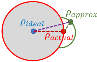
Figure 2: A schematic of distances between density matrices obtained from the ideal ($\rho_{\mathrm{ideal}}$), actual ($\rho_{\mathrm{actual}}$) and approximate ($\rho_{\mathrm{approx}}$) models. Shaded area represents parameter regimes where approximate noise models are not honest. Honest approximate noise models must lie outside the ball defined by the distance between the ideal and actual models (shown by shaded ball). For the approximate noise models to be accurate, they must be close to the actual model.

To obtain the best approximate noise model, we find the optimal gain factor ($g=g_{\mathrm{opt}}$) in $\hat{\mathcal{N}}_{\mathrm{approx}}$ [Eq. (11)] that yields the highest state-averaged accuracy ratio, i.e.,

$$\max_{g}\left\langle\frac{D(\rho_{\mathrm{ideal}},\rho_{\mathrm{actual}})}{D(\rho_{\mathrm{actual}},\rho_{\mathrm{approx}}(g))}\right\rangle_{|\Psi_{\mathrm{in}}\rangle},$$

subject to the honesty constraint [Eq. (12)]. Here, $\langle\cdots\rangle_{|\Psi_{\mathrm{in}}\rangle}$ denotes the averaging over all the pure input states (for the case of QEC, which is the focus of our paper, these input states are the stabilizer states of the QEC code).

V Application to QEC: $\llbracket 2,0,0\rrbracket$ code

V.1 Basics of $\llbracket 2,0,0\rrbracket$ code

As an example application of our noise model, we consider applying it to the simplest QEC code, the $\llbracket 2,0,0\rrbracket$ code. As its name suggests, this code has 2 physical qubits, zero logical qubits and zero distance. It has zero logical qubits since the number of stabilizers ($XX$ and $ZZ$) is the same as the number of physical data qubits. As it does not have any logical operators, it has zero distance, which means that it cannot correct any physical errors.

The circuit for implementing the $\llbracket 2,0,0\rrbracket$ code is shown in Fig. 3. The input state of the circuit is taken to be any one of the four Bell states, where each of them has a unique syndrome measurement at each round of the implementation of an ideal (noiseless) $\llbracket 2,0,0\rrbracket$-code circuit, as shown in Table 1.

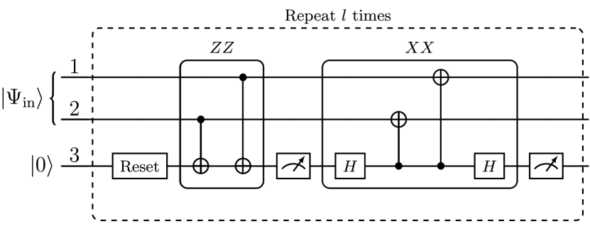
Figure 3: Quantum circuit for implementing the $\llbracket 2,0,0\rrbracket$ code. The code consists of two data qubits (qubits 1 and 2) and one syndrome qubit (qubit 3). The input state of the data qubits $|\Psi_{\mathrm{in}}\rangle$ is one of the Bell states while the syndrome qubit is initialized in state $|0\rangle$. The syndrome qubit is reset to $|0\rangle$ at the beginning of each round of the implementation of the $\llbracket 2,0,0\rrbracket$ code. The code has 2 stabilizers: $ZZ$ and $XX$. The $ZZ$ and $XX$ syndrome measurements of each input Bell state $|\Psi_{\mathrm{in}}\rangle$ for each round of the implementation of an ideal (noiseless) $\llbracket 2,0,0\rrbracket$-code circuit are shown in Table 1.

Input state $|\Psi_{\mathrm{in}}\rangle$	($ZZ$, $XX$) syndrome
$\dfrac{|00\rangle+|11\rangle}{\sqrt{2}}$	(0,0)
$\dfrac{|00\rangle-|11\rangle}{\sqrt{2}}$	(0,1)
$\dfrac{|01\rangle-|10\rangle}{\sqrt{2}}$	(1,0)
$\dfrac{|01\rangle+|10\rangle}{\sqrt{2}}$	(1,1)

Table 1: Data-qubits input states together with the syndrome measurement results of the ancilla qubit at each round of the implementation of an ideal (noiseless) $\llbracket 2,0,0\rrbracket$-code circuit.

V.2 Infidelity distance measure between different quantum channels

Since noise in different quantum channels change the same initial data-qubits states into different quantum states, we can characterize noise in different quantum channels by first defining the fidelity between the data-qubits states resulting from two different quantum channels $\mathcal{E}$ and $\mathcal{F}$ as [38, 39]

$$F_{\mathrm{q}}(\rho_{\mathcal{E}},\rho_{\mathcal{F}})=\left[\mathrm{Tr}\left(\sqrt{\sqrt{\rho_{\mathcal{E}}}\rho_{\mathcal{F}}\sqrt{\rho_{\mathcal{E}}}}\right)\right]^{2}.$$ (14)

As different data-qubits states give rise to different probabilities of the syndrome-qubit measurement results $x$, we can similarly define the fidelity of the syndrome qubit measurements of different quantum channels in terms of their syndrome measurement probabilities [$p_{\mathcal{E}}(x)$ and $p_{\mathcal{F}}(x)$] as [39]

$$F_{\mathrm{c}}(p_{\mathcal{E}},p_{\mathcal{F}})=\left[\sum_{x}\sqrt{p_{\mathcal{E}}(x)p_{\mathcal{F}}(x)}\right]^{2}.$$ (15)

Combining the fidelity measures characterized in terms of the data-qubits states and syndrome qubit measurements, we can define the infidelity distance between any two quantum channels used to implement QEC codes as

$$D^{\mathrm{inf}}_{|\Psi_{\mathrm{in}}\rangle}(\rho_{\mathcal{E}},\rho_{\mathcal{F}})=1-\left(\sum_{x\in\{0,1\}^{2l}}\bigg{[}\sqrt{p_{\mathcal{E}}(x|\Psi_{\mathrm{in}})p_{\mathcal{F}}(x|\Psi_{\mathrm{in}})}\times\mathrm{Tr}\left(\sqrt{\sqrt{\rho_{\mathcal{E}}(x|\Psi_{\mathrm{in}})}\rho_{\mathcal{F}}(x|\Psi_{\mathrm{in}})\sqrt{\rho_{\mathcal{E}}(x|\Psi_{\mathrm{in}})}}\right)\bigg{]}\right)^{2},$$ (16)

where $x\in\{0,1\}^{2l}$ are the syndrome measurement bit strings after the $l$-th round implementation of the $\llbracket 2,0,0\rrbracket$-code circuit and $|\Psi_{\mathrm{in}}\rangle$ is the data-qubits input state, which is one of the four Bell states. Here, $\rho_{\mathcal{E},\mathcal{F}}(x|\Psi_{\mathrm{in}})$ are the data-qubits density matrices resulting from the application of the quantum channels $\mathcal{E}$ and $\mathcal{F}$, respectively. The density matrices $\rho_{\mathcal{E},\mathcal{F}}(x|\Psi_{\mathrm{in}})$ are associated with the probability distributions $p_{\mathcal{E},\mathcal{F}}(x|\Psi_{\mathrm{in}})$ of a given syndrome measurement result $x$ given a particular input state $|\Psi_{\mathrm{in}}\rangle$. The infidelity values are given by $0\leq D^{\mathrm{inf}}_{|\Psi_{\mathrm{in}}\rangle}(\rho_{\mathcal{E}},\rho_{\mathcal{F}})\leq 1$, where $D^{\mathrm{inf}}_{|\Psi_{\mathrm{in}}\rangle}(\rho_{\mathcal{E}},\rho_{\mathcal{F}})=0$ means that the two density matrices are identical and $D^{\mathrm{inf}}_{|\Psi_{\mathrm{in}}\rangle}(\rho_{\mathcal{E}},\rho_{\mathcal{F}})=1$ indicates that the two density matrices are furthest apart from each other.

In the context of QEC, the honesty and accuracy criteria [Eqs. (12) and (13)] of our approximate noise models can then be defined in terms of the infidelity metrics given in Eq. (16). Specifically, we require these criteria to be satisfied for every input pure state $|\Psi_{\mathrm{in}}\rangle$ in the logical space spanned by the stabilizer states (which are the four Bell states for our example of the $\llbracket 2,0,0\rrbracket$ code).

V.3 Simulation

We now analyze the implementation of our noise model for the $\llbracket 2,0,0\rrbracket$ code in a concrete physical setup: a quantum processor consisting of fixed-frequency qubits coupled to each other via static transverse couplings. The system Hamiltonian is given by

$$\hat{H}(t)=\hat{H}_{q}+\hat{H}_{\mathrm{int}}+\hat{H}_{\mathrm{dr}}(t),$$ (17)

where $\hat{H}_{q}$ is the bare qubit Hamiltonian, $\hat{H}_{\mathrm{int}}$ is the qubit-qubit interaction term and $\hat{H}_{\mathrm{dr}}(t)$ is the qubit drive term.

We consider the qubits to be a collection of two-level systems with the bare Hamiltonian (in units $\hbar=1$)

$$\hat{H}_{q}=\sum_{j}\frac{\omega_{q_{j}}}{2}\hat{\sigma}_{z,j},$$ (18)

where $\hat{\sigma}_{z,j}=|0\rangle_{j}{}_{j}\langle 0|-|1\rangle_{j}{}_{j}\langle 1|$ is the $j$-th qubit Pauli-$z$ operator and $\omega_{q_{j}}$ is the $j$-th qubit frequency. The qubits are coupled to each other via always-on static transverse couplings with the Hamiltonian

$$\hat{H}_{\mathrm{int}}=\sum_{\langle j,k\rangle}J_{jk}(\hat{\sigma}_{+,j}\hat{\sigma}_{-,k}+\hat{\sigma}_{+,k}\hat{\sigma}_{-,j}),$$ (19)

where the sum is over all pairs of interacting qubits. Here, $J_{jk}$ is the strength of the coupling between qubits $j$ and $k$, $\hat{\sigma}_{+}=|1\rangle\langle 0|$ and $\hat{\sigma}_{-}=|0\rangle\langle 1|$ are the qubit raising and lowering operators, respectively. We consider two different connectivities: linear and triangle geometries (see Fig. 4), where the linear geometry has one less qubit-qubit coupling compared to the triangle geometry.

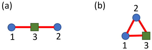
Figure 4: Connectivities of the 3-qubit processor used for implementing the $\llbracket 2,0,0\rrbracket$ code: (a) Linear and (b) Triangle geometry. Circles represent data qubits and squares represent syndrome qubits. Numbers indicate the qubit labels as in Fig. 3.

Gates are implemented by driving the qubits with control fields where the drive Hamiltonian is

$$\hat{H}_{\mathrm{dr}}(t) =\sum_{\begin{subarray}{c}j\in\mathrm{driven}\\ \mathrm{qubits}\end{subarray}}\Omega_{\mathrm{dr},j}(t)\left(\hat{\sigma}_{+,j}e^{-i(\omega_{\mathrm{dr},j}t+\phi_{\mathrm{dr},j})}+\mathrm{H.c.}\right),$$ (20)

where $\Omega_{\mathrm{dr},j}(t)$, $\omega_{\mathrm{dr},j}$ and $\phi_{\mathrm{dr},j}$ are respectively the envelope, frequency and phase of the control field that drives qubit $j$. The notation “H.c.” denotes the Hermitian conjugate of the preceding term. A single-qubit gate is implemented by driving the qubit with a control field at the qubit’s characteristic frequency. Any single-qubit gate can be implemented in this way by choosing appropriate amplitude, duration and phase of the driving pulse. However, here we choose to realize single-qubit gates using sequences of $X$ and $Y$ rotations obtained using the $X$-$Y$ decomposition [39] of the gates. The two-qubit (CNOT) gate used in our simulation is a cross-resonance [40, 41] gate which is implemented by driving the control qubit at the frequency of the target qubit. To cancel the unwanted effect due to crosstalk in the cross-resonance gate, we apply an echoed version of the calibrated pulse sequence as described in Ref. [42].

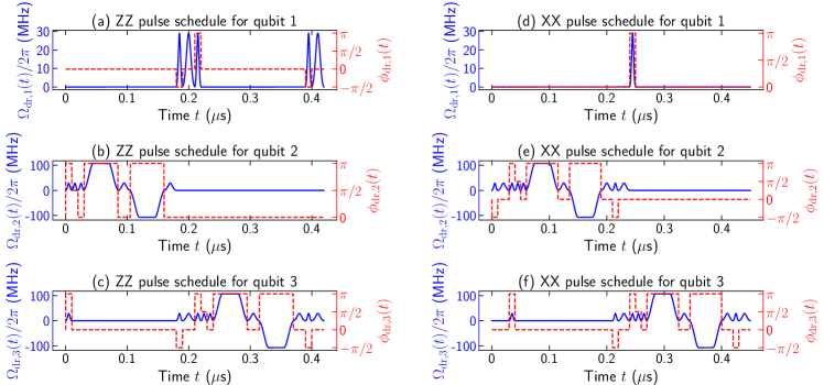
Figure 5: Amplitudes $\Omega_{\mathrm{dr},j}(t)$ and phases $\phi_{\mathrm{dr},j}(t)$ of the control pulses for the $ZZ$ [panels (a), (b), and (c)] and $XX$ [panels (d), (e), and (f)] stabilizers of the $\llbracket 2,0,0\rrbracket$ code implemented in a linear geometry. From top to bottom: pulse schedules for qubit $j=1,2,3$ (the qubit labels are the same as those in Fig. 3).

The pulse schedules of the $ZZ$ and $XX$ stabilizers, which consist of single- and two-qubit gate pulses, are shown in the left and right panels of Fig. 5, respectively; here we choose Gaussian and Gaussian-square pulse envelopes. These pulse schedules are for a linearly-connected qubit geometry (the pulse schedules for the triangle geometry are not shown as they are similar to those for the linear geometry). These pulse schedules are calibrated for the qubit parameters shown in Table 2, where we use values typical for fixed-frequency superconducting qubits. For the linear geometry, our calibrated pulses yield average fidelities of $0.9896$ and $0.9888$ for the $ZZ$ and $XX$ stabilizers, respectively. Similar calibrated pulses for the triangle geometry yield average fidelities of $0.9870$ and $0.9832$ for the $ZZ$ and $XX$ stabilizers, respectively.

Qubit frequencies	Qubit-qubit couplings
$\omega_{q_{1}}/2\pi$ = 4.8 GHz	$J_{1,2}/2\pi$ = 4 MHz (Triangle)
	= 0 (Linear)
$\omega_{q_{2}}/2\pi$ = 5.2 GHz	$J_{2,3}/2\pi$ = 4 MHz
$\omega_{q_{3}}/2\pi$ = 5 GHz	$J_{1,3}/2\pi$ = 4 MHz
Relaxation times	Dephasing times
$T_{1,1}$ = 100 $\mu$s	$T_{\varphi,1}$ = 200 $\mu$s
$T_{1,2}$ = 100 $\mu$s	$T_{\varphi,2}$ = 200 $\mu$s
$T_{1,3}$ = 100 $\mu$s	$T_{\varphi,3}$ = 200 $\mu$s

Table 2: Qubit parameters: qubit frequencies $\omega_{q}$, qubit-qubit coupling strengths $J$, relaxation times $T_{1}$ and pure dephasing times $T_{\varphi}$.

To simulate the gate dynamics which incorporates the effects of dissipation due to $T_{\varphi}$ dephasing and $T_{1}$ relaxation, we use the Lindblad master equation:

$$\frac{d\rho(t)}{dt} =-i[\hat{H}(t),\rho(t)]+\sum_{j}\frac{1}{T_{\varphi,j}}\bigg{(}\hat{\sigma}_{z,j}\rho(t)\hat{\sigma}_{z,j}-\rho(t)\bigg{)}$$

$$\hskip 5.69046pt+\sum_{j}\frac{1}{T_{1,j}}\left(\hat{\sigma}_{-,j}\rho(t)\hat{\sigma}_{+,j}-\frac{1}{2}\left\{\hat{\sigma}_{+,j}\hat{\sigma}_{-,j},\rho(t)\right\}\right),$$ (21)

where $\rho(t)$ is the density matrix of the whole system, $T_{\varphi,j}$ and $T_{1,j}$ are the dephasing and relaxation times of qubit $j$, respectively. Here $\{\cdot,\cdot\}$ denotes the anticommutator. The Lindblad master equation simulation in this paper is done using the Python package QuTiP [43, 44].

From the Lindblad master equation simulation, we obtain the actual channel or propagator $\mathcal{V}_{\mathrm{actual}}$ of the $ZZ$ and $XX$ stabilizers which evolve the system from the beginning to the end of each stabilizer’s protocol time. We then convert these propagators into their normal forms $\hat{\mathcal{N}}_{\mathrm{actual}}$ using Eq. (4). Afterward, we convert $\hat{\mathcal{N}}_{\mathrm{actual}}$ into the superoperator form and then take the matrix logarithm of $\hat{\mathcal{N}}_{\mathrm{actual}}$ in order to get the time-independent effective Lindbladians $\hat{\widetilde{\mathcal{L}}}$ [Eq. (6)]. We then decompose these effective Lindbladians $\hat{\widetilde{\mathcal{L}}}$ using the cluster expansion described in Sec. III and exponentiate the decomposed Lindbladians to get the normal-form of the approximate noise channels $\hat{\mathcal{N}}_{\mathrm{approx}}$ as detailed in Sec. IV.1. To convert the approximate noise channels of the $ZZ$ and $XX$ stabilizers into the standard form $\hat{\mathcal{V}}_{\mathrm{approx}}$, we multiply the corresponding $\hat{\mathcal{N}}_{\mathrm{approx}}$ by the ideal (noiseless) target operation $\hat{\mathcal{U}}$, i.e.,

$$\hat{\mathcal{V}}_{\mathrm{approx}}=\hat{\mathcal{N}}_{\mathrm{approx}}\,\hat{\mathcal{U}}.$$ (22)

We use the following procedure to implement the $\llbracket 2,0,0\rrbracket$ code:

1. Choose a Bell state for the input state $|\Psi_{\mathrm{in}}\rangle$ of the data qubits.

2. Reset the syndrome qubit to state $|0\rangle$.

3. Apply a selected error channel, actual $\hat{\mathcal{V}}_{\mathrm{actual}}$ or approximate $\hat{\mathcal{V}}_{\mathrm{approx}}$ (for different gain factors), of the $ZZ$ stabilizer.

4. Apply a noiseless (perfect) projective measurement of the syndrome qubit in the $Z$ basis.

5. Apply a selected error channel, actual $\hat{\mathcal{V}}_{\mathrm{actual}}$ or approximate $\hat{\mathcal{V}}_{\mathrm{approx}}$ (for different gain factors), of the $XX$ stabilizer.

6. Apply a noiseless (perfect) projective measurement of the syndrome qubit in the $Z$ basis.

7. Compute the infidelities between the data-qubits density matrices obtained from the noiseless (ideal) $\hat{\mathcal{V}}_{\mathrm{ideal}}$, actual $\hat{\mathcal{V}}_{\mathrm{actual}}$ and approximate $\hat{\mathcal{V}}_{\mathrm{approx}}$ channels.

8. Repeat steps 2-7.

We apply the above procedure to implement the $\llbracket 2,0,0\rrbracket$ code for two different connectivities: linear and triangle geometries (see Fig. 4). In order to understand the contribution of noise components with different degrees of correlations, for both geometries we perform simulations using two different approximate noise channels: second-order ($\hat{\mathcal{N}}_{\mathrm{approx},2}$) and third-order ($\hat{\mathcal{N}}_{\mathrm{approx},3}$) approximate noise channels [Eq. (11)].

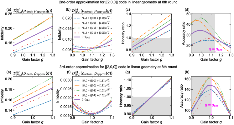
Figure 6: Results simulated for the linear connectivity using the second-order $\hat{\mathcal{N}}_{\mathrm{approx},2}$ [upper panels: (a), (b), (c), and (d)] and third-order $\hat{\mathcal{N}}_{\mathrm{approx},3}$ [lower panels: (e), (f), (g), and (h)] approximate noise channels. They are calculated at the 8th round implementation of the $\llbracket 2,0,0\rrbracket$ code for different input data-qubits states $|\Psi_{\mathrm{in}}\rangle$; the state-averaged results are denoted by $\langle\cdots\rangle_{|\Psi_{\mathrm{in}}\rangle}$ and shown as solid purple lines. (a,b,e,f) Infidelity between the data-qubits density matrices as a function of gain factor $g$: (a,e) Infidelity between ideal and approximate density matrices, (b,f) Infidelity between actual and approximate density matrices. (c,g) Honesty ratio as a function of gain factor $g$. (d,h) Accuracy ratio as a function of gain factor $g$. Magenta arrow denotes $g=g_{\mathrm{opt}}$, i.e., the optimal value of $g$ that maximizes the state-averaged accuracy ratio subject to the honesty constraint [Eq. (12)], where $g_{\mathrm{opt}}\simeq 1.14$ for the second-order and $g=g_{\mathrm{opt}}\simeq 1.0005$ for the third-order approximate channel. Shaded areas in panels (c), (d), (g), and (h) denote regimes where approximate noise models are not honest (honesty ratio $<1$).

V.4 Results and discussion

Figure 6 shows the simulation results for the $\llbracket 2,0,0\rrbracket$ code, computed using the second-order (upper panels) and third-order (lower panels) approximate noise channels. The results shown are for the 8th round implementation of the code in a linear geometry using different input data qubits states $|\Psi_{\mathrm{in}}\rangle$. Figures 6(a) and 6(e) show that the infidelity between the ideal and approximate data-qubits density matrices increases linearly with the gain factor $g$. This is because the gain factor amplifies the noise in the approximate noise channels. Panels (b) and (f) of Fig. 6 show that the infidelities between the resulting actual and approximate data-qubits density matrices $\mathcal{D}^{\mathrm{inf}}_{|\Psi_{\mathrm{in}}\rangle}(\rho_{\mathrm{actual}},\rho_{\mathrm{approx}})$ exhibit a nonmonotonic dependence on the gain factor $g$, where the minimum is at $g\simeq 0.95-1.1$ and $g\simeq 1$ for the second-order and third-order approximate noise channels, respectively.

From these infidelities, we calculate the honesty and accuracy ratios as shown in Figs. 6 (c,g) and 6(d,h), respectively. The honesty ratio increases linearly with the gain factor $g$ where the honesty constraint (honesty ratio $\geq 1$) is satisfied for all the four input Bell states only when $g\gtrsim 1.14$ and $g\gtrsim 1$ for the second-order and third-order approximate channels, respectively. On the other hand, the accuracy ratios have nonmonotonic dependences on the gain factor $g$ with its maximum occurring at $g\simeq 0.95-1.1$ for the second-order approximate noise channel and $g\simeq 1$ for the third-order approximate noise channel. The maximum state-averaged accuracy ratios subject to the honesty constraint are obtained by choosing the optimal $g=g_{\mathrm{opt}}$ in the honesty regime, where $g_{\mathrm{opt}}\simeq 1.14$ and $g_{\mathrm{opt}}\simeq 1.0005$ for second- and third-order approximations, respectively. As shown in Fig. 8 of Appendix C, the results simulated for the triangle geometry display similar qualitative behaviors as those for the linear geometry.

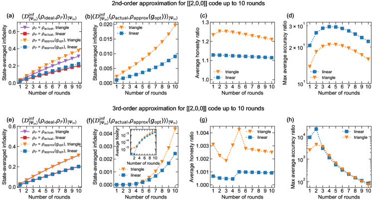
Figure 7: Results simulated by using the second-order $\hat{\mathcal{N}}_{\mathrm{approx},2}(g_{\mathrm{opt}})$ [upper panels: (a), (b), (c), and (d)] and third-order $\hat{\mathcal{N}}_{\mathrm{approx},3}(g_{\mathrm{opt}})$ [lower panels: (e), (f), (g), and (h)] approximate noise channels, where $g_{\mathrm{opt}}$ is the optimal gain factor chosen to maximize the approximation accuracy subject to the honesty criterion [Eq. (12)]. The values of $g_{\mathrm{opt}}$ for the second-order approximate noise channels are $g_{\mathrm{opt}}\simeq 1.14$ for linear and $g_{\mathrm{opt}}\simeq 1.2$ for triangle geometry. For the third-order approximation, $g_{\mathrm{opt}}\simeq 1.0005$ for linear and $g_{\mathrm{opt}}\simeq 1.002$ for triangle geometry. Panels (a,b,e,f): State-averaged infidelity between the data-qubits density matrices simulated by using (a,e) ideal and actual noise channels (solid lines), ideal and approximate noise channels (dotted lines), (b,f) actual and approximate noise channels (Inset of panel f: Semilog plot). Panels (c,d,g,h): (c,g) state-averaged honesty ratio calculated using $g_{\mathrm{opt}}$, (d,h) maximum state-averaged accuracy ratio calculated using $g_{\mathrm{opt}}$.

Based on the simulations of the infidelities at each round of the $\llbracket 2,0,0\rrbracket$ code, we plot the state-averaged results for the second-order and third-order approximate noise channels as a function of round number in the upper and lower panels of Fig. 7, respectively. The approximate density matrices $\rho_{\mathrm{approx}}$ are calculated using the optimal gain factor ($g_{\mathrm{opt}}$) [Eq. (11)], which makes the approximate channels honest and as accurate as possible. Here we show the results for both linear and triangular connectivities.

Panels (a), (b), (e) and (f) of Fig. 7 show the state-averaged infidelities of the data-qubits density matrices calculated after each round of the $\llbracket 2,0,0\rrbracket$ code, where the averaging is performed over the four different input Bell states. In Figs. 7(a) and 7(e), the infidelities between the data-qubits density matrices of the ideal ($\rho_{\mathrm{ideal}}$) and actual ($\rho_{\mathrm{actual}}$) channels are plotted using solid lines, while the infidelities between the data-qubits density matrices of the ideal ($\rho_{\mathrm{ideal}}$) and approximate ($\rho_{\mathrm{approx}}$) channels are depicted by dashed lines. Figures 7(b) and  7(f) show the infidelities between the data-qubits density matrices of the actual ($\rho_{\mathrm{actual}}$) and approximate ($\rho_{\mathrm{approx}}$) channels. These infidelities increase with the number of rounds because the noise decoherence effect accumulates as the number of rounds increases, which in turn increases the distance between the density matrices. The increase is larger for the triangle geometry compared to the linear connectivity because the triangle geometry has one more extra crosstalk channel due to the coupling between qubits 1 and 2 (see Fig. 4).

The state-averaged honesty ratios for the approximate channels are plotted in panels (c) and (g) of Fig. 7. The results are calculated using the optimal gain factor ($g_{\mathrm{opt}}$) which is the gain factor that maximizes the state-averaged accuracy ratios subject to the constraint that the approximate channel must be honest (i.e., honesty ratio $\geq 1$ [Eq. (12)]) for all four Bell input states. Using this optimal gain factor $g_{\mathrm{opt}}$, we compute the state-averaged accuracy ratios, which are shown in panels (d) and (h) of Fig. 7. As seen in Figs. 7(d) and 7(h), the accuracy of the approximation first increases with the number of rounds and for a large enough round number ($>$ 5 for the second-order and $>$ 3 for the third-order approximation), the accuracy decreases with the number of rounds due to the accumulation of the noise decoherence effect. The reason for the nonmonotonic behavior of the accuracy ratio as a function of round number is because the distance between $\rho_{\mathrm{ideal}}$ and $\rho_{\mathrm{actual}}$ increases roughly linearly with the number of rounds [Figs. 7(a) and 7(e)] while the distance between $\rho_{\mathrm{actual}}$ and $\rho_{\mathrm{approx}}$ grows exponentially with the number of rounds [Figs. 7(b) and 7(f)]. Note that in going from the second-order to the third-order approximation, the accuracy ratio increases by $\sim 1-2$ orders of magnitude, which implies that the three-body correlated noise has significant effects on the actual performance of the code.

VI Conclusions and Outlook

We propose a generic perturbative series approach, based on the cluster-expansion method, for decomposing the Lindbladian noise in a Markovian channel into components based on the qubit-qubit correlation degrees. Furthermore, we also present a systematic way to construct honest and accurate approximate noise channels from the decomposed Lindbladians, where the accuracy (efficiency) increases (decreases) as we include correlated noise components with higher and higher correlation degrees. Our work provides a general technique to characterize correlated errors,which goes beyond the Pauli noise model [21, 22] and also the commonly assumed approximate noise acting on only one or two qubits.

By applying the cluster expansion approach to a concrete physical setting, namely, fixed-frequency superconducting qubits coupled via static always-on interactions, we show that for realistic parameter sets common to this setup, correlated noise beyond two qubits have significant effects on the performance of QEC. While here we focus on superconducting qubits, our technique can actually be applied to any kind of quantum computing platform. Moreover, our method can be extended to more complex settings, such as multi-level qubit systems, where effects due to noncomputational states (e.g., leakage) can be taken into account, and also to larger number of qubits. Crucially, our technique gives systematic characterization of the correlated-noise components of higher and higher degrees as the system size increases. This systematic order-by-order noise characterization allows us to quantify the smallest maximum degree of noise correlation that needs to be taken into account for a certain desired accuracy in the noise modeling of large quantum processors. Our approach therefore paves the way towards constructing an accurate, honest and scalable approximate simulation of large quantum devices.

Appendix A Superoperator representation

Quantum channels are completely positive and trace preserving (CPTP) linear maps that act on a $d\times d$ density matrices $\rho=\sum_{i,j=1}^{d}\rho_{ij}|e_{i}\rangle\langle e_{j}|$. We can represent quantum channels and their generators (i.e., the Lindbladian for our case here) in the superoperator representation where they become $d^{2}\times d^{2}$ matrices acting on a vectorized $d^{2}\times 1$ density operator $|\rho\rangle\rangle=\sum_{i,j=1}^{d}\rho_{ij}|e_{i}\rangle\otimes|e_{j}\rangle$. Operators that act on the bra and ket now transform into operators acting on different copies of the Hilbert space $\mathcal{H}\otimes\mathcal{H}$, i.e., $\hat{A}\rho\hat{B}\rightarrow\hat{A}\otimes\hat{B}^{T}|\rho\rangle\rangle$, where the superscript $T$ indicates a matrix transpose. As a result, in the superoperator representation, the Lindblad master equation [Eq.(2)] is written as $\partial_{t}|\rho(t)\rangle\rangle=\hat{\mathcal{L}}|\rho(t)\rangle\rangle$, where we use the symbol $\;\hat{}\;$ to denote the superoperator representation, e.g., $\mathcal{L}\rightarrow\hat{\mathcal{L}}$.

Using the superoperator representation, we write the Lindbladian as

$$\hat{\mathcal{L}} =-i(\hat{H}\otimes\mathds{1}-\mathds{1}\otimes\hat{H}^{T})$$

$$\hskip 14.22636pt+\sum_{j}\gamma_{j}\left(\hat{A}_{j}\otimes\hat{A}_{j}^{*}-\frac{1}{2}\hat{A}_{j}^{\dagger}\hat{A}_{j}\otimes\mathds{1}-\frac{1}{2}\mathds{1}\otimes\hat{A}_{j}^{T}\hat{A}_{j}^{*}\right).$$ (23)

As a result, the action of a superoperator on a density matrix becomes simply a matrix-vector multiplication. Furthermore, the composition of superoperators is given by a product of the matrix representations of the superoperators. In the superoperator representation, a quantum channel is therefore given by the matrix exponentiation of its Lindbladian generator, i.e., $\hat{\mathcal{V}}=\hat{T}\left[\exp(\int_{0}^{t}\hat{\mathcal{L}}(t^{\prime})dt^{\prime})\right]$. At any given time $t$, the state of the system is then given by $|\rho(t)\rangle\rangle=\hat{\mathcal{V}}|\rho(0)\rangle\rangle$.

Appendix B Example applications of the cluster expansion approach

In this Appendix, we give two examples of the application of our cluster expansion method. As the first example, we consider the simplest case, i.e., a Lindbladian of a three-qubit quantum processor which consists of only a jump operator acting on qubit 1:

$$\hat{\widetilde{\mathcal{L}}}=\hat{\Lambda}^{\{1\}},$$ (24)

where $\Lambda^{\{1\}}(\rho)=\gamma_{1}\left(\hat{A}_{1}\rho\hat{A}_{1}^{\dagger}-\frac{1}{2}\hat{A}_{1}^{\dagger}\hat{A}_{1}\rho-\frac{1}{2}\rho\hat{A}_{1}^{\dagger}\hat{A}_{1}\right)$ contains only the jump operator $\hat{A}_{1}$ acting on qubit 1. Using the cluster expansion in Eq. (III), we have the decomposed Lindbladian as

$$\hat{\widetilde{\mathcal{L}}}^{\{1\}} =\mathrm{ln}\left(\mathrm{Tr}_{23}\left[e^{\hat{\Lambda}^{\{1\}}}\left(\mathds{1}_{\{1\}}\otimes\frac{\mathds{1}_{\{2,3\}}}{4}\right)\right]\otimes\mathds{1}_{\{2,3\}}\right)$$

$$=\hat{\Lambda}^{\{1\}},$$ (25a)

$$\hat{\widetilde{\mathcal{L}}}^{\{2\}} =\mathrm{ln}\left(\mathrm{Tr}_{13}\left[e^{\hat{\Lambda}^{\{1\}}}\left(\mathds{1}_{\{2\}}\otimes\frac{\mathds{1}_{\{1,3\}}}{4}\right)\right]\otimes\mathds{1}_{\{1,3\}}\right)$$

$$=0,$$ (25b)

$$\hat{\widetilde{\mathcal{L}}}^{\{3\}} =\mathrm{ln}\left(\mathrm{Tr}_{12}\left[e^{\hat{\Lambda}^{\{1\}}}\left(\mathds{1}_{\{3\}}\otimes\frac{\mathds{1}_{\{1,2\}}}{4}\right)\right]\otimes\mathds{1}_{\{1,2\}}\right)$$

$$=0,$$ (25c)

$$\hat{\widetilde{\mathcal{L}}}^{\{1,2\}} =\mathrm{ln}\left(\mathrm{Tr}_{3}\left[e^{\hat{\Lambda}^{\{1\}}}\left(\mathds{1}_{\{1,2\}}\otimes\frac{\mathds{1}_{\{3\}}}{2}\right)\right]\otimes\mathds{1}_{\{3\}}\right)$$

$$\hskip 14.22636pt-\hat{\widetilde{\mathcal{L}}}^{\{1\}}-\hat{\widetilde{\mathcal{L}}}^{\{2\}}$$

$$=0,$$ (25d)

$$\hat{\widetilde{\mathcal{L}}}^{\{1,3\}} =\mathrm{ln}\left(\mathrm{Tr}_{2}\left[e^{\hat{\Lambda}^{\{1\}}}\left(\mathds{1}_{\{1,3\}}\otimes\frac{\mathds{1}_{\{2\}}}{2}\right)\right]\otimes\mathds{1}_{\{2\}}\right)$$

$$\hskip 14.22636pt-\hat{\widetilde{\mathcal{L}}}^{\{1\}}-\hat{\widetilde{\mathcal{L}}}^{\{3\}}$$

$$=0,$$ (25e)

$$\hat{\widetilde{\mathcal{L}}}^{\{2,3\}} =\mathrm{ln}\left(\mathrm{Tr}_{1}\left[e^{\hat{\Lambda}^{\{1\}}}\left(\mathds{1}_{\{2,3\}}\otimes\frac{\mathds{1}_{\{1\}}}{2}\right)\right]\otimes\mathds{1}_{\{1\}}\right)$$

$$\hskip 14.22636pt-\hat{\widetilde{\mathcal{L}}}^{\{2\}}-\hat{\widetilde{\mathcal{L}}}^{\{3\}}$$

$$=0,$$ (25f)

$$\hat{\widetilde{\mathcal{L}}}^{\{1,2,3\}} =\hat{\widetilde{\mathcal{L}}}-\hat{\widetilde{\mathcal{L}}}^{\{1\}}-\hat{\widetilde{\mathcal{L}}}^{\{2\}}-\hat{\widetilde{\mathcal{L}}}^{\{3\}}$$

$$\hskip 14.22636pt-\hat{\widetilde{\mathcal{L}}}^{\{1,2\}}-\hat{\widetilde{\mathcal{L}}}^{\{2,3\}}-\hat{\widetilde{\mathcal{L}}}^{\{1,3\}}$$

$$=0.$$ (25g)

As expected, the cluster expansion gives only a non-trivial Lindbladian acting on qubit 1. In evaluating Eq. (25), we have used the fact that $\mathrm{Tr}\left[e^{\hat{\Lambda}^{\{1\}}}\rho\right]=1$, since $e^{\hat{\Lambda}^{\{1\}}}$ is a CPTP map which preserves the trace of density matrices.

As a second example, let us consider the Lindbladian of a three-qubit quantum processor which comprises a jump operator acting on both qubits 1 and 2, i.e.,

$$\hat{\widetilde{\mathcal{L}}}=\hat{\Lambda}^{\{1,2\}},$$ (26)

where

$$\Lambda^{\{1,2\}}(\rho)=\gamma_{1,2}\left(\hat{A}_{1,2}\rho\hat{A}_{1,2}^{\dagger}-\frac{1}{2}\hat{A}_{1,2}^{\dagger}\hat{A}_{1,2}\rho-\frac{1}{2}\rho\hat{A}_{1,2}^{\dagger}\hat{A}_{1,2}\right)$$ (27)

consists of a correlated jump operator $\hat{A}_{1,2}$ acting on both qubits 1 and 2. We decompose the Lindbladian using the cluster expansion [Eq. (III)] as

$$\hat{\widetilde{\mathcal{L}}}^{\{1\}} =\mathrm{ln}\left(\mathrm{Tr}_{23}\left[e^{\hat{\Lambda}^{\{1,2\}}}\left(\mathds{1}_{\{1\}}\otimes\frac{\mathds{1}_{\{2,3\}}}{4}\right)\right]\otimes\mathds{1}_{\{2,3\}}\right)$$

$$=\mathrm{ln}\left(\mathrm{Tr}_{2}\left[\frac{1}{2}e^{\hat{\Lambda}^{\{1,2\}}}\right]\right)\equiv\langle\hat{\Lambda}^{\{1,2\}}\rangle_{2},$$ (28a)

$$\hat{\widetilde{\mathcal{L}}}^{\{2\}} =\mathrm{ln}\left(\mathrm{Tr}_{13}\left[e^{\hat{\Lambda}^{\{1,2\}}}\left(\mathds{1}_{\{2\}}\otimes\frac{\mathds{1}_{\{1,3\}}}{4}\right)\right]\otimes\mathds{1}_{\{1,3\}}\right)$$

$$=\mathrm{ln}\left(\mathrm{Tr}_{1}\left[\frac{1}{2}e^{\hat{\Lambda}^{\{1,2\}}}\right]\right)\equiv\langle\hat{\Lambda}^{\{1,2\}}\rangle_{1},$$ (28b)

$$\hat{\widetilde{\mathcal{L}}}^{\{1,2\}} =\hat{\Lambda}^{\{1,2\}}-\langle\hat{\Lambda}^{\{1,2\}}\rangle_{2}-\langle\hat{\Lambda}^{\{1,2\}}\rangle_{1},$$ (28c)

$$\hat{\widetilde{\mathcal{L}}}^{\{3\}} =\hat{\widetilde{\mathcal{L}}}^{\{2,3\}}=\hat{\widetilde{\mathcal{L}}}^{\{1,3\}}=\hat{\widetilde{\mathcal{L}}}^{\{1,2,3\}}=0.$$ (28d)

The total Lindbladian is therefore decomposed into components that act on qubit 1, qubit 2 and both qubits 1 and 2. The single-qubit components $\hat{\widetilde{\mathcal{L}}}^{S_{1}}$ (e.g., $\hat{\widetilde{\mathcal{L}}}^{\{1\}},\hat{\widetilde{\mathcal{L}}}^{\{2\}}$) of the Lindbladian can be thought of as parts of the Lindbladian that act on each qubit irrespective of the other qubits states, and the two-qubit components $\hat{\widetilde{\mathcal{L}}}^{S_{2}}$ (e.g., $\hat{\widetilde{\mathcal{L}}}^{\{1,2\}}$) of the Lindbladian describe pure two-qubit correlations. Note that while the single-qubit components $\hat{\widetilde{\mathcal{L}}}^{S_{1}}$ of the Lindbladian obtained from the cluster expansion approach are guaranteed to be a physical Lindbladian, the higher-order correlated components $\hat{\widetilde{\mathcal{L}}}^{S_{m>1}}$ are not guaranteed to be physical. However, in this work we find that we can construct a CPTP approximate noise channel by choosing appropriate gain factors for each of the Lindbladian components in Eq. (11).

Appendix C Simulation results for the triangle geometry

In this Appendix, we present results calculated for the 8th round of the $\llbracket 2,0,0\rrbracket$ code in the triangle geometry. Figure 8 shows the infidelities between different quantum channels where the approximate channels are simulated using the second- and third-order approximations. The overall qualitative behaviors of the results for the triangle geometry are similar to those of the linear geometry shown in Fig. 6 of Sec. V.

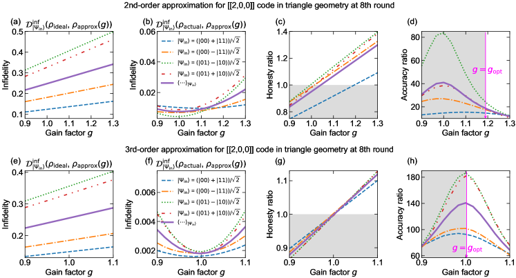
Figure 8: Results simulated for the triangular connectivity using the second-order $\hat{\mathcal{N}}_{\mathrm{approx},2}$ [upper panels: (a), (b), (c) and (d)] and third-order $\hat{\mathcal{N}}_{\mathrm{approx},3}$ [lower panels: (e), (f), (g) and (h)] approximate noise channels. They are calculated at the 8th round implementation of the $\llbracket 2,0,0\rrbracket$ code for different input data-qubits states $|\Psi_{\mathrm{in}}\rangle$; the state-averaged results are denoted by $\langle\cdots\rangle_{|\Psi_{\mathrm{in}}\rangle}$ and shown as solid purple lines. (a,b,e,f) Infidelity between the data-qubits density matrices as a function of gain factor $g$: (a,e) Infidelity between ideal and approximate density matrices, (b,f) Infidelity between actual and approximate density matrices. (c,g) Honesty ratio as a function of gain factor $g$. (d,h) Accuracy ratio as a function of gain factor $g$. Magenta arrow denotes $g=g_{\mathrm{opt}}$, i.e., the optimal value of $g$ that maximizes the state-averaged accuracy ratio subject to the honesty criterion [Eq. (12)], where $g_{\mathrm{opt}}\simeq 1.2$ for the second-order and $g_{\mathrm{opt}}\simeq 1.002$ for the third-order approximate channel. Shaded areas in panels (c), (d), (g), and (h) denote regimes where approximate noise models are not honest (honesty ratio $<1$).

References

- Shor [1995] P. W. Shor, Scheme for reducing decoherence in quantum computer memory, Phys. Rev. A 52, R2493 (1995).
- Shor [1996] P. W. Shor, Fault-tolerant quantum computation, in Proceedings of 37th conference on foundations of computer science (IEEE, 1996) p. 56.
- Calderbank and Shor [1996] A. R. Calderbank and P. W. Shor, Good quantum error-correcting codes exist, Phys. Rev. A 54, 1098 (1996).
- Devitt et al. [2013] S. J. Devitt, W. J. Munro, and K. Nemoto, Quantum error correction for beginners, Reports on Progress in Physics 76, 076001 (2013).
- Aharonov and Ben-Or [1997] D. Aharonov and M. Ben-Or, Fault-tolerant quantum computation with constant error, in Proceedings of the twenty-ninth annual ACM symposium on Theory of computing (1997) p. 176.
- Gottesman [1998] D. Gottesman, Theory of fault-tolerant quantum computation, Phys. Rev. A 57, 127 (1998).
- Preskill [1998] J. Preskill, Reliable quantum computers, Proceedings of the Royal Society of London. Series A: Mathematical, Physical and Engineering Sciences 454, 385 (1998).
- Knill et al. [1998] E. Knill, R. Laflamme, and W. H. Zurek, Resilient quantum computation, Science 279, 342 (1998).
- Guillaud and Mirrahimi [2019] J. Guillaud and M. Mirrahimi, Repetition cat qubits for fault-tolerant quantum computation, Phys. Rev. X 9, 041053 (2019).
- Darmawan et al. [2021] A. S. Darmawan, B. J. Brown, A. L. Grimsmo, D. K. Tuckett, and S. Puri, Practical quantum error correction with the xzzx code and kerr-cat qubits, PRX Quantum 2, 030345 (2021).
- Chamberland et al. [2022] C. Chamberland, K. Noh, P. Arrangoiz-Arriola, E. T. Campbell, C. T. Hann, J. Iverson, H. Putterman, T. C. Bohdanowicz, S. T. Flammia, A. Keller, G. Refael, J. Preskill, L. Jiang, A. H. Safavi-Naeini, O. Painter, and F. G. Brandão, Building a fault-tolerant quantum computer using concatenated cat codes, PRX Quantum 3, 010329 (2022).
- Bonilla Ataides et al. [2021] J. P. Bonilla Ataides, D. K. Tuckett, S. D. Bartlett, S. T. Flammia, and B. J. Brown, The xzzx surface code, Nature communications 12, 2172 (2021).
- Blume-Kohout et al. [2017] R. Blume-Kohout, J. K. Gamble, E. Nielsen, K. Rudinger, J. Mizrahi, K. Fortier, and P. Maunz, Demonstration of qubit operations below a rigorous fault tolerance threshold with gate set tomography, Nature communications 8, 14485 (2017).
- Nielsen et al. [2021] E. Nielsen, J. K. Gamble, K. Rudinger, T. Scholten, K. Young, and R. Blume-Kohout, Gate set tomography, Quantum 5, 557 (2021).
- Proctor et al. [2020] T. Proctor, M. Revelle, E. Nielsen, K. Rudinger, D. Lobser, P. Maunz, R. Blume-Kohout, and K. Young, Detecting and tracking drift in quantum information processors, Nature communications 11, 5396 (2020).
- Paris and Rehacek [2004] M. Paris and J. Rehacek, Quantum state estimation, Vol. 649 (Springer Science & Business Media, 2004).
- Howard et al. [2006] M. Howard, J. Twamley, C. Wittmann, T. Gaebel, F. Jelezko, and J. Wrachtrup, Quantum process tomography and linblad estimation of a solid-state qubit, New Journal of Physics 8, 33 (2006).
- Samach et al. [2022] G. O. Samach, A. Greene, J. Borregaard, M. Christandl, J. Barreto, D. K. Kim, C. M. McNally, A. Melville, B. M. Niedzielski, Y. Sung, D. Rosenberg, M. E. Schwartz, J. L. Yoder, T. P. Orlando, J. I.-J. Wang, S. Gustavsson, M. Kjaergaard, and W. D. Oliver, Lindblad tomography of a superconducting quantum processor, Phys. Rev. Appl. 18, 064056 (2022).
- Emerson et al. [2005] J. Emerson, R. Alicki, and K. Życzkowski, Scalable noise estimation with random unitary operators, Journal of Optics B: Quantum and Semiclassical Optics 7, S347 (2005).
- Magesan et al. [2011] E. Magesan, J. M. Gambetta, and J. Emerson, Scalable and robust randomized benchmarking of quantum processes, Phys. Rev. Lett. 106, 180504 (2011).
- Harper et al. [2020] R. Harper, S. T. Flammia, and J. J. Wallman, Efficient learning of quantum noise, Nature Physics 16, 1184 (2020).
- Van Den Berg et al. [2023] E. Van Den Berg, Z. K. Minev, A. Kandala, and K. Temme, Probabilistic error cancellation with sparse pauli–lindblad models on noisy quantum processors, Nature Physics 19, 1116 (2023).
- Harper and Flammia [2023] R. Harper and S. T. Flammia, Learning correlated noise in a 39-qubit quantum processor, PRX Quantum 4, 040311 (2023).
- Emerson et al. [2007] J. Emerson, M. Silva, O. Moussa, C. Ryan, M. Laforest, J. Baugh, D. G. Cory, and R. Laflamme, Symmetrized characterization of noisy quantum processes, Science 317, 1893 (2007).
- Silva et al. [2008] M. Silva, E. Magesan, D. W. Kribs, and J. Emerson, Scalable protocol for identification of correctable codes, Phys. Rev. A 78, 012347 (2008).
- Onorati et al. [2021] E. Onorati, T. Kohler, and T. Cubitt, Fitting quantum noise models to tomography data, arXiv:2103.17243 (2021).
- Onorati et al. [2023] E. Onorati, T. Kohler, and T. S. Cubitt, Fitting time-dependent markovian dynamics to noisy quantum channels, arXiv:2303.08936 (2023).
- Lindblad [1976] G. Lindblad, On the generators of quantum dynamical semigroups, Communications in Mathematical Physics 48, 119 (1976).
- Gorini et al. [1976] V. Gorini, A. Kossakowski, and E. C. G. Sudarshan, Completely positive dynamical semigroups of n-level systems, Journal of Mathematical Physics 17, 821 (1976).
-
Note [1]
We remark that, given the target , there exists a family
of such forms
for with . In addition, summation over a function also produces appropriate forms, e.g., with the only requirement to ensure that is the identity channel when there is no noise. There can be circumstances where use of such forms may be desirable, due to averaging or simplification for the appropriate setting, but here we fix as the normal form.(29) - Mayer and Montroll [1941] J. E. Mayer and E. Montroll, Molecular distribution, The Journal of Chemical Physics 9, 2 (1941).
- Kira and Koch [2011] M. Kira and S. W. Koch, Semiconductor quantum optics (Cambridge University Press, 2011).
- Note [2] While the term in Eq. (III) is not guaranteed to be a physical Lindbladian, the first term of the right-hand side of Eq. (III), i.e., , is always a physical Lindbladian as it describes noise in an -qubits subsystem.
- Note [3] In general, one may have to use different gain factors for different decomposed components of the Lindbladian to get a completely-positive and trace-preserving (CPTP) approximate noise channel that is honest and accurate. However, for our case of code in 3-qubit processors, we find that we can use the same gain factor for all the Lindbladian components to obtain honest and accurate CPTP approximate noise channels.
- Magesan et al. [2013] E. Magesan, D. Puzzuoli, C. E. Granade, and D. G. Cory, Modeling quantum noise for efficient testing of fault-tolerant circuits, Phys. Rev. A 87, 012324 (2013).
- Puzzuoli et al. [2014] D. Puzzuoli, C. Granade, H. Haas, B. Criger, E. Magesan, and D. G. Cory, Tractable simulation of error correction with honest approximations to realistic fault models, Phys. Rev. A 89, 022306 (2014).
- Gutiérrez and Brown [2015] M. Gutiérrez and K. R. Brown, Comparison of a quantum error-correction threshold for exact and approximate errors, Phys. Rev. A 91, 022335 (2015).
- Jozsa [1994] R. Jozsa, Fidelity for mixed quantum states, Journal of modern optics 41, 2315 (1994).
- Nielsen and Chuang [2010] M. A. Nielsen and I. L. Chuang, Quantum computation and quantum information (Cambridge university press, 2010).
- Rigetti and Devoret [2010] C. Rigetti and M. Devoret, Fully microwave-tunable universal gates in superconducting qubits with linear couplings and fixed transition frequencies, Phys. Rev. B 81, 134507 (2010).
- Chow et al. [2011] J. M. Chow, A. D. Córcoles, J. M. Gambetta, C. Rigetti, B. R. Johnson, J. A. Smolin, J. R. Rozen, G. A. Keefe, M. B. Rothwell, M. B. Ketchen, and M. Steffen, Simple all-microwave entangling gate for fixed-frequency superconducting qubits, Phys. Rev. Lett. 107, 080502 (2011).
- Sheldon et al. [2016] S. Sheldon, E. Magesan, J. M. Chow, and J. M. Gambetta, Procedure for systematically tuning up cross-talk in the cross-resonance gate, Phys. Rev. A 93, 060302 (2016).
- Johansson et al. [2012] J. R. Johansson, P. D. Nation, and F. Nori, Qutip: An open-source python framework for the dynamics of open quantum systems, Computer Physics Communications 183, 1760 (2012).
- Johansson et al. [2013] J. Johansson, P. Nation, and F. Nori, Qutip 2: A python framework for the dynamics of open quantum systems, Computer Physics Communications 184, 1234 (2013).