Chirality-induced emergent spin-orbit coupling in topological atomic lattices

Abstract

Spin-orbit coupled dynamics are of fundamental interest in both quantum optical and condensed matter systems alike. In this work, we show that photonic excitations in pseudospin-1/2 atomic lattices exhibit an emergent spin-orbit coupling when the geometry is chiral. This spin-orbit coupling arises naturally from the electric dipole interaction between the lattice sites and leads to spin polarized excitation transport. Using a general quantum optical model, we determine analytically the conditions that give rise to spin-orbit coupling and characterize the behavior under various symmetry transformations. We show that chirality-induced spin textures are associated with a topologically nontrivial Zak phase that characterizes the chiral setup. Our results demonstrate that chiral atom arrays are a robust platform for realizing spin-orbit coupled topological states of matter.

I Introduction

The spin-orbit (SO) interaction refers to the coupling of a particle’s intrinsic angular momentum to its motional degrees of freedom. For an electron moving in an electrostatic potential, this phenomenon can be interpreted as arising from a Lorentz transformation of the electric field in the laboratory frame to a momentum dependent magnetic field that couples directly to the electron’s spin in its rest frame. The resulting spin-momentum locking and associated spin textures can result in nontrivial topological properties [1, 2] and are of considerable interest in the development of new spintronics devices [3, 4, 5]. In particular, the generation of long-lived nonequilibrium spin currents is crucial for designing efficient spin transistors, spin diodes, and other related technologies [6].

Recently, various photonic and quantum optical systems have emerged as attractive candidates for realizing SO coupled dynamics. Those involving photonic nanostructures have demonstrated the SO coupling of photons using the circular polarizations of light [7, 8, 9, 10]. In cold atoms, pairs of internal hyperfine states can act as pseudospin-1/2 systems that resemble electronic spin degrees of freedom [11]. Coupling these states to coherent laser fields can produce synthetic SO potentials in ultracold Fermi gases [12, 13, 14] and Bose-Einstein condensates [15]. In addition to ultracold gases comprised of moving atoms, the hyperfine levels of atoms or atom-like emitters arranged in ordered lattices can also be used as pseudospin-1/2 states. Such atomic arrays support the transport of optical excitations in a manner analogous to electrons in traditional crystal lattices [16, 17, 18] and can be leveraged as quantum simulation platforms to study spin dependent transport processes in a highly tunable environment.

In a related Letter, we demonstrate that the collective Bloch modes of pseudospin-1/2 atomic arrays experience an emergent SO coupling when the lattice geometry is chiral [19]. In this case, the associated photonic band structure exhibits a finite spin texture and a topologically nontrivial Zak phase. In turn, these spin bands result in spin dependent dynamics which manifest as polarization selective photon transport and superradiant emission. In this work, we present a general description of the emergent SO coupling and topological properties associated with chiral atomic lattices. Our findings are distinct from those of previous works in that, here, the SO coupling results from the phase dependence of the electric dipole field that arises naturally from the chirality of the geometry itself. We determine the analytical conditions that give rise to SO coupling in propagating optical excitations and characterize the behavior under different symmetry transformations. Our results demonstrate that chiral atom arrays are a robust platform for realizing SO coupled topological states of matter.

II Theoretical Formalism

In order to study SO coupled transport, we consider ordered arrays of dipole-coupled quantum emitters (e.g., atoms, molecules, quantum dots) at fixed positions within the laboratory frame. The pseudospin degree of freedom for each emitter, $i$, is encoded in a V-type level structure consisting of a single ground state, $\ket{g_{i}}$, and two hyperfine states, $\ket{\uparrow_{i}}$ and $\ket{\downarrow_{i}}$, corresponding to the two orthogonal polarizations of circularly polarized light [Fig. 1(a)]. The bare hyperfine states are assumed to have identical resonance frequencies, $\omega_{0}=2\pi c/\lambda_{0}$, where $\lambda_{0}$ is the wavelength of each optical transition and $c$ is speed of light in vacuum.

II.1 Dipole-dipole interactions

The transport of optical excitations between quantum emitters in free space involves long-range interactions mediated by a radiation field. It is convenient to trace out the field degrees of freedom in the Born and Markov approximations to obtain an effective descriptive in terms of the matter operators only [20, 21]. In free space, the effective interactions between quantum electric dipoles at points $\mathbf{r}_{i}$ and $\mathbf{r}_{j}$ are determined by the dyadic Green’s tensor

$$\mathbf{G}(\mathbf{r}_{ij},\omega_{0})=\frac{e^{ik_{0}r_{ij}}}{4\pi k_{0}^{2}r_{ij}^{3}}\Big{[}(k_{0}^{2}r_{ij}^{2}+ik_{0}r_{ij}-1)\openone\\ -(k_{0}^{2}r_{ij}^{2}+3ik_{0}r_{ij}-3)\frac{\mathbf{r}_{ij}\otimes\mathbf{r}_{ij}}{r_{ij}^{2}}\Big{]},$$ (1)

where $\mathbf{r}_{ij}=\mathbf{r}_{i}-\mathbf{r}_{j}$, $r_{ij}=\lvert\mathbf{r}_{ij}\rvert$, and $k_{0}=\omega_{0}/c$ (see also Appendix A). The coherent and dissipative parts of the dipole-dipole interaction are then given by

$$J^{\sigma\sigma^{\prime}}_{ij} =-\frac{3}{2}\lambda_{0}\Gamma_{0}\boldsymbol{\varepsilon}^{\dagger}_{i\sigma}\cdot\operatorname{Re}\mathbf{G}(\mathbf{r}_{ij},\omega_{0})\cdot\boldsymbol{\varepsilon}_{j\sigma^{\prime}}$$ (2)

$$\Gamma^{\sigma\sigma^{\prime}}_{ij} =3\lambda_{0}\Gamma_{0}\boldsymbol{\varepsilon}^{\dagger}_{i\sigma}\cdot\operatorname{Im}\mathbf{G}(\mathbf{r}_{ij},\omega_{0})\cdot\boldsymbol{\varepsilon}_{j\sigma^{\prime}},$$ (3)

where $\boldsymbol{\varepsilon}_{i\sigma}$ is the circular polarization vector for orbital $\sigma\in\{\uparrow,\downarrow\}$ on emitter $i$, $\Gamma_{0}\equiv\Gamma_{ii}^{\sigma\sigma}=\omega_{0}^{3}\lvert\boldsymbol{\wp}_{i\sigma}\rvert^{2}/(3\pi\hbar\epsilon_{0}c^{3})$ is the spontaneous emission rate associated with each excited state orbital, $\boldsymbol{\wp}_{i\sigma}$ is the transition dipole matrix element vector, and $\epsilon_{0}$ is the vacuum permittivity. The interactions therefore depend only on the scalar distance between the emitters and on the relative orientations of the polarization vectors. These polarization vectors are defined with respect to a quantization axis, $\hat{\mathbf{q}}$, about which the optically excited orbitals are circularly polarized. The orientation of the quantization axis relative to the symmetry planes of the lattice is directly related to the emergence of SO coupling in chiral systems (Section III). For general $\hat{\mathbf{q}}$, the polarization vectors for left and right circularly polarized excitations are given by

$$\boldsymbol{\varepsilon}_{\uparrow\downarrow}=\frac{1}{\sqrt{2}}(\hat{\mathbf{d}}_{1}\pm i\hat{\mathbf{d}}_{2}),$$ (4)

where $\uparrow$ ($\downarrow$) corresponds to $+$ ($-$), $\hat{\mathbf{d}}_{1}$ and $\hat{\mathbf{d}}_{2}$ denote the orthonormal vectors defining the polarization plane, and $\hat{\mathbf{d}}_{1}\times\hat{\mathbf{d}}_{2}=\hat{\mathbf{q}}$.

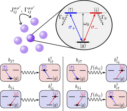
FIG. 1: (a) Schematic of the V-type level structure considered in this work. The excited state orbitals have resonant frequency $\omega_{0}$ and spontaneous emission rate $\Gamma_{0}$. Emitters are coupled with coherent and dissipative hopping rates $J_{ij}^{\sigma\sigma^{\prime}}$ and $\Gamma_{ij}^{\sigma\sigma^{\prime}}$, respectively. (b) Interactions between emitters $i$ and $j$ are mediated through photon exchanges that excite orbitals with either the same (left) or opposite (right) polarization. When the photon spin is changed, conservation of angular momentum requires that the interaction picks up an additional position-dependent phase.

II.2 Open system dynamics

The unitary dynamics for an arbitrary arrangement of V-type quantum emitters interacting via the Greeen’s tensor formalism are generated by the Hamiltonian

$$H=\sum_{i=1}^{N}\sum_{\sigma}\omega_{0}\ket{\sigma_{i}}\bra{\sigma_{i}}+\sum^{N}_{i,j\neq i=1}\sum_{\sigma,\sigma^{\prime}}J_{ij}^{\sigma\sigma^{\prime}}\ket{\sigma_{i}}\bra{\sigma^{\prime}_{j}}$$ (5)

(we set $\hbar\equiv 1$ here and throughout). The non-unitary contributions of collective dissipation and single emitter spontaneous emission are included via the Lindbladian

$$\mathcal{L}[\rho]=\sum^{N}_{i,j=1}\frac{\Gamma_{ij}^{\sigma\sigma^{\prime}}}{2}\left(2\ket{g}\bra{\sigma^{\prime}_{j}}\rho\ket{\sigma_{i}}\bra{g}-\left\{\ket{\sigma_{i}}\bra{\sigma^{\prime}_{j}},\rho\right\}\right).$$ (6)

Here, $\ket{g}$ denotes the collective ground state of the multi-atom system, and we assume that thermal effects are negligible. The full open system dynamics for the state $\rho(t)$ are then given by the quantum optical master equation $\dot{\rho}=-i[H,\rho]+\mathcal{L}[\rho]$.

Throughout this work, we focus on the single-excitation subspace which is sufficient to observe SO coupled transport. For single-excitation states, the master equation dynamics are equivalent to those evoked by the non-Hermitian effective Hamiltonian

$$H_{\mathrm{eff}}=\sum_{i=1}^{N}\sum_{\sigma}\omega_{0}b^{{\dagger}}_{i\sigma}b_{i\sigma}-\frac{3}{2}\lambda_{0}\Gamma_{0}\sum^{N}_{i,j\neq i=1}\sum_{\sigma,\sigma^{\prime}}G_{ij}^{\sigma\sigma^{\prime}}b^{{\dagger}}_{i\sigma}b_{j\sigma^{\prime}},$$ (7)

where $b^{{\dagger}}_{i\sigma}$ ($b_{i\sigma}$) denotes a bosonic creation (annihilation) operator satisfying $[b_{i\sigma},b^{{\dagger}}_{i\sigma}]=1$, and $G_{ij}^{\sigma\sigma^{\prime}}=\boldsymbol{\varepsilon}^{\dagger}_{i\sigma}\cdot\mathbf{G}(\mathbf{r}_{ij},\omega_{0})\cdot\boldsymbol{\varepsilon}_{j\sigma^{\prime}}$. We may further trace over the ground state of each emitter and denote the excited states using the basis vector mapping $\ket{\uparrow}=\begin{pmatrix}1&0\end{pmatrix}^{T}$, $\ket{\downarrow}=\begin{pmatrix}0&1\end{pmatrix}^{T}$ such that the circularly polarized excitations at each emitter site behave as pseudospin-1/2 degrees of freedom characterized by the $2\times 2$ Pauli matrices. The operator $b^{\dagger}_{\uparrow}b_{\uparrow}-b^{\dagger}_{\downarrow}b_{\downarrow}=\ket{\uparrow}\bra{\uparrow}-\ket{\downarrow}\bra{\downarrow}=\sigma_{z}$ then quantifies the relative spin population in each emitter.

Finally, it is useful to define a set of collective operators that act on the spin indices of each emitter simultaneously. We denote

$$\mathcal{S}_{\alpha}\equiv\openone\otimes\sigma_{\alpha}$$ (8)

for $\alpha\in\{x,y,z\}$, where $\openone$ is the identity matrix acting on the spatial indices. The pseudospin operator for a delocalized state extending across multiple emitters then follows simply as $\mathcal{S}_{z}$.

II.3 Photonic band structures

In order to characterize the spin properties of pseudospin-1/2 atomic lattices, we will assess the photonic band structures obtained by transforming the real space Hamiltonian into momentum space. For simplicity, we limit the discussion to lattices that are periodic only along one direction. In this case, the site index for a non-Bravais lattice composed of $\mathcal{N}$ sublattices can be decomposed into $i=(m,\mu)$ where $m\in[1,M]$ indexes the unit cell along the axis of periodicity and $\mu\in[1,\mathcal{N}]$ denotes the sublattice index. In the limit of large $M$, the substitution $b_{i\sigma}=(1/\sqrt{M})\sum_{\mathbf{{k}}}\exp{(i\mathbf{{k}}\cdot\mathbf{r}_{m\mu})}b_{\mathbf{{k}}\mu\sigma}$ for quasimomentum $\mathbf{{k}}$ yields $H_{\mathrm{eff}}=\sum_{\mathbf{{k}}}H(\mathbf{{k}})$, where the Bloch Hamiltonian

$$H(\mathbf{{k}})=\sum_{\mu,\nu}\sum_{\sigma,\sigma^{\prime}}h_{\mu\sigma,\nu\sigma^{\prime}}(\mathbf{{k}})b^{{\dagger}}_{\mathbf{{k}}\mu\sigma}b_{\mathbf{{k}}\nu\sigma^{\prime}}$$ (9)

has matrix elements [17, 18]

$$h_{\mu\sigma,\nu\sigma^{\prime}}(\mathbf{{k}})=\omega_{0}\delta_{\mu\nu}\delta_{\sigma\sigma^{\prime}}+\chi^{I}_{\mu\sigma,\nu\sigma^{\prime}}+\chi^{II}_{\mu\sigma,\nu\sigma^{\prime}}$$ (10)

for

$$\chi^{I}_{\mu\sigma,\nu\sigma^{\prime}} =-\frac{3}{2}\lambda_{0}\Gamma_{0}\sum_{\mathbf{R}_{\mu}\neq 0}e^{-i\mathbf{{k}}\cdot\mathbf{R}_{\mu}}G_{\sigma\sigma^{\prime}}(\mathbf{R}_{\mu})\delta_{\mu\nu}$$ (11)

$$\chi^{II}_{\mu\sigma,\nu\sigma^{\prime}} =-\frac{3}{2}\lambda_{0}\Gamma_{0}\sum_{\mathbf{R}_{\mu}}e^{-i\mathbf{{k}}\cdot\mathbf{R}_{\mu}}G_{\sigma\sigma^{\prime}}(\mathbf{R}_{\mu}+\mathbf{n}_{\mu\nu})(1-\delta_{\mu\nu})$$ (12)

(see also Appendix B). Here, the (infinite) set of $\mathbf{R}_{\mu}$ denotes vectors of the underlying Bravais lattice and $\mathbf{n}_{\mu\nu}=\mathbf{n}_{\mu}-\mathbf{n}_{\nu}$ is the basis vector pointing from sublattice $\nu$ to $\mu$ within a given unit cell. The off-diagonal terms $\chi^{I}$ and $\chi^{II}$ describe interactions between emitters on the same and different sublattices, respectively. Like the real-space Hamiltonian, it is important to note that $H(\mathbf{{k}})$ is, in general, non-Hermitian.

III Conditions for Spin-Orbit Coupling

The emergence of SO coupling and finite spin polarizations within pseudospin-1/2 atomic lattices require a nontrivial spin texture for the Bloch modes. Put differently, the spin $\braket{\mathcal{S}_{z}}$ must be nonzero at some point in the Brillouin zone in order to observe SO coupling and spin dependent transport. As a main result, we now determine analytically the conditions for $\braket{\mathcal{S}_{z}}\neq 0$. In particular, we will show that SO coupling emerges in systems that lack inversion symmetry about axes in the polarization plane, which motivates a generalized definition of chirality for pseudospin-1/2 bosons.

Quite generally, the spin of each Bloch mode is constrained to be zero if there exists a symmetry of the Bloch Hamiltonian that reverses the spin of each mode for all $\mathbf{{k}}$. We can write this symmetry as $W\equiv\mathcal{S}_{x}V$, where

$$V\ket{\mathbf{R},\mu,\sigma}=\sum_{\nu}\hat{V}_{\mu\nu}\ket{\mathbf{R},\nu,\sigma}$$ (13)

and $\hat{V}$ is a $2\mathcal{N}\times 2\mathcal{N}$ unitary matrix acting on the sublattice indices. Note that $V$ preserves the sign of $\mathbf{R}$. In other words, $W$ is an operator that reverses the spin but leaves the lattice geometry—including the Bravais lattice vectors—invariant, up to a unitary transformation of the sublattice indices.

To see that this symmetry prohibits spinful Bloch bands, consider a general Bloch Hamiltonian $H(\mathbf{{k}})$ with orthonormal eigenstates $\ket{u_{n}(\mathbf{{k}})}$ and corresponding eigenvalues $\varepsilon_{n}(\mathbf{{k}})$. We do not require $H(\mathbf{{k}})$ to be Hermitian or time reversal ($\mathcal{T}$) invariant (see Section IV.2). By construction, $[H(\mathbf{{k}}),W]=0$ such that

$$WH(\mathbf{{k}})\ket{u_{n}(\mathbf{{k}})}=H(\mathbf{{k}})W\ket{u_{n}(\mathbf{{k}})}=\varepsilon_{n}(\mathbf{{k}})W\ket{u_{n}(\mathbf{{k}})}.$$ (14)

The states $\ket{u_{n}(\mathbf{{k}})}$ and $\ket{u_{m}(\mathbf{{k}})}\equiv W\ket{u_{n}(\mathbf{{k}})}$ are therefore both eigenstates of $H(\mathbf{{k}})$ with the same eigenvalue . Noting that $[V,\mathcal{S}_{z}]=0$ and $\mathcal{S}_{x}^{\dagger}\mathcal{S}_{z}\mathcal{S}_{x}=-\mathcal{S}_{z}$, the spins of these Bloch states satisfy

$$\braket{u_{m}(\mathbf{{k}})}{\mathcal{S}_{z}}{u_{m}(\mathbf{{k}})} =\braket{u_{n}(\mathbf{{k}})}{W^{\dagger}\mathcal{S}_{z}W}{u_{n}(\mathbf{{k}})}$$

$$=\braket{u_{n}(\mathbf{{k}})}{V^{\dagger}\mathcal{S}_{x}^{\dagger}\mathcal{S}_{z}\mathcal{S}_{x}V}{u_{n}(\mathbf{{k}})}$$

$$=-\braket{u_{n}(\mathbf{{k}})}{\mathcal{S}_{z}}{u_{n}(\mathbf{{k}})}.$$ (15)

Now, by orthonormality, we must have $\braket{u_{m}(\mathbf{{k}})}{u_{n}(\mathbf{{k}})}=\delta_{mn}$. If $\braket{u_{m}(\mathbf{{k}})}{u_{n}(\mathbf{{k}})}=1$, then there is no degeneracy and $\ket{u_{m}(\mathbf{{k}})}=e^{i\phi(\mathbf{{k}})}\ket{u_{n}(\mathbf{{k}})}$ for $\phi(\mathbf{{k}})\in\mathbb{R}$. That is, $\ket{u_{m}(\mathbf{{k}})}$ and $\ket{u_{n}(\mathbf{{k}})}$ represent the same state up to a $U(1)$ gauge ambiguity. In this case, it follows trivially from Eq. (III) that $\braket{\mathcal{S}_{z}}=0$. If, on the other hand, $\braket{u_{m}(\mathbf{{k}})}{u_{n}(\mathbf{{k}})}=0$, then the states are orthogonal with equal and opposite spin (see, e.g., the $\mathcal{N}=1$ case of Fig. 4 in Ref. [19]). However, because the states are degenerate, the linear combinations $\ket{u_{\pm}(\mathbf{{k}})}\equiv(1/\sqrt{2})(\ket{u_{n}(\mathbf{{k}})}\pm\ket{u_{m}(\mathbf{{k}})})$ are also eigenstates of $H(\mathbf{{k}})$ with the same eigenvalue. These superposition states satisfy $\braket{\mathcal{S}_{z}}=0$ by construction. It follows that if $W$ is a symmetry of the Bloch Hamiltonian, then one may always construct a basis such that all Bloch modes have zero spin.

The remaining task is to relate this result back to the geometrical properties of the system. If the lattice contains an inversion center at position $\mathbf{R}=0$, then the parity ($\mathcal{P}$) operator may be written as [23],

$$\mathcal{P}\ket{\mathbf{R},\mu,\sigma}=\sum_{\nu}\hat{\mathcal{P}}_{\mu\nu}\ket{-\mathbf{R},\mu,\sigma}.$$ (16)

That is, $\mathcal{P}$ acts by inverting the spatial coordinates of the unit cell, up to a unitary transformation on the sublattice indices. We require that $\mathcal{P}$ leave the spin indices invariant because angular momentum is an axial vector. In this case, the Bloch bands are inversion symmetric about $\mathbf{{k}}=0$, and the Bloch Hamiltonian satisfies $\mathcal{P}H(\mathbf{{k}})\mathcal{P}^{-1}=H(-\mathbf{{k}})$. Analogously, we may write

$$W\ket{\mathbf{R},\mu,\sigma}=\sum_{\nu}\hat{V}_{\mu\nu}\ket{\mathbf{R},\nu,\bar{\sigma}},$$ (17)

where $\ket{\bar{\sigma}}=\sigma_{x}\ket{\sigma}$ denotes the opposite spin state. The operator $W$ therefore acts as a “spin inversion” (as opposed to spatial inversion) while preserving the real space coordinates of the unit cell. Heuristically, $\mathcal{P}$ acts to negate the sign of the lattice vectors, $\mathbf{R}$ (or equivalently the quasimomentum, $\mathbf{{k}}$), whereas $W$ negates the sign of the quantization axis, $\mathbf{q}$. Thus, for $W$ to be a symmetry of the Bloch Hamiltonian, there must exist a unitary transformation that relates the original and spin-flipped configurations while preserving the mutual orientation of the basis vectors together with $\mathbf{{k}}$ and $\mathbf{q}$. If such a transformation does not exist, then the spin inversion symmetry of the combined lattice-quantization axis system is broken. We may therefore take this as the definition of chirality for pseudospin-1/2 bosonic systems. In the following section, we will demonstrate how this generalized definition of chirality has a straightforward interpretation in terms of orthogonal transformations of the real space lattice geometry.

IV Symmetry Analysis of Spin Bands

IV.1 Orthogonal group symmetries

In order to study how the condition for nontrivial spin textures relates back to the geometry of the system, we now consider transformations under representations of the orthogonal group $O(3)$. Each unit cell associated with Bravais lattice vector $\mathbf{R}$ contains $2\mathcal{N}$ states labeled by $\ket{\mathbf{R},n}$, where $n=(\mu,\sigma)$ is a composite index denoting the subblatice and spin. If the unit cell is invariant under an orthogonal transformation $U$, then the operator corresponding to this symmetry may be written as

$$U\ket{\mathbf{R},n}=\sum_{m}\hat{U}_{nm}\ket{U\mathbf{R},m},$$ (18)

where $\hat{U}$ is a $2\mathcal{N}\times 2\mathcal{N}$ unitary matrix. Indeed, the parity operator (16) is one such operator. The particular form of $\hat{U}_{nm}$ depends on the symmetry operation in question and on the structure of the unit cell. Nevertheless, a number of general relations can be deduced that apply to all Hamiltonians of the form (7).

We are particularly interested in transformations that satisfy Eq. (17) for spin inversion symmetry. The simplest case occurs for lattices that possess a mirror plane. In this case, the basis vectors $\mathbf{n}_{\mu}$ exist in mirror-symmetric pairs such that $\mathbf{n}_{\nu}=\mathcal{R}_{M}\mathbf{n}_{\mu}$ for reflection operator $\mathcal{R}_{M}$ (note also that $\mu=\nu$ when the lattice vectors $\mathbf{R}_{\mu}$ lie in the mirror plane). If this mirror plane also contains the quantization axis, then the corresponding operator $\mathcal{R}_{\mathbf{q},M}$ acts on the basis states as

$$\mathcal{R}_{\mathbf{q},M}\ket{\mathbf{R},\mu,\sigma}=\ket{\mathcal{R}_{\mathbf{q},M}\mathbf{R},\nu,\bar{\sigma}}.$$ (19)

This transformation satisfies Eq. (17), provided $\mathcal{R}_{\mathbf{q},M}\mathbf{R}=\mathbf{R}$. That is, if the lattice possesses a mirror plane that contains the quantization axis and the Bravais lattice vectors, then the spin of each Bloch mode is guaranteed to be zero.

The transformation (19) is not the only form of $W$ that imposes trivial spin textures. Rotoreflections are also possible, so long as the combined operation satisfies Eq. (17). To flip the spin, the rotation should be by an angle $\pi$ about an axis lying in the polarization plane. Denoting this rotation as $R_{\perp}(\pi)$, the transformation

$$R_{\perp}(\pi)\mathcal{R}_{\mathbf{q}}\ket{\mathbf{R},\mu,\sigma}=\ket{R_{\perp}(\pi)\mathcal{R}_{\mathbf{q}}\mathbf{R},\nu,\bar{\sigma}}$$ (20)

also fulfills Eq. (17) but for a broader class of lattice geometries that satisfy $R_{\perp}(\pi)\mathcal{R}_{\mathbf{q}}\mathbf{R}=\mathbf{R}$ and $R_{\perp}(\pi)\mathcal{R}_{\mathbf{q}}\mathbf{n}_{\mu}=\mathbf{n}_{\nu}$. The physical interpretation of this result is that the Bloch modes have zero spin when the polarization plane contains a symmetry axis of improper rotation.

The considerations above justify the notion of spin inversion symmetry breaking as a form of generalized chirality for pseudospin-1/2 systems. Whereas true chirality is usually defined as a lack of any axis of improper rotation, here we only require that such an axis not lie in the polarization plane. The latter definition naturally encompasses the former, but also includes additional configurations where the chirality stems from the mutual orientation of the lattice vectors and the quantization axis, rather than from the lattice geometry alone (Section VI).

IV.2 Time-reversal symmetry

In addition to the geometry of the system, the behavior under time-reversal also influences the spin properties of the system. The dipole-dipole interaction present in Eq. (5) describes the creation (destruction) of an excitation at site $i$ ($j$) with a rate determined by the Green’s tensor (1). This process neglects electronic exchange interactions, which is a good approximation when the spacing between adjacent emitters is much larger than the spatial extent of the atomic wavefunctions. In this case, the circularly polarized excitations at each emitter site can be described using bosonic statistics and with a bosonic time-reversal operator. Generally, a Hamiltonian $H$ is $\mathcal{T}$-invariant if and only if there exists a unitary operator $U_{\mathcal{T}}$ such that $\mathcal{T}H\mathcal{T}^{-1}=H$ for $\mathcal{T}=\mathcal{K}U_{\mathcal{T}}$, where $\mathcal{K}$ is the anti-unitary complex conjugation operator $\mathcal{K}:i\to-i$ [24]. For Hamiltonians of the form (5), the time-reversal operator is given by

$$\mathcal{T}=\mathcal{K}\mathcal{S}_{x}$$ (21)

and satisfies $\mathcal{T}^{2}=1$. This represents an important distinction from traditional electronic systems and significantly influences the spin textures of the resulting photonic bands.

In traditional band theory, spin-1/2 electrons obeying fermionic statistics exist as degenerate Kramers’ pairs when $\mathcal{T}$ symmetry is preserved. If inversion symmetry is also present, this constraint requires at least a two-fold degeneracy at every point in the Brillouin zone. If inversion symmetry is broken, $\mathcal{T}$ invariance still requires this degeneracy be preserved at all $\mathcal{T}$ invariant quasimomenta. In either case, the spin of each excitation may be interpreted as a vector on the Bloch sphere.

In bosonic bands, no such degeneracy is required. For the pseudospins described by Eq. (4), the polarization of each excitation is instead given by a vector on the Poincare sphere [25, 26] with left and right circular polarizations residing at the north and south poles, respectively. In contrast to the fermionic case (where an equal superposition of $\uparrow$ and $\downarrow$ spins results in an equal magnitude spin-1/2 excitation pointing in the orthogonal plane), vectors residing along the equator of the Poincare sphere do not carry angular momentum. That is, an equal superposition of left and right circularly polarized excitations yields a linearly polarized excitation of pseudospin-0 [see Eq. (4)]. Whereas the $\mathcal{T}$ operator acting on a fermionic system corresponds to a complete inversion of the Bloch vector through the origin, the bosonic $\mathcal{T}$ results in a reflection through the Poincare sphere equatorial plane and leaves vectors residing in this plane unchanged.

In later sections, we will consider the influence of broken $\mathcal{T}$ symmetry as induced by the anti-Hermitian part of the effective Hamiltonian (7). To this end, it is instructive to present a more detailed description of the considerations above. In particular, direct application of Eq. (21) demonstrates that the pseudospin operator is time-odd, obeying $\mathcal{T}\mathcal{S}_{z}\mathcal{T}^{-1}=-\mathcal{S}_{z}$. If the Hamiltonian is time-reversal invariant, then $[H,\mathcal{T}]=0$ and

$$\mathcal{T}H\mathcal{T}^{-1}=\mathcal{K}\mathcal{S}_{x}H(\mathcal{K}\mathcal{S}_{x})^{-1}=\mathcal{S}_{x}H^{*}\mathcal{S}^{-1}_{x}=H.$$ (22)

A general Bloch Hamiltonian $H(\mathbf{{k}})=e^{-i\mathbf{{k}}\cdot\mathbf{r}}He^{i\mathbf{{k}}\cdot\mathbf{r}}$ then satisfies

$$\mathcal{T}H(\mathbf{{k}})\mathcal{T}^{-1}=e^{i\mathbf{{k}}\cdot\mathbf{r}}\mathcal{S}_{x}H^{*}\mathcal{S}^{-1}_{x}e^{-i\mathbf{{k}}\cdot\mathbf{r}}=H(-\mathbf{{k}}),$$ (23)

where $H(-\mathbf{{k}})=\mathcal{S}_{x}H^{*}(\mathbf{{k}})\mathcal{S}^{-1}_{x}$. The Brillouin zone contains a set of time-reversal invariant momenta, $\mathbf{{k}}=\Gamma^{i}$, where $-\Gamma^{i}=\Gamma^{i}+\mathbf{G}_{\mu}$ and $\mathbf{G}_{\mu}$ is a reciprocal lattice vector, $\mathbf{G}_{\mu}\cdot\mathbf{R}_{\mu}=2\pi$ (to avoid ambiguity with other quantities denoted by $\Gamma$, we will always use a superscript to denote time-reversal invariant momenta). At these points, the Bloch Hamiltonian satisfies $[H(\Gamma^{i}),\mathcal{T}]=0$. To see how the bosonic $\mathcal{T}$ influences the degeneracy of the resulting Bloch bands, consider $\ket{u_{n}(\mathbf{{k}})}$ as a general eigenstate of $H(\mathbf{{k}})$ with eigenvalue $\varepsilon_{n}(\mathbf{{k}})$. As in the previous section, the spin associated with this state is given by $\braket{\mathcal{S}_{z}}$. Away from the $\Gamma^{i}$ points, the spin of this state is, in general, nonzero (Section III). Applying Eq. (23), the Bloch Hamiltonian for a time-reversal invariant system satisfies

$$\mathcal{T}H(\mathbf{{k}})\ket{u_{n}(\mathbf{{k}})}=H(-\mathbf{{k}})\mathcal{T}\ket{u_{n}(\mathbf{{k}})}=\varepsilon_{n}(\mathbf{{k}})\mathcal{T}\ket{u_{n}(\mathbf{{k}})}$$ (24)

such that $\ket{u_{m}(-\mathbf{{k}})}\equiv\mathcal{T}\ket{u_{n}(\mathbf{{k}})}$ is an eigenstate of $H(-\mathbf{{k}})$ with the same energy, $\varepsilon_{m}(-\mathbf{{k}})=\varepsilon_{n}(\mathbf{{k}})$. The states at $\mathbf{{k}}$ and $-\mathbf{{k}}$ necessarily have opposite spin:

$$\braket{u_{m}(-\mathbf{{k}})}{\mathcal{S}_{z}}{u_{m}(-\mathbf{{k}})} =\braket{u_{n}(\mathbf{{k}})}{\mathcal{T}^{\dagger}\mathcal{S}_{z}\mathcal{T}}{u_{n}(\mathbf{{k}})}$$

$$=\braket{u^{*}_{n}(\mathbf{{k}})}{\mathcal{S}_{x}\mathcal{S}_{z}\mathcal{S}_{x}^{-1}}{u^{*}_{n}(\mathbf{{k}})}$$

$$=-\braket{u_{n}(\mathbf{{k}})}{\mathcal{S}_{z}}{u_{n}(\mathbf{{k}})},$$ (25)

where the second step follows from $\mathcal{S}_{x}=\mathcal{S}_{x}^{\dagger}=\mathcal{S}_{x}^{-1}$ and the third step from the Hermiticity of $\mathcal{S}_{z}$. However, because $\mathcal{T}^{2}=1$, $\ket{u_{m}(\mathbf{{k}})}$ and $\ket{u_{n}(\mathbf{{k}})}$ need not represent orthogonal states. In the absence of accidental degeneracies, these states are instead equal (up to a phase) such that each band $n$ is symmetric about $\Gamma^{i}$ in energy and antisymmetric in spin. The requirement at $\mathbf{{k}}=\Gamma^{i}$ then follows simply as

$$\braket{u_{n}(\Gamma^{i})}{\mathcal{S}_{z}}{u_{n}(\Gamma^{i})}=-\braket{u_{n}(\Gamma^{i})}{\mathcal{S}_{z}}{u_{n}(\Gamma^{i})}=0$$ (26)

for each band individually, and no two-fold spin degeneracy is required.

In position space, the eigenstates are equal superpositions of states at $\mathbf{{k}}$ and $-\mathbf{{k}}$. The antisymmetric spin textures required by $\mathcal{T}$ invariance therefore dictate that all position space eigenstates have zero spin. However, this does not preclude the emergence of nontrivial spin textures, which requires only that the spin be nonzero at a single point in the Brillouin zone. If this point has nonzero dispersion, then the antisymmetric nature of the spin bands—together with the symmetric nature of the energy bands—implies spin-momentum locking for all $\mathcal{T}$-invariant systems with nonzero spin. If $\mathcal{T}$ symmetry is broken, this antisymmetric condition need not apply, and the position space eigenstates may also exhibit nonzero spin (Section V).

Finally, it should be noted that we have defined $V$ explicitly as a unitary operator. However under certain conditions, the symmetry $[H(\mathbf{{k}}),W]=0$ may be satisfied by an anti-unitary operator, $W=\mathcal{S}_{x}\tilde{V}$. In this case,

$$WH(\mathbf{{k}})W^{-1}=V\mathcal{S}_{x}H^{*}(\mathbf{{k}})\mathcal{S}_{x}^{-1}V^{-1}=V\mathcal{T}H(\mathbf{{k}})\mathcal{T}^{-1}V^{-1},$$ (27)

and SO coupling can only emerge by breaking $\mathcal{T}$-invariance. In analogy with Barron [27], we denote systems obeying $[H(\mathbf{{k}}),W]\neq 0$ for both unitary and anti-unitary $W$ as “truly chiral,” and those for which this condition holds only for unitary $W$ as “falsely chiral.”

IV.3 Inversion and anti-inversion symmetries

When the Hamiltonian is parity invariant, the Bloch bands are fully symmetric about $\mathbf{{k}}=\Gamma^{i}$. Similarly, when the Hamiltonian is time-reversal invariant, the Bloch bands are symmetric in energy and antisymmetric in spin. Suppose now that the Hamiltonian is invariant not under $\mathcal{P}$ or $\mathcal{T}$ but under the unitary operator

$$\bar{\mathcal{P}}\ket{\mathbf{R},\mu,\sigma}=\sum_{\nu}\hat{\mathcal{P}}_{\mu\nu}\ket{-\mathbf{R},\mu,\bar{\sigma}}.$$ (28)

The matrix representation $\hat{\bar{\mathcal{P}}}=\hat{\mathcal{P}}\otimes\sigma_{x}$ then acts as the parity operator but treats the spin degree of freedom as a polar vector that is odd under inversion (for a 1D lattice, we may also interpret this operation as a series of rotations). Consequently, $[H,\bar{\mathcal{P}}]=0$ implies $\bar{\mathcal{P}}H(\mathbf{{k}})\bar{\mathcal{P}}^{-1}=H(-\mathbf{{k}})$ such that

$$\bar{\mathcal{P}}H(\mathbf{{k}})\ket{u_{n}(\mathbf{{k}})}=H(-\mathbf{{k}})\bar{\mathcal{P}}\ket{u_{n}(\mathbf{{k}})}=\varepsilon_{n}(\mathbf{{k}})\bar{\mathcal{P}}\ket{u_{n}(\mathbf{{k}})}.$$ (29)

In analogy with Eqs. (24) and (IV.2), the states $\ket{u_{n}(\mathbf{{k}})}$ and $\bar{\mathcal{P}}\ket{u_{n}(\mathbf{{k}})}$ have equal energy and opposite spin on opposite sides of the Brillouin zone. The operator $\bar{\mathcal{P}}$ therefore acts as a sort of “anti-inversion” by enforcing a spin antisymmetry about $\mathbf{{k}}=\Gamma^{i}$. Importantly, this symmetry is a property of the lattice geometry and the orientation of the quantization axis, and is independent of the behavior under $\mathcal{T}$.

V Chiral lattices

We are now in a position to study specific lattice geometries. We first consider “chiral lattices,” which we define as those exhibiting either true or false chirality for all orientations of $\mathbf{q}$. The quintessential chiral structure is a right circular helix, which serves as a paradigmatic example. This structure is periodic along its longitudinal helical axis which, without loss of generality, we choose to be parallel to the $z$-axis (Fig. 2). The lattice vectors of the underlying Bravais lattice are then given by $\mathbf{R}_{\mu}=al\hat{\mathbf{z}}$ for lattice constant $a$ and $l\in\mathbb{Z}$. For a right-handed helix periodic along the $z$-axis with radius $r_{0}$, pitch $a$, and $\mathcal{N}$ emitters per unit cell, the emitter positions are given by

$$\mathbf{r}_{j}=r_{0}\cos(\phi_{j})\hat{\mathbf{x}}+r_{0}\sin(\phi_{j})\hat{\mathbf{y}}+\frac{a\phi_{j}}{2\pi}\hat{\mathbf{z}},$$ (30)

where $\phi_{j}=2\pi(j-1)/\mathcal{N}$. The relative coordinate between emitters $i$ and $j$ can then be written as $\mathbf{r}_{ij}=x_{ij}\hat{\mathbf{x}}+y_{ij}\hat{\mathbf{y}}+z_{ij}\hat{\mathbf{z}}$ for

$$x_{ij} =-2r_{0}\sin\left[(\mu-\nu)\frac{\pi}{\mathcal{N}}\right]\sin\left[(\mu+\nu)\frac{\pi}{\mathcal{N}}\right]$$

$$y_{ij} =2r_{0}\sin\left[(\mu-\nu)\frac{\pi}{\mathcal{N}}\right]\cos\left[(\mu+\nu)\frac{\pi}{\mathcal{N}}\right]$$

$$z_{ij} =\left[(\mu-\nu)\frac{a}{\mathcal{N}}+al\right].$$ (31)

Here, $\mu\ (\nu)=i\ (j)\ \mathrm{mod}\ \mathcal{N}+1$ for integers $i,j\in[1,N]$ and $l$ denotes the number of unit cells between $i$ and $j$ (i.e., $l=0$ if $i$ and $j$ are in the same unit cell). We note that with this choice of coordinates, the $\mu=1$ sublattice lies on the positive $x$-axis.

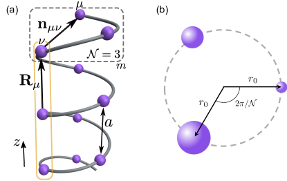
FIG. 2: (a) Schematic of the helical lattice geometry for pitch $a$ and $\mathcal{N}=3$. The dashed grey rectangle denotes one unit cell, whereas the solid yellow rectangle denotes one sublattice. (b) Top-down view of the helical lattice. The sublattices are arranged with radial position $r_{0}$ and azimuthal separation $2\pi/\mathcal{N}$.

V.1 Longitudinal circular polarization

As a demonstration of true chirality, we first orient the quantization axis to lie along the axis of periodicity ($\hat{\mathbf{q}}=\hat{\mathbf{z}}$). In this case, $r_{0}=\varrho_{i}=\varrho_{j}$ and the spin-flip interaction is found to be

$$G_{ij}^{\uparrow\downarrow}=\frac{3r_{0}^{2}\lambda_{0}\Gamma_{0}}{4\pi k_{0}^{2}r_{ij}^{5}}\sin^{2}\left(\frac{\phi_{i}-\phi_{j}}{2}\right)e^{-i(\phi_{i}+\phi_{j})}\\ \times e^{ik_{0}r_{ij}}\left(3-k_{0}^{2}r_{ij}^{2}-i3k_{0}r_{ij}\right),$$ (32)

where $\phi_{i}=\tan^{-1}(y_{i}/x_{i})$. A reflection through the $y$-$z$ plane then takes $\phi_{i}\to-\phi_{i}$ such that $G_{ij}^{\uparrow\downarrow}\to G_{ij}^{\downarrow\uparrow}$ (see also Appendix C). The spin dynamics are therefore interchanged by reflections perpendicular to the polarization plane that transform the right-handed helix to its left-handed mirror image.

The photonic band structures for left- and right-handed helices are shown in Fig. 3(a). Because the helix geometry lacks an axis of improper rotation, the symmetry $[H(\mathbf{{k}}),W]\neq 0$ is broken for all unitary $W$ and the Bloch bands exhibit nontrivial spin textures. As a consequence of this broken symmetry, the longitudinally polarized helix supports bulk helical modes that mediate the spin-momentum locking of propagating wave packets. This dynamical effect is illustrated by the spin antisymmetry of the band structures. Away from the $\Gamma^{i}$ points, each Bloch mode acquires a finite group velocity $v_{n}(k)=\partial\varepsilon_{n}(k)/\partial k$ along the axis of periodicity. Because of the spin antisymmetry, these modes exhibit a helicity $\eta=\braket{\mathcal{S}_{z}}v/\lvert\braket{\mathcal{S}_{z}}v\rvert$ that is symmetric about $\Gamma^{i}$. When dissipative interactions are neglected [i.e., the Hamiltonian is of the form (5)], this spin-momentum locking is protected by time-reversal symmetry. Invariance of the group velocity under reflection through the $y$-$z$ plane then dictates that the two chiralities support equal and opposite helical modes.

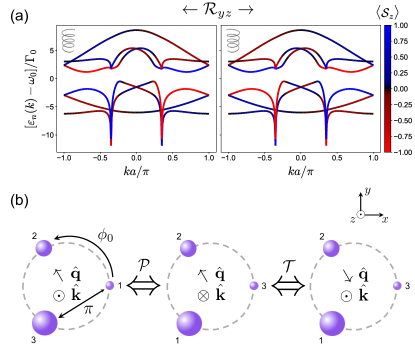
FIG. 3: (a) Band structures for the left-handed (left) and right-handed (right) helices when $\hat{\mathbf{q}}=\hat{\mathbf{z}}$. The spin bands are nontrivially antisymmetric about $\mathbf{{k}}=\Gamma^{i}$, irrespective of $\mathcal{T}$-invariance. The system exhibits true chirality with a quantized nontrivial Zak phase. Additional parameters: $\mathcal{N}=3$, $r_{0}=0.05\lambda_{0}$, $a=0.175\lambda_{0}$. (b) Top-down view of the helical unit cell for $\hat{\mathbf{q}}=\hat{\mathbf{z}}$. The $\mu=2$ sublattice serves as an anti-inversion for the lattice, and the corresponding transformation $\bar{\mathcal{P}}:(\hat{\mathbf{{k}}},\hat{\mathbf{q}})\to(-\hat{\mathbf{{k}}},-\hat{\mathbf{q}})$ enforces antisymmetric Bloch bands. If dissipation is neglected, the spin antisymmetry is also protected by $\mathcal{T}$ symmetry.

Specifically for $\hat{\mathbf{q}}=\hat{\mathbf{z}}$, the broken spin inversion symmetry persists for anti-unitary $W$ as well. Consequently, the band structures exhibit nontrivial spin textures regardless of whether the Hamiltonian is $\mathcal{T}$-invariant. When dissipative interactions are included, the Hermitian Hamiltonian (5) is replaced by the non-Hermitian effective Hamiltonian (7). In this case, $\mathcal{T}$ symmetry is broken and Eq. (IV.2) no longer holds. However, the spin antisymmetry of the Bloch bands persists because the non-Hermitian Hamiltonian remains invariant under $\bar{\mathcal{P}}$. In other words, the $z$-polarized helix contains a 1D anti-inversion center at the center of the unit cell.

To verify that the Hamiltonian is invariant under this transformation, we construct explicitly the associated matrix representation. The anti-inversion center lies at the azimuthal angle $\phi_{0}=\pi(\mathcal{N}-1)/\mathcal{N}$ (as measured from the $x$-axis) along an axis that bisects the angle between sublattices $\mu=1$ and $\mu=\mathcal{N}$. With this point chosen as the origin, the unit cell is symmetric under the combined operation of 1D spatial inversion and spin-flip. As demonstrated in Fig. 3(b), this operation is equivalent to a $\pi$ rotation about the $\phi_{0}$ axis. $\bar{\mathcal{P}}$ therefore reverses the direction of $\mathbf{q}$ and $\mathbf{{k}}$, while simultaneously exchanging the positions of the three sublattices (for odd $\mathcal{N}$, the central sublattice remains fixed). As such, the symmetry operation can be represented as $\hat{\bar{\mathcal{P}}}=X\otimes\sigma_{x}$, where $X$ is the $\mathcal{N}\times\mathcal{N}$ antidiagonal exchange matrix acting on the sublattice indices. With the above choice of origin, the basis states of each unit cell then transform as

$$\bar{\mathcal{P}}\ket{\mathbf{R},\mu,\sigma}=X\otimes\sigma_{x}\ket{-\mathbf{R},\mu,\sigma}.$$ (33)

One may verify explicitly that $[H_{\mathrm{eff}},\bar{\mathcal{P}}]=0$ and that the spin antisymmetry follows accordingly as in Eq. (29). The net result is that the longitudinally polarized helix exhibits antisymmetric spin textures that are protected by anti-inversion symmetry (or equivalently, rotational symmetry). This property manifests even in the absence of time-reversal invariance: the system is truly chiral.

To examine the topological properties of the Bloch bands, we compute the Zak phase,

$$\varphi=\oint_{\mathcal{C}}\operatorname{Tr}{[\mathbf{A}(\mathbf{{k}})]}\cdot d\mathbf{{k}}.$$ (34)

Here, $\mathbf{A}_{mn}(\mathbf{{k}})=i\braket{u_{m\mathbf{{k}}}}{\nabla_{\mathbf{{k}}}u_{n\mathbf{{k}}}}$ is the non-Abelian Berry connection matrix evaluated over a closed loop $\mathcal{C}$ around the first Brillouin zone (see Appendix D). The Zak phase is defined modulo $2\pi$ and is quantized to either $0$ (trivial) or $\pm\pi$ (topologically nontrivial) when the Hamiltonian commutes with $\mathcal{P}$ or $\bar{\mathcal{P}}$. The finite spin textures exhibited by the longitudinally polarized helix induce a nontrivial topology in the energy bands. The associated SO coupled dynamics are therefore topologically protected by the chirality of the geometry. Because of the anti-inversion center at $\phi_{0}$, the Zak phase is quantized to $\pm\pi$.

V.2 Transverse circular polarization

The symmetry properties of the non-Hermitian Hamiltonian are altered when the quantization axis is oriented perpendicular to the axis of periodicity. As an example, we consider the helix of Eq. (30) but with $\mathbf{q}$ pointing along the $\phi_{0}$ axis [Fig. 4(a)]. Because the lattice geometry is unchanged, it remains true that there is no unitary $W$ enforcing $\braket{\mathcal{S}_{z}}=0$. However, the two-fold rotational symmetry of the lattice no longer corresponds to $\bar{\mathcal{P}}$. Instead, the $\pi$ rotation that swaps the $\mu=1$ and $\mu=3$ sublattices leaves the quantization axis invariant. Consequently, the system exhibits a true inversion center and is parity symmetric with

$$\mathcal{P}\ket{\mathbf{R},\mu,\sigma}=X\otimes\openone\ket{-\mathbf{R},\mu,\sigma}.$$ (35)

The spin bands are therefore symmetric about $\mathbf{{k}}=\Gamma^{i}$ [Fig. 4(b)], and the Zak phase is quantized to $\pm\pi$.

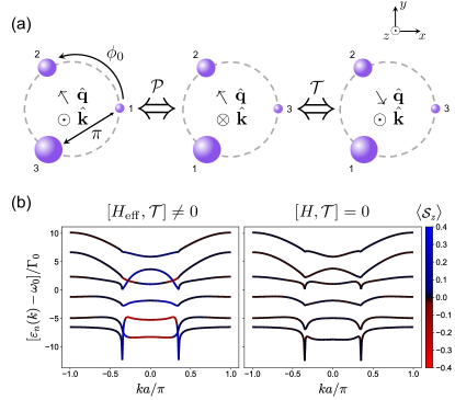
FIG. 4: (a) Top-down view of the helical unit cell for $\mathbf{q}$ oriented along the $\phi_{0}$ axis. The $\mu=1$ and $\mu=3$ sublattices are separated by an angle $\pi$ in the polarization plane such that the $\mu=2$ sublattice serves as a true inversion center. Inversion symmetry transforms $\mathcal{P}:(\hat{\mathbf{{k}}},\hat{\mathbf{q}})\to(-\hat{\mathbf{{k}}},\hat{\mathbf{q}})$, enforcing spin symmetric Bloch bands. If the Hamiltonian is also $\mathcal{T}$-invariant, the additional relation $\mathcal{T}:(\hat{\mathbf{{k}}},\hat{\mathbf{q}})\to(-\hat{\mathbf{{k}}},-\hat{\mathbf{q}})$ requires $\braket{\mathcal{S}_{z}}=0$. (b) Band structures for the $\phi_{0}$-polarized helix. The system is $\mathcal{P}$-invariant with a quantized Zak phase. When $\mathcal{T}$ symmetry is broken (left), the spin bands are symmetric about $\mathbf{{k}}=\Gamma^{i}$ and the Zak phase is topologically nontrivial. If $\mathcal{T}$ symmetry is restored (right), the combined $\mathcal{P}\mathcal{T}$ symmetry causes both the spin textures and the Zak phase to vanish. The system is therefore falsely chiral. Helix parameters are the same as in Fig. 3.

If dissipative interactions are neglected, then the Hamiltonian also commutes with $\mathcal{T}$, and the spin bands must also be antisymmetric [Eq. (IV.2)]. The combined $\mathcal{P}\mathcal{T}$ symmetry then forces $\braket{\mathcal{S}_{z}}=0$ for all $\mathbf{{k}}$ and the SO coupling is lost. In turn, the system becomes topologically trivial and the Zak phase is zero for each band. With this choice of quantization axis, the helix is only falsely chiral.

For completeness, we also present the case where $\mathbf{q}$ does not correspond to a symmetry axis of the unit cell (e.g., lies at an angle $\pi/4$ from the $x$-axis in the $x$-$y$ plane). This configuration is not invariant under $\mathcal{P}$ or $\bar{\mathcal{P}}$. Hence, when $\mathcal{T}$ symmetry is broken, the spin bands are neither symmetric nor antisymmetric (Fig. 5). If however dissipation is neglected, then the Hamiltonian is $\mathcal{T}$-invariant and the antisymmetric spin textures are restored. In either case, the Zak phase is not quantized.

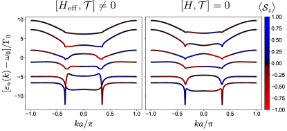
FIG. 5: Band structures for the transversely polarized helix in the absence of both $\mathcal{P}$ and $\bar{\mathcal{P}}$ invariance. When $\mathcal{T}$ symmetry is broken (left) the spin bands are neither symmetric nor antisymmetric about $\mathbf{{k}}=\Gamma^{i}$. When $\mathcal{T}$ symmetry is restored (right) the spin bands become antisymmetric. In both cases, the Zak phase is not quantized. Helix parameters are the same as in Figs. 3 and 4.

VI Chiral setups

The spin inversion symmetry breaking required for finite SO coupling need not come from the lattice geometry alone. If the lattice contains a mirror plane, there may still exist a choice of quantization axis such that the Bloch bands exhibit nontrivial spin textures. We refer to this scenario as a “chiral setup” because not all orientations of $\mathbf{q}$ satisfy $[H(\mathbf{{k}}),W]\neq 0$ for unitary $W$.

A concrete example is demonstrated by a lattice arranged into an oblique triangular prism. If the triangular faces are isosceles, then the lattice possesses a mirror plane along the axis of periodicity [Fig. 6(a)]. For simplicity, we choose the emitter positions to be circumscribed about a right circular cylinder such that $x_{ij}$ and $y_{ij}$ are given by Eq. (V), and

$$z_{ij}=\begin{cases}0,&\mu,\nu\in\{2,3\}\\ a/2,&\mu>\nu\\ -a/2,&\mu<\nu\end{cases}$$ (36)

where $\mu$ and $\nu$ are defined as before. For $\hat{\mathbf{q}}=\hat{\mathbf{x}}$, the quantization axis lies in the mirror plane [Fig. 6(b)], and the reflection operator $\mathcal{R}_{xz}$ acts as in Eq. (19). This mirror reflection commutes with both the Hermitian and non-Hermitian Hamiltonians such that the geometry is spin inversion ($W$) symmetric irrespective of the behavior under $\mathcal{T}$. It follows that $\braket{\mathcal{S}_{z}}$ must vanish for all $\mathbf{{k}}$, and the system is not chiral at all.

By contrast, if the quantization axis is instead oriented along the $y$-axis, then $\mathcal{R}_{xz}$ leaves the quantization axis invariant ($\mathbf{q}$ is an axial vector). The SO coupling is therefore preserved. Because the unit cell does not contain a center of (anti-)inversion, the Bloch bands are not fully (anti)symmetric and the Zak phase is not quantized. Nevertheless, the antisymmetry of the nontrivial spin textures is consistent with $\mathcal{T}$ symmetry, and thus the system is truly chiral.

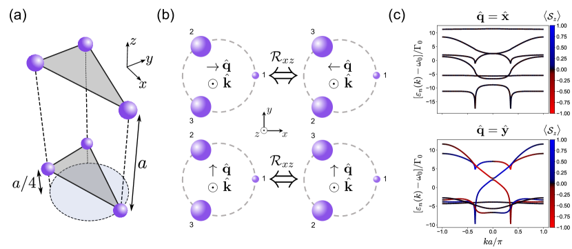
FIG. 6: (a) Lattice geometry for an oblique triangular prism. Each triangular face represents a single unit cell. The faces are assumed to be isosceles with the $x$-$z$ plane chosen as the mirror plane. (b) Top-down view of the oblique triangular prism unit cell for $\hat{\mathbf{q}}=\hat{\mathbf{x}}$ (top) and $\hat{\mathbf{q}}=\hat{\mathbf{y}}$ (bottom). (c) Band structures for the oblique triangular prism. When $\mathbf{q}$ is oriented in the mirror plane (left), the spin textures vanish irrespective of the behavior under $\mathcal{T}$. If $\mathbf{q}$ is instead oriented orthogonal to the mirror plane, then the SO coupling can be nonzero. In both cases, the Zak phase is not quantized. Additional geometrical parameters are the same as in Figs. 3, 4, and 5.

VII Spin Polarized Dynamics

Thus far, we have discussed the emergence of a finite SO coupling in pseudospin-1/2 atomic lattices based on symmetry properties alone. In order to relate these results to potential future experiments, we now demonstrate the influence of this SO coupling on the time evolution of propagating photonic excitations. The results presented in this section represent a set of testable predictions that could be verified with modern day platforms (Section VIII).

In the single excitation regime, the time dynamics of an arbitrary state $\rho(t)$ are given by the no-jump quantum master equation,

$$\dot{\rho}=-i\left(H_{\mathrm{eff}}\rho-\rho H^{\dagger}_{\mathrm{eff}}\right).$$ (37)

We consider the evolution of an initially unpolarized mixed state localized at emitter $j=1$ on the helix defined by Eq. (30). The initial state is given by

$$\rho(0)=\frac{1}{2}\left(\ket{\uparrow_{1}}\bra{\uparrow_{1}}+\ket{\downarrow_{1}}\bra{\downarrow_{1}}\right).$$ (38)

In order to quantify the magnitude of spin dependent transport, we define the spin polarization, $\Delta$, as the population difference between the $\uparrow$ and $\downarrow$ spin manifolds integrated until the wave packet reaches the opposite end of the helix at time $\tau$:

$$\Delta=\int_{0}^{\tau}dt\sum_{i}\frac{\left(\braket{b^{{\dagger}}_{i\uparrow}b_{i\uparrow}}-\braket{b^{{\dagger}}_{i\downarrow}b_{i\downarrow}}\right)}{\left(\braket{b^{{\dagger}}_{i\uparrow}b_{i\uparrow}}+\braket{b^{{\dagger}}_{i\downarrow}b_{i\downarrow}}\right)}.$$ (39)

The transport time is monitored by discretizing the helix into chunks of $N/10$ emitters, and we define $\tau$ as the time at which the total emitter population is largest in the final chunk.

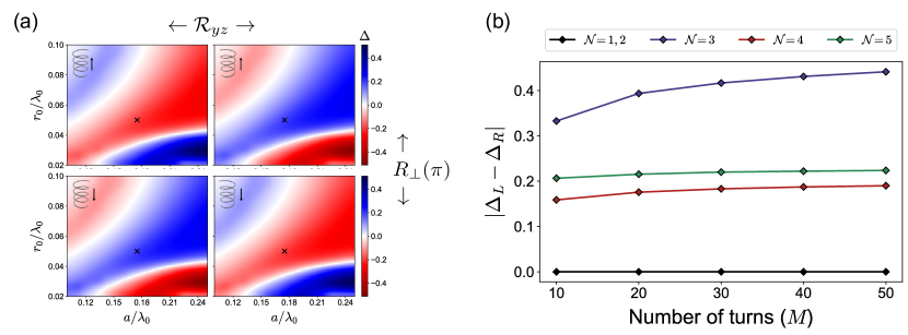
FIG. 7: (a) Spin polarization as a function of helix radius and pitch for $\hat{\mathbf{q}}=\hat{\mathbf{z}}$. Colors show the spin polarization, $\Delta$, calculated for left-handed (left) and right-handed (right) helices. A $\pi$ rotation about an axis in the polarization plane reverses the spin polarization and the direction of motion (black arrows). Black crosses denote the radius and pitch used in previous figures. Additional parameters for both panels: $\mathcal{N}=3$ emitters per $2\pi$ turn and $M=N/\mathcal{N}=20$ turns total. (b) Dependence of the spin polarization on helix length and the number of atoms per unit cell. Additional parameters: $r_{0}=0.05\lambda_{0}$, $a=0.175\lambda_{0}$, $\hat{\mathbf{q}}\cdot\hat{\mathbf{{k}}}=1$.

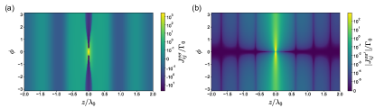
FIG. A1: Coherent coupling strengths between atoms $i$ and $j$ located on a helix with $\hat{\mathbf{q}}=\hat{\mathbf{z}}$ and radius $r_{0}=0.05\lambda_{0}$. The $x$-axis denotes the relative distance between the emitters in the $\hat{\mathbf{z}}$ direction (along the longitudinal helical axis). The $y$-axis denotes the relative azimuthal coordinate between the emitters. (a) Spin-preserving interactions. Colors denote the interaction strength $J^{\sigma\sigma}_{ij}/\Gamma_{0}$ with $\sigma\in\{\uparrow,\downarrow\}$. (b) Spin-flipping interactions. Colors denote the interaction strength $|J^{\sigma\sigma^{\prime}}_{ij}|/\Gamma_{0}$ with $\sigma,\sigma^{\prime}\in\{\uparrow,\downarrow\}$ for $\sigma\neq\sigma^{\prime}$.

Fig. 7(a) shows the value of $\Delta$ for helices with $\hat{\mathbf{q}}=\hat{\mathbf{z}}$, $\mathcal{N}=3$, and varying radius and pitch. As discussed in Section V.1, the nonzero spin polarization demonstrates the preferential transport of optical excitations with a particular helicity. Extremely large spin polarizations—upwards of 40%—are easily achievable across a wide parameter range, and we suspect that even larger spin polarizations could be achieved by further optimizing the geometry. Interestingly, for a given chirality, both the magnitude and sign of the spin polarization depend nontrivially on the geometric proportions of the helix. This fact may be traced back to the nontrivial positional dependence of the electromagnetic Green’s tensor and to the presence of long-range all-to-all couplings that introduce multiple frequency scales to the dynamics (see Fig. A1).

A reflection through the $y$-$z$ plane preserves the direction of motion but reverses the spin and transforms the left-handed lattice geometry to its right-handed mirror image. It follows from the same symmetry analysis applied to the band structures that the spin polarization is equal and opposite between the left- and right-handed geometries. If the helix is rotated by an angle $\pi$ about an axis in the polarization plane, then the chirality is preserved and both the spin polarization and the direction of motion change sign. The simultaneous reversal of the spin polarization together with the change in propagation direction demonstrates chirality dependent spin-momentum locking. Notably, for $\hat{\mathbf{q}}=\hat{\mathbf{z}}$, this $\pi$ rotation is also equivalent to a change of initial condition (38) from emitter $j=1$ to $j=N$ followed by a trivial azimuthal rotation about $\mathbf{q}$ [19].

The dependence of the spin polarization on the helix length and the number of emitters per unit cell is shown in Fig. 7(b). The $\mathcal{N}=1$ and $\mathcal{N}=2$ configurations correspond to the uniform chain and the staggered chain, respectively. These geometries are not chiral and do not exhibit any spin polarization. For the true helices ($\mathcal{N}\geq 3$), there is a modest increase in the spin polarization with increasing helix length. This trend has also been reported with electron spin polarizations in chiral molecules [28] and may be a common feature of helicity dependent transport.

VIII Towards Experimental Realizations

The results described here should be experimentally observable with readily available techniques. A standard approach would be to realize the helical geometry using neutral atoms in a 3D optical tweezer array. Coherent oscillations between atoms with V-type level structures have been demonstrated, e.g., by isolating the $60S_{1/2}$ and $60P_{3/2}$ Rydberg manifolds of ⁸⁷Rb [29, 30]. The 17.2 GHz transition frequency between these manifolds allows for subwavelength dynamics at $\mu$m-scale tweezer separations. Although the influence of dissipation may not be observable with this platform due to long Rydberg excitation lifetimes, the chirality dependent transport and topological properties of the system could still be achieved.

Dissipative dynamics could, however, be observed in a similar setup using the ${}^{3}P_{0}$ and ${}^{3}D_{1}$ manifolds of ⁸⁸Sr [31], which is commonly used in 3D optical lattice clocks [32]. Helical arrangements of atoms could be built by selectively loading particular sites of the optical lattice using an extension of the tweezer-based programmable loading scheme recently demonstrated for 2D optical lattices [33], or by employing holographic optical traps made from dielectric metasurfaces [34]. Techniques for measuring topological Bloch bands simulated with optical lattices are well-established [35, 36, 37].

An alternative setup based on a Laguerre-Gauss mode optical trapping potential may also be realized with readily available techniques [38, 39, 40]. Laguerre-Gauss modes are eigenmodes of the paraxial wave equation with orbital angular momentum quantum number, $l$. The $l=1$ mode exhibits a cylindrical geometry with a phase advance that winds once per wavelength. Interfering this mode with an orthogonally polarized plane wave shapes the field intensity into a helix. Intersecting this field with a cloud of red-detuned atoms would trap some of these atoms at intensity maxima determined by the helical potential. An additional long-range interaction potential (which could be imposed by Rydberg dressing the atoms via an additional laser [41, 42]) would result in a periodic arrangement of atoms along the helix.

Finally, the reported effects might also be observable at optical or UV wavelengths using ultra-cold chiral molecules. One option is to use artificial fluorophores conjugated to a helical molecular scaffold. Alternatively, the monomers that comprise the larger helical polymer could themselves act as individual quantum emitters and facilitate excitation transport. Such a setup could be relevant to the ongoing development of molecular spintronics devices or biomimetic light-harvesting complexes.

IX Conclusions

In this paper, we have presented a complete symmetry analysis of the SO coupling and topological properties associated with pseudospin-1/2 atomic lattices. Our results describe a general photonic excitation transport process that is unique to chiral systems and depends on the orientation of the quantization axis. These findings introduce an exciting new avenue for cold atom quantum simulators, which could be used to study the governing principles of chirality dependent photon transport in a well-controlled environment.

Because the emergence of SO coupling is dictated by the symmetries of the Bloch bands, the symmetry analysis given above is complete within the single excitation regime. Nevertheless, an interesting follow-up would be to analyze the dynamics in the multi-excitation regime. In this case, the V-type level structure imposes a hard-core boson constraint in which each atomic orbital is at most singly occupied. The ensuing non-linearity induced by the hard-core interaction is expected to result in modifications of the transport phenomena. In this regard, chiral atom arrays could serve as a promising platform for new photonics devices and for studying photonic analogues of many-body topological physics in condensed matter systems.

X Acknowledgements

The authors are grateful to Mikhail D. Lukin and Jonathan Simon for suggestions on potential experimental implementations. S.O. is supported by a postdoctoral fellowship of the Max Planck-Harvard Research Center for Quantum Optics. All authors acknowledge funding from the National Science Foundation (NSF) via the Center for Ultracold Atoms (CUA) Physics Frontiers Centers (PFC) program and via PHY-2207972, as well as from the Air Force Office of Scientific Research (AFOSR).

Appendix A The electromagnetic Green’s tensor

In free space, the effective interactions between quantum emitters are determined by the dyadic Green’s tensor, $\mathbf{G}(\mathbf{r},\mathbf{r^{\prime}},\omega)$, which is the solution to the wave equation

$$\nabla^{2}\mathbf{G}(\mathbf{r},\mathbf{r^{\prime}},\omega)-\frac{\omega^{2}}{c^{2}}\mathbf{G}(\mathbf{r},\mathbf{r^{\prime}},k)=\delta(\mathbf{r}-\mathbf{r^{\prime}})\openone$$ (40)

for observational coordinates $\mathbf{r}$, source coordinates $\mathbf{r}^{\prime}$, and frequency $\omega$. For the case where the emitters located at positions $\mathbf{r}_{j}$ are well approximated by point electric dipoles, the Green’s tensor between emitters $i$ and $j$ depends only on the relative coordinate $\mathbf{r}_{ij}=\mathbf{r}_{i}-\mathbf{r}_{j}$. In the Born and Markov approximations, the Green’s tensor may further be regarded as dispersionless and is given by [16]

$$\mathbf{G}(\mathbf{r}_{ij},\omega_{0})=\frac{e^{ik_{0}r_{ij}}}{4\pi k_{0}^{2}r_{ij}^{3}}\Big{[}(k_{0}^{2}r_{ij}^{2}+ik_{0}r_{ij}-1)\openone-(k_{0}^{2}r_{ij}^{2}+3ik_{0}r_{ij}-3)\frac{\mathbf{r}_{ij}\otimes\mathbf{r}_{ij}}{r_{ij}^{2}}\Big{]},$$ (41)

with $r_{ij}=\lvert\mathbf{r}_{ij}\rvert$ and $k_{0}=\omega_{0}/c$. The $\sigma$ component of the positive frequency electric field calculated at position $\mathbf{r}$ is then calculated (in the time domain) as [16, 43]

$$\mathbf{E}^{+}_{\sigma}(\mathbf{r})=\mu_{0}\omega_{0}^{2}\sum_{j=1}^{N}\mathbf{G}(\mathbf{r}-\mathbf{r}_{j},\omega_{0})\cdot\boldsymbol{\wp}_{j\sigma}\ket{g}\bra{\sigma_{j}},$$ (42)

where $\mu_{0}$ is the vacuum permeability. Consequently, the polarization (or photon “spin”) dependent dipole-dipole interaction between emitters $i$ and $j$ is given by $J^{\sigma\sigma^{\prime}}_{ij}-(i/2)\Gamma^{\sigma\sigma^{\prime}}_{ij}$, where

$$J^{\sigma\sigma^{\prime}}_{ij} =-\mu_{0}\omega_{0}^{2}\boldsymbol{\wp}^{\dagger}_{i\sigma}\cdot\operatorname{Re}\mathbf{G}(\mathbf{r}_{ij},\omega_{0})\cdot\boldsymbol{\wp}_{j\sigma^{\prime}}$$ (43)

$$\Gamma^{\sigma\sigma^{\prime}}_{ij} =2\mu_{0}\omega_{0}^{2}\boldsymbol{\wp}^{\dagger}_{i\sigma}\cdot\operatorname{Im}\mathbf{G}(\mathbf{r}_{ij},\omega_{0})\cdot\boldsymbol{\wp}_{j\sigma^{\prime}}$$ (44)

describe the coherent and dissipative parts of the interaction, respectively. The geometrical dependence of the coherent interaction for atoms

Appendix B Photonic band structures for quasi-1D non-Bravais lattices

Beginning with the real-space Hamiltonian (7), we expand the site index $i=(m,\mu)$ to yield

$$H_{\mathrm{eff}}=\sum_{m=1}^{M}\sum_{\mu=1}^{\mathcal{N}}\sum_{\sigma}\omega_{0}b^{{\dagger}}_{m\mu\sigma}b_{m\mu\sigma}-\frac{3}{2}\lambda_{0}\Gamma_{0}\sum_{m,n=1}^{M}\sum_{\mu,\nu=1}^{\mathcal{N}}\sum_{\sigma,\sigma^{\prime}}(1-\delta_{mn}\delta_{\mu\nu})G_{m\mu,n\nu}^{\sigma\sigma^{\prime}}b^{{\dagger}}_{m\mu\sigma}b_{n\nu\sigma^{\prime}},$$ (45)

where $m$ and $n$ index the unit cells along the axis of periodicity, $M$ is the number of unit cells, $\mu$ and $\nu$ are the sublattice indices, and $\mathcal{N}$ denotes the number of sublattices. Note that in this notation, $G^{\sigma\sigma^{\prime}}_{m\mu,m\mu}=0$. We now make the discrete Fourier transform $b_{m\mu\sigma}=(1/\sqrt{M})\sum_{\mathbf{{k}}}\exp{(i\mathbf{{k}}\cdot\mathbf{r}_{m\mu})}b_{\mathbf{{k}}\mu\sigma}$ to arrive at

$$H_{\mathrm{eff}}=\frac{\omega_{0}}{M}\sum_{m=1}^{M}\sum_{\mu=1}^{\mathcal{N}}\sum_{\sigma}\sum_{\mathbf{{k}},\mathbf{{k}}^{\prime}}e^{i(\mathbf{{k}}^{\prime}-\mathbf{{k}})\cdot\mathbf{r}_{m\mu}}b^{{\dagger}}_{\mathbf{{k}}\mu\sigma}b_{\mathbf{{k}}^{\prime}\mu\sigma}-\frac{3}{2}\frac{\lambda_{0}\Gamma_{0}}{M}\sum_{m,n=1}^{M}\sum_{\mu,\nu=1}^{\mathcal{N}}\sum_{\sigma,\sigma^{\prime}}\sum_{\mathbf{{k}},\mathbf{{k}}^{\prime}}e^{-i\mathbf{{k}}\cdot\mathbf{r}_{m\mu}}e^{i\mathbf{{k}}^{\prime}\cdot\mathbf{r}_{n\nu}}G_{m\mu,n\nu}^{\sigma\sigma^{\prime}}b^{{\dagger}}_{\mathbf{{k}}\mu\sigma}b_{\mathbf{{k}}^{\prime}\nu\sigma^{\prime}}$$ (46)

for $\mathbf{{k}}=k\hat{\mathbf{{k}}}$ and $k=\pi j/(Ma)$. Here, $a=\lvert\mathbf{r}_{m+1,\mu}-\mathbf{r}_{m\mu}\rvert$ is the lattice spacing between adjacent unit cells and $j=0,...,2M$ is an integer. Noting that the Green’s tensor depends only on the relative coordinate $\mathbf{R}^{l}_{\mu\nu}\equiv\mathbf{r}_{m\nu}-\mathbf{r}_{n\nu}$ for $l=m-n$, the second term can be written as

$$-\frac{3}{2}\frac{\lambda_{0}\Gamma_{0}}{M}\sum_{l=-\infty}^{\infty}\sum_{m=1}^{M}\sum_{\mu,\nu=1}^{\mathcal{N}}\sum_{\sigma,\sigma^{\prime}}\sum_{\mathbf{{k}},\mathbf{{k}}^{\prime}}e^{i(\mathbf{{k}}^{\prime}-\mathbf{{k}})\cdot\mathbf{r}_{m\mu}}e^{-i\mathbf{{k}}^{\prime}\cdot\mathbf{R}^{l}_{\mu\nu}}G_{m\mu,l\nu}^{\sigma\sigma^{\prime}}b^{{\dagger}}_{\mathbf{{k}}\mu\sigma}b_{\mathbf{{k}}^{\prime}\nu\sigma^{\prime}}.$$ (47)

In the limit of large $M$, the identity

$$\sum^{M}_{m=1}e^{i(\mathbf{{k}}^{\prime}-\mathbf{{k}})\cdot\mathbf{r}_{m\mu}}=M\delta_{\mathbf{{k}}\mathbf{{k}}^{\prime}}$$ (48)

yields the partially diagonalized Hamiltonian

$$H_{\mathrm{eff}}=\sum_{\mu=1}^{\mathcal{N}}\sum_{\mathbf{{k}}}\sum_{\sigma}\omega_{0}b^{{\dagger}}_{\mathbf{{k}}\mu\sigma}b_{\mathbf{{k}}\mu\sigma}-\frac{3}{2}\lambda_{0}\Gamma_{0}\sum_{\mathbf{{k}}}\sum_{\mu,\nu=1}^{\mathcal{N}}\sum_{\sigma,\sigma^{\prime}}\sum_{l=-\infty}^{\infty}e^{-i\mathbf{{k}}\cdot\mathbf{R}^{l}_{\mu\nu}}G_{m\mu,l\nu}^{\sigma\sigma^{\prime}}b^{{\dagger}}_{\mathbf{{k}}\mu\sigma}b_{\mathbf{{k}}\nu\sigma^{\prime}}.$$ (49)

Changing notation slightly, we may drop the superscript on $\mathbf{R}^{l}_{\mu\nu}$ by replacing the sum over $l$ with a sum over the entire set of $\mathbf{R}_{\mu}=\mathbf{R}_{\mu\nu}-\mathbf{n}_{\mu\nu}$. Here, $\mathbf{R}_{\mu}$ denotes a Bravais lattice vector on sublattice $\mu$ and $\mathbf{n}_{\mu\nu}$ denotes the basis vector pointing from sublattice $\nu$ to sublattice $\mu$. Writing $G_{m\mu,l\nu}^{\sigma\sigma^{\prime}}$ as $G_{\sigma\sigma^{\prime}}(\mathbf{R}_{\mu}+\mathbf{n}_{\mu\nu})$, the Hamiltonian takes the form $H_{\mathrm{eff}}=\sum_{\mathbf{{k}}}H(\mathbf{{k}})$, where the Bloch Hamiltonian

$$H(\mathbf{{k}})=\sum_{\mu,\nu=1}^{\mathcal{N}}\sum_{\sigma,\sigma^{\prime}}h_{\mu\sigma,\nu\sigma^{\prime}}(\mathbf{{k}})b^{{\dagger}}_{\mathbf{{k}}\mu\sigma}b_{\mathbf{{k}}\nu\sigma^{\prime}}$$ (50)

has matrix elements $h_{\mu\sigma,\nu\sigma^{\prime}}(\mathbf{{k}})=\omega_{0}\delta_{\mu\nu}\delta_{\sigma\sigma^{\prime}}+\chi^{I}_{\mu\sigma,\nu\sigma^{\prime}}+\chi^{II}_{\mu\sigma,\nu\sigma^{\prime}}$ for

$$\chi^{I}_{\mu\sigma,\nu\sigma^{\prime}} =-\frac{3}{2}\lambda_{0}\Gamma_{0}\sum_{\mathbf{R}_{\mu}\neq 0}e^{-i\mathbf{{k}}\cdot\mathbf{R}_{\mu}}G_{\sigma\sigma^{\prime}}(\mathbf{R}_{\mu})\delta_{\mu\nu}$$ (51)

$$\chi^{II}_{\mu\sigma,\nu\sigma^{\prime}} =-\frac{3}{2}\lambda_{0}\Gamma_{0}\sum_{\mathbf{R}_{\mu}}e^{-i\mathbf{{k}}\cdot(\mathbf{R}_{\mu}+\mathbf{n}_{\mu\nu})}G_{\sigma\sigma^{\prime}}(\mathbf{R}_{\mu}+\mathbf{n}_{\mu\nu})(1-\delta_{\mu\nu}).$$ (52)

Finally, to enforce periodicity of the Brillouin zone, it is necessary to apply the local gauge transformation [44] $b_{\mathbf{{k}}\mu\sigma}\to e^{-i\mathbf{{k}}\cdot\mathbf{n}_{\mu}}b_{\mathbf{{k}}\mu\sigma}$. A redefinition of $H(\mathbf{{k}})$ to include this $\mathbf{{k}}$-dependent phase transforms

$$\chi^{II}_{\mu\sigma,\nu\sigma^{\prime}}\to-\frac{3}{2}\lambda_{0}\Gamma_{0}\sum_{\mathbf{R}_{\mu}}e^{-i\mathbf{{k}}\cdot\mathbf{R}_{\mu}}G_{\sigma\sigma^{\prime}}(\mathbf{R}_{\mu}+\mathbf{n}_{\mu\nu})(1-\delta_{\mu\nu})$$ (53)

and ensures that $H(\mathbf{{k}}+\mathbf{G}_{\mu})=H(\mathbf{{k}})$ for any reciprocal lattice vector, $\mathbf{G}_{\mu}\cdot\mathbf{R}_{\mu}=2\pi$.

Appendix C Spin dynamics under rotations and reflections

Because the elements of $O(3)$ preserve spatial distances and the spin-preserving interaction $G_{ij}^{\sigma\sigma}$ depends only on $r_{ij}$, it is sufficient to consider the effects of group multiplication on the spin-flip interaction alone. It is convenient to work in cylindrical coordinates and in the $(\hat{\mathbf{d}}_{1},\hat{\mathbf{d}}_{2},\hat{\mathbf{q}})$ basis such that $\mathbf{r}_{i}=\varrho_{i}\cos(\phi_{i})\hat{\mathbf{d}}_{1}+\varrho_{i}\sin(\phi_{i})\hat{\mathbf{d}}_{2}+r_{\mathbf{q}}\hat{\mathbf{q}}$, where $\varrho_{i}$ is the radial coordinate of emitter $i$ and $\phi_{i}$ is the corresponding azimuthal coordinate measured in the polarization plane. Substituting the circular polarization vectors of Eq. (4) into Eq. (2), the spin-flip amplitude is then

$$G_{ij}^{\uparrow\downarrow}=\frac{3\lambda_{0}\Gamma_{0}}{16\pi k_{0}^{2}r_{ij}^{5}}e^{-2i(\phi_{i}+\phi_{j})}\left(e^{i\phi_{j}}\varrho_{i}-e^{i\phi_{i}}\varrho_{j}\right)^{2}e^{ik_{0}r_{ij}}\left(-3+k_{0}^{2}r_{ij}^{2}+i3k_{0}r_{ij}\right),$$ (54)

with

$$\phi_{i}=\tan^{-1}(\mathbf{r}_{i}\cdot\hat{\mathbf{d}}_{2}/\mathbf{r}_{i}\cdot\hat{\mathbf{d}}_{1}).$$ (55)

The inverse process $G_{ij}^{\downarrow\uparrow}$ is given by taking $\phi_{i}\to-\phi_{i}$ and $\phi_{j}\to-\phi_{j}$. Eq. (54) demonstrates that for $\mathbf{r}_{ij}\parallel\hat{\mathbf{q}}$, the spin-flip interaction vanishes ($\varrho_{i}=\varrho_{j}$ and $\phi_{i}=\phi_{j}$). In this case, Eq. (5) is diagonal in spin space and the dynamics are those of two uncoupled bosonic subspaces. If, on the other hand, the emitters are not collinear with the quantization axis ($\mathbf{r}_{ij}\nparallel\hat{\mathbf{q}}$), then the spin-flip amplitude can be nonzero and lead to spin mixing. Note, however, that this is not a sufficient condition for nontrivial spin textures, which require the breaking of spin inversion symmetry (Section III).

The sign of (55) is the only quantity in the Hamiltonian that distinguishes $\uparrow$ from $\downarrow$. Thus, any spin dependent dynamics must be encoded in this phase, and orthogonal transformations that change the sign of this phase must map spin $\uparrow$ dynamics to spin $\downarrow$ dynamics and vice versa. We first consider proper rotations $R$, which satisfy $\det(R)=1$.

Definition 1.

Let $R_{b}(\alpha)$ denote the orthogonal operator specifying azimuthal rotation by an angle $\alpha$ about an axis $b$.

In the $(\hat{\mathbf{d}}_{1},\hat{\mathbf{d}}_{2},\hat{\mathbf{q}})$ basis, a rotation about the quantization axis has matrix representation

$$\hat{R}_{\mathbf{q}}(\alpha)=\begin{pmatrix}\cos(\alpha)&-\sin(\alpha)&0\\ \sin(\alpha)&\cos(\alpha)&0\\ 0&0&1\end{pmatrix}.$$ (56)

Acting with this operator on an arbitrary lattice geometry yields the transformed position vectors

$$\hat{R}_{\mathbf{q}}(\alpha)\mathbf{r}_{i}=\begin{pmatrix}\cos(\alpha)\mathbf{r}_{i}\cdot\hat{\mathbf{d}}_{1}-\sin(\alpha)\mathbf{r}_{i}\cdot\hat{\mathbf{d}}_{2}\\ \sin(\alpha)\mathbf{r}_{i}\cdot\hat{\mathbf{d}}_{1}+\cos(\alpha)\mathbf{r}_{i}\cdot\hat{\mathbf{d}}_{2}\\ \mathbf{r}_{i}\cdot\hat{\mathbf{q}}\end{pmatrix}\equiv\mathbf{r}^{\prime}_{i}.$$ (57)

Invoking the identity $\tan^{-1}(u)\pm\tan^{-1}(v)=\tan^{-1}((u\pm v)/(1\mp uv))$, the phase (55) transforms as

$$\phi^{\prime}_{i} =\tan^{-1}\left(\frac{\sin(\alpha)\mathbf{r}_{i}\cdot\hat{\mathbf{d}}_{1}+\cos(\alpha)\mathbf{r}_{i}\cdot\hat{\mathbf{d}}_{2}}{\cos(\alpha)\mathbf{r}_{i}\cdot\hat{\mathbf{d}}_{1}-\sin(\alpha)\mathbf{r}_{i}\cdot\hat{\mathbf{d}}_{2}}\right)$$

$$=\tan^{-1}\left(\frac{\tan(\alpha)+\frac{\mathbf{r}_{i}\cdot\hat{\mathbf{d}}_{2}}{\mathbf{r}_{i}\cdot\hat{\mathbf{d}}_{1}}}{1-\frac{\mathbf{r}_{i}\cdot\hat{\mathbf{d}}_{2}}{\mathbf{r}_{i}\cdot\hat{\mathbf{d}}_{1}}\tan{\alpha}}\right)=\phi_{i}+\alpha.$$ (58)

Hence, rotations about $\mathbf{q}$ contribute only an overall phase to the spin-flip interaction and can be gauged away by a suitable redefinition of the $\phi_{i}=0$ reference value.

We now consider improper rotations (reflections) $\mathcal{R}$, satisfying $\det(\mathcal{R})=-1$.

Definition 2.

Let $\mathcal{R}_{\mathbf{q}}(\alpha)$ denote the orthogonal operator specifying reflection through a plane containing $\mathbf{q}$ that makes an angle $\alpha$ with the $\mathbf{d}_{1}$ axis.

The corresponding matrix representation is

$$\hat{\mathcal{R}}_{\mathbf{q}}(\alpha)=\begin{pmatrix}\cos(2\alpha)&\sin(2\alpha)&0\\ \sin(2\alpha)&-\cos(2\alpha)&0\\ 0&0&1\end{pmatrix}.$$ (59)

Because rotations about $\mathbf{q}$ leave $\phi_{i}$ invariant (up to an arbitrary constant), it follows that all reflections $\mathcal{R}_{\mathbf{q}}(\alpha)$ have an equivalent effect on the spin dynamics. In more detail, we may write the combined rotoreflection operation as

$$R_{\mathbf{q}}(\alpha)\mathcal{R}_{\mathbf{q}}(\alpha^{\prime})=\mathcal{R}_{\mathbf{q}}(\alpha^{\prime}+\alpha/2)\equiv\mathcal{R}_{\mathbf{q}}(\alpha^{\prime\prime}).$$ (60)

Then for $\mathbf{r}^{\prime\prime}_{i}\equiv\mathcal{R}_{\mathbf{q}}(\alpha^{\prime\prime})\mathbf{r}_{i}$, the corresponding azimuthal coordinate in the polarization plane is given by

$$\phi^{\prime\prime}_{i} =\tan^{-1}\left(\frac{\sin(2\alpha^{\prime\prime})\mathbf{r}_{i}\cdot\hat{\mathbf{d}}_{1}-\cos(2\alpha^{\prime\prime})\mathbf{r}_{i}\cdot\hat{\mathbf{d}}_{2}}{\cos(2\alpha^{\prime\prime})\mathbf{r}_{i}\cdot\hat{\mathbf{d}}_{1}+\sin(2\alpha^{\prime\prime})\mathbf{r}_{i}\cdot\hat{\mathbf{d}}_{2}}\right)$$

$$=\tan^{-1}\left(\frac{-\mathbf{r}_{i}\cdot\hat{\mathbf{d}}_{2}}{\mathbf{r}_{i}\cdot\hat{\mathbf{d}}_{1}}\right)=-\phi_{i},$$ (61)

where the second step follows by setting $\alpha^{\prime}=-\alpha/2$. It follows that any reflection $\mathcal{R}_{\mathbf{q}}(\alpha^{\prime})$ reverses the spin dynamics.

In addition to reflections through planes containing the quantization axis, the sign of (55) can also be reversed under rotations about orthogonal axes. For simplicity, we consider here only rotations about the $\hat{\mathbf{d}}_{1}$ axis, though those about other axes in the polarization plane follow similarly. In this case, the transformed vector $\mathbf{r}^{\prime\prime\prime}_{i}\equiv R_{\mathbf{d}_{1}}(\beta)\mathbf{r}_{i}$ has azimuthal coordinate

$$\phi^{\prime\prime\prime}_{i}=\tan^{-1}\left(\frac{\cos(\beta)\mathbf{r}_{i}\cdot\hat{\mathbf{d}}_{2}-\sin(\beta)\mathbf{r}_{i}\cdot\hat{\mathbf{q}}}{\mathbf{r}_{i}\cdot\hat{\mathbf{d}}_{1}}\right),$$ (62)

and $\phi^{\prime\prime\prime}_{i}=-\phi_{i}$ for $\beta=\pi$.

These geometrical considerations may be summarized more succinctly in terms of orthogonal transformations acting on the quantization axis itself. By virtue of the cross product, $\mathbf{q}$ is an axial vector that changes sign under parallel reflections but is invariant under orthogonal reflections. As discussed in the main text, this property is crucial for determining the spin dynamics in both chiral lattices and chiral setups.

Appendix D Topological classification

For a non-Bravais lattice with $\mathcal{N}$ sublattices, the Hamiltonian (9) gives rise to $2\mathcal{N}$ Bloch modes of the form $\ket{\psi_{n\mathbf{{k}}}}=e^{i\mathbf{{k}}\cdot\mathbf{r}}\ket{u_{n\mathbf{{k}}}}$, where $n$ is the band index. If the system admits a band gap, then the isolated $\mathcal{M}$ bands on one side of the gap obey the $U(\mathcal{M})$ gauge freedom

$$\ket{u_{n\mathbf{{k}}}}\to\sum_{m=1}^{\mathcal{M}}U_{mn}(\mathbf{{k}})\ket{u_{m\mathbf{{k}}}},$$ (63)

where the $\mathcal{M}\times\mathcal{M}$ unitary matrix $U_{mn}$ describes an equivalence class of physically identical Bloch manifolds. The non-Abelian Berry connection for each isolated manifold then follows as [45, 46]

$$\mathbf{A}_{mn}(\mathbf{{k}})=i\braket{u_{m\mathbf{{k}}}}{\nabla_{\mathbf{{k}}}u_{n\mathbf{{k}}}}.$$ (64)

For a closed loop $\mathcal{C}$ around the first Brillouin zone, the Berry phase is given by

$$\varphi=\oint_{\mathcal{C}}\operatorname{Tr}{[\mathbf{A}(\mathbf{{k}})]}\cdot d\mathbf{{k}}=-\operatorname{Im}\left\{\ln\left[\det\left(\mathcal{W}_{\mathcal{C}}\right)\right]\right\},$$ (65)

where $\mathcal{W}_{\mathcal{C}}$ is the Wilson loop for the path $\mathcal{C}$ traversed in reciprocal space. In 1D and for discretized $k=k_{0},...,k_{L}$, the Wilson loop may be written as [47, 48]

$$\mathcal{W}_{\mathcal{C}} =P\exp{\bigg{\{}\oint_{\mathcal{C}}-iA_{mn}(k)dk\bigg{\}}}$$

$$=\prod_{i=0}^{L-1}\exp{\{-iA^{(k_{i},k_{i+1})}_{mn}dk\}},$$ (66)

where $P$ is the path-ordering operator and

$$\exp{\{-iA^{(k_{i},k_{i+1})}_{mn}dk\}} \approx\delta_{mn}-iA^{(k_{i},k_{i+1})}_{mn}dk$$

$$=\delta_{mn}+\bra{u_{mk_{i}}}(\ket{u_{nk_{i+1}}}-\ket{u_{nk_{i}}})$$

$$=M^{(k_{i},k_{i+1})}_{mn}$$ (67)

for overlap matrix $M^{(k_{i},k_{i+1})}_{mn}=\braket{u_{mk_{i}}}{u_{nk_{i+1}}}$. Eq. (D) holds provided the cell-periodic functions are specified in the periodic gauge where $\ket{u_{nk_{0}}}=\ket{u_{nk_{L}}}$. In this case, the Wilson loop is easily computed as

$$\mathcal{W}_{\mathcal{C}}=\prod_{i=0}^{L-1}M^{(k_{i},k_{i+1})}_{mn}.$$ (68)

Importantly, while $A_{mn}(k)$ is gauge-dependent, the 1D Berry phase (or Zak phase) is gauge invariant modulo $2\pi$. In general, the Zak phase for the 1D Bloch bands can assume any value, but is quantized to either $0$ (trivial) or $\pi$ (nontrivial) in the presence of either inversion or anti-inversion symmetry.

References

- Kane and Mele [2005a] C. L. Kane and E. J. Mele, Physical Review Letters 95, 226801 (2005a).
- Kane and Mele [2005b] C. L. Kane and E. J. Mele, Physical Review Letters 95, 146802 (2005b).
- Manchon et al. [2015] A. Manchon, H. C. Koo, J. Nitta, S. M. Frolov, and R. A. Duine, Nature Materials 14, 871 (2015).
- Naaman and Waldeck [2015] R. Naaman and D. H. Waldeck, Annual Review of Physical Chemistry 66, 263 (2015).
- Abendroth et al. [2019] J. M. Abendroth, D. M. Stemer, B. P. Bloom, P. Roy, R. Naaman, D. H. Waldeck, P. S. Weiss, and P. C. Mondal, ACS Nano 13, 4928 (2019).
- Žutić et al. [2004] I. Žutić, J. Fabian, and S. Das Sarma, Reviews of Modern Physics 76, 323 (2004).
- Lodahl et al. [2017] P. Lodahl, S. Mahmoodian, S. Stobbe, A. Rauschenbeutel, P. Schneeweiss, J. Volz, H. Pichler, and P. Zoller, Nature 541, 473 (2017).
- Bliokh et al. [2015] K. Y. Bliokh, F. J. Rodríguez-Fortuño, F. Nori, and A. V. Zayats, Nature Photonics 9, 796 (2015).
- Bliokh and Nori [2015] K. Y. Bliokh and F. Nori, Physics Reports 592, 1 (2015).
- Bliokh et al. [2017] K. Y. Bliokh, A. Y. Bekshaev, and F. Nori, Physical Review Letters 119, 073901 (2017).
- Galitski and Spielman [2013] V. Galitski and I. B. Spielman, Nature 494, 49 (2013).
- Wang et al. [2012] P. Wang, Z.-Q. Yu, Z. Fu, J. Miao, L. Huang, S. Chai, H. Zhai, and J. Zhang, Physical Review Letters 109, 095301 (2012).
- Cheuk et al. [2012] L. W. Cheuk, A. T. Sommer, Z. Hadzibabic, T. Yefsah, W. S. Bakr, and M. W. Zwierlein, Physical Review Letters 109, 095302 (2012).
- Liu et al. [2009] X.-J. Liu, M. F. Borunda, X. Liu, and J. Sinova, Physical Review Letters 102, 046402 (2009).
- Lin et al. [2011] Y.-J. Lin, K. Jiménez-García, and I. B. Spielman, Nature 471, 83 (2011).
- Asenjo-Garcia et al. [2017] A. Asenjo-Garcia, M. Moreno-Cardoner, A. Albrecht, H. Kimble, and D. Chang, Physical Review X 7, 031024 (2017).
- Perczel et al. [2017a] J. Perczel, J. Borregaard, D. E. Chang, H. Pichler, S. F. Yelin, P. Zoller, and M. D. Lukin, Physical Review A 96, 063801 (2017a).
- Perczel et al. [2017b] J. Perczel, J. Borregaard, D. E. Chang, H. Pichler, S. F. Yelin, P. Zoller, and M. D. Lukin, Phys Rev Lett 119, 023603 (2017b).
- Peter et al. [tted] J. S. Peter, S. Ostermann, and S. F. Yelin, Phys. Rev. Lett. (submitted).
- Lehmberg [1970a] R. H. Lehmberg, Physical Review A 2, 883 (1970a).
- Lehmberg [1970b] R. H. Lehmberg, Physical Review A 2, 889 (1970b).
- Note [1] For simplicity, we ignore the subtleties arising from multi-band gauge ambiguities that are resolved via the sewing matrix formalism.
- Fu and Kane [2007] L. Fu and C. L. Kane, Physical Review B 76, 045302 (2007).
- Ryu et al. [2010] S. Ryu, A. P. Schnyder, A. Furusaki, and A. W. W. Ludwig, New Journal of Physics 12, 065010 (2010).
- Poincaré et al. [1892] H. Poincaré, M. Lamotte, D. Hurmuzescu, and C. A. Chant, Théorie mathématique de la lumière II. Nouvelles études sur la diffraction. Théorie de la dispersion de Helmholtz. Leçons professées pendant le premier semestre 1891-1892 (Paris, G. Carré, 1892).
- Collett [2005] E. Collett, Field guide to polarization, SPIE field guides No. v. FG05 (SPIE Press, Bellingham, Wash, 2005).
- Barron [1986] L. D. Barron, Journal of the American Chemical Society 108, 5539 (1986).
- Mishra et al. [2020] S. Mishra, A. K. Mondal, S. Pal, T. K. Das, E. Z. B. Smolinsky, G. Siligardi, and R. Naaman, The Journal of Physical Chemistry C 124, 10776 (2020).
- de Léséleuc et al. [2019] S. de Léséleuc, V. Lienhard, P. Scholl, D. Barredo, S. Weber, N. Lang, H. P. Büchler, T. Lahaye, and A. Browaeys, Science 365, 775 (2019).
- Lienhard et al. [2020] V. Lienhard, P. Scholl, S. Weber, D. Barredo, S. de Léséleuc, R. Bai, N. Lang, M. Fleischhauer, H. P. Büchler, T. Lahaye, and A. Browaeys, Physical Review X 10, 021031 (2020).
- Olmos et al. [2013] B. Olmos, D. Yu, Y. Singh, F. Schreck, K. Bongs, and I. Lesanovsky, Physical Review Letters 110, 143602 (2013).
- Campbell et al. [2017] S. L. Campbell, R. B. Hutson, G. E. Marti, A. Goban, N. D. Oppong, R. L. McNally, L. Sonderhouse, J. M. Robinson, W. Zhang, B. J. Bloom, and J. Ye, Science 358, 90 (2017).
- Young et al. [2022] A. W. Young, W. J. Eckner, N. Schine, A. M. Childs, and A. M. Kaufman, Science 377, 885 (2022).
- Huang et al. [2023] X. Huang, W. Yuan, A. Holman, M. Kwon, S. J. Masson, R. Gutierrez-Jauregui, A. Asenjo-Garcia, S. Will, and N. Yu, Progress in Quantum Electronics 89, 100470 (2023).
- Atala et al. [2013] M. Atala, M. Aidelsburger, J. T. Barreiro, D. Abanin, T. Kitagawa, E. Demler, and I. Bloch, Nature Physics 9, 795 (2013).
- Abanin et al. [2013] D. A. Abanin, T. Kitagawa, I. Bloch, and E. Demler, Physical Review Letters 110, 165304 (2013).
- Li et al. [2016] T. Li, L. Duca, M. Reitter, F. Grusdt, E. Demler, M. Endres, M. Schleier-Smith, I. Bloch, and U. Schneider, Science 352, 1094 (2016).
- Clark et al. [2020] L. W. Clark, N. Schine, C. Baum, N. Jia, and J. Simon, Nature 582, 41 (2020).
- Schine et al. [2019] N. Schine, M. Chalupnik, T. Can, A. Gromov, and J. Simon, Nature 565, 173 (2019).
- Schine et al. [2016] N. Schine, A. Ryou, A. Gromov, A. Sommer, and J. Simon, Nature 534, 671 (2016).
- Johnson and Rolston [2010] J. E. Johnson and S. L. Rolston, Physical Review A 82, 033412 (2010).
- Honer et al. [2010] J. Honer, H. Weimer, T. Pfau, and H. P. Büchler, Physical Review Letters 105, 160404 (2010).
- Dung et al. [2002] H. T. Dung, L. Knöll, and D.-G. Welsch, Physical Review A 66, 063810 (2002).
- Bena and Montambaux [2009] C. Bena and G. Montambaux, New Journal of Physics 11, 095003 (2009).
- Wilczek and Zee [1984] F. Wilczek and A. Zee, Physical Review Letters 52, 2111 (1984).
- Berry [1984] M. V. Berry, Proceedings of the Royal Society of London. A. Mathematical and Physical Sciences 392, 45 (1984).
- Gresch et al. [2017] D. Gresch, G. Autès, O. V. Yazyev, M. Troyer, D. Vanderbilt, B. A. Bernevig, and A. A. Soluyanov, Physical Review B 95, 075146 (2017).
- Vanderbilt [2018] D. Vanderbilt, Berry Phases in Electronic Structure Theory: Electric Polarization, Orbital Magnetization and Topological Insulators, 1st ed. (Cambridge University Press, 2018).