Angularity in Higgs boson decays via $\boldsymbol{H\to gg}$
at $\text{NNLL}^{{}^{\prime}}$ accuracy

Abstract

We present improved predictions of a class of event-shape distributions called angularity for a contribution from an effective operator $H\to gg$ in Higgs hadronic decay that suffers from large perturbative uncertainties. In the frame of Soft-Collinear Effective Theory, logarithmic terms of the distribution are resummed at $\text{NNLL}^{{}^{\prime}}$ accuracy, for which 2-loop constant of gluon-jet function for angularity is independently determined by a fit to fixed-order distribution at NLO corresponding to $\mathcal{O}(\alpha_{s}^{2})$ relative to the born rate. Our determination shows reasonable agreement with value in a thesis recently released. In the fit, we use an asymptotic form with a fractional power conjectured from recoil corrections at one-loop order and it improves the accuracy of determination in positive values of angularity parameter $a$. The resummed distribution is matched to the NLO fixed-order results to make our predictions valid at all angularity values. We also discuss the first moment and subtracted moment of angularity as a function of $a$ that allow to extract information on leading and subleading nonperturbative corrections associated with gluons.

1 Introduction

Since the experimental discovery of Higgs boson, the final piece of the Standard Model, the continuous operation of the Large Hadron Collider (LHC), the ATLAS and CMS experiments Aad:2012tfa ; Chatrchyan:2012xdj have shown great success on refined study of the Higgs boson, for example, determination of the Higgs couplings with top quarks Sirunyan:2018hoz ; Aaboud:2018urx and bottom quarks Aaboud:2018zhk ; Sirunyan:2018kst . At the LHC, the huge background restricts the accuracy of measurements on the Higgs signal strength not to below 5$\%$ CMS:2018qgz and also very difficult to probe Yukawa couplings of the light fermions of first two generations Gao:2013nga ; Soreq:2016rae ; Bishara:2016jga ; Bodwin:2013gca ; Kagan:2014ila ; Zhou:2015wra ; Koenig:2015pha ; Perez:2015lra ; Chisholm:2016fzg . The sensitivity to Higgs self-interactions are also weak Goertz:2013kp ; Sirunyan:2018two ; CMS:2018ccd ; Aaboud:2018ftw . There are future experimental proposals to probe its properties and the rare decay modes of Higgs boson in a higher accuracy, e.g., the International Linear Collider Behnke:2013xla and the Circular Electron-Positron Collider (CEPC) CEPCStudyGroup:2018ghi , CLIC Lebrun:2012hj , FCC-$ee$ Gomez-Ceballos:2013zzn . In the future electron-positrons colliders most of the possible decay channels of Higgs boson can be studied in high precision and total width of the Higgs boson can be reconstructed in a model independent way.

Hadronic decay of Higgs boson, where the final state consists hadrons is one of dominant decay modes that will be extensively studied in the Higgs factories. The hadronic decay is initiated by quarks and gluons. The former is induced by Yukawa-coupling operator $H\to q\bar{q}$ and the latter is by an effective gluon operator $H\to gg$ through the top-quark loop, which we refer to a quark channel and gluon channel, respectively. Event shapes are the classic observables designed to describe the geometry of final hadrons. An application of event shapes for Higgs decay is discussed in Gao:2016jcm , where analysis with number of event shapes enables to constrain Yukawa coupling of light quarks. Studies of event shapes in Higgs decays includes fixed-order results at next-to-leading order (NLO) corresponding to $\mathcal{O}(\alpha_{s}^{2})$ relative to the born rate Gao:2019mlt ; Luo:2019nig ; Gao:2020vyx ; Coloretti:2022jcl ; Gehrmann-DeRidder:2023uld and resummed result of thrust at next-to-next-to-leading logarithmic accuracy ($\text{NNLL}^{{}^{\prime}}$ ) for gluon channel Mo:2017gzp and $\text{NNLL}^{{}^{\prime}}$ matched to the NLO Alioli:2020fzf and approximate N³LL${}^{{}^{\prime}}$ accuracy Ju:2023dfa . Angularity distributions are available at $\text{NNLL}^{{}^{\prime}}$ for the quark channel and at $\text{NLL}^{{}^{\prime}}$ for the gluon channel byan:cepc2022 .

The angularity is a class of event shapes defined by a continuous weight parameter $a$ that controls a sensitivity to the rapidity parameter as

$$\tau_{a}=\frac{1}{m_{H}}\sum_{i}|{\bf p}^{i}_{\perp}|e^{-\left|\eta_{i}\right|(1-a)}\,,$$ (1)

where $m_{H}$ is the Higgs mass and the sum goes over all the final particle $i$ having transverse momentum ${\bf p}^{i}_{\perp}$ and rapidity $\eta_{i}$ measured with respect to thrust axis, which is an axis minimizes the value of thrust $\tau_{a=0}$ . For the change in $a$, the angularity $\tau_{a}$ is sensitive to a collinear particle having large rapidity $|\eta|\gg 1$ and less sensitive to a soft particle having smaller rapidity $|\eta|\sim\mathcal{O}(1)$. In other words, regulating the value of $a$ one can control relative contribution between the collinear and soft particles or, modes. With its continuous parameter $a$, the angularity enables to interpolate parameter region between thrust $(a=0)$ and jet broadening $(a=1)$ and further extrapolate beyond the region. The infrared-safe region of angularity parameter $a$ is $-\infty<a<2$, where perturbation theory is valid. For the region $a\geq 2$, the angularity is sensitive to collinear splitting and becomes infrared-unsafe. In the framework of soft-collinear effective theory (SCET) Bauer:2000ew ; Bauer:2000yr ; Bauer:2001ct ; Bauer:2001yt ; Bauer:2002nz the factorization of angularity distribution in small $\tau_{a}$ region and resummation of Sudakov logarithms of $\tau_{a}$ are established and studied in thrust-like region $a<1$ in $e^{+}e^{-}$ Bauer:2008dt ; Hornig:2009vb ; Bell:2018gce and in DIS Zhu:2021xjn and the broadening-like region $a\sim 1$ in $e^{+}e^{-}$ Budhraja:2019mcz . There are also studies of variants with recoil-free axis Larkoski:2014uqa and with vector transverse momentum Bijl:2023dux . In this work, we focus on improved prediction of the region $a<1$.

The gluon channel starting at $\alpha_{s}^{2}$ is known to suffer from large perturbative uncertainties compared to quark channel. Angularity distribution for gluon channel is only available at $\text{NLL}^{{}^{\prime}}$ , which is one-order lower than that of quark channel byan:cepc2022 . Improving the gluon channel resummed up to $\text{NNLL}^{{}^{\prime}}$ accuracy and matched up to next-to-leading order (NLO) accuracy is the primary focus of this work. The most crucial part of it is to determine a remaining term, 2-loop constant of gluon-jet function in factorization and to compute the fixed-order distribution at NLO for angularity in Higgs hadronic decay.

Our paper is organized as follows. We first review factorization formula for angularity distribution in Sec. 2, which is used for resummation of logarithmic terms. In Sec. 3.1 we review the determination strategy of jet-function constant that makes use of a fit to fixed-order distribution, in Sec. 3.2 we discuss the one-loop constant to illustrate a fit form with fractional power, then in Sec. 3.3 we determine two-loop constant in quark- and gluon-jet function using a Tikhonov regularization to handle ill-posed fit. In Sec. 4 we present our prediction of angularity distribution resummed at $\text{NNLL}^{{}^{\prime}}$ accuracy and matched to NLO fixed-order distribution and discuss leading and subleading nonperturbative corrections. Finally, we conclude in Sec. 5.

2 Factorization and resummation

At the small angularity limit, the final state hadrons can be treated as nearly back-to-back jets in the rest frame of the Higgs boson. Similar to the $e^{+}e^{-}\to q\bar{q}$, in the framework of soft-collinear-effective theory (SCET) Bauer:2000ew ; Bauer:2000yr ; Bauer:2001yt ; Beneke:2002ph ; Beneke:2002ni , the factorization formula for the Higgs boson decay is given by Hornig:2009vb ; Bauer:2008dt ; Gao:2019mlt

$$\frac{d\Gamma^{i}}{d\tau_{a}} = \Gamma_{B}^{i}(\mu)|C_{t}^{i}(m_{t},\mu)|^{2}\,|C_{S}^{i}(m_{H},\mu)|^{2}\int d\tau_{a}^{J1}\,d\tau_{a}^{J2}d\tau_{a}^{S}\,\delta\bigg{(}\tau_{a}-\tau_{a}^{J1}-\tau_{a}^{J2}-\tau_{a}^{S}\bigg{)}$$ (2)

$$\hskip 85.35826pt\times J^{i}(\tau_{a}^{J1},\mu)\,J^{i}(\tau_{a}^{J2},\mu)\,S^{i}(\tau_{a}^{S},\mu)\,,$$

where $i=q,g$ are for quark and gluon channels, respectively. The born decay rates are $\Gamma_{B}^{g}(\mu)=\frac{m_{H}^{3}\alpha^{2}_{s}(\mu)}{72\pi^{3}v^{2}}$ and $\Gamma_{B}^{q}(\mu)=\frac{m_{H}C_{A}y^{2}_{q}(\mu)}{16\pi}$. The Wilson coefficient $C^{g}_{t}(m_{t},\mu)$ is the top-quark loop coupled to two gluons inami1983effective ; djouadi1992higgs ; Chetyrkin:1997iv ; Chetyrkin:1997un ; Chetyrkin:2005ia ; baikov2017five and for quark $C^{q}_{t}(m_{t},\mu)=1$. $C^{i}_{S}(m_{H},\mu)$ represents the hard coefficient that can be found by integrating out the hard fluctuations near to the hard scale $m_{H}$. This hard coefficients are defined from the matching to SCET and can be obtained from $Hq\bar{q}$ and $Hgg$ form factors that are available up to the 3-loop orders Schwartz:2007ib ; Becher:2008cf ; Bauer:2008dt ; Gehrmann:2010ue . The angularity soft functions $S^{i}(\tau_{a},\mu)$ describing soft emissions from light-like quark or, gluon is available up to 2-loop orders Hornig:2009vb ; Bell:2020yzz for both the quarks and gluons which are related by the Casimir scaling. The angularity jet functions $J^{i}(\tau_{a},\mu)$ describe the collinear emission along the direction of initial quark or, gluon. The quark-jet function up to the 2-loop and gluon-jet function at the 1-loop Hornig:2009vb ; Bell:2018gce are known a while ago while a remaining constant term in 2-loop gluon-jet function became available recently Brune:2022cgr . Here, one of the main task of this paper is to independently compute the 2-loop constant by using method described in Sec. 3.

In Eq. (2), the convergence in perturbation theory may spoil down due to the presence of Sudakov logarithms of $\tau_{a}$. At small $\tau_{a}$ limit the logarithm shows singular behavior. A standard way to cure this behavior is resummation of these large logs in momentum space Ligeti:2008ac ; Abbate:2010xh or in Laplace space Becher:2006mr ; Becher:2006nr . Here we work in the Laplace space, where the transformation and factorization in Eq. (2) read as

$$\tilde{\Gamma}^{i}(\nu_{a}) = \int^{\infty}_{0}d\tau_{a}e^{-\nu_{a}\tau_{a}}\frac{d\Gamma^{i}}{d\tau_{a}}$$ (3)

$$= \Gamma_{B}^{i}(\mu)\,|C_{t}^{i}(m_{t},\mu)|^{2}\,|C_{S}^{i}(m_{H},\mu)|^{2}\tilde{J}^{i}\left(\nu_{a},\mu\right)\,\tilde{J}^{i}\left(\nu_{a},\mu\right)\,\tilde{S}^{i}\left(\nu_{a},\mu\right)\,,$$

where $\nu_{a}$ is the conjugate variable and $\tilde{J}^{i}$ and $\tilde{S}^{i}$ are the jet and soft functions in the Laplace space.

A generic form of $G=\{C_{t},C_{s},\tilde{J},\tilde{S}\}$ in the fixed-order expansion in the strong coupling constant $\alpha_{s}$ is given in Eq. (23) that are composed of cusp $\Gamma(\alpha_{s})$ and non-cusp $\gamma(\alpha_{s})$ anomalous dimensions and constant terms. The large logs present in each function $G$ are resummed by the Renormalization Group (RG) evolution starting from natural scales $\mu_{G}$, to the desired scale $\mu$ where the scales $\mu_{G}$ are chosen as a physical momentum minimizing the logs. Details of resummation are summarized in App. A and App. B.

At each order of $\alpha_{s}$ log $L$ terms behaves like $\alpha_{s}^{n}L^{k}$, where $0\leq k\leq 2n$. In logarithmic accuracy, the power counting of log $L$ is $\alpha_{s}L\sim\mathcal{O}(1)$. Then, terms scaling like $\alpha_{s}^{n}L^{n+1}\sim\mathcal{O}(1/\alpha_{s})$ is called leading log (LL), terms like $\alpha_{s}^{n}L^{n}\sim\mathcal{O}(1)$ is next-to-leading log (NLL) and, terms like $\alpha_{s}^{n}L^{n-k}\sim\mathcal{O}(\alpha_{s}^{k})$ is N^kLL. At LL accuracy, the cusp anomalous dimension $\Gamma(\alpha_{s})$ of each function and QCD beta function $\beta(\alpha_{s})$ are needed and at NLL accuracy, non-cusp anomalous dimensions $\gamma(\alpha_{s})$ begins to contribute, and at NNLL accuracy, 1-loop constant terms are needed. At our target accuracy $\text{NNLL}^{{}^{\prime}}$ 2-loop constant terms should be added to NNLL accuracy. Table 1 summarizes the logarithmic accuracy and relevant $n$-order ingredients in $\alpha_{s}$ such as $\Gamma(\alpha_{s}),\beta(\alpha_{s}),\gamma(\alpha_{s})$ and constant terms that are given in App. A and App. C.

Since our main focus is the gluon channel, computing the 2-loop constant term for gluon-jet function and $\text{NNLL}^{{}^{\prime}}$ resummation of the gluon channel, we set $i=g$ everywhere in Eqs. (2) and (3) and omit the superscript from now on.

$$\begin{array}[]{|c|c|c|c|c|}\hline\cr&\Gamma(\alpha_{s})&\gamma(\alpha_{s})&\beta(\alpha_{s})&\text{contant in }\{C_{t},C_{s},J,S\}[\alpha_{s}]\\ \hline\cr\text{LL}&\alpha_{s}&1&\alpha_{s}&1\\ \hline\cr\text{NLL$(^{\prime})$}&\alpha_{s}^{2}&\alpha_{s}&\alpha_{s}^{2}&1(\alpha_{s})\\ \hline\cr\text{NNLL$(^{\prime})$}&\alpha_{s}^{3}&\alpha_{s}^{2}&\alpha_{s}^{3}&\alpha_{s}(\alpha_{s}^{2})\\ \hline\cr\end{array}$$

Table 1: Resummation accuracy N^kLL and primed accuracy N^kLL^′. Individual ingredients necessary at the corresponding accuracy: cusp and non-cusp anomalous dimensions, beta function, and hard, jet, and soft functions

3 Constant term of angularity jet function

In this section we discuss a determination of 2-loop constant term in gluon-jet function necessary at $\text{NNLL}^{{}^{\prime}}$ accuracy. The constant is determined using NLO fixed-order result by following the strategy in Hoang:2008fs ; Becher:2008cf ; Bell:2018gce . In the determination we introduce a fitting function, which improves numerical accuracy of the constant. The fitting function takes the asymptotic form for nonsingular part used in thrust Abbate:2010xh when $a\leq 0$ and contains additional terms with fractional powers associated with recoil corrections obtained in Budhraja:2019mcz when $a>0$.

We first make a quick review of the strategy in Sec. 3.1. Then, we start with one-loop constant by using LO result to illustrate and test recoil corrections in the fitting to nonsingular part in Sec. 3.2. In Sec. 3.3, we determine two-loop constants of the quark- and gluon-jet functions by using NLO results in quark and gluon channels, respectively.

3.1 Review of determination strategy

The SCET factorization formula in Eq. (2) reproduces singular terms of fixed-order QCD result when it is expanded and truncated at a fixed order in $\alpha_{s}$. The singular part can be expressed as

$$\frac{1}{\Gamma_{B}}\frac{d\Gamma_{s}}{d\tau_{a}}=A\delta\left(\tau_{a}\right)+\left[B\left(\tau_{a}\right)\right]_{+}\,,$$ (4)

where the rate is normalized by the born rate $\Gamma_{B}=\Gamma_{B}(m_{H})$ at $\mu=m_{H}$, a constant term $A$ contains contributions from constant terms of jet function as well as soft and hard functions, and the subscript $+$ on a function $B$ implies the plus distribution in $\tau_{a}$. The term $A$ is also contained in the fixed-order QCD result, which can be expressed as sum of singular part in Eq. (4) and a nonsingular part $r(\tau_{a})$ as

$$\frac{1}{\Gamma_{B}}\frac{d\Gamma}{d\tau_{a}}=A\delta\left(\tau_{a}\right)+\left[B\left(\tau_{a}\right)\right]_{+}+r\left(\tau_{a}\right)\,.$$ (5)

Because the same $A$ appears in Eqs. (4) and (5), the constant of jet function can be determined from the fixed-order result. However, in practice the analytical results at NLO that can capture the delta function term Eq. (5) is not available for the angularity distribution.

We numerically compute the angularity distribution by using the codes used in predictions of thrust distribution Gao:2019mlt , where matrix element is generated by OpenLoopsBuccioni:2019sur ; vanHameren:2010cp ; Ossola:2007ax in part and the phase space is integrated by Monte Carlo (MC) simulation with Vegas algorithm hahn2005cuba . The numerical computation cannot capture term $A$ due to the delta function $\tau_{a}=0$ in Eq. (5) and we use total decay rate $\Gamma_{t}$ , which is the integration of Eq. (5) and given in Gorishnii:1990zu for quark channel and Chetyrkin:1997iv for gluon channel. The rate takes a following form

$$\frac{\Gamma_{t}}{\Gamma_{B}}=\int^{1}_{0}d\tau_{a}^{\prime}\,\frac{1}{\Gamma_{B}}\frac{d\Gamma}{d\tau_{a}^{\prime}}=A+r_{c}\,,$$ (6)

where the plus distribution $B$ in Eq. (5) vanished up on integration and $r_{c}$ is a reminder function $r_{c}(\tau_{a},1)$ at $\tau_{a}=0$, that is defined by accumulated nonsingular part $r(\tau_{a})$ from $\tau_{a}$ to 1 as

$$r_{c}(\tau_{a},1)=\int_{\tau_{a}}^{1}d\tau_{a}^{\prime}r\left(\tau_{a}^{\prime}\right)=\int_{\tau_{a}}^{1}d\tau_{a}^{\prime}\frac{1}{\Gamma_{B}}\left(\frac{d\Gamma}{d\tau_{a}^{\prime}}-\frac{d\Gamma_{s}}{d\tau_{a}^{\prime}}\right)\,.$$ (7)

In the last equality, $r(\tau_{a})$ is estimated by taking a difference between Eqs. (4) and (5).

Note that in numerical approach we cannot compute Eq. (7) at $\tau_{a}=0$. The remainder function is computed down to small $\tau_{a}\ll 1$ regions instead and an approximate value of $r_{c}$ is obtained by taking a fit using an asymptotic form in the region and extrapolating the fit to $\tau_{a}=0$. Then, the value of $A$ can be obtained by subtracting the approximate value from Eq. (6). The fit method improves the accuracy of $A$ determination. For example, in thrust limit the error of $A$ at NLO in gluon channel reduces from 2.6 % to 0.7 % using the fit with data above $\tau_{a}=10^{-4}$ and this corresponds to a reduction from 20 % to 5 % in the constant term.

3.2 One-loop constant

In this subsection, we discuss the determination of one-loop constant by using LO QCD result in order to illustrate the fit to nonsingular part and to test the effect of recoil corrections.

We obtain the LO angularity distribution from $10^{10}$ MC events and bin the distribution in logarithmic space. In Fig. 1 the MC distribution in gluon channel is compared with singular distribution at three values of angularity parameter $a=-1,0,$ and $0.5$. In limit of $\tau_{a}\rightarrow 0$ as expected the MC agrees well with the singular part, while in relatively large $\tau_{a}$ region they show significant differences due to large nonsingular part.

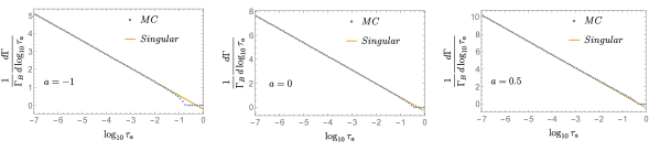
Figure 1: LO MC distribution (dots) and singular distribution (solid line) in gluon channel.

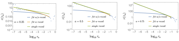
Figure 2: LO nonsingular part (dots) and fit results with and without recoil corrections (blue and orange, respectively) and fit only with recoil corrections

Then, we obtain nonsingular results $r(\tau_{a})$ given in Fig. 2 by taking the difference between MC and singular results. In $a\leq 0$ the nonsingular $r(\tau_{a})$ follows an asymptotic form as

$$\sum_{k=0}^{1}\alpha_{k}\ln^{k}{\tau_{a}}\,.$$ (8)

One can fit with above form to nonsingular part to improve accuracy in small $\tau_{a}$ region when the data suffers from large uncertainties.

On the other hand, in $a>0$ nonsingular part has subleading singular terms that are more significant contributions than those in Eq. (8) and become increasingly large with increasing $a$. According to SCET power counting of angularity, collinear and soft momenta respect following scaling:

$$p_{c}^{\mu}\sim Q\left(\lambda^{2},1,\lambda\right)\quad\text{and}\quad p_{s}^{\mu}\sim Q\lambda^{2-a}\,,$$ (9)

where $\lambda$ is a small parameter in SCET and defined by the observable $\lambda^{2-a}\sim\tau_{a}$. The collinear momentum $p_{c}^{\mu}$ along a unit vector $\hat{n}$ is expressed in the light-cone coordinates and the three components are $n\cdot p_{c}$, $\bar{n}\cdot p_{c}$, and $p_{c}^{\perp}$ where $n=(1,\hat{n})$ and $\bar{n}=(1,-\hat{n})$. For angularity $a\lesssim 0$, the thrust axis is insensitive to transverse recoil by soft radiation, i.e., $p^{\perp}_{c}\gg p^{\perp}_{s}$, but for $a\rightarrow 1$ the recoil effect is significant, i.e., $p^{\perp}_{c}\sim p^{\perp}_{s}$. The recoil corrections obtained from one-loop soft function in Budhraja:2019mcz are given by

$$-\frac{\alpha_{s}C_{i}}{\pi}\frac{4}{2-a}\sum_{n=1}^{\lceil 1/(1-a))\rceil-1}\frac{c_{n}}{\tau_{a}^{1-n(1-a)}}\,,\qquad\left(0<a<1\right)$$ (10)

where the color factor $C_{i}=C_{F}$ and $C_{A}$ for quark and gluon channels, respectively and $\lceil x\rceil$ is the $ceiling\ function$. The series sum turns into a single term $\tfrac{c_{1}}{\tau^{a}}$ for $a\in(0,1/2]$, two terms $\tfrac{c_{1}}{\tau^{a}}+\tfrac{c_{2}}{\tau^{2a-1}}$ for $a\in(1/2,2/3]$, three terms $\tfrac{c_{1}}{\tau^{a}}+\tfrac{c_{2}}{\tau^{2a-1}}+\tfrac{c_{3}}{\tau^{3a-2}}$ for $a\in(2/3,3/4]$, and so on. The recoil corrections are characterized by the fractional power, which is still suppressed compared to the singular terms $\ln^{n}\tau_{a}/\tau_{a}$, but it is greater than typical power corrections $\ln^{n}\tau_{a}$ in Eq. (8). The coefficients $c_{n}$ for $n=1,2,3$ are given by

$$c_{1}=-1,\quad c_{2}=\frac{1}{2}(3-2a),\quad c_{3}=-\frac{1}{6}\left(20-27a+9a^{2}\right)\,.$$ (11)

In our fit, the coefficients are set to free parameters that are determined by the fit to data. The effect of recoil corrections are shown in Fig. 2, where there are three fit results using a form in Eq. (8) without any recoil corrections (blue), a form with both Eq. (8) and Eq. (10) (orange), and a form with just recoil terms in Eq. (10) without Eq. (8) (green). At $a=0.25$ the fit with both terms in Eqs. (8) and (10) works, while at $a=0.5,0.75$ the fit with just recoil terms in Eq. (10) can mostly describe the data. As $a$ increases, the recoil corrections become larger and dominate over typical power corrections in Eq. (8) and the fit without the recoil cannot describe behavior of nonsingular data.

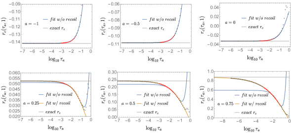
Figure 3: Remainder function (dots) at LO in gluon channel, fit result with and without recoil corrections (blue and orange respectively) to data in fit regions (red).

Fig. 3 shows remainder function $r_{c}(\tau_{a},1)$ (dots) obtained by integrating $r(\tau_{a})$ in Fig. 2, fit curves similar to Fig. 2 and exact value of $r_{c}$ (horizontal gray line) obtained from exact singular part and LO total rate. In selection of fit regions (red) plateau regions are excluded in order to test the prediction of the fit result. The fits with recoil corrections well extrapolate to the exact values of $r_{c}$ in $a>0$, while fits without recoil corrections well extrapolate the exact value in $a\leq 0$ and begin to deviate from the value in $a>0$. The fact that $r_{c}(\tau_{a},1)$ data shows plateau region, which is well aligned with exact value of $r_{c}$ does not motivate such fit and extrapolation since fine-tuning errors in the difference between LO fixed-order and singular part is not significant compared to those at NLO. We again emphasize that the purpose of this subsection is to illustrate significance of including recoil corrections shown the fits and motivate NLO fit with those terms.

3.3 Two-loop constants

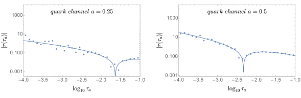
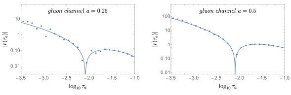
Figure 4: NLO nonsingular parts (dots) at $a=0.25$ and $0.5$ for quark (upper) and gluon (lower) channels and fit curves (blue) including recoil corrections

Following the same strategy, we determine two-loop constant of jet function by using NLO total rate Chetyrkin:1997iv , NLO fixed-order obtained from MC simulations, and two-loop singular part obtained from Eq. (2).

We also perform the fit to nonsingular part by including recoil-correction terms in $a>0$. However, their scaling behavior at NLO is unknown. We make a conjecture for the scaling behavior, test the conjecture in the quark channel then, apply it to the gluon channel. Our conjecture is that dominant scaling behavior can be read from crossing terms between one-loop jet function and recoil corrections from one-loop soft function. In this conjecture we assume that recoil-corrections from two-loop soft function and one- and two-loop jet functions would not produce more singular terms. Convolution of singular terms $\ln^{k}\tau_{a}$ from jet function and recoil corrections of a form in Eq. (10) gives

$$\sum_{n=1}^{\lceil 1/(1-a))\rceil-1}\sum_{k=0}^{2}\,\alpha_{n,k}\frac{\ln^{k}\tau_{a}}{\tau_{a}^{1-n(1-a)}}\,,$$ (12)

where $\alpha_{n,k}$ are fit parameters. For region $0<a\leq 1/2$, $n=1$ and Eq. (12) reduces to

$$\sum_{k=0}^{2}\,\alpha_{1,k}\frac{\ln^{k}\tau_{a}}{\tau_{a}^{a}}\,.\qquad(0<a\leq 1/2)\,.$$ (13)

We also need to include typical integer-power corrections of a form

$$\sum_{k=0}^{3}\alpha_{k}\ln^{k}\tau_{a}\,,$$ (14)

where $\alpha_{k}$ are fit parameters. These terms are leading contributions in $a\leq 0$ since there is no recoil corrections in Eq. (12). The form in Eq. (14) turns into $r_{c}+\tau_{a}\sum_{k=0}^{3}\tilde{\alpha}_{k}\ln^{k}\tau_{a}$ in the remainder function $r_{c}(\tau_{a},1)$ and the value of $r_{c}$ is determined from the fitting to $r_{c}(\tau_{a},1)$ data obtained from Eq. (7).

A subtlety of the fit with recoil corrections in $a>0$ is that eight or, more fit parameters make the fit ill-posed and an ordinary chi-square fit cannot constrain those parameters properly. We adopt Tikhonov regularization tikhonov1963solution , in which a regularization term $\lambda|\Gamma\mathbf{x}|^{2}$ is added to the chi-square and tames the ill-posed fit, where $\lambda$ is a regularization parameter and $\Gamma$ is a Tikhonov matrix. More details about the regularization and our choice of $\lambda$ and $\Gamma$ are discussed in App. D

Fig. 4 shows nonsingular part of angularity distribution in quark and gluon channel at $a=0.25$ and $0.5$ and fitting results using terms in both Eqs. (12) and (14). The fit curves well describe data. We also looked into small $\tau_{a}$ region beyond the range in the figure and checked relative importance of leading-log term in Eq. (12). At $a=0.25$, the fit result with the leading-log alone is qualitatively similar to that with all three terms in Eq. (12). However, at $a=0.5$ just leading-log cannot explain the data and including subleading-log terms in the fit form makes significant improvement. Therefore, we include all three terms in Eq. (12) in our fit.

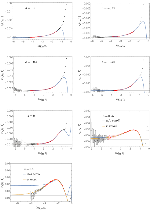
Figure 5: NLO remainder function $r_{c}(\tau_{a},1)$ (gray and red dots with error bar) in quark channel and fit results without recoil corrections (blue) and with the corrections (orange) to selected region of data (red dots with error bar) compared with existing values of $r_{c}$ (horizontal gray line)

Once $r_{c}$ is determined from the fit, one can obtained two-loop constant $c_{\tilde{J}}^{2}$ from following relation

$$r_{c}=-2\left(\frac{\alpha_{s}}{4\pi}\right)^{2}c_{\tilde{J}}^{2}+\Delta_{a}\,,$$ (15)

where $\Delta_{a}=\Gamma_{t}/\Gamma_{B}-\left[A-2\left(\tfrac{\alpha_{s}}{4\pi}\right)^{2}c_{\tilde{J}}^{2}\right]$ is obtained by rewriting Eq. (6) and the term in squared bracket is simply sum of all contributions except for missing $c_{\tilde{J}}^{2}$ hence, is known from the singular part. We determine the constants at seven values of $a=-1+n/4$, where $n=\{0,\cdots,6\}$, for which numerical values of $\Delta_{a}$ for quark and gluon channels are

$$\Delta_{a}^{\text{quark}} = \{-0.0301,-0.0273,-0.0243,-0.0207,-0.0157,-0.0082,0.0036\}\,,$$

$$\Delta_{a}^{\text{gluon}} = \{-0.1598,-0.1474,-0.1319,-0.1106,-0.0787,-0.0258,0.0695\}\,,$$ (16)

where we set $\alpha_{s}=0.1127$.

3.3.1 quark channel

According to procedure described in previous sections, we numerically obtain the remainder function $r_{c}(\tau_{a},1)$ in quark channel at seven values of angularity parameters from $10^{11}$ MC events computed on Intel Xeon Platinum 9242 CPU for about 3k CPU hrs with IR cutoff $\alpha_{\text{cut}}=10^{-11}$ on a dimensionless variable $y_{ij,k}$ in the dipole subtraction Nagy:1998bb ; Nagy:2003tz ; Gleisberg:2007md .

[htb] $c_{\tilde{J}}^{2}\,\textbackslash\,a$ -1 -0.75 -0.5 -0.25 0 this work $65.43\pm 0.91$ $40.41\pm 1.02$ $16.52\pm 0.36$ $-9.10\pm 1.16$ $-36.84\pm 0.72$ Ref. Bell:2018gce $66^{-5.2}_{-3.5}$ $42.3_{-3.3}^{+5.1}$ $17.3_{-2.5}^{+3.2}$ $-9.34_{-2.48}^{+2.76}$ $-36.3_{-2.4}^{+2.7}$ Ref. Brune:2022cgr ^* 67.8 43.1 18.2 $-8.7$ $-34.9$ 0.25 0.5 $-55.36\pm 0.69$ $-3.18\pm 2.13$ $-57.6_{-3.2}^{+3.8}$ $-79.8^{+39.7}_{-24.9}$ $-53.6$ $-0.22$

Table 2: Two-loop constant $c_{\tilde{J}}^{2}$ of quark-jet function for angularity

• The values are read from plots in the thesis and would have errors of a few percent.

The remainder function in Fig. 5 tends to have larger uncertainties in small ${\tau_{a}}$ region around $10^{-4}$ and below, due to fine tuning with large cancellations between fixed-order and singular parts. In the plots for $a\leq 0$ one can read plateau regions approaching existing results Bell:2018gce (horizontal gray line) and determine $r_{c}$ hence, two-loop constant $c_{\tilde{J}}^{2}$ using Eq. (15). The value of $r_{c}$ is determined by extrapolating the fit curve (blue) to $\tau_{a}=0$ with a fit form obtained integrating Eq. (14). In selection of the fit region (red dots with error bar) we eliminated the plateau region to test the asymptotic forms.

On the other hand, in $a>0$ a plateau is hardly observed from data and two fit results with and without recoil corrections (orange and blue) are shown in the figure, respectively. Plateau region would appear smaller $\tau_{a}$ region as $a$ increases because the recoil corrections like $\tau_{a}^{n(1-a)}$ make convergence of the remainder functions further slow. It is not accessible from MC results computed with double precision of machine variables. As indicated in Fig. 4, the fit with recoil corrections at $a=0.5$ clearly extrapolate to the value of $r_{c}$ close to existing value Brune:2022cgr (horizontal gray line). Our values of $c_{\tilde{J}}^{2}$ is given in Table 2 and show reasonable agreement existing results in Bell:2018gce ; Brune:2022cgr . We note that our fit region does not include plateau region and our results in Table 2 tend would have larger uncertainties than those that could have been obtained from the best fit including the plateau region because our purpose in the quark channel is to verify fitting with the asymptotic form.

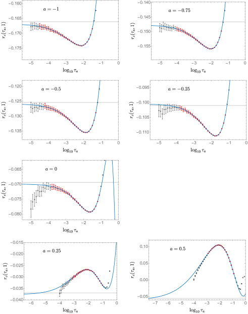
Figure 6: NLO remainder function $r_{c}(\tau_{a},1)$ (gray and red dots with error bar) in gluon channel and fit results (blue) to selected region of data (red dots with error bar) compared with existing values of $r_{c}$ (horizontal gray line)

In the fit region (red dots with error bar), we take a set of fit regions $\{\tau_{a}^{\text{low}}\,,\tau_{a}^{\text{high}}\}$ and obtain a set of $r_{c}$ values and statistical uncertainties from fitting to the regions. For a systematic uncertainty that would mainly come from IR cutoff and higher-power corrections we take a maximum deviation of $r_{c}$ from its averaged value in the set. We obtain our central value from the averaged $r_{c}$ and our uncertainty from sum of the systematic and averaged-statistical uncertainties in quadrature. Specifically, the set $\{\tau_{a}^{\text{low}}\,,\tau_{a}^{\text{high}}\}$ is obtained from all possible combinations for the pair from 9 succeeding points for $\log_{10}\tau_{a}^{\text{low}}$ domain separated by a step size of $0.1$ and similarly 5 succeeding points for $\log_{10}\tau_{a}^{\text{high}}$ domain. Our selection criteria for $\tau_{a}^{\text{high}}$ domain is that it should be robust against higher-power corrections and we select $\{-1.6+0.4(1+a),-1.2+0.4(1+a)\}$. The criteria for $\tau_{a}^{\text{low}}$ domain is that it should be insensitive to IR cutoff and we scan all available domains of 9 succeeding points and select the domain giving least standard deviation for $r_{c}$. We also explore the effect of the cutoff $\alpha_{\text{cut}}$ by comparing our standard value $\alpha_{\text{cut}}=10^{-11}$ and larger value $10^{-8}$ in App. E

3.3.2 gluon channel

[b] $c_{\tilde{J}}^{2}\,\textbackslash\,a$ -1 -0.75 -0.5 -0.25 0 this work $44.19\pm 1.70$ $2.10\pm 2.75$ $-36.43\pm 1.65$ $-62.08\pm 2.49$ $-54.55\pm 2.60$ Ref. Brune:2022cgr ^* $37.18$ $-4.59$ $-40.27$ $-56.95$ $-55.73$ $c_{\tilde{J}}^{2}\,\textbackslash\,a$ 0.25 0.5 this work $75.09\pm 10.99$ $814.48\pm 28.71$ Ref. Brune:2022cgr ^* $69.21$ $776.61$

Table 3: two-loop constant $c_{\tilde{J}}^{2}$ of gluon-jet function for angularity

• The values are read from plots in the thesis and would have errors of a few percent.

Now we determine two-loop constant of angularity gluon-jet function and compare our results to values given in Brune:2022cgr . The procedure is essential same as that described in Sec. 3.3.1 and we only describe the difference from the section.

We use the same number of $10^{11}$ MC events with larger cutoff $\alpha_{\text{cut}}=10^{-8}$ in the gluon channel. Fig. 6 shows NLO remainder function $r_{c}(\tau_{a},1)$ (gray and red dots with error bar) obtained from MC events compared with fit results (blue) to selected region of data (red dots) and $r_{c}$ values in Brune:2022cgr (horizontal gray line). The fits in $a\leq 0$ were performed without the recoil corrections and in $a>0$ with the recoil corrections. Unlike the quark channel, we do not observe any plateau regions at any value of $a$ hence, fitting with asymptotic form in Eqs. (12) and (14) is essential in the gluon channel.

Due to more severe cutoff effect the fit regions are narrowed and domains of $\log_{10}\tau_{a}^{\text{low}}$ reduces to 7 succeeding points for non-positive $a$ and $\log_{10}\tau_{a}^{\text{high}}$ to 5 points for positive $a$. Cutoff effect on the value of $c_{\tilde{J}}^{2}$ in the gluon channel is shown in App. E.

Table 3 shows our two-loop constant $c_{\tilde{J}}^{2}$ converted from $r_{c}$ values by using Eq. (15) and our values show reasonable agreement with the values in Brune:2022cgr .

4 Angularity distributions at $\text{NNLL}^{{}^{\prime}}$ matched to NLO

In this section we present the angularity distribution at $\text{NNLL}^{{}^{\prime}}$ matched to fixed-order NLO results, which is $\mathcal{O}(\alpha_{s}^{2})$ corrections relative to the born rate $\Gamma_{B}(\mu)$. The distribution is composed of two parts as

$$\frac{1}{\Gamma_{B}}\frac{d\Gamma}{d\tau_{a}}=\frac{1}{\Gamma_{B}}\frac{d\Gamma^{\text{res}}}{d\tau_{a}}+r(\tau_{a},\mu_{\text{ns}})\,,$$ (17)

where $\tfrac{d\Gamma^{\text{res}}}{d\tau_{a}}$ is resummed-singular part and $r(\tau_{a},\mu_{\text{ns}})$ is the nonsingular part at a scale $\mu_{\mathrm{ns}}$ including all subleading-power corrections of $\tau_{a}$ at NLO. As described in Sec. 2 by RG evolving the functions in factorization in Eq. (3), we perform the log resummation, detailed procedure of which is summarized in App. A and App. B with a final expression in Eq. (54). The nonsingular part makes our full distribution in Eq. (17) matched to fixed-order result as is defined as Eq. (5). Including this is important because unphysical behavior of singular terms in large $\tau_{a}$ region can be corrected by adding nonsingular part. Note that in Eq. (17) $\Gamma_{B}=\Gamma_{B}(m_{H})$ is the born decay rate at the scale of Higgs mass hence, both the singular and nonsingular parts contain a prefactor $\Gamma_{B}(\mu)/\Gamma_{B}(m_{H})=\alpha_{s}(\mu)^{2}/\alpha_{s}(m_{H})^{2}$.

We also compute a cumulative distribution by integrating Eq. (17) from 0 to $\tau_{a}$ as

$$\frac{\Gamma_{c}\left(\tau_{a}\right)}{\Gamma_{B}}=\int_{0}^{\tau_{a}}d\tau_{a}^{\prime}\left[\frac{1}{\Gamma_{B}}\frac{d\Gamma^{\text{res}}}{d\tau_{a}^{\prime}}+r(\tau_{a}^{\prime})\right]=\frac{\tau_{a}}{\Omega\,\Gamma_{B}}\frac{d\Gamma^{\text{res}}}{d\tau_{a}}+r_{c}(0,\tau_{a})\,,$$ (18)

where $\Omega=\eta_{S}+2\eta_{J}$ is the sum of integrated anomalous dimensions of jet and soft function, which are defined in Eqs. (40) and (41). When the resummation is turned off, $\Omega$ reduces to zero and cancels against the same factor in $d\Gamma^{\text{res}}/d\tau_{a}$ so that $\Gamma_{c}(\tau_{a})$ remains finite.

4.1 Matching

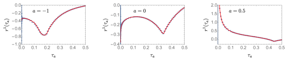
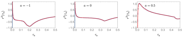
Figure 7: LO (upper) and NLO (lower) coefficients of nonsingular part $r\left(\tau_{a},\mu_{\mathrm{ns}}\right)$ at $a=-1,\,0,\,0.5$.

The nonsingular part in Eq. (17) can be expressed in a scale independent form satisfying $dr\left(\tau_{a},\mu\right)/d\mu=0$ as

$$r\left(\tau_{a},\mu_{\mathrm{ns}}\right)=\frac{\alpha_{s}(\mu_{\mathrm{ns}})^{2}}{\alpha_{s}(m_{H})^{2}}\left\{\frac{\alpha_{s}\left(\mu_{\mathrm{ns}}\right)}{4\pi}r^{1}\left(\tau_{a}\right)+\left(\frac{\alpha_{s}\left(\mu_{\mathrm{ns}}\right)}{4\pi}\right)^{2}\left[r^{2}\left(\tau_{a}\right)+3\beta_{0}r^{1}\left(\tau_{a}\right)\ln\frac{\mu^{2}_{\mathrm{ns}}}{m_{H}^{2}}\right]\right\}\,,$$ (19)

where $r^{1}(\tau_{a})$ and $r^{2}(\tau_{a})$ are LO and NLO coefficients, respectively and only depend on $\tau_{a}$. The scale dependency on $\mu_{\mathrm{ns}}$ is made explicit with the logarithmic term proportional $3\beta_{0}r^{1}$, which is cancelled by the same term generated by scale variation of lower-order term proportional to $r^{1}(\tau_{a})$. In comparison to nonsingular part in $e^{+}e^{-}$ angularity Bell:2018gce , the log term differs from that in Bell:2018gce by a factor of 3 due to additional prefactor $\alpha_{s}(\mu_{\mathrm{ns}})^{2}$ from the born rate $\Gamma_{B}^{g}(\mu)$, which is absent in $e^{+}e^{-}$ angularity.

An analytic expression of the nonsingular part is unknown except for the thrust limit $a=0$, and it is determined numerically from MC events obtained in Sec. 3.3. We interpolate the remainder function obtained from MC events instead of interpolating nonsingular part because binned-nonsingular part inherit uncertainties by an amount of bin size in x-axis associated while its integration, remainder function, does not at the end of each bin. Then, we obtain the nonsingular part by taking numerical differentiation of interpolated remainder function.

In order to maintain good precision of the interpolation in both small and large $\tau_{a}$ regions, the spectrum of $r^{n}(\tau_{a})$ is divided into two regions, below and above a point $\tau_{a}=0.1$. Below the point, MC data is binned in log space from a lower bound $\log_{10}\tau_{a}^{\text{low}}$ to the point with a step size of $0.1$, where the lower bound is $-7$ at LO and $-4$ or, $-5$ at NLO. Above the point the MC data is binned in linear space $\tau_{a}$ up to $1$ with a step size of $0.01$. At NLO, MC data in small $\tau_{a}$ regions tends to be significantly biased by the cutoff effect as shown in Fig. 11, and the fit function is instead to describe points below $\tau_{a}=0.1$. At NLO, MC data in small $\tau_{a}$ regions tends to be significantly biased by the cutoff effect as shown in Fig. 11, and the fit function is instead to describe points below $\tau_{a}=0.1$. Then, interpolation functions $r_{\log_{10}}^{n}(\tau_{a})$ and $r_{\operatorname{lin}}^{n}(\tau_{a})$ in two regions are joined smoothly following the method in Bell:2018gce :

$$r^{n}\left(\tau_{a}\right)=\left[1-f\left(\tau_{a},0.1,0.01\right)\right]r_{\log_{10}}^{n}\left(\tau_{a}\right)+f\left(\tau_{a},0.1,0.01\right)r_{\operatorname{lin}}^{n}\left(\tau_{a}\right)\,,$$ (20)

where $f\left(z,z_{0},\epsilon\right)=1/\left(1+e^{-\left(z-z_{0}\right)/\epsilon}\right)$ is a transition function.

Nonsingular distributions with error bars at LO (first row) and at NLO (second row) are shown in Fig. 7, and red curves are the interpolations joined using Eq. (20). Note that the nonsingular is not physical quantity and can be negative, while full distribution in Eq. (17) is physical and positive definite.

4.2 Numerical results

For the numerical calculation of distribution one needs to make proper choice for the scales: hard scales $\mu_{C_{t}}$, $\mu_{C_{S}}$, soft scale $\mu_{S}$ and jet scale $\mu_{J}$. In the choice one needs to consider $\tau_{a}$ distribution divided by three regions: the peak region $\left(\tau_{a}\sim 2\Lambda_{QCD}/m_{H}\ll 1\right)$, the tail region $\left(2\Lambda_{QCD}/m_{H}\ll\tau_{a}\ll 1\right)$ and the far-tail region $(\tau_{a}\sim 1)$. The tail region is the region where $\tau_{a}$ remains small and resummation is effective. In the region, natural choice is the canonical scales $\mu_{C_{t},C_{S}}=m_{H},\,\mu_{J}=m_{H}\tau_{a}^{1/(2-a)},\,\mu_{S}=m_{H}\tau_{a}$ that minimize the logarithms in each function. In far-tail region, $\mu_{i}\!\sim\!\mathcal{O}(m_{H})$ and we can set all scales to be hard scale $\mu_{i}=m_{H}$, which is a conventional choice in fixed-order perturbation theory. The peak region is dominated by nonperturbative (NP) effect and our perturbative approach is invalid. Before approaching the peak region, we need to stop scales running into $\Lambda_{QCD}$ and make them frozen in perturbative region well above $\Lambda_{QCD}$ . One can design Profile function $\mu_{i}(\tau_{a})$ that is a smooth function of $\tau_{a}$ satisfying above criteria Abbate:2010xh ; Ligeti:2008ac ; Berger:2010xi . Here, we adopt the profile functions and scale variations to estimate perturbative uncertainty designed for the $e^{+}e^{-}$ angularity in Bell:2018gce and we modify a parameter $t_{2}(a)$ to be $0.43\times 0.674^{1-1.913a}$, which is the value of $\tau_{a}$ where singular and nonsingular parts of gluon channel are the same in size and beyond the point all scales smoothly transit to the hard scale. We also take the choice of Bell:2018gce for a scale $\mu_{\mathrm{ns}}$ in nonsingular part.

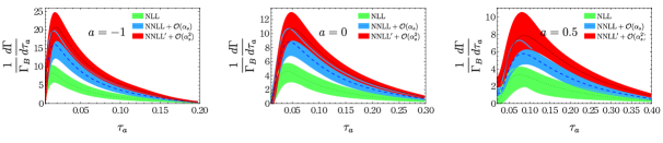
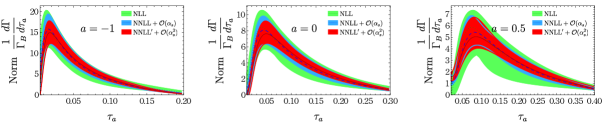
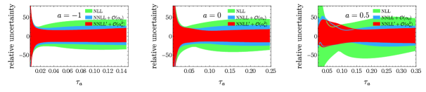
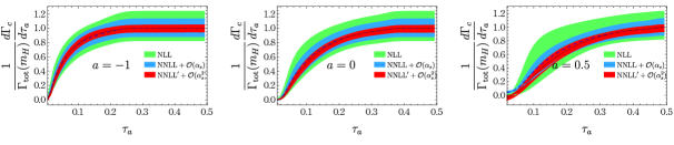
Figure 8: First and second rows: Angularity distributions at three values of $a=-1,\,0,\,0.5$ for gluon channel in Higgs decay. The bands indicate perturbative uncertainties. The first row is normalized by the born rate and the second by total rate at corresponding order. Third row: Relative perturbative uncertainty in percentage. Bottom row: Cumulative distributions normalized by total rate.

Fig. 8 shows our resummed results at $\text{NNLL}^{{}^{\prime}}$ $+\mathcal{O}(\alpha_{s}^{2})$ accuracy (red) for angularity distribution (first and second rows), relative uncertainties (third row), and cumulative distributions (fourth row) at three values of $a=-1$, 0, and 0.5 and results at lower accuracies: NLL (green) and NNLL$+O(\alpha_{s})$ (blue) for a comparison. Band at each accuracy represents perturbative uncertainty estimated by scale variations in the profile function. The distributions normalized by the born rate in first row hardly overlap between different accuracies and the peak of distribution increase by $100~{}\%$ from NLL to NNLL and $50~{}\%$ from NNLL to $\text{NNLL}^{{}^{\prime}}$ because of large perturbative corrections as in the total rate. The distributions normalized by their own area in second row show reasonable overlapping within the uncertainties between different accuracies which indicates a perturbative convergence of the resummation. In the third row, the perturbative uncertainties with respect to central values reduce to about $20~{}\%$ at $\text{NNLL}^{{}^{\prime}}$ , which is about half of NLL uncertainties, however the reduction rate with increasing accuracy is rather slow compared to the quark channel as many gluon initiated processes do. $c_{\tilde{J}}^{2}$ uncertainties in Table 3 propagate to the distribution and are as large as $0.7\%$, which is negligible compared to the perturbative uncertainties at this level of accuracy. In fourth row the cumulative distribution is normalized by the total rate at corresponding order in $\alpha_{s}$. One can observe the cumulative distribution reduces to the total rate in the far-tail region. In the region resummation is returned off and resummed distribution in Eq. (17) reduces to the fixed-order result in Eq. (5).

One can observe a generic feature of distribution that the shape becomes broad and the peak moves to right with increasing $a$ because for a given jet scale $\mu_{J}=m_{H}\tau_{a}^{1/(2-a)}$, increasing $a$ scales up value of $\tau_{a}$. But this is not true for the soft scale $\mu_{S}=m_{H}\tau_{a}$, where $a$ does not change the scale of $\tau_{a}$. Both of them affect the distribution and make its change as a function of $a$ nontrivial. The peak of distribution is essential feature of the resummation known as Sudakov exponent that is $e^{-\frac{2\alpha_{s}C_{A}}{\pi}\ln^{2}\tau_{a}}$ at LL accuracy, which cures the singular behavior $\ln\tau_{a}/\tau_{a}$ and the peak position of gluon channel is rather located at large $\tau_{a}$ compared to that in the quark channel due to the Casimir scaling.

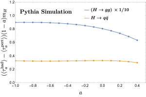
Figure 9: Difference between $\langle\tau_{a}^{\text{had}}\rangle$ at hadron level and $\langle\tau_{a}^{\text{pert}}\rangle$ at parton level from Pythia simulation for gluon channel (blue) and for quark channel (orange).

Fig. 8 shows pure perturbative contribution without the NP effect like hadronization that can be included by introducing a NP model Ligeti:2008ac ; Kang:2013nha ; Kang:2014qba or, power correction with a universal NP parameter $\Omega\sim\mathcal{O}(\Lambda_{\text{QCD}})$ Lee:2006nr , which can be further refined with a scheme subtracting renormalon ambiguities Hoang:2007vb ; Hoang:2008fs . The parameter $\Omega$ captures a leading NP correction and shifts the perturbative distribution, hence first moment of $\tau_{a}$ as

$$\langle\tau_{a}^{\text{had}}\rangle=\langle\tau_{a}^{\text{pert}}\rangle+\frac{2}{1-a}\frac{\Omega}{m_{H}}+\mathcal{O}(\Lambda_{\text{QCD}}^{2}/m_{H}^{2})\,,$$ (21)

where the superscript ‘had’ is for the hadron level that can be measured in experiment or, simulated in event generators and ‘pert’ is for pure perturbative result at the parton level. Eq. (21) includes quark and gluon channels $\Omega=f_{q}\Omega_{q}+f_{g}\Omega_{g}$, where $f_{i}=\Gamma^{i}_{tot}/(\Gamma^{q}_{tot}+\Gamma^{g}_{tot})\approx 0.9$ and $0.1$ the quark and gluon fractions, respectively. For the quark channel $\Omega_{q}^{ee}\approx 0.35$ GeV from $e^{+}e^{-}$ thrust analysis Abbate:2010xh and assuming Casimir scaling estimates $\Omega_{g}\approx C_{A}/C_{F}\Omega_{q}$. We can determine $\Omega_{g}$ in Higgs factories by using the known value of $\Omega_{q}^{ee}$.

Eq. (21) predicts $a$ dependence $(1-a)^{-1}$ in $\Omega$ term that can be easily identified by comparing experiment and theory predictions in $a$ space Berger:2003pk . We can also test if $a$ dependence in $\Omega$ term is comparable with hadronization model in event generators. Fig. 9 shows the difference $\langle\tau_{a}^{\text{had}}\rangle-\langle\tau_{a}^{\text{pert}}\rangle$ with a weight $(1-a)m_{H}$ obtained from Pythia simulations for the quark channel and gluon channel. $y$ values corresponds to $2\Omega$ for the quark and $2\Omega/10$ for the gluon and would weakly depend on $a$ via subleading term $\mathcal{O}(\Lambda_{\text{QCD}}^{2}/m_{H}^{2})$ in Eq. (21). While the quark channel is consistent with the $a$ dependence and $\Omega_{q}^{\text{pythia}}\approx 0.2$ GeV roughly agreeing with $\Omega_{q}^{ee}$ within a factor of two, the gluon channel shows rather stronger $a$ dependence and indicates $\Omega_{g}^{\text{pythia}}\approx 3\sim 5$ GeV greater than $\Lambda_{\text{QCD}}$ by an order of magnitude. Interestingly, their relative contributions are not much different $f_{q}\Omega_{q}\text{pythia}\approx 0.2$ and $f_{g}\Omega_{g}^{\text{pythia}}\approx 0.3\sim\!0.5$. Measurements in future Higgs factories would justify the value of $\Omega_{g}$. If Pythia value is different from the measurement, it could come from another source such as large perturbative corrections at higher orders absent in Pythia that have been absorbed into hadronization parameters fitted to experimental data.

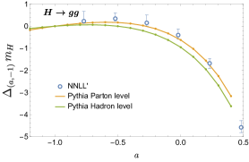
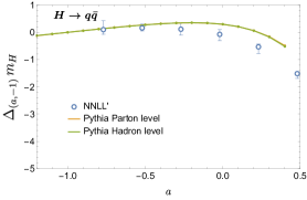
Figure 10: Prediction of subtracted moment $\Delta_{(a,-1)}$ as a function of $a$ from resummed results at NLL and $\text{NNLL}^{{}^{\prime}}$ compared with Pythia simulations at parton and hadron levels for quark channel (left) and for gluon channel (right)

The subleading NP corrections of $\mathcal{O}(\Lambda_{\text{QCD}}^{2}/m_{H}^{2})$ in Eq. (21) can be studied from higher-moment or, cumulant analysis. In $e^{+}e^{-}$ thrust Abbate:2012jh , 2nd thrust cumulant, which is completely insensitive to $\Omega^{q}$ enabled to determine a subleading correction $\Omega_{2}^{{}^{\prime}q}(0)$, which is the sum of two contributions, one from leading thrust factorization and the other from a power correction $\Omega^{q}_{1,1}(0)\sim\Lambda_{\text{QCD}}^{2}$ multiplied by a perturbative part. This can be extended to $e^{+}e^{-}$ angularity to determine $\Omega_{2}^{{}^{\prime}q}(a)$ at nonzero $a$ and to angularity in Higgs decay to determine corresponding corrections in the gluon channel. Following the convention of Abbate:2012jh , the correction $\mathcal{O}(\Lambda_{\text{QCD}}^{2}/m_{H}^{2})$ in Eq. (21) can be parameterized as $2M_{0,1}(a)\,\Omega_{1,1}(a)/m_{H}^{2}$, where $\Omega_{1,1}(a)$ is the correction appeared in the 2nd cumulant and $M_{0,1}(a)$ accounts for a perturbative part. Another way to study the subleading NP corrections is to take the difference between moments as in Chien:2018lmv ; Kang:2018agv at two points in $a$ space

$$\Delta_{(a,a^{\prime})} = (1-a)\langle\tau_{a}^{\text{had}}\rangle-(1-a^{\prime})\langle\tau_{a^{\prime}}^{\text{had}}\rangle$$ (22)

$$= (1-a)\langle\tau_{a}^{\text{pert}}\rangle-(1-a^{\prime})\langle\tau_{a^{\prime}}^{\text{pert}}\rangle+\mathcal{O}(\Lambda_{\text{QCD}}^{2}/m_{H}^{2})\,,$$

where the leading correction $\Omega$ is cancelled in second line and the subtracted moment $\Delta_{(a,a^{\prime})}$ is sensitive to the subleading correction that can be expressed as a difference of the quantity $2(1-a)M_{0,1}(a)\,\Omega_{1,1}(a)/m_{H}^{2}$ at two points $a$ and $a^{\prime}$. By comparing experimental measurement and perturbative predictions one can determine the correction. The subtracted moment with angularity provides additional information different from that obtained from thrust cumulant analysis hence, is a useful tool for extracting information on subleading NP corrections. Fig. 10 shows our perturbative predictions of Eq. (22) at $\text{NNLL}^{{}^{\prime}}$ accuracies compared with Pythia simulations at parton and hadron levels for the gluon channel (left) and the quark channel (right). The Pythia results in gluon channel show a notable difference between parton and hadron levels, while the difference in quark channel is very small. This analysis can be done for different colliders such as Electron-Ion Collider AbdulKhalek:2021gbh with DIS trust and angularity Kang:2013nha ; Kang:2014qba ; Chu:2022jgs ; Zhu:2021xjn and determine NP corrections.

5 Conclusion

We present improved predictions of angularity distribution $\tau_{a}$ in hadronic decays of Higgs boson via effective operator $H\to gg$ that suffers from large perturbative uncertainties compared to the other contribution via Yukawa interaction $H\to q\bar{q}$. The distribution is improved by resumming large logarithms of angularity at $\text{NNLL}^{{}^{\prime}}$ accuracy in the frame work of SCET and by matching the resummed results to the fixed-order result at NLO.

In order to achieve $\text{NNLL}^{{}^{\prime}}$ accuracy, we independently determined a remaining ingredient, 2-loop constant of gluon-jet function for angularity. We find our values of the constant show reasonable agreement with the values in literature. In the determination of the constant, there is significant contamination from subleading singular corrections slowly suppressed in small $\tau_{a}$ limit. In order to estimate the correction, we use asymptotic forms in small $\tau_{a}$ region and fit it to the nonsingular part of fixed-order result. The asymptotic form for $a\leq 0$ is $\sum_{k}\alpha_{k}\ln^{k}\tau_{a}$, which is one power-suppressed by the singular part and for $0<a\leq 1/2$ it has additional terms with fractional power $\sum_{k}\alpha_{1,k}\ln^{k}\tau_{a}/(\tau_{a})^{a}$, which is conjectured from recoil corrections in one-loop soft function. The form in $a>0$ has eight degrees of freedom and fitting result is sensitive to noise hence, ill-posed. We found that it can be handled by adopting a Tikhonov regularization that reduces the sensitivity to noise.

We also consider nonperturbative corrections in the angularity. The corrections receive two contributions one from quark channel and the other from gluon channel and by using the value known for the quark in $e^{+}e^{-}$ experiment, the gluon contribution can be determined from measurement in Higgs factories. Pythia simulation shows that the quark channel is comparable to prediction of leading-power correction for the angularity, while the gluon channel is quiet different the prediction in $a$ dependency and magnitude estimated from Casimir scaling. We also considered subtracted moment $\Delta_{(a,a^{\prime})}$ defined by difference between moments of $\tau_{a}$ at $a$ and $a^{\prime}$ that mitigates the leading correction hence, is sensitive to subleading corrections. The subtracted moment as a function of $a$ is an independent direction from the cumulant analysis and provides additional information to the subleading correction.

Appendix A SCET functions

Here, we summarize the functions appear in the factorization in the gluon channel and the tag $g$ representing the gluon is implied implicit. In Laplace space each function $G=\{C_{t},C_{S},\tilde{J},\tilde{S}\}$ in Eq. (3) can be expressed as:

$$G\left(L_{G},\mu_{G}\right)= \sum_{n=0}^{\infty}\left(\frac{\alpha_{s}\left(\mu_{G}\right)}{4\pi}\right)^{n}G^{(n)}\left(L_{G}\right)$$ (23)

$$G^{(0)}\left(L_{G}\right)= 1$$

$$G^{(1)}\left(L_{G}\right)= \left[\Gamma_{G}^{0}L_{G}^{2}-\gamma_{G}^{0}L_{G}+c_{G}^{1}\right]$$

$$G^{(2)}\left(L_{G}\right)= \left[\frac{1}{2}\left(\Gamma_{G}^{0}\right)^{2}L_{G}^{4}-\Gamma_{G}^{0}\left(\gamma_{G}^{0}+\frac{2}{3}\beta_{0}\right)L_{G}^{3}\right.$$

$$\left.+\left(\Gamma_{G}^{1}+\frac{1}{2}\left(\gamma_{G}^{0}\right)^{2}+\gamma_{G}^{0}\beta_{0}+c_{G}^{1}\Gamma_{G}^{0}\right)L_{G}^{2}-\left(\gamma_{G}^{1}+c_{G}^{1}\gamma_{G}^{0}+2c_{G}^{1}\beta_{0}\right)L_{G}+c_{G}^{2}\right]\,,$$

where $\Gamma_{G}^{n}=-\frac{j_{G}\kappa_{G}}{2}\Gamma_{n}$. $\Gamma_{n}$, $\gamma_{G}^{n}$, $c_{G}^{n}$ are coefficients of the universal cusp and non-cusp anomalous dimensions $\Gamma_{\text{cusp}}(\alpha_{s})$ and $\gamma_{G}(\alpha_{s})$ and of a constant term $c_{G}$ in $\alpha_{s}$ expansion as

$$\Gamma_{\text{cusp}}(\alpha_{s})=\sum_{n=0}\Gamma_{n}\,\left(\frac{\alpha_{s}}{4\pi}\right)^{n+1}\,,\quad\gamma_{G}(\alpha_{s})=\sum_{n=0}\gamma_{G}^{n}\,\left(\frac{\alpha_{s}}{4\pi}\right)^{n+1}\,,\quad c_{G}=\sum_{n=1}c_{G}^{n}\,\left(\frac{\alpha_{s}}{4\pi}\right)^{n}\,,$$ (24)

where $\beta_{n}$ and $\Gamma_{n}$ are given in App. C and $\gamma_{G}^{n}$, and $c_{G}^{n}$ are given in App. A.1 and App. A.2, respectively. The factors $j_{G}$ and $\kappa_{G}$ and log $L_{G}$ are summarized in Table 4.

$$\begin{array}[]{c|cccccc}\hline\cr&C_{t}&C_{S}&\tilde{J}&\tilde{S}\\ \hline\cr j_{G}&1&1&2-a&1\\ \hline\cr\kappa_{G}&0&2&-2/(1-a)&4/(1-a)\\ \hline\cr L_{G}&\ln\frac{m_{t}}{\mu_{C_{t}}}&\ln\frac{im_{H}}{\mu_{C_{S}}}&\ln\left[\frac{m_{H}}{\mu_{\tilde{J}}}\left(\nu e^{\gamma_{E}}\right)^{-1/j_{\tilde{J}}}\right]&\ln\left[\frac{m_{H}}{\mu_{\tilde{S}}}\left(\nu e^{\gamma_{E}}\right)^{-1/j_{\tilde{S}}}\right]\\ \hline\cr\end{array}$$

Table 4:

The each term Eq. (23) can be transformed into the momentum space by the inverse Laplace transformation as following:

$$1 \rightarrow\delta(\tau)$$ (25)

$$-\ln\nu e^{\gamma_{E}} \rightarrow\mathcal{L}_{0}(\tau)$$

$$\ln^{2}\nu e^{\gamma_{E}} \rightarrow 2\mathcal{L}_{1}(\tau)-\frac{\pi^{2}}{6}\delta(\tau)$$

$$-\ln^{3}\nu e^{\gamma_{E}} \rightarrow 3\mathcal{L}_{2}(\tau)-\frac{\pi^{2}}{2}\mathcal{L}_{0}(\tau)+2\zeta_{3}\delta(\tau)$$

$$\ln^{4}\nu e^{\gamma_{E}} \rightarrow 4\mathcal{L}_{3}(\tau)-2\pi^{2}\mathcal{L}_{1}(\tau)+8\zeta_{3}\mathcal{L}_{0}(\tau)+\frac{\pi^{4}}{60}\delta(\tau)\,,$$

where the distribution function $\mathcal{L}_{n}(\tau)$ is defined by

$$\mathcal{L}_{n}(\tau) =\begin{cases}\left[\frac{\ln^{n}(\tau)}{\tau}\right]_{+}&\quad n\geq 0\,,\\ \delta(\tau)&\quad n=-1.\end{cases}$$ (26)

A.1 Non-cusp anomalous dimension

The anomalous dimension of the function $G$ is defined by the Renormalization Group (RG) equation as

$$\mu\frac{d}{d\mu}G(\nu,\mu)=\gamma_{G}(\mu)G(\nu,\mu)\,,$$ (27)

$$\gamma_{G}(\mu)=j_{G}\kappa_{G}\Gamma_{\text{cusp }}\left(\alpha_{s}\right)L_{G}+\gamma_{G}\left(\alpha_{s}\right)$$ (28)

From scale independence of the factorization in Eq. (3), we have a consistence relation:

$$\frac{2\beta(\alpha_{s})}{\alpha_{s}}+2\gamma_{C_{t}}(\alpha_{s})+2\gamma_{C_{s}}(\alpha_{s})+2\gamma_{J}(\alpha_{s})+\gamma_{S}(\alpha_{s})=0$$ (29)

where the first term is from the born rate $\Gamma_{B}\propto\alpha_{s}^{2}$. The non-cusp anomalous dimensions of $C_{t}$inami1983effective ; djouadi1992higgs ; Chetyrkin:1997iv ; Chetyrkin:1997un ; Chetyrkin:2005ia ; baikov2017five and $C_{S}$ Gehrmann:2010ue are given by

$$\gamma_{C_{t}}^{0} =0\,,\qquad\gamma_{C_{t}}^{1}=-2\beta_{1}\,,$$ (30)

$$\gamma_{C_{S}}^{0} =0\,,\qquad\gamma_{C_{S}}^{1}=\left(-\frac{118}{9}+4\zeta_{3}\right)C_{A}^{2}+\left(-\frac{38}{9}+\frac{\pi^{2}}{3}\right)C_{A}\beta_{0}+2\beta_{1}\,,$$

The quark soft anomalous dimension is given in Hornig:2009vb ; Bell:2018vaa , gluon soft anomalous dimension can be obtained from quark soft anomalous dimension by a Casimir scaling that is $C_{F}\to C_{A}$.

$$\gamma_{S}^{0}(a)=0\,,\qquad\gamma_{S}^{1}(a)=\frac{2}{1-a}\left[\gamma_{1}^{CA}(a)C_{A}^{2}+\gamma_{1}^{nf}(a)C_{A}T_{F}n_{f}\right]\,,$$ (31)

where we have made the $a$-dependence of the anomalous dimension explicit, and

$$\gamma_{1}^{CA}(a) =-\frac{808}{27}+\frac{11\pi^{2}}{9}+28\zeta_{3}-\Delta\gamma_{1}^{CA}(a)\,,$$ (32)

$$\gamma_{1}^{nf}(a) =\frac{224}{27}-\frac{4\pi^{2}}{9}-\Delta\gamma_{1}^{nf}(a)\,,$$

where

$$\Delta\gamma_{1}^{CA}(a) =\int_{0}^{1}dx\int_{0}^{1}dy\frac{32x^{2}\left(1+xy+y^{2}\right)\left[x\left(1+y^{2}\right)+(x+y)(1+xy)\right]}{y\left(1-x^{2}\right)(x+y)^{2}(1+xy)^{2}}\ln\left[\frac{\left(x^{a}+xy\right)\left(x+x^{a}y\right)}{x^{a}(1+xy)(x+y)}\right],$$ (33)

$$\Delta\gamma_{1}^{nf}(a) =\int_{0}^{1}dx\int_{0}^{1}dy\frac{64x^{2}\left(1+y^{2}\right)}{\left(1-x^{2}\right)(x+y)^{2}(1+xy)^{2}}\ln\left[\frac{\left(x^{a}+xy\right)\left(x+x^{a}y\right)}{x^{a}(1+xy)(x+y)}\right],$$

which vanish for thrust case $a=0$. Here we give numerical result at the values of $a$ used in MC simulation.

$a$	$-1.0$	$-0.75$	$-0.5$	$-0.25$	$0.0$	$0.25$	$0.5$
$\gamma_{1}^{CA}$	$1.0417$	$5.8649$	$9.8976$	$13.190$	$15.795$	$17.761$	$19.132$
$\gamma_{1}^{nf}$	$-0.9571$	$0.5284$	$1.8440$	$2.9751$	$3.9098$	$4.6398$	$5.1613$

Then, we can obtain $\gamma_{J}(\alpha_{s})$ is given by Eq. (29).

A.2 Constant term

Content terms in $C_{t}$ inami1983effective ; djouadi1992higgs ; Chetyrkin:1997iv ; Chetyrkin:1997un ; Chetyrkin:2005ia ; baikov2017five and $C_{S}$ Gehrmann:2010ue are given by

$$c_{C_{t}}^{1}=11,$$ (34)

$$c_{C_{t}}^{2}=\frac{2777}{18}-\frac{67}{6}n_{f},$$

$$c_{C_{S}}^{1}=C_{A}\frac{\pi^{2}}{6},$$

$$c_{C_{S}}^{2}=C_{A}^{2}\left(\frac{\pi^{4}}{72}-\frac{143\zeta_{3}}{9}+\frac{67\pi^{2}}{36}+\frac{5105}{162}\right)+C_{F}n_{f}\left(8\zeta_{3}-\frac{67}{6}\right)+C_{A}n_{f}\left(-\frac{46\zeta_{3}}{9}-\frac{5\pi^{2}}{18}-\frac{916}{81}\right)\,.$$

The constant term of quark soft functions is known to one-loop for generic values of $a$ analytically Hornig:2009vb , the two-loop constant is determined numerically for generic $a$ in Bell:2020yzz . Gluon soft function can be obtained from quark soft function constant by a Casimir scaling that is $C_{F}\to C_{A}$. In Laplace space:

$$c_{\tilde{S}}^{1}(a)=-C_{A}\frac{\pi^{2}}{1-a}\,,$$ (35)

$$c_{\tilde{S}}^{2}(a)=c_{2}^{CA}(a)C_{A}^{2}+c_{2}^{nf}(a)C_{A}T_{F}n_{f}+\frac{\pi^{4}}{2(1-a)^{2}}C_{A}^{2}\,,$$

where

$a$	$-1.0$	$-0.75$	$-0.5$	$-0.25$	$0.0$	$0.25$	$0.5$
$c_{2}^{CA}$	$-22.430$	$-29.170$	$-36.398$	$-44.962$	$-56.499$	$-74.717$	$-110.55$
$c_{2}^{nf}$	$27.315$	$28.896$	$31.589$	$36.016$	$43.391$	$56.501$	$83.670$

One-loop constant of gluon jet function Ellis:2010rwa ; Hornig:2016ahz in Laplace space is given by

$$c_{\tilde{J}}^{1}(a) =c_{J}^{1}(a)+\frac{\Gamma_{J}^{0}(a)}{(2-a)^{2}}\frac{\pi^{2}}{6}$$ (36)

$$=\frac{2}{1-a/2}\left[C_{A}\Bigg{(}(1-a)\Bigg{(}\frac{67}{18}-\frac{\pi^{2}}{3}\Bigg{)}-\frac{\pi^{2}}{6}\frac{(1-a/2)^{2}-1}{1-a}-f_{1}(a)\Bigg{)}\right.$$

$$\quad\left.-T_{F}n_{f}\left(\frac{20-23a}{18}-f_{2}(a)\right)\right]\,,$$

where

$$\begin{aligned} f_{1}(a)&=\int_{0}^{1}dx\frac{\left(1-x(1-x)\right)^{2}}{x(1-x)}\ln[x^{1-a}+(1-x)^{1-a}]\\ f_{2}(a)&=\int_{0}^{1}dx\left(2x(1-x)-1\right)\ln[x^{1-a}+(1-x)^{1-a}]\end{aligned}\,.$$ (37)

Note that in Eq. (36) the minus sign of $\pi^{2}/6$ term is opposite in Eq. (11) of Ref. Hornig:2016ahz , which we think is a typo since following their recipe gives the minus and our numerical result for $c_{\tilde{J}}^{1}$ is consistent with the minus.

The two-loop constant is numerically obtained and is given in Table 3.

Appendix B Resummation formula

The large logs in $C_{t}$, $C_{S}$, $\tilde{J}$ and $\tilde{S}$ can be resummed by the RG evolution starting from natural scales, in which the logs are small, to an arbitrary scale $\mu$. The solution of RGE in Eq. (27) shares a following structure:

$$G^{\text{res}}(\nu,\mu)=G\left(\nu,\mu_{G}\right)e^{K_{G}\left(\mu_{G},\mu\right)+j_{G}\eta_{G}\left(\mu_{G},\mu\right)L_{G}}\,,$$ (38)

where $K_{G}$ and $\eta_{G}$ are integration of $\gamma_{G}(\mu)$ in Eq. (28) from $\mu_{G}$ to $\mu$

$$\int_{\mu_{G}}^{\mu}\frac{d\mu^{\prime}}{\mu^{\prime}}\gamma_{G}(\mu^{\prime})=j_{G}\,\kappa_{G}\int_{\mu_{G}}^{\mu}\frac{d\mu^{\prime}}{\mu^{\prime}}\Gamma_{\text{cusp}}(\alpha_{s})\left[-\ln(\mu^{\prime}/\mu_{G})+L_{G}(\mu_{G})\right]+\int_{\mu_{G}}^{\mu}\frac{d\mu^{\prime}}{\mu^{\prime}}\gamma_{G}(\alpha_{s})\,.$$ (39)

After replacing $\tfrac{d\mu^{\prime}}{\mu^{\prime}}$ by $d\alpha_{s}/\beta(\alpha_{s})$, we define three integrals as

$$K_{\Gamma}(\mu_{G},\mu) = \int^{\alpha_{s}(\mu)}_{\alpha_{s}(\mu_{G})}\frac{d\alpha_{s}}{\beta(\alpha_{s})}\Gamma_{\mathrm{cusp}}(\alpha_{s})\,\int^{\alpha_{s}}_{\alpha_{s}(\mu_{G})}\frac{d\alpha_{s}^{\prime}}{\beta(\alpha_{s}^{\prime})}\,,$$

$$\eta_{\Gamma}(\mu_{G},\mu) = \int^{\alpha_{s}(\mu)}_{\alpha_{s}(\mu_{G})}\frac{d\alpha_{s}}{\beta(\alpha_{s})}\Gamma_{\mathrm{cusp}}(\alpha_{s})\,,$$

$$K_{\gamma_{G}}(\mu_{G},\mu) = \int^{\alpha_{s}(\mu)}_{\alpha_{s}(\mu_{G})}\frac{d\alpha_{s}}{\beta(\alpha_{s})}\gamma_{G}(\alpha_{s})\,.$$ (40)

In App. C we give results of integration done order by order in $\alpha_{s}$. We define $K_{G}$ and $\eta_{G}$ as

$$K_{G}(\mu_{G},\mu) = -j_{G}\kappa_{G}\,K_{\Gamma}(\mu_{G},\mu)+K_{\gamma_{G}}(\mu_{G},\mu)\,,$$

$$\eta_{G}(\mu_{G},\mu) = \kappa_{G}\,\eta_{\Gamma}(\mu_{G},\mu)\,.$$ (41)

Now we review a conversion of resummed results in Laplace space back to momentum space by the inverse Laplace transformation

$$\mathcal{L}^{-1}\left\{f(\nu)\right\}=\frac{1}{2\pi i}\int^{\gamma+i\infty}_{\gamma-i\infty}d\nu\,e^{\nu\tau_{a}}f(\nu)$$ (42)

In order to make the inverse integration simple, we replace all $\nu$-dependent log by a derivative operators as $L_{G}\to\partial_{\eta_{G}}/j_{G}$ in the fixed-order function $G(\nu,\mu)$ in Eq. (23) and rewrite the resummed function in Eq. (38) as

$$G^{\text{res}}(\nu,\mu)=g(\partial_{\eta_{G}})\,e^{K_{G}(\mu_{G},\mu)+j_{G}\eta_{G}(\mu_{G},\mu)L_{G}}\,,$$ (43)

where $g(\partial_{\eta_{G}})=G(\nu,\mu)|_{L_{G}\to\partial_{\eta_{G}}/j_{G}}$. One finds Eq. (43) is equivalent to Eq. (38).

At $\mathcal{O}(\alpha_{s})$ we have the fix-order function $g(\partial_{\eta_{G}})$:

$$g(\partial_{\eta_{G}})=1+\frac{\alpha_{s}(\mu)}{4\pi}\left[-\kappa_{G}\frac{\Gamma_{0}}{2j_{G}}\partial^{2}_{\eta_{G}}-\frac{\gamma^{G}_{0}}{j_{G}}\partial_{\eta_{G}}+c^{1}_{G}\right]\,,$$ (44)

Using an identity of inverse transformation

$$\mathcal{L}^{-1}\left\{\nu^{-\eta_{G}}\right\}=\frac{\tau_{a}^{\eta_{G}-1}}{\Gamma(\eta_{G})}\,,$$ (45)

Eq. (43) turns into the resummed function in momentum space as

$$G^{\text{res}}(\tau_{a},\mu)=\frac{e^{K_{G}}}{\tau_{a}}\,g(\partial_{\eta_{G}})\frac{e^{j_{G}\eta_{G}L_{G}(\tau_{a})}}{\Gamma(\eta_{G})}\,,$$ (46)

where the logarithm in $\tau_{a}$ is defined by

$$L_{G}(\tau_{a})=\ln\left[\frac{Q}{\mu_{G}}\left(\tau_{a}e^{-\gamma_{E}}\right)^{1/j_{G}}\right]\,,\qquad G=\{S,J\}\,.$$ (47)

The resummed distribution is products of jet, and soft functions expressed in a form of Eq. (43) then, $\eta_{G}$ in Eq. (45) is replaced by the sum $\Omega=\eta_{S}+2\eta_{J}$. Finally we obtain:

$$\frac{1}{\Gamma_{B}}\frac{d\Gamma^{\text{res}}}{d\tau_{a}}= \frac{\alpha_{s}(\mu)^{2}}{\alpha_{s}(m_{H})^{2}}\left|C_{t}\left(m_{t},\mu_{C_{t}}\right)\right|^{2}\left|C_{s}\left(m_{H},\mu_{H}\right)\right|^{2}j^{2}\left(\partial_{\eta_{J}}\right)s\left(\partial_{\eta_{S}}\right)$$ (48)

$$\times e^{\kappa\left(\left\{\mu_{i}\right\},\mu\right)}\left(\frac{m_{t}}{\mu_{C_{t}}}\right)^{2\eta_{C_{t}}\left(\mu_{C_{t}},\mu\right)}\left|\bigg{(}\frac{im_{H}}{\mu_{C_{s}}}\bigg{)}^{\eta_{C_{s}}(\mu_{C_{s}},\mu)}\right|^{2}\left(\frac{m_{H}}{\mu_{J}}\right)^{2j_{J}\eta_{J}\left(\mu_{J},\mu\right)}\left(\frac{m_{H}}{\mu_{S}}\right)^{j_{S}\eta_{S}\left(\mu_{S},\mu\right)}$$

$$\times\frac{\tau_{a}^{-1+\Omega}}{\Gamma(\Omega)}e^{-\gamma_{E}\Omega}\,,$$

where

$$\kappa(\{\mu_{i}\},\mu)=2K_{C_{t}}(\mu_{C_{t}},\mu)+K_{C_{S}}(\mu_{C_{S}},\mu)+K_{C_{S}}^{*}(\mu_{C_{S}},\mu)+2K_{J}(\mu_{J},\mu)+K_{S}(\mu_{S},\mu)\,.$$ (49)

In numerical calculation we set $\mu_{C_{t}}=\mu_{C_{S}}$ to be the hard scale $\mu_{H}$ and vary them at the same time for a scale variation. By shifting the derivative by $L_{G}(\tau_{a})$ all the exponents in Eq. (46) can be moved in the front as

$$G^{\text{res}}(\tau_{a},\mu)=\frac{e^{K_{G}+j_{G}\eta_{G}L_{G}(\tau_{a})}}{\tau_{a}}\,g\left(\partial_{\Omega}+j_{G}L_{G}(\tau_{a})\right)\frac{1}{\Gamma(\Omega)}\,.$$ (50)

The operators $[\partial_{\Omega}+j_{G}L_{G}(\tau_{a})]^{n}$ turns into poly-logarithms

$$\left[\partial_{\Omega}+j_{G}L_{G}\left(\tau_{a}\right)\right]\frac{1}{\Gamma\left(\Omega\right)} =\psi_{G}\left(\Omega\right)\frac{1}{\Gamma\left(\Omega\right)}\,,$$ (51)

$$\left[\partial_{\Omega}+j_{G}L_{G}\left(\tau_{a}\right)\right]^{2}\frac{1}{\Gamma\left(\Omega\right)} =\left\{\psi_{G}^{2}\left(\Omega\right)-\psi^{(1)}\left(\Omega\right)\right\}\frac{1}{\Gamma\left(\Omega\right)}\,,$$

$$\left[\partial_{\Omega}+j_{G}L_{G}\left(\tau_{a}\right)\right]^{3}\frac{1}{\Gamma\left(\Omega\right)} =\left\{\psi_{G}^{3}\left(\Omega\right)-3\psi_{G}\psi^{(1)}\left(\Omega\right)-\psi^{(2)}\left(\Omega\right)\right\}\frac{1}{\Gamma\left(\Omega\right)}\,,$$

$$\left[\partial_{\Omega}+j_{G}L_{G}\left(\tau_{a}\right)\right]^{4}\frac{1}{\Gamma\left(\Omega\right)} =\left\{\psi_{G}^{4}\left(\Omega\right)-6\psi_{G}^{2}\psi^{(1)}\left(\Omega\right)-4\psi_{G}\psi^{(2)}\left(\Omega\right)\right.$$

$$\left.+3\left(\psi^{(1)}\left(\Omega\right)\right)^{2}-\psi^{(3)}\left(\Omega\right)\right\}\frac{1}{\Gamma\left(\Omega\right)}\,,$$

where

$$\psi(\Omega) =\Gamma^{\prime}(\Omega)/\Gamma(\Omega)\,,$$ (52)

$$\psi_{G}\left(\Omega\right) =-\psi(\Omega)+j_{G}L_{G}(\tau_{a})\,,$$

$$\psi^{(n)}(\Omega) =\frac{d^{n}\psi(\Omega)}{d\Omega^{n}}\,.$$

We would like to note that operators in crossing terms like $\alpha_{s}^{2}s_{1}j_{1}$ is not simply the square of the second line in Eq. (51) and need to be carefully expended as

$$\left[\partial_{\Omega}+j_{G1}L_{G1}\left(\tau_{a}\right)\right]^{2}\left[\partial_{\Omega}+j_{G2}L_{G2}\left(\tau_{a}\right)\right]^{2}\frac{1}{\Gamma\left(\Omega\right)}$$ (53)

$$=\left\{\psi_{G1}^{2}\psi_{G2}^{2}-\left(\psi_{G1}^{2}+4\psi_{G1}\psi_{G2}+\psi_{G2}^{2}\right)\psi^{(1)}(\Omega)\right.\left.-\left(2\psi_{G1}+2\psi_{G2}\right)\psi^{(2)}\left(\Omega\right)+3\left(\psi^{(1)}\left(\Omega\right)\right)^{2}\right.$$

$$\qquad\left.-\psi^{(3)}\left(\Omega\right)\right\}\frac{1}{\Gamma(\Omega)}$$

Our final form of the resummed result is given by

$$\frac{1}{\Gamma_{0}}\frac{d\Gamma^{\text{res}}}{d\tau_{a}} = \frac{\alpha_{s}(\mu)^{2}}{\alpha_{s}(m_{H})^{2}}\left|C_{t}\left(m_{t},\mu_{C_{t}}\right)\right|^{2}\left|C_{s}\left(m_{H},\mu_{C_{S}}\right)\right|^{2}~{}e^{\kappa(\{\mu_{i}\},\mu)}$$ (54)

$$\times\tau_{a}^{-1+\Omega}e^{-\gamma_{E}\Omega}~{}\left(\frac{m_{t}}{\mu_{C_{t}}}\right)^{2\eta_{C_{t}}\left(\mu_{C_{t}},\mu\right)}\left|\bigg{(}\frac{im_{H}}{\mu_{C_{S}}}\bigg{)}^{\eta_{C_{S}}(\mu_{C_{S}},\mu)}\right|^{2}\bigg{(}\frac{m_{H}}{\mu_{J}}\bigg{)}^{2j_{J}\eta_{J}(\mu_{J},\mu)}\bigg{(}\frac{m_{H}}{\mu_{S}}\bigg{)}^{j_{S}\eta_{S}(\mu_{S},\mu)}$$

$$\times\bigg{[}j^{2}\bigg{(}\partial_{\Omega}+j_{J}L_{J}(\tau_{a}),\mu_{J}\bigg{)}s\bigg{(}\partial_{\Omega}+j_{S}L_{S}(\tau_{a}),\mu_{S}\bigg{)}\bigg{]}\frac{1}{\Gamma(\Omega)}\,.$$

Appendix C Cusp anomalous dimensions and related integral

Here, we summarize the coefficient of cusp-anomalous and beta function and integrals defined in Eq. (40) in the resummation.

To the NNLL order we need up to three-loop cusp anomalous dimension for gluon Moch:2004pa ; Korchemsky:1987wg , which is related to quark channel by the ratio of the eigenvalues $C_{i}$ of the quadratic Casimir operators up to 3-loop Moch:2004pa : $\frac{\Gamma_{\mathrm{cusp}}^{q}(\alpha_{s})}{C_{F}}=\frac{\Gamma_{\mathrm{cusp}}^{g}(\alpha_{s})}{C_{A}}$. Note that it is different from the soft function where all the $C_{F}$ are replace by $C_{A}$. Here we give cusp anomalous dimension for gluon without subscript $g$.

$$\Gamma_{0} =4C_{A}$$

$$\Gamma_{1} =\Gamma_{0}\Bigl{[}\Bigl{(}\frac{67}{9}-\frac{\pi^{2}}{3}\Bigr{)}C_{A}-\frac{20}{9}T_{F}n_{f}\Bigr{]}$$

$$\Gamma_{2} =\Gamma_{0}\Bigl{[}\Bigl{(}\frac{245}{6}-\frac{134\pi^{2}}{27}+\frac{11\pi^{4}}{45}+\frac{22\zeta_{3}}{3}\Bigr{)}C_{A}^{2}+\Bigl{(}-\frac{418}{27}+\frac{40\pi^{2}}{27}-\frac{56\zeta_{3}}{3}\Bigr{)}C_{A}T_{F}n_{f}$$

$$\qquad+\Bigl{(}-\frac{55}{3}+16\zeta_{3}\Bigr{)}C_{F}T_{F}n_{f}-\frac{16}{27}T_{F}^{2}n_{f}^{2}\Bigr{]}$$ (55a)

The beta function expanded in powers of $\alpha_{s}$ is given by

$$\beta(\alpha_{s})=\mu\frac{d\alpha_{s}(\mu)}{d\mu}=-2\alpha_{s}\sum_{n=0}^{\infty}\beta_{n}\Bigl{(}\frac{\alpha_{s}}{4\pi}\Bigr{)}^{n+1}$$ (56)

The beta-function coefficients larin1993three ; tarasov1980gell are

$$\beta_{0} =\frac{11}{3}\,C_{A}-\frac{4}{3}\,T_{F}\,n_{f}\,,$$

$$\beta_{1} =\frac{34}{3}\,C_{A}^{2}-\Bigl{(}\frac{20}{3}\,C_{A}\,+4C_{F}\Bigr{)}\,T_{F}\,n_{f}\,,$$

$$\beta_{2} =\frac{2857}{54}\,C_{A}^{3}+\Bigl{(}C_{F}^{2}-\frac{205}{18}\,C_{F}C_{A}-\frac{1415}{54}\,C_{A}^{2}\Bigr{)}\,2T_{F}\,n_{f}+\Bigl{(}\frac{11}{9}\,C_{F}+\frac{79}{54}\,C_{A}\Bigr{)}\,4T_{F}^{2}\,n_{f}^{2}\,.$$ (57)

An expansion of Eq. (40) in powers of $\alpha_{s}$ is

$$K_{\Gamma}(\mu_{0},\mu) =-\frac{\Gamma_{0}}{4\beta_{0}^{2}}\,\biggl{\{}\frac{4\pi}{\alpha_{s}(\mu_{0})}\,\Bigl{(}1-\frac{1}{r}-\ln r\Bigr{)}+\biggl{(}\frac{\Gamma_{1}}{\Gamma_{0}}-\frac{\beta_{1}}{\beta_{0}}\biggr{)}(1-r+\ln r)+\frac{\beta_{1}}{2\beta_{0}}\ln^{2}r$$

$$\quad+\frac{\alpha_{s}(\mu_{0})}{4\pi}\,\biggl{[}\biggl{(}\frac{\beta_{1}^{2}}{\beta_{0}^{2}}-\frac{\beta_{2}}{\beta_{0}}\biggr{)}\Bigl{(}\frac{1-r^{2}}{2}+\ln r\Bigr{)}+\biggl{(}\frac{\beta_{1}\Gamma_{1}}{\beta_{0}\Gamma_{0}}-\frac{\beta_{1}^{2}}{\beta_{0}^{2}}\biggr{)}(1-r+r\ln r)$$

$$\hskip 85.35826pt-\biggl{(}\frac{\Gamma_{2}}{\Gamma_{0}}-\frac{\beta_{1}\Gamma_{1}}{\beta_{0}\Gamma_{0}}\biggr{)}\frac{(1-r)^{2}}{2}\biggr{]}\biggr{\}}\,,$$

$$\eta_{\Gamma}(\mu_{0},\mu) =-\frac{\Gamma_{0}}{2\beta_{0}}\,\biggl{[}\ln r+\frac{\alpha_{s}(\mu_{0})}{4\pi}\,\biggl{(}\frac{\Gamma_{1}}{\Gamma_{0}}-\frac{\beta_{1}}{\beta_{0}}\biggr{)}(r-1)+\frac{\alpha_{s}^{2}(\mu_{0})}{16\pi^{2}}\biggl{(}\frac{\Gamma_{2}}{\Gamma_{0}}-\frac{\beta_{1}\Gamma_{1}}{\beta_{0}\Gamma_{0}}+\frac{\beta_{1}^{2}}{\beta_{0}^{2}}-\frac{\beta_{2}}{\beta_{0}}\biggr{)}\frac{r^{2}-1}{2}\biggr{]}\,,$$

$$K_{\gamma}(\mu_{0},\mu) =-\frac{\gamma_{0}}{2\beta_{0}}\,\biggl{[}\ln r+\frac{\alpha_{s}(\mu_{0})}{4\pi}\,\biggl{(}\frac{\gamma_{1}}{\gamma_{0}}-\frac{\beta_{1}}{\beta_{0}}\biggr{)}(r-1)\biggr{]}\,.$$ (58)

Here, $r=\alpha_{s}(\mu)/\alpha_{s}(\mu_{0})$. Solving the beta function to three-loop order gives the running coupling expressed by

$$\frac{1}{\alpha_{s}(\mu)} =\frac{X}{\alpha_{s}(\mu_{0})}+\frac{\beta_{1}}{4\pi\beta_{0}}\ln X+\frac{\alpha_{s}(\mu_{0})}{16\pi^{2}}\biggr{[}\frac{\beta_{2}}{\beta_{0}}\Bigl{(}1-\frac{1}{X}\Bigr{)}+\frac{\beta_{1}^{2}}{\beta_{0}^{2}}\Bigl{(}\frac{\ln X}{X}+\frac{1}{X}-1\Bigr{)}\biggl{]}\,,$$ (59)

where $X\equiv 1+\alpha_{s}(\mu_{0})\beta_{0}\ln(\mu/\mu_{0})/(2\pi)$. In our numerical calculations we take the full NNLL results in Eq. (58) for $K_{\Gamma,\gamma},\eta_{\Gamma}$ and in Eq. (59).

Appendix D Tikhonov method

For a known matrix $A$ and vector $\mathbf{b}$, a least-square method is to find a vector $\mathbf{x}$ such that it minimizes the square residuals $|A\mathbf{x}-\mathbf{b}|^{2}$, where $|\cdot|^{2}$ is the vector squared. In our problem, $\mathbf{b}_{i}$ is the value of remainder function at $i_{\text{th}}$ bin, $\mathbf{x}_{j}$ is $j_{\text{th}}$ parameter in the fit function, and $A_{ij}$ is the value of $j_{\text{th}}$ term of fit function at $i_{\text{th}}$ bin. $\hat{x}=(A^{T}A)^{-1}A^{T}\mathbf{b}$ is the solution to zero gradient of the square residuals. However, in some cases matrix $A^{T}A$ is nearly singular and sensitive to small changes in data like noise. In that cases regression is said to be ill-posed, and generally regularization helps improve result. We adopt Tikhonov regularization tikhonov1963solution , in which a regularization term is included in the squared residuals $|A\mathbf{x}-\mathbf{b}|^{2}+\lambda|\Gamma\mathbf{x}|^{2}$, where $\lambda$ is a regularization parameter and $\Gamma$ is a Tikhonov matrix. With introduction of the regularization term, the solution to zero gradient is $\hat{x}=(A^{T}A+\lambda\Gamma^{T}\Gamma)^{-1}A^{T}\mathbf{b}$, where $\lambda\Gamma^{T}\Gamma$ tames the singularity of $A^{T}A$.

The regularization depends on the choice of regularization parameter $\lambda$ and Tikhonov matrix $\Gamma$. We take the identity matrix for $\Gamma$ in our analysis. We also test with discrete first- and second-order derivative matrices that gives $\Gamma\mathbf{x}=(x_{2}-x_{1},\cdots,x_{n}-x_{n-1})^{T}$ and $(x_{3}-2x_{2}+x_{1},\cdots,x_{n}+2x_{n-1}-x_{n-2})^{T}$ and they essentially give consistent result with that with identity matrix. The regularization parameter should be assigned carefully, a tiny value cannot tame the singularity, while too large value would distort the feature of remainder function. We select the value of parameter that gives a robust fit result against variations of upper and lower bounds of fit region. We find that for non-positive $a$ cases, the value of regularization parameter is small $\lambda=10^{-4}$, which essential equivalent to ordinary least-square, i.e., $\lambda=0$. For positive $a$, the parameter is larger $\lambda=10^{3}(10^{1})$ for $a=0.25$ and $\lambda=10^{4}(10^{3})$ for $a=0.5$ in quark (gluon) channel.

Appendix E Cutoff effect

We explore the effect of cutoff $\alpha_{\text{cut}}$ in the quark channel by comparing our standard value $\alpha_{\text{cut}}=10^{-11}$ and larger value $10^{-8}$ as shown in Fig. 11. Their differences are hardly visible in $a<0$ in given ranges of $\tau_{a}$ and become visible in $a\geq 0$. The last plot in Fig. 11 shows the constant $c_{\tilde{J}}^{2}$ as a function of $\tau_{a}^{\text{low}}$ at $a=0.5$. While the value of constant stays still in the domain $\log_{10}\tau_{a}^{\text{low}}\in\{-4.5,-2.6\}$ for $\alpha_{\text{cut}}=10^{-11}$, for $\alpha_{\text{cut}}=10^{-8}$ it begins to change around $\log_{10}\tau_{a}^{\text{low}}=-3.5$ and below. This implies that the fit regions for $\alpha_{\text{cut}}=10^{-11}$ in Fig. 5 is insensitive to the cutoff effect. For $\alpha_{\text{cut}}=10^{-8}$ we use same criteria and obtained $c_{\tilde{J}}^{2}=-55.90\pm 1.84$ at $a=0.25$ and $-10.33\pm 11.44$ at $a=0.5$, which are consistent with the values in Table 2.

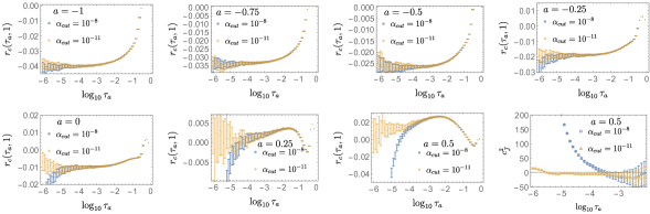
Figure 11: NLO remainder functions for $\alpha_{\text{cut}}=10^{-11}$ (blue) and for $10^{-8}$ (yellow) at seven different values of $a$. The last plot shows prediction of 2-loop constant $c_{\tilde{J}}^{2}$ as a function of lower bound $\tau_{a}^{\text{low}}$ for $\alpha_{\text{cut}}=10^{-11}$ and for $10^{-8}$.

Fig. 12 shows the cutoff effect in the gluon channel as a function of $\tau_{a}^{\text{low}}$ with $\log_{10}\tau_{a}^{\text{high}}=-1.4+0.4\,(1+a)$ held fixed. Similar to the quark channel, larger $a$ values tend to suffer from greater cutoff effect $c_{\tilde{J}}^{2}$. Using the results, our fit regions are selected to avoid the cutoff effect as described in main body of the paper.

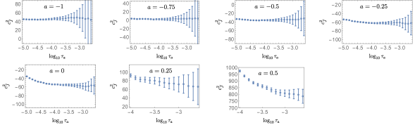
Figure 12: two-loop constant $c_{\tilde{J}}^{2}$ as a function of lower bound $\tau_{a}^{\text{low}}$ with fixed-upper bound $\log_{10}\tau_{a}^{\text{high}}=-1.4+0.4\,(1+a)$ at $\alpha_{\text{cut}}=10^{-8}$

References

- (1) ATLAS collaboration, Observation of a new particle in the search for the Standard Model Higgs boson with the ATLAS detector at the LHC, Phys. Lett. B 716 (2012) 1 [1207.7214].
- (2) CMS collaboration, Observation of a New Boson at a Mass of 125 GeV with the CMS Experiment at the LHC, Phys. Lett. B 716 (2012) 30 [1207.7235].
- (3) CMS collaboration, Observation of H production, Phys. Rev. Lett. 120 (2018) 231801 [1804.02610].
- (4) ATLAS collaboration, Observation of Higgs boson production in association with a top quark pair at the LHC with the ATLAS detector, Phys. Lett. B 784 (2018) 173 [1806.00425].
- (5) ATLAS collaboration, Observation of decays and production with the ATLAS detector, Phys. Lett. B 786 (2018) 59 [1808.08238].
- (6) CMS collaboration, Observation of Higgs boson decay to bottom quarks, Phys. Rev. Lett. 121 (2018) 121801 [1808.08242].
- (7) CMS collaboration, Sensitivity projections for Higgs boson properties measurements at the HL-LHC, .
- (8) J. Gao, Differentiating the production mechanisms of the Higgs-like resonance using inclusive observables at hadron colliders, JHEP 02 (2014) 094 [1308.5453].
- (9) Y. Soreq, H.X. Zhu and J. Zupan, Light quark Yukawa couplings from Higgs kinematics, JHEP 12 (2016) 045 [1606.09621].
- (10) F. Bishara, U. Haisch, P.F. Monni and E. Re, Constraining Light-Quark Yukawa Couplings from Higgs Distributions, Phys. Rev. Lett. 118 (2017) 121801 [1606.09253].
- (11) G.T. Bodwin, F. Petriello, S. Stoynev and M. Velasco, Higgs boson decays to quarkonia and the coupling, Phys. Rev. D 88 (2013) 053003 [1306.5770].
- (12) A.L. Kagan, G. Perez, F. Petriello, Y. Soreq, S. Stoynev and J. Zupan, Exclusive Window onto Higgs Yukawa Couplings, Phys. Rev. Lett. 114 (2015) 101802 [1406.1722].
- (13) Y. Zhou, Constraining the Higgs boson coupling to light quarks in the HZZ final states, Phys. Rev. D 93 (2016) 013019 [1505.06369].
- (14) M. König and M. Neubert, Exclusive Radiative Higgs Decays as Probes of Light-Quark Yukawa Couplings, JHEP 08 (2015) 012 [1505.03870].
- (15) G. Perez, Y. Soreq, E. Stamou and K. Tobioka, Prospects for measuring the Higgs boson coupling to light quarks, Phys. Rev. D 93 (2016) 013001 [1505.06689].
- (16) A.S. Chisholm, S. Kuttimalai, K. Nikolopoulos and M. Spannowsky, Measuring rare and exclusive Higgs boson decays into light resonances, Eur. Phys. J. C 76 (2016) 501 [1606.09177].
- (17) F. Goertz, A. Papaefstathiou, L.L. Yang and J. Zurita, Higgs Boson self-coupling measurements using ratios of cross sections, JHEP 06 (2013) 016 [1301.3492].
- (18) CMS collaboration, Combination of searches for Higgs boson pair production in proton-proton collisions at 13 TeV, Phys. Rev. Lett. 122 (2019) 121803 [1811.09689].
- (19) CMS collaboration, Prospects for HH measurements at the HL-LHC, .
- (20) ATLAS collaboration, Search for Higgs boson pair production in the final state with 13 TeV collision data collected by the ATLAS experiment, JHEP 11 (2018) 040 [1807.04873].
- (21) T. Behnke, J.E. Brau, B. Foster, J. Fuster, M. Harrison, J.M. Paterson et al., eds., The International Linear Collider Technical Design Report - Volume 1: Executive Summary, 1306.6327.
- (22) CEPC Study Group collaboration, CEPC Conceptual Design Report: Volume 2 - Physics & Detector, 1811.10545.
- (23) P. Lebrun, L. Linssen, A. Lucaci-Timoce, D. Schulte, F. Simon, S. Stapnes et al., The CLIC Programme: Towards a Staged e+e- Linear Collider Exploring the Terascale : CLIC Conceptual Design Report, 1209.2543.
- (24) TLEP Design Study Working Group collaboration, First Look at the Physics Case of TLEP, JHEP 01 (2014) 164 [1308.6176].
- (25) J. Gao, Probing light-quark Yukawa couplings via hadronic event shapes at lepton colliders, JHEP 01 (2018) 038 [1608.01746].
- (26) J. Gao, Y. Gong, W.-L. Ju and L.L. Yang, Thrust distribution in Higgs decays at the next-to-leading order and beyond, JHEP 03 (2019) 030 [1901.02253].
- (27) M.-X. Luo, V. Shtabovenko, T.-Z. Yang and H.X. Zhu, Analytic Next-To-Leading Order Calculation of Energy-Energy Correlation in Gluon-Initiated Higgs Decays, JHEP 06 (2019) 037 [1903.07277].
- (28) J. Gao, V. Shtabovenko and T.-Z. Yang, Energy-energy correlation in hadronic Higgs decays: analytic results and phenomenology at NLO, JHEP 02 (2021) 210 [2012.14188].
- (29) G. Coloretti, A. Gehrmann-De Ridder and C.T. Preuss, QCD predictions for event-shape distributions in hadronic Higgs decays, JHEP 06 (2022) 009 [2202.07333].
- (30) A. Gehrmann-De Ridder, C.T. Preuss and C. Williams, Four-jet event shapes in hadronic Higgs decays, 2310.09354.
- (31) J. Mo, F.J. Tackmann and W.J. Waalewijn, A case study of quark-gluon discrimination at NNLL’ in comparison to parton showers, Eur. Phys. J. C 77 (2017) 770 [1708.00867].
- (32) S. Alioli, A. Broggio, A. Gavardi, S. Kallweit, M.A. Lim, R. Nagar et al., Resummed predictions for hadronic Higgs boson decays, JHEP 04 (2021) 254 [2009.13533].
- (33) W.-L. Ju, Y. Xu, L.L. Yang and B. Zhou, Thrust distribution in Higgs decays up to the fifth logarithmic order, Phys. Rev. D 107 (2023) 114034 [2301.04294].
- (34) B. Yan and C. Lee, Probing light quark Yukawa couplings through jet angularities in Higgs boson decay, in The 2022 International Workshop on the High Energy Circular Electron Positron Collider.
- (35) C.W. Bauer, S. Fleming and M.E. Luke, Summing Sudakov logarithms in B — X(s gamma) in effective field theory, Phys. Rev. D 63 (2000) 014006 [hep-ph/0005275].
- (36) C.W. Bauer, S. Fleming, D. Pirjol and I.W. Stewart, An Effective field theory for collinear and soft gluons: Heavy to light decays, Phys. Rev. D 63 (2001) 114020 [hep-ph/0011336].
- (37) C.W. Bauer and I.W. Stewart, Invariant operators in collinear effective theory, Phys. Lett. B 516 (2001) 134 [hep-ph/0107001].
- (38) C.W. Bauer, D. Pirjol and I.W. Stewart, Soft collinear factorization in effective field theory, Phys. Rev. D 65 (2002) 054022 [hep-ph/0109045].
- (39) C.W. Bauer, S. Fleming, D. Pirjol, I.Z. Rothstein and I.W. Stewart, Hard scattering factorization from effective field theory, Phys. Rev. D 66 (2002) 014017 [hep-ph/0202088].
- (40) C.W. Bauer, S.P. Fleming, C. Lee and G.F. Sterman, Factorization of e+e- Event Shape Distributions with Hadronic Final States in Soft Collinear Effective Theory, Phys. Rev. D 78 (2008) 034027 [0801.4569].
- (41) A. Hornig, C. Lee and G. Ovanesyan, Effective Predictions of Event Shapes: Factorized, Resummed, and Gapped Angularity Distributions, JHEP 05 (2009) 122 [0901.3780].
- (42) G. Bell, A. Hornig, C. Lee and J. Talbert, angularity distributions at NNLL′ accuracy, JHEP 01 (2019) 147 [1808.07867].
- (43) J. Zhu, D. Kang and T. Maji, Angularity in DIS at next-to-next-to-leading log accuracy, JHEP 11 (2021) 026 [2106.14429].
- (44) A. Budhraja, A. Jain and M. Procura, One-loop angularity distributions with recoil using Soft-Collinear Effective Theory, JHEP 08 (2019) 144 [1903.11087].
- (45) A.J. Larkoski, D. Neill and J. Thaler, Jet Shapes with the Broadening Axis, JHEP 04 (2014) 017 [1401.2158].
- (46) P. Bijl, S. Niedenzu and W.J. Waalewijn, Probing factorization violation with vector angularities, 2307.02521.
- (47) M. Beneke, A.P. Chapovsky, M. Diehl and T. Feldmann, Soft collinear effective theory and heavy to light currents beyond leading power, Nucl. Phys. B 643 (2002) 431 [hep-ph/0206152].
- (48) M. Beneke and T. Feldmann, Multipole expanded soft collinear effective theory with nonAbelian gauge symmetry, Phys. Lett. B 553 (2003) 267 [hep-ph/0211358].
- (49) T. Inami, T. Kubota and Y. Okada, Effective Gauge Theory and the Effect of Heavy Quarks in Higgs Boson Decays, Z. Phys. C 18 (1983) 69.
- (50) A. Djouadi, J. Kalinowski and P.M. Zerwas, Higgs radiation off top quarks in high-energy e+ e- colliders, Z. Phys. C 54 (1992) 255.
- (51) K.G. Chetyrkin, B.A. Kniehl and M. Steinhauser, Hadronic Higgs decay to order alpha-s**4, Phys. Rev. Lett. 79 (1997) 353 [hep-ph/9705240].
- (52) K.G. Chetyrkin, B.A. Kniehl and M. Steinhauser, Decoupling relations to O (alpha-s**3) and their connection to low-energy theorems, Nucl. Phys. B 510 (1998) 61 [hep-ph/9708255].
- (53) K.G. Chetyrkin, J.H. Kuhn and C. Sturm, QCD decoupling at four loops, Nucl. Phys. B 744 (2006) 121 [hep-ph/0512060].
- (54) P.A. Baikov, K.G. Chetyrkin and J.H. Kühn, Five-Loop Running of the QCD coupling constant, Phys. Rev. Lett. 118 (2017) 082002 [1606.08659].
- (55) M.D. Schwartz, Resummation and NLO matching of event shapes with effective field theory, Phys. Rev. D 77 (2008) 014026 [0709.2709].
- (56) T. Becher and M.D. Schwartz, A precise determination of from LEP thrust data using effective field theory, JHEP 07 (2008) 034 [0803.0342].
- (57) T. Gehrmann, E.W.N. Glover, T. Huber, N. Ikizlerli and C. Studerus, Calculation of the quark and gluon form factors to three loops in QCD, JHEP 06 (2010) 094 [1004.3653].
- (58) G. Bell, R. Rahn and J. Talbert, Generic dijet soft functions at two-loop order: uncorrelated emissions, JHEP 09 (2020) 015 [2004.08396].
- (59) K.M. Brune, Automation of jet function calculations in Soft-Collinear Effective theory, Ph.D. thesis, Siegen U., 2022. 10.25819/ubsi/10228.
- (60) Z. Ligeti, I.W. Stewart and F.J. Tackmann, Treating the b quark distribution function with reliable uncertainties, Phys. Rev. D 78 (2008) 114014 [0807.1926].
- (61) R. Abbate, M. Fickinger, A.H. Hoang, V. Mateu and I.W. Stewart, Thrust at with Power Corrections and a Precision Global Fit for , Phys. Rev. D 83 (2011) 074021 [1006.3080].
- (62) T. Becher, M. Neubert and B.D. Pecjak, Factorization and Momentum-Space Resummation in Deep-Inelastic Scattering, JHEP 01 (2007) 076 [hep-ph/0607228].
- (63) T. Becher and M. Neubert, Threshold resummation in momentum space from effective field theory, Phys. Rev. Lett. 97 (2006) 082001 [hep-ph/0605050].
- (64) A.H. Hoang and S. Kluth, Hemisphere Soft Function at O(alpha(s)**2) for Dijet Production in e+ e- Annihilation, 0806.3852.
- (65) OpenLoops 2 collaboration, OpenLoops 2, Eur. Phys. J. C 79 (2019) 866 [1907.13071].
- (66) A. van Hameren, OneLOop: For the evaluation of one-loop scalar functions, Comput. Phys. Commun. 182 (2011) 2427 [1007.4716].
- (67) G. Ossola, C.G. Papadopoulos and R. Pittau, CutTools: A Program implementing the OPP reduction method to compute one-loop amplitudes, JHEP 03 (2008) 042 [0711.3596].
- (68) T. Hahn, CUBA: A Library for multidimensional numerical integration, Comput. Phys. Commun. 168 (2005) 78 [hep-ph/0404043].
- (69) S.G. Gorishnii, A.L. Kataev, S.A. Larin and L.R. Surguladze, Corrected Three Loop QCD Correction to the Correlator of the Quark Scalar Currents and (Tot) ( Hadrons), Mod. Phys. Lett. A 5 (1990) 2703.
- (70) A.N. Tikhonov, On the solution of ill-posed problems and the method of regularization, in Doklady akademii nauk, vol. 151, pp. 501–504, Russian Academy of Sciences, 1963.
- (71) Z. Nagy and Z. Trocsanyi, Next-to-leading order calculation of four jet observables in electron positron annihilation, Phys. Rev. D 59 (1999) 014020 [hep-ph/9806317].
- (72) Z. Nagy, Next-to-leading order calculation of three jet observables in hadron hadron collision, Phys. Rev. D 68 (2003) 094002 [hep-ph/0307268].
- (73) T. Gleisberg and F. Krauss, Automating dipole subtraction for QCD NLO calculations, Eur. Phys. J. C 53 (2008) 501 [0709.2881].
- (74) C.F. Berger, C. Marcantonini, I.W. Stewart, F.J. Tackmann and W.J. Waalewijn, Higgs Production with a Central Jet Veto at NNLL+NNLO, JHEP 04 (2011) 092 [1012.4480].
- (75) D. Kang, C. Lee and I.W. Stewart, Using 1-Jettiness to Measure 2 Jets in DIS 3 Ways, Phys. Rev. D 88 (2013) 054004 [1303.6952].
- (76) D. Kang, C. Lee and I.W. Stewart, Analytic calculation of 1-jettiness in DIS at , JHEP 11 (2014) 132 [1407.6706].
- (77) C. Lee and G.F. Sterman, Momentum Flow Correlations from Event Shapes: Factorized Soft Gluons and Soft-Collinear Effective Theory, Phys. Rev. D 75 (2007) 014022 [hep-ph/0611061].
- (78) A.H. Hoang and I.W. Stewart, Designing gapped soft functions for jet production, Phys. Lett. B 660 (2008) 483 [0709.3519].
- (79) C.F. Berger and G.F. Sterman, Scaling rule for nonperturbative radiation in a class of event shapes, JHEP 09 (2003) 058 [hep-ph/0307394].
- (80) R. Abbate, M. Fickinger, A.H. Hoang, V. Mateu and I.W. Stewart, Precision Thrust Cumulant Moments at LL, Phys. Rev. D 86 (2012) 094002 [1204.5746].
- (81) Y.-T. Chien, D. Kang, K. Lee and Y. Makris, Subtracted Cumulants: Mitigating Large Background in Jet Substructure, Phys. Rev. D 100 (2019) 074030 [1812.06977].
- (82) D. Kang, Y. Makris and T. Mehen, From Underlying Event Sensitive To Insensitive: Factorization and Resummation, JHEP 09 (2018) 055 [1803.04413].
- (83) R. Abdul Khalek et al., Science Requirements and Detector Concepts for the Electron-Ion Collider: EIC Yellow Report, 2103.05419.
- (84) Z. Chu, Y. Wang, J.-H. Ee, J. Chen and D. Kang, I-jettiness with jet axis at O(s) in deep inelastic scattering, JHEP 06 (2022) 111 [2202.08040].
- (85) G. Bell, R. Rahn and J. Talbert, Two-loop anomalous dimensions of generic dijet soft functions, Nucl. Phys. B 936 (2018) 520 [1805.12414].
- (86) S.D. Ellis, C.K. Vermilion, J.R. Walsh, A. Hornig and C. Lee, Jet Shapes and Jet Algorithms in SCET, JHEP 11 (2010) 101 [1001.0014].
- (87) A. Hornig, Y. Makris and T. Mehen, Jet Shapes in Dijet Events at the LHC in SCET, JHEP 04 (2016) 097 [1601.01319].
- (88) S. Moch, J.A.M. Vermaseren and A. Vogt, The Three loop splitting functions in QCD: The Nonsinglet case, Nucl. Phys. B 688 (2004) 101 [hep-ph/0403192].
- (89) G.P. Korchemsky and A.V. Radyushkin, Renormalization of the Wilson Loops Beyond the Leading Order, Nucl. Phys. B 283 (1987) 342.
- (90) S.A. Larin and J.A.M. Vermaseren, The Three loop QCD Beta function and anomalous dimensions, Phys. Lett. B 303 (1993) 334 [hep-ph/9302208].
- (91) O.V. Tarasov, A.A. Vladimirov and A.Y. Zharkov, The Gell-Mann-Low Function of QCD in the Three Loop Approximation, Phys. Lett. B 93 (1980) 429.