On the relationship between stochastic turnpike and dissipativity notions

Abstract

In this paper, we introduce and study different dissipativity notions and different turnpike properties for discrete-time stochastic nonlinear optimal control problems. The proposed stochastic dissipativity notions extend the classic notion of Jan C. Willems to $L^{r}$ random variables and to probability measures. Our stochastic turnpike properties range from a formulation for random variables via turnpike phenomena in probability and in probability measures to the turnpike property for the moments. Moreover, we investigate how different metrics (such as Wasserstein or Lévy-Prokhorov) can be leveraged in the analysis. Our results are built upon stationarity concepts in distribution and in random variables and on the formulation of the stochastic optimal control problem as a finite-horizon Markov decision process. We investigate how the proposed dissipativity notions connect to the various stochastic turnpike properties and we work out the link between these two different forms of dissipativity.

Stochastic optimal control, stochastic systems, dissipativity, stability of nonlinear systems

1 Introduction

Dissipativity and strict dissipativity as introduced by Willems [32, 33] and the so-called turnpike property—first observed by Ramsey [25] and von Neumann [31]—are important tools for analyzing the qualitative properties of optimally controlled systems. While dissipativity states that a system cannot contain more energy than supplied from the outside, the turnpike property describes the phenomenon that optimal and near-optimal trajectories spend most of the time near a particular solution, which in the simplest case is an optimal steady state of the system. The connection of these properties to model predictive and receding horizon control [5, 6, 9, 10, 3, 2, 22, 17] has fueled a lot of recent research activities, but the topic also received attention in fields such as optimal control with partial differential equations [14, 15, 29, 34], shape optimization [19], or mean field games [24].

For deterministic optimal control problems, the relation between dissipativity and the turnpike property are well understood. Loosely speaking, under mild condition strict dissipativity implies the turnpike property while the converse is true under somewhat more restrictive conditions [7, 11, 12]. For stochastic optimal control problems, this relation is so far only very little explored. One of the challenges that arises here is to identify the appropriate probabilistic objects for which such an analysis can be carried out. Two possible such objects are the distributions and the moments of the solutions of the optimally controlled system, and most of the current work about stochastic turnpike properties are using one of these, e.g. [18, 20, 28]. The approach via distributions is also closely related to a probability measure based definition of dissipativity of stochastic optimal control problems in [8]. While this approach can be used to characterize the qualitative behavior of the probability distribution and moments of optimal solutions, it does not allow to obtain pathwise information, since two random variables with the same distribution are indistinguishable through the lens of moments and measures. However, recent numerical results in [23] show that pathwise turnpike properties can be expected in concrete examples.

Motivated by this observation, the authors recently introduced an alternative dissipativity notion for discrete-time linear-quadratic (LQ) optimal control problems, using the representation of the stochastic states and controls via random variables, see [26, 27]. It turns out that this notion can be used to analyze both the distributional and the pathwise behavior of the problem. Furthermore, we have shown that the stationary distribution in our approach is characterized by the same optimization problem as for the probability measure based approach, cf. [27, Remark 5.3]. Nevertheless, the exact connection between these two dissipativity notions is not yet clear and the available analysis is so far limited to LQ optimal control problems.

Thus, the contribution of this paper is twofold: we investigate the relationship between these two dissipativity concepts and we carry out a dissipativity and turnpike analysis for general discrete-time nonlinear stochastic optimal control problems. To this end, we introduce four types of turnpike properties—in $L^{r}$, pathwise in probability, in distribution, and for the moments—and show that they form a hierarchy. Crucially, the metric used for the distributions (e.g., Wasserstein or Lévy-Prokhorov) determine the details of the considered hierarchy. We furthermore investigate how the strict dissipativity concepts—for the random variable and for distributions—relate to each other and which of the four turnpike properties they imply. Figure 1, below, gives an overview of the implications we obtain. Compared to the LQ case, the proofs for the nonlinear case require a completely different way of reasoning, since the tools from LQ optimal control like the superposition principle and the Riccati equation are not available.

The remainder of the paper is structured as follows. Section 2 introduces the stochastic optimal control problems under consideration and the different forms of dissipativity and turnpike behavior that we study. Moreover, we define the stationarity concepts used later. In Section 3, we present the main results. We show which turnpike properties are induced by the different dissipativity notions and analyze the connection of these notions. Furthermore, we show that the stationary distribution needed in the strict dissipativity and turnpike formulations can be characterized by an optimality condition. The theoretical findings are illustrated by a nonlinear example in Section 4 while Section 5 concludes the paper.

2 Setting and definitions

Before presenting the main results of this paper in Section 3, we start by introducing the stochastic optimal control problems under consideration. Moreover, we define the different concepts of stochastic dissipativity and turnpike used for our investigations.

2.1 The stochastic optimal control problem

We consider discrete-time stochastic control systems described by a function

$$f:\mathcal{X}\times\mathcal{U}\times\mathcal{W}\rightarrow\mathcal{X},\quad(x,u,w)\mapsto f(x,u,w),$$

which is continuous in $(x,u)\in\mathcal{X}\times\mathcal{U}$ for almost all realizations $w\in\mathcal{W}$, where $\mathcal{X}$, $\mathcal{U}$, and $\mathcal{W}$ are separable Banach-spaces. The control system is then defined by the iteration

$$X(k+1)=f(X(k),U(k),W(k)),\quad X(0)=X_{0},$$ (1)

where $W(k)$ is independent of $X(k)$ and $U(k)$ and $(W(0),W(1),\ldots)$ is an i.i.d. sequence of random variables with distribution $\varrho_{W}$. In order to define the stochastic state and input spaces for the system, for a separable Banach-space $(\mathcal{X},\|\cdot\|_{\mathcal{X}})$ and a probability space $(\Omega,\mathcal{F},\mathbb{P})$, we denote by $L^{n}(\Omega,\mathcal{F},\mathbb{P};\mathcal{X})$ the space of $\mathcal{F}$-measurable random variables $X:\Omega\rightarrow\mathcal{X}$ with finite $n$-th moments equipped with the norm

$$\|X\|_{L^{n}}:=\mathbb{E}\left[\|X\|_{\mathcal{X}}^{n}\right]^{1/n}=\left(\int_{\Omega}\|X\|_{\mathcal{X}}^{n}~{}\mbox{d}\mathbb{P}\right)^{1/n}.$$

We assume $X(k)\in L^{n}(\Omega,\mathcal{F}_{k},\mathbb{P};\mathcal{X})$ and $U(k)\in L^{l}(\Omega,\mathcal{F}_{k},\mathbb{P};\mathcal{U})$, where $(\mathcal{F}_{k})_{k\in\mathbb{N}_{0}}$ is the smallest filtration such that $X$ is an adapted process, i.e.

$$\mathcal{F}_{k}=\sigma(X(0),\ldots,X(k))\subseteq\mathcal{F},\quad k\in\mathbb{N}_{0}.$$

This choice of the stochastic filtration induces a causality requirement, which ensures that the control action $U(k)$ at time $k$ only depends on the initial condition and on the sequence of past disturbances $(W(0),\ldots,W(k-1))$ but not on future events. We refer to [7, 18] for more details on stochastic filtrations. In addition to the filtration condition we impose constraints $(X,U)\in\mathbb{Y}\subseteq L^{n}(\Omega,\mathcal{F},\mathbb{P};\mathcal{X})\times L^{l}(\Omega,\mathcal{F},\mathbb{P};\mathcal{U})$ on the stochastic state $X$ and control $U$ which are assumed to be law-invariant, i.e., if $(X,U)\in\mathbb{Y}$ then $(Y,V)\in\mathbb{Y}$ also holds for all $(X,U)\sim(Y,V)$. Here $(X,U)\sim(Y,V)$ means that the pair $(X,U)$ has the same joint distribution as $(Y,V)$. Law-invariant constraints can be, for instance, chance constraints, constraints on single moments, or constraints associated to law-invariant risk measures like the value at risk. We define the sets

$$\begin{split}\mathbb{X}:=\{X\in&L^{n}(\Omega,\mathcal{F},\mathbb{P};\mathcal{X})\mid\\ &\exists U\in L^{n}(\Omega,\mathcal{F},\mathbb{P};\mathcal{U})~{}:~{}(X,U)\in\mathbb{Y}\}\phantom{.}\end{split}$$

and

$$\begin{split}\mathbb{U}:=\{U\in&L^{n}(\Omega,\mathcal{F},\mathbb{P};\mathcal{U})\mid\\ &\exists X\in L^{n}(\Omega,\mathcal{F},\mathbb{P};\mathcal{X})~{}:~{}(X,U)\in\mathbb{Y}\}.\end{split}$$

A control sequence $\mathbf{U}:=(U(0),\ldots,U(N-1))\in\mathbb{U}^{N}$ is called admissible for $X_{0}\in\mathbb{X}$ if $U(k)\in L^{l}(\Omega,\mathcal{F}_{k},\mathbb{P};\mathcal{U})$, $(X(k),U(k))\in\mathbb{Y}$ for all $k=0,\ldots,N-1$, and $X(N)\in\mathbb{X}$. In this case, the corresponding trajectory is also called admissible. The set of admissible control sequences is denoted by $\mathbb{U}^{N}(X_{0})$. Likewise, we define $\mathbb{U}^{\infty}(X_{0})$ as the set of all control sequences $\mathbf{U}\in\mathbb{U}^{\infty}$ with $U(k)\in L^{l}(\Omega,\mathcal{F}_{k},\mathbb{P};\mathcal{U})$ and $(X(k),U(k))\in\mathbb{Y}$ for all $k\in\mathbb{N}_{0}$. For technical simplicity, we assume that $\mathbb{X}$ is control invariant, i.e., that $\mathbb{U}^{\infty}(X_{0})\neq\emptyset$ for all $X_{0}\in\mathbb{X}$. For an initial value $X_{0}\in\mathbb{X}$, a control sequence $\mathbf{U}\in\mathbb{U}^{N}(X_{0})$, and a noise sequence $\mathbf{W}:=(W(0),\ldots,W(N-1))$ we denote the trajectories of (1) as $X_{\mathbf{U}}(k,X_{0},\mathbf{W})$ or short $X(k,\mathbf{W})$ if there is no ambiguity about $X_{0}$ and $\mathbf{U}$.

In order to extend the stochastic system (1) to a stochastic optimal control problem, we consider stage costs $\ell:\mathbb{Y}\rightarrow\mathbb{R}$, which are also assumed to be law-invariant, i.e., for any two pairs $(X,U)$ and $(Y,V)$ it holds that $\ell(X,U)=\ell(Y,V)$ if $(X,U)\sim(Y,V)$.

Then, in summary, the stochastic optimal control problem on horizon $N\in\mathbb{N}\cup\{\infty\}$ under consideration reads

$$\begin{split}\min_{\mathbf{U}\in\mathbb{U}^{N}(X_{0})}J_{N}(X_{0},\mathbf{U}):=&\sum_{k=0}^{N-1}\ell(X(k),U(k))\\ s.t.~{}X(k+1)&=f(X(k),U(k),W(k))\\ X(0)&=X_{0}.\end{split}$$ (2)

2.2 Markov policies and stationarity

In stochastic settings, the concept of an equilibrium of a deterministic system has to be extended to a more general stationarity concept. Hence, a structured analysis of stationary solutions to (1) is pivotal for our further developments. It is known, see ,e.g.  [26, 27], and in fact quite obvious that in general a pair of constant random variables $(X,U)\in L^{n}(\Omega,\mathcal{F},\mathbb{P};\mathcal{X})\times L^{l}(\Omega,\mathcal{F},\mathbb{P};\mathcal{U})$ is not a steady state of (1) if the system is subject to persistent excitation by the noise. A natural remedy here is to look for constant distributions rather than for constant solutions and this is the first form of stationarity we consider in this paper. However, as we want to analyze the behavior of the random variable $X(k)$ as an element of $L^{n}(\Omega,\mathcal{F},\mathbb{P};\mathcal{X})$ and also pathwise, looking at distributions alone does not provide sufficient information. Hence, in the work at hand we also replace the deterministic steady states by stationary processes $X(k)$ and $U(k)$, i.e., by solutions of (1) that vary with time $k$ but whose distributions are constant over time.

In order to formalize this, we first need to show that for obtaining optimal stationary solutions—or, in fact, general optimal solutions—we can restrict ourselves to control sequences that do not depend on $X(0),\ldots,X(k)$ but only on $X(k)$. To this end, we start with the following lemma, which directly follows from [16, Lemma 1.14] applied to the function

$$\hat{X}:\Omega\rightarrow\mathcal{X}^{k+1},\quad\hat{X}(\omega)=(X(0)(\omega),\ldots,X(k)(\omega)).$$

Lemma 2.1

A control process $U(\cdot)$ is adapted to the filtration $(\mathcal{F}_{k})_{k\in\mathbb{N}_{0}}$, i.e. $\sigma(U(k))\subseteq\mathcal{F}_{k}$, if and only if there is a measurable function $\pi_{k}:\mathcal{X}^{k+1}\rightarrow\mathcal{U},k\in\mathbb{N}_{0}$ such that

$$U(k)=\pi_{k}(X(0),\ldots,X(k)),\quad\mbox{for all }k\in\mathbb{N}_{0}.$$

Lemma 2.1 shows that we can equivalently look at sequences $\boldsymbol{\pi}=(\pi_{0},\pi_{1},\ldots)$ instead of adapted control processes $U(\cdot)$ under the assumed filtration condition. The functions $\pi_{k}$ are called feedback strategies or policies.

Since we demand that $U(k)\in L^{l}(\Omega,\mathcal{F}_{k},\mathbb{P};\mathcal{U})\subseteq L^{l}(\Omega,\mathcal{F},\mathbb{P};\mathcal{U})$, we have to ensure that

$$U(k)=\pi_{k}(X(0),\ldots,X(k))\in L^{l}(\Omega,\mathcal{F},\mathbb{P};\mathcal{U})$$

for all $k\in\mathbb{N}_{0}$ when switching to feedback strategies. Thus, we introduce the set $\Pi_{k}(\mathcal{X},\mathcal{U})$ given by

$$\begin{split}\Pi_{k}(\mathcal{X},\mathcal{U}):=\{\pi:\mathcal{X}^{k+1}\rightarrow\mathcal{U}\mid\pi\circ X\in L^{l}(\Omega,\mathcal{F},\mathbb{P};\mathcal{U})\qquad\\ \mbox{ for all }X\in(L^{n}(\Omega,\mathcal{F},\mathbb{P};\mathcal{X}))^{k+1}\}.\end{split}$$

Although we can now use feedback strategies instead of control processes, the problem that the admissible set depends on the time still remains, since $\Pi_{k}\subset\Pi_{k+1}$ holds for all $k\in\mathbb{N}_{0}$. However, the reformulation of the problem via policies now allows to prove that the solution of the optimal control problem (2) can always be characterized by a sequence of so-called Markov policies, i.e., policies $\boldsymbol{\pi}=(\pi_{0},\ldots,\pi_{N-1})$ with $\pi_{k}\in\Pi_{0}(\mathcal{X},\mathcal{U})$ for all $k=0,\ldots,N-1$. Here the name “Markov policy” for $\boldsymbol{\pi}$ refers to the fact that for $U(k)=\pi_{k}\circ X(k)$ the system (1) defines a Markov chain.

Theorem 2.2

Define the set of controls $\mathbb{F}^{N}(X_{0})\subseteq\mathbb{U}^{N}(X_{0})$ generated by Markov policies as

$$\begin{split}\mathbb{F}^{N}(X_{0}):=\{\mathbf{U}\in&\mathbb{U}^{N}(X_{0})\mid\exists\pi_{k}\in\Pi_{0}(\mathcal{X},\mathcal{U}):\\ &\qquad U(k)=\pi_{k}(X(k)),~{}k=0,\ldots,N\}.\end{split}$$

Then for all $N\in\mathbb{N}$ and $X_{0}\in\mathbb{X}$ it holds that

$$\min_{\mathbf{U}\in\mathbb{U}^{N}(X_{0})}J_{N}(X_{0},\mathbf{U})=\min_{\mathbf{U}\in\mathbb{F}^{N}(X_{0})}J_{N}(X_{0},\mathbf{U}).$$

The theorem above is a direct consequence of [1, Theorem 6.2], which is based on the fact that for any sequence of policies, there exists an equivalent sequence of Markov policies inducing the same joint distributions, and the law-invariance of the constraints. For more technical details on the proof we also refer to [4]. Theorem 2.2 shows that we can restrict the control sequences to the set $\mathbb{F}^{N}(X_{0})$ without losing any optimal solutions. This restriction has the advantage that we can replace the time dependent filtration condition by constraining the controls to Markov policies which only depend on the current state and not the whole history of the states. Markov policies greatly simplify the analysis of the optimally controlled system because we know that for a Markov strategy $\pi$, the system

$$X(k+1)=f(X(k),\pi(X(k)),W(k))$$

always defines a Markov chain. This directly implies that for every Markov policy $\pi$ there is a transition probability $p_{\pi}:\mathcal{X}\rightarrow\mathcal{P}(X)$ only depending on the distribution of the noise such that

$$\mathbb{P}(x(k+1)\in A|x(k)=y)=p_{\pi}(y,A)$$

for every $A\in\mathcal{B}(\mathcal{X})$, almost every $x\in\mathcal{X}$ and every $k\in\mathbb{N}$, see [21]. Thus, for $X_{k}\sim\varrho_{k}$ and any Markov policy $\pi\in\Pi_{0}(\mathcal{X},\mathcal{U})$ we can compute the distribution $\varrho_{k+1}$ of $X(k+1)$ using the transition operator given by

$$\varrho_{k+1}=\mathcal{T}(\pi,\varrho_{k})=\int_{\mathcal{X}}p_{\pi}(y,\pi(y))\varrho_{k}(dy).$$ (3)

Put differently, for a given policy $\pi$ the distribution $\varrho_{k+1}$ only depends on the distribution $\varrho_{k}$ but not on the particular form of $X(k)$ as a random variable. In turn, this implies that for a given Markov policy the forward propagation of the distribution of the state does also only depend on the current distribution. Hence,

$$f(X,\pi(X),W)\sim f(\widetilde{X},\pi(\widetilde{X}),W)$$

holds for all $\widetilde{X}\sim X$ and $W\sim\rho_{W}$ independent of the particular choice of $W$, $X$ and $\widetilde{X}$.

We want to use this properties in the remainder of the paper, thus, henceforth the optimal control problem under consideration reads

$$\begin{split}\min_{\mathbf{U}\in\mathbb{F}^{N}(X_{0})}J_{N}(X_{0},\mathbf{U}):=&\sum_{k=0}^{N-1}\ell(X(k),U(k))\\ s.t.~{}X(k+1)&=f(X(k),U(k),W(k))\\ X(0)&=X_{0},\end{split}$$ (4)

which is problem (2) restricted to the set of Markov policies. We emphasize again that the set of optimal solutions to (2) and (4) coincides, although (4) in general has a smaller set of feasible solutions, cf. Theorem 2.2.

Now we have all the technical prerequisites to introduce the two different concepts of stationarity for our stochastic system that we deal with in this paper. To this end, we define the set

$$\mathcal{P}_{n}(\mathcal{X}):=\left\{\mu\in\mathcal{P}(\mathcal{X})~{}\middle|~{}\int_{\mathcal{X}}\|x\|^{n}\mu(\mbox{d}x)<\infty\right\},$$

where $\mathcal{P}(\mathcal{X})$ denotes the set of all probability measures. It is directly clear that for every random variable $X\in L^{n}(\Omega,\mathcal{F},\mathbb{P};\mathcal{X})$ with $X\sim\varrho$ we have $\varrho\in\mathcal{P}_{n}(\mathcal{X})$ and, thus, the set $\mathcal{P}_{n}(\mathcal{X})$ has a natural connection to $L^{n}(\Omega,\mathcal{F},\mathbb{P};\mathcal{X})$. The next definition now formalizes stationarity in sense of distributions.

Definition 2.3 (Stationary policy and distribution)

A distribution-policy pair $(\varrho^{s}_{X},\pi^{s})$ with $\varrho^{s}_{X}\in\mathcal{P}_{n}(\mathcal{X})$ and $\pi^{s}\in\Pi_{0}(\mathcal{X},\mathcal{U})$ is called stationary for system (1) if for all $X\sim\varrho^{s}$ and disturbances $W\sim\varrho_{W}$ it holds that $f(X,\pi^{s}(X),W)\sim\varrho^{s}_{X}$.

Note that Definition 2.3 looks at a one step problem and, hence, only considers Markov policies $\pi^{s}\in\Pi_{0}(\mathcal{X},\mathcal{U})$. Therefore, as already mentioned above, from [21] we know that there is a transition operator $\mathcal{T}:\mathcal{P}_{n}(\mathcal{X})\times\Pi_{0}(\mathcal{X},\mathcal{U})\rightarrow\mathcal{P}_{n}(\mathcal{X})$ only depending on the distribution $\varrho_{W}$ of the noise which can be used to directly forward propagate the distribution of the states. This means that we can alternatively define the pair $(\varrho^{s}_{X},\pi^{s})$ as a steady state of the transition operator, i.e.

$$\mathcal{T}(\varrho_{X}^{s},\pi^{s})=\varrho_{X}^{s}.$$ (5)

This also shows that Markov policies are sufficient to characterize stationary distributions since we can iteratively reapply $\pi^{s}$ to keep the distribution constant for all $k\in\mathbb{N}_{0}$.

Since we also want to analyze the behavior of solutions in $L^{n}(\Omega,\mathcal{F},\mathbb{P};()\mathcal{X})$ as well as pathwise behaviors, we also make use of a stationarity concept of the random variables forming the solutions on the probability space $(\Omega,\mathcal{F},\mathbb{P})$. To this end, we define the subset $\Gamma(\mathcal{X})$ of $\mathcal{P}_{n}(\mathcal{X})$ by

$$\Gamma(\mathcal{X}):=\{\varrho\in\mathcal{P}_{n}(\mathcal{X})\mid\exists X\in L^{n}(\Omega,\mathcal{F},\mathbb{P};\mathcal{X}):~{}X\sim\varrho\}$$

and assume $(\varrho^{s}_{X},\pi^{s})\in\Gamma(\mathcal{X})\times\Pi_{0}(\mathcal{X},\mathcal{U})$ to ensure that we can always find a random variable $X\sim\varrho^{s}_{X}$. The following definition now extends the concept of stationarity from Definition 2.3 to a stochastic process.

Definition 2.4 (Stationary stochastic processes)

Given a sequence of disturbances $\mathbf{W}=(W(0),W(1),\ldots)$, the pair of the stochastic processes $(\mathbf{X}^{s},\mathbf{U}^{s})$ given by

$$X^{s}_{\mathbf{U}^{s}}(k+1,\mathbf{W})=f(X^{s}_{\mathbf{U}^{s}}(k,\mathbf{W}),U^{s}(k),W(k))$$

with $\mathbf{U}^{s}\in\mathbb{F}^{\infty}(X^{s}(0))$ is called stationary for system (1) if

$$\begin{split}X^{s}_{\mathbf{U}^{s}}(k&,U(k),\mathbf{W})\sim\varrho^{s}_{X},\quad U(k)\sim\varrho^{s}_{U},\\ &(X^{s}_{\mathbf{U}^{s}}(k,\mathbf{W}),U^{s}(k))\sim\varrho^{s}_{X,U}\end{split}$$

for all $k\in\mathbb{N}_{0}$.

For any stationary stochastic process $(\mathbf{X}^{s},\mathbf{U}^{s})$ in the sense of Definition 2.4 the corresponding distribution $\varrho^{s}_{X}$ is stationary in the sense of Definition 2.3, i.e. a steady state of the transition operator (5). At the first glance this is not fully obvious, because the $\pi_{k}$ defining $\mathbf{U}^{s}\in\mathbb{F}^{\infty}(X^{s}(0))$ in Definition 2.4 may depend on time while $\pi^{s}$ in Definition 2.3 does not. However, because of equation (3) each $\pi_{k}$ has the property required for $\pi^{s}$ in Definition 2.3.

Conversely, for any stationary distribution there exists a stationary stochastic process, as the following lemma shows.

Lemma 2.5

Given a noise sequence $\mathbf{W}$ and a stationary feedback $\pi^{s}\in\Pi_{0}(\mathcal{X},\mathcal{U})$ with stationary distribution $\varrho_{X}^{s}\in\Gamma(\mathcal{X})$ such that $(X^{s},\pi^{s}(X^{s}))\in\mathbb{Y}$ for $X^{s}\sim\varrho^{s}_{X}$. Then for any $X_{\mathbf{U}^{s}}^{s}(0,\mathbf{W})\sim\varrho_{X}^{s}$ the pair $(\mathbf{X}^{s},\mathbf{U}^{s})$ given by

$$\begin{split}X_{\mathbf{U}^{s}}^{s}(k+1,\mathbf{W})&=f(X_{\mathbf{U}^{s}}^{s}(k,\mathbf{W}),U^{s}(k),W(k)),\\ U^{s}(k)&=\pi^{s}(X_{\mathbf{U}^{s}}^{s}(k,\mathbf{W}))\end{split}$$ (6)

is stationary for system (1).

Proof 2.1.

We can prove the first part by induction. Since $\varrho_{X}^{s}\in\Gamma(\mathcal{X})$ holds, the existence of a random variable $X_{0}\sim\varrho_{X}^{s}$ is ensured and we can set $X_{\mathbf{U}^{s}}^{s}(0,\mathbf{W})=X_{0}\sim\varrho_{X}^{s}$. Now assume that $X_{\mathbf{U}^{s}}^{s}(k,\mathbf{W})\sim\varrho_{X}^{s}$. Then we know that we can compute the distribution of $X_{\mathbf{U}^{s}}^{s}(k+1,\mathbf{W})$ by using the transition operator $\mathcal{T}$ since $f(X_{\mathbf{U}^{s}}^{s}(k,\mathbf{W}),U^{s}(k),W(k))$ defines a Markov chain for $U(k)=\pi^{s}(X_{\mathbf{U}^{s}}^{s}(k,\mathbf{W}))$. Thus, we get $X_{\mathbf{U}^{s}}^{s}(k+1,\mathbf{W})\sim\varrho_{X}^{s}$ because $\varrho_{X}^{s}$ is a steady state of the transition operator, which shows the staionaryity condition for $\mathbf{X}^{s}$. The stationarity condition on the distribution of $\mathbf{U}^{s}$ and joint distribution directly follows, because for a fixed Markov policy $\pi^{s}$, these two distributions are completely determined by the distribution $\varrho_{X}^{s}$ of the state.

Lemma 2.5 shows that Definition 2.4 is a natural extension of the stationarity concepts defined by the transition operator (5) to stochastic processes. The main difference between the stationarity in distribution usually used in the context of Markov decision processes and Definition 2.4 is that we impose the additional condition that the state process representing the stationary distribution follows the evolution of the stochastic system (1).

2.3 Dissipativity and strict dissipativity

The goal of this paper is to define (strict) dissipativity notions for nonlinear stochastic optimal control problems that allow to conclude a wide range of stochastic turnpike properties. The next two definitions provide these notions. The first one deals with the distributional behavior of the problem, while the second one is formulated for the random variables defining the solution process, such that we can gain information about the realization paths of the solutions. We denote by $P_{X}:\mathcal{B}(\mathcal{X})\rightarrow[0,1]\in\mathcal{P}_{n}(\mathcal{X})$ the push forward measure of the random variable $X\in L^{n}(\Omega,\mathcal{F},\mathbb{P};\mathcal{X})$ which characterizes its distribution and is defined by

$$P_{X}(A):=P(X^{-1}(A))\quad\mbox{for all}\quad A\in\mathcal{B}(\mathcal{X}).$$

Note that for a stationary process with distribution $\varrho_{X}^{s}$ we have $P_{X^{s}_{\mathbf{U}^{s}}(k,\mathbf{W})}=\varrho_{X}^{s}$ for all $k\in\mathbb{N}_{0}$. For a Markov strategy $\pi\in\Pi_{0}(\mathcal{X},\mathcal{U})$ we abbreviate the push forward measure of the subsequent state $X^{+}:=f(X,\pi(X),W)$ as $P_{X^{+}}$, since this measure does not depend on the exact representation of $W$.

Definition 6 (Distributional dissipativity).

Given a stationary feedback $\pi^{s}$ and a stationary distribution $\varrho_{X}^{s}$, we call the stochastic optimal control problem (4) strictly distributionally dissipative at $\varrho_{X}^{s}$, if there exists a storage function $\Lambda:\mathcal{P}(\mathcal{X})\rightarrow\mathbb{R}$ bounded from below, a metric $d_{D}$ on the space $\mathcal{P}_{n}(\mathcal{X})$, and a function $\alpha\in\mathcal{K}_{\infty}$ such that

$$\begin{split}\ell(X,\pi(X))-\ell(X^{s},\pi^{s}(X^{s}))+\Lambda(&P_{X})-\Lambda(P_{X^{+}})\\ &\geq\alpha(d_{D}(P_{X},\varrho^{s}_{X}))\end{split}$$ (7)

holds for all $(X,\pi(X))\in\mathbb{Y}$ and $X^{s}\sim\varrho^{s}_{X}$. The system is called distributionally dissipative, if inequality (7) holds with $\alpha\equiv 0$.

Since our stage costs and constraints are law-invariant, we can define $\hat{\ell}(\varrho,\pi):=\ell(X,\pi(X))$ for $X\sim\varrho$ and also consider the optimal control problem in probability measures, leading to the finite-horizon Markov decision problem

$$\begin{split}\min_{\boldsymbol{\pi}\in\mathbb{S}^{N}(\varrho_{0})}\hat{J}_{N}(\rho_{0},&\boldsymbol{\pi}):=\sum_{k=0}^{N-1}\hat{\ell}(\varrho_{k},\pi_{k})\\ s.t.~{}\varrho_{k+1}&=\mathcal{T}(\varrho_{k},\pi_{k}),~{}\varrho_{0}=\rho_{0}\end{split}$$ (8)

with

$$\begin{split}&\mathbb{S}^{N}(\varrho_{0}):=\{\boldsymbol{\pi}\in\Pi_{0}(\mathcal{X},\mathcal{U})^{N}\mid\\ &\quad\mathbf{U}=(\pi_{0}(X(0)),\ldots,\pi_{N-1}(X(N-1)))\in\mathbb{F}^{N}(X_{0}\sim\rho_{0})\}\end{split}$$

for some initial distribution $\rho_{0}\in P_{\mathbb{X}}:=\{\varrho\in\Gamma(\mathcal{X})\mid X\in\mathbb{X}\mbox{ for }X\sim\varrho\}$. This problem yields the same optimal strategies as problem (4) for $\varrho_{0}=P_{X_{0}}$. Since in Definition 6 we only consider Markov policies, the strict dissipation inequality (7) can thus be written as

$$\hat{\ell}(\varrho_{k},\pi)-\hat{\ell}(\varrho_{X}^{s},\pi^{s})+\Lambda(\varrho_{k})-\Lambda(\varrho_{k+1})\geq\alpha(d_{D}(\varrho_{k},\varrho^{s})),$$

which is the dissipativity notion based on probability measures introduced in [8], except that here we use a metric on probability measures instead of a dissimilarity measure. For the purpose of this paper, Definition 6 simplifies the transition between the distributional and the random variable perspective. This is important since next we also propose a dissipativity notion formulated in random variables, which takes the paths of the stochastic processes into account formalized in the following definition. Here and in the following, we use that for a stationary process $(\mathbf{X}^{s},\mathbf{U}^{s})$ due to the law-invariance of $\ell$ the value $\ell(X^{s}_{\mathbf{U}^{s}}(k,\mathbf{W}),U^{s}(k))$ is independent of $k$. We denote this value by $\ell(\mathbf{X}^{s},\mathbf{U}^{s})$.

Definition 7 ($L^{r}$ dissipativity in random variables).

Consider a pair of stationary stochastic processes $(\mathbf{X}^{s},\mathbf{U}^{s})$ for a given noise sequence $\mathbf{W}=(W(0),W(1),\ldots)$ according to Definition 2.4. Then we call the stochastic optimal control problem (4) strictly dissipative in $L^{r}$ at $X^{s}$, if there exists a storage function $\lambda:\mathbb{N}_{0}\times L^{n}(\Omega,\mathcal{F},\mathbb{P};\mathcal{X})\rightarrow\mathbb{R}$ bounded from below and a function $\alpha\in\mathcal{K}_{\infty}$ such that

$$\begin{split}&\ell(X(k,\mathbf{W}),U(k))-\ell(\mathbf{X}^{s},\mathbf{U}^{s})\\ &\qquad\quad+\lambda(k,X(k,\mathbf{W}))-\lambda(k+1,X(k+1,\mathbf{W}))\\ &\geq\alpha(\mathbb{E}\left[\|X(k,\mathbf{W})-X^{s}(k,\mathbf{W})\|_{\mathcal{X}}^{r}\right])\\ &\qquad\quad=\alpha(\|X(k,\mathbf{W})-X^{s}(k,\mathbf{W})\|_{L^{r}}^{r})\end{split}$$ (9)

holds for all $k\in\mathbb{N}_{0}$, $X_{0}\in\mathbb{X}$ and $\mathbf{U}\in\mathbb{F}^{\infty}(X_{0})$. The system is called $L^{r}$ dissipative if inequality (9) holds with $\alpha\equiv 0$.

Remark 8.

Definitions 2.4 and 7 can be easily extended to the non-Markovian setting by considering $\mathbb{U}^{N}(X_{0})$ instead of $\mathbb{F}^{N}(X_{0})$. However, in this case the storage function $\lambda$ from Definition 7 may implicitly depend on the whole history of the state process due to the underlying filtration. The reason for not considering this generalization is that such history-dependent $\lambda$ significantly complicate the analysis while not providing any benefit in our setting, because the optimal policies are Markov policies, as shown in Theorem 2.2. Moreover, for Definition 6 such a generalization is not possible, since for its formulation it is crucial that the information of the current distribution and feedback law is sufficient to compute the distribution of the subsequent state, which is only possible in the Markov setting using the transition operator (3).

2.4 Turnpike properties

At last we introduce four types of turnpike properties. Examining their connection with the dissipativity notions from Definition 6 and Definition 7 is the main purpose of this paper. We will do this in the next section. Note that in the following definition the metric $d_{D}$ used for the probability measures in part 3) is arbitrary. However, some of our results will only hold for specific metrics, which we define in Definition 10.

Definition 9 (Stochastic turnpike properties).

Consider a pair of stationary stochastic processes $(\mathbf{X}^{s},\mathbf{U}^{s})$ for a given noise sequence $\mathbf{W}=(W(0),W(1),\ldots)$ according to Definition 2.4 and set $\mathcal{N}=\{0,\ldots,N\}$. Then the stochastic optimal control problem is said to have the

1. $L^{r}$ turnpike property for some $r\leq n$ if for each $X_{0}\in\mathbb{X}$ there exists a $C_{a}>0$ and $\alpha_{1}\in\mathcal{K}_{\infty}$ such that for each $\delta>0$ and $N\in\mathbb{N}$, each control sequence $\mathbf{U}\in\mathbb{F}^{N}(X_{0})$ satisfying the condition $J_{N}(X_{0},\mathbf{U})\leq\delta+N\ell(\mathbf{X}^{s},\mathbf{U}^{s})$ and each $\varepsilon>0$ the value

   $$\begin{split}\mathcal{L}^{r}_{\varepsilon}:=\#\{&k\in\mathcal{N}\mid\\ &\mathbb{E}\left[\|X_{\mathbf{U}}(k,X_{0},\mathbf{W})-X^{s}(k,\mathbf{W})\|_{\mathcal{X}}^{r}\right]\leq\varepsilon\}\end{split}$$

   satisfies the inequality $\mathcal{L}^{r}_{\varepsilon}\geq N-(\delta+C_{a})/\alpha_{1}(\varepsilon)$.

2. pathwise-in-probability turnpike property if for each $X_{0}\in\mathbb{X}$ there exists a $C_{b}>0$ and $\alpha_{2}\in\mathcal{K}_{\infty}$ such that for each $\delta>0$ and $N\in\mathbb{N}$, each control sequence $\mathbf{U}\in\mathbb{F}^{N}(X_{0})$ satisfying the condition $J_{N}(X_{0},\mathbf{U})\leq\delta+N\ell(\mathbf{X}^{s},\mathbf{U}^{s})$ and each $\varepsilon>0$ the value

   $$\begin{split}&\mathcal{S}_{\varepsilon}:=\#\{k\in\mathcal{N}\mid\\ &\quad\mathbb{P}(\|X_{\mathbf{U}}(k,X_{0},\mathbf{W})-X^{s}(k,\mathbf{W})\|_{\mathcal{X}}\leq\varepsilon)\geq 1-\varepsilon\}\end{split}$$

   satisfies the inequality $\mathcal{S}_{\varepsilon}\geq N-(\delta+C_{b})/\alpha_{2}(\varepsilon)$.

3. distributional turnpike property if for each $X_{0}\in\mathbb{X}$ there exists a $C_{c}>0$, $\alpha_{3}\in\mathcal{K}_{\infty}$, and a metric $d_{D}$ on the space $\mathcal{P}_{n}(\mathcal{X})$ such that for each $\delta>0$ and $N\in\mathbb{N}$, each control sequence $\mathbf{U}\in\mathbb{F}^{N}(X_{0})$ satisfying the condition $J_{N}(X_{0},\mathbf{U})\leq\delta+N\ell(\mathbf{X}^{s},\mathbf{U}^{s})$ and each $\varepsilon>0$ the value

   $$\mathcal{D}_{\varepsilon}:=\#\left\{k\in\mathcal{N}\mid d_{D}(P_{X_{\mathbf{U}}(k,X_{0},\mathbf{W})},\varrho_{X}^{s})\leq\varepsilon\right\}$$

   satisfies the inequality $\mathcal{D}_{\varepsilon}\geq N-(\delta+C_{c})/\alpha_{3}(\varepsilon)$.

4. $r$-th moment turnpike property for some $r\leq n$ if for each $X_{0}\in\mathbb{X}$ there exists a $C_{d}>0$ and $\alpha_{4}\in\mathcal{K}_{\infty}$ such that for each $\delta>0$ and $N\in\mathbb{N}$, each control sequence $\mathbf{U}\in\mathbb{F}^{N}(X_{0})$ satisfying the condition $J_{N}(X_{0},\mathbf{U})\leq\delta+N\ell(\mathbf{X}^{s},\mathbf{U}^{s})$ and each $\varepsilon>0$ the value

   $$\begin{split}\mathcal{M}^{r}_{\varepsilon}:=\#\Big{\{}k\in\mathcal{N}\mid&\\ \Big{|}\mathbb{E}[\|&X_{\mathbf{U}}(k,X_{0},\mathbf{W})\|_{\mathcal{X}}^{r}]^{1/r}\\ &-\mathbb{E}[\|X^{s}(k,\mathbf{W})\|_{\mathcal{X}}^{r}]^{1/r}\Big{|}\leq\varepsilon\Big{\}}\end{split}$$

   satisfies the inequality $\mathcal{M}^{r}_{\varepsilon}\geq N-(\delta+C_{d})/\alpha_{4}(\varepsilon)$.

The turnpike behaviors given in the above definition state that those solutions to the stochastic optimal control problem (4), whose cost is close to that of the stationary process $(\mathbf{X}^{s},\mathbf{U}^{s})$, most of the time stay close to the stationary state process $\mathbf{X}^{s}$. The difference of the four turnpike behaviors 1)–4) in Definition 9 lies in the way how “close” is defined, i.e., in how we measure the distance between the solutions and the stationary state process.

In 1), we use the $L^{r}$-norm to define the neighborhood of the stationary process, while in 2), this neighborhood is defined in an appropriate in-probability sense for the solutions paths. The advantage of the in-probability definition is that it gives us a more descriptive interpretation of the pathwise solution behavior. It says that the probability that a single realization path does not have the turnpike property in the deterministic sense is low. This pathwise property of a realization is easy to be recognized in numerical simulations, without the need to know the stationary process, which is often difficult to calculate in applications. Specifically, in a preceding simulation study  [23] we have observed this pathwise property. In particular, for different initial conditions but identical disturbance realization paths, we observed that the middle part of finite-horizon optimal trajectories behaved very similar as all solutions were close to the pathwise-in-probability turnpike.

In part 3) of Definition 9, we focus on the underlying distributions of the random variables and say that a solution is near to $\mathbf{X}^{s}$ if their distributions are close to each other. Although the norm used for random variables is defined by the selection of the Banach-space $\mathcal{X}$, the norm used to measure the distance between distributions is still arbitrary in our setting, and several choices can lead to stronger or weaker statements about the behavior of the distributions. We specify two special cases of the turnpike and dissipativity in distribution.

Definition 10.

1. We say that the problem is (strictly) Wasserstein dissipative or has the Wasserstein turnpike property of order $r$, respectively, for some $r\leq n$ if Definition 6 or Definition 9(c), respectively, holds with $d_{D}$ being the Wasserstein distance of order $r$, i.e.,

   $$\begin{split}&d_{D}(P_{X},P_{Y})=d_{W_{r}}(P_{X},P_{Y})\\ &:=\inf\left\{\left(\mathbb{E}\left[\|\bar{X}-\bar{Y}\|_{\mathcal{X}}^{r}\right]\right)^{1/r}:~{}\bar{X}\sim P_{X},~{}\bar{Y}\sim P_{Y}\right\}.\end{split}$$

2. We say that the problem is (strictly) weakly distributionally dissipative or has the weak distributional turnpike property, respectively, if Definition 6 or Definition 9(c), respectively, holds with $d_{D}$ being the Lévy–Prokhorov metric, i.e.,

   $$\begin{split}d_{D}(&P_{X},P_{Y})=d_{LP}(P_{X},P_{Y})\\ &:=\inf\left\{d_{KF}(\bar{X},\bar{Y}):~{}\bar{X}\sim P_{X},~{}\bar{Y}\sim P_{Y}\right\},\end{split}$$

   where

   $$d_{KF}(X,Y):=\inf\left\{\varepsilon>0:\mathbb{P}\left(\|X-Y\|_{\mathcal{X}}>\varepsilon\right)\leq\varepsilon\right\}$$

   denotes the Ky-Fan-metric for two random variables $X,Y\in L^{n}(\Omega,\mathcal{F},\mathbb{P};\mathcal{X})$.

Here, the term “weak” in 2) refers to the fact that Lévy–Prokhorov metric can be used to characterize the weak convergence of measures.

The reason why these metrics are of particular interest to us will become clear when we compare them to the distance measures defining our turnpike properties regarding the random variables in Section 3.1. We can directly observe that the Wasserstein distance has a natural connection to $L^{r}$ norm while the Key-Fan metric is close to how we define the neighborhood of $\mathbf{X}^{s}$ for the pathwise-in-probability turnpike property. Finally, part 4) of Definition 9 formalizes that the $r$-th moments of the respective solutions are close to each other most of the time.

Remark 11.

In general it is possible that there is no control $U\in\mathbb{U}^{N}$ satisfying the performance bound $J_{N}(X_{0},\mathbf{U})\leq\delta+N\ell(\mathbf{X}^{s},\mathbf{U}^{s})$ demanded in Definition 9. Thus, to guarantee that there are such control sequences one has to impose suitable controllability or reachability assumptions on the stochastic system, similar to, e.g., the analysis in [10, Section 6] in the deterministic case. However, the technical details of such assumptions are beyond the scope of this paper.

Remark 12.

Since our definitions for turnpike and dissipativity are concerned with measuring the distance between state processes, one could also refer to these properties as state turnpike or state dissipativity, respectively. Another approach to gain additional information about the behavior of the control processes is to measure also the distances of the controls or policies in these definitions, which would lead to the definition of input-state turnpike and input-state dissipativity. This stronger properties for example hold in the standard stochastic linear-quadratic setting, cf. [26]. While we conjecture that one could extend the analysis in this paper to input-state turnpike properties using suitable regularity assumptions on the stochastic problem, in order to keep this paper concise we leave this as a question for future research.

3 Main results

In this section, we investigate the relationship between the different turnpike and dissipativity notions. Furthermore, we introduce the concept of optimal stationary solutions replacing the optimal deterministic steady state in stochastic systems.

3.1 Implications of strict $L^{r}$ dissipativity

We start with the following theorem, which shows that $L^{r}$ dissipativity implies the turnpike property in the same sense. Its proof uses the same arguments as in deterministic settings, cf. [10, 13].

Theorem 1.

Assume that the stochastic optimal control problem (4) is strictly $L^{r}$ dissipative. Then it has the $L^{s}$ turnpike property for all $s\leq r$.

Proof 3.1.

Set $C_{a}:=\lambda(0,X_{0})-M$ where $M\in\mathbb{R}$ is a uniform lower bound on $\lambda$ from Definition 7 for all $k\in\mathbb{N}_{0}$. Then for all $\mathbf{U}\in\mathbb{F}^{N}(X_{0})$ with $J_{N}(X_{0},\mathbf{U})<\delta+N\ell(\mathbf{X}^{s},\mathbf{U}^{s})$ we get

$$\begin{split}\tilde{J}_{N}(X_{0},\mathbf{U})=&\sum_{k=0}^{N-1}\ell(X(k,\mathbf{W}),U(k))-\ell(X^{s}(k,\mathbf{W}),U^{s}(k))\\ &\quad+\lambda(k,X(k,\mathbf{W}))-\lambda(k+1,X(k+1,\mathbf{W}))\\ =&\;J_{N}(X_{0},\mathbf{U})-N\ell(\mathbf{X}^{s},\mathbf{U}^{s})\\ &\quad+\lambda(0,X(0,\mathbf{W}))-\lambda(N,X(N,\mathbf{W}))\\ \leq&\;\delta+C_{a}.\end{split}$$ (10)

Now assume that $\mathcal{L}^{r}_{\varepsilon}<N-(\delta+C_{a})/\alpha_{1}(\varepsilon)$ with $\alpha_{1}=\alpha\in\mathcal{K}_{\infty}$ from Definition 7. Then there is a set $\mathcal{M}\subset\{0,\ldots,N-1\}$ of $N-\mathcal{L}^{r}_{\varepsilon}>(\delta+C_{a})/\alpha_{1}(\varepsilon)$ time instants such that $\mathbb{E}[\|X(k,\mathbf{W})-X^{s}(k,\mathbf{W})\|^{r}]\geq\varepsilon$ for all $k\in\mathcal{M}$. Using inequality (9) from Definition 7, this implies

$$\begin{split}\tilde{J}_{N}(X_{0},\mathbf{U})\geq&\sum_{k=0}^{N-1}\alpha_{1}\left(\mathbb{E}\big{[}\|X(k,\mathbf{W})-X^{s}(k,\mathbf{W})\|^{r}_{\mathcal{X}}\big{]}\right)\\ \geq&\sum_{k\in\mathcal{M}}\alpha_{1}\left(\mathbb{E}\big{[}\|X(k,\mathbf{W})-X^{s}(k,\mathbf{W})\|_{\mathcal{X}}^{r}\big{]}\right)\\ >&\dfrac{\delta+C_{a}}{\alpha_{1}(\varepsilon)}\alpha_{1}(\varepsilon)=\delta+C_{a}\end{split}$$

which contradicts (10) and, thus, proves the theorem for $s=r$. For $s<r$ the assertion follows directly from $\|X-Y\|_{L^{s}}\leq\|X-Y\|_{L^{r}}$ for all $X,Y\in L^{n}(\Omega,\mathcal{F},\mathbb{P};\mathcal{X})$.

The following theorem shows that one can also obtain the pathwise-in-probability turnpike property from the $L^{r}$ turnpike property and, thus, from the strict $L^{r}$ dissipativity.

Theorem 2.

Assume that the stochastic optimal control problem (4) has the $L^{r}$ turnpike property. Then it also has the pathwise-in-probability turnpike property.

Proof 3.2.

Using the Markov inequality, we get

$$\begin{split}\mathbb{P}\big{(}\|X(k,\mathbf{W})-&X^{s}(k,\mathbf{W})\|_{\mathcal{X}}\geq\varepsilon\big{)}\\ &\leq\dfrac{1}{\varepsilon^{r}}\mathbb{E}\left[\|X(k,\mathbf{W})-X^{s}(k,\mathbf{W})\|_{\mathcal{X}}^{r}\right].\end{split}$$ (11)

for all $r\in\mathbb{N}$. Further, by the definition of the turnpike $L^{r}$ property, cf. Definition 9, we know that for the $\mathcal{K}_{\infty}$ function $\alpha_{2}(\varepsilon):=\alpha_{1}(\varepsilon^{r+1})$ there are at least $N-(\delta+C_{a})/\alpha_{1}(\varepsilon^{r+1})$ time instants for which $\mathbb{E}[\|X(k,\mathbf{W})-X^{s}(k,\mathbf{W})\|^{r}]\leq\varepsilon^{r+1}$. Using equation (11), this gives

$$\mathbb{P}\left(\|X(k,\mathbf{W})-X^{s}(k,\mathbf{W})\|_{\mathcal{X}}\geq\varepsilon\right)\leq\varepsilon$$

for all these time instants which implies

$$\mathbb{P}\left(\|X(k,\mathbf{W})-X^{s}(k,\mathbf{W})\|_{\mathcal{X}}\leq\varepsilon\right)\geq 1-\varepsilon$$

and, thus, proves the claim with $C_{b}=C_{a}$.

Next, we show that pathwise turnpike in probability, in turn, implies a turnpike property for the underlying distributions. However, in general, this turnpike property cannot be concluded for an arbitrary metric on $\mathcal{P}_{n}(\mathcal{X})$. It does, however, hold for the Lévy–Prokhorov metric, as the following theorem shows.

Theorem 3.

If the stochastic optimal control problem (4) has the pathwise-in-probability turnpike property then it also has the weak distributional turnpike property in the sense of part 2) of Definition 10.

Proof 3.3.

Since the optimal control problem has the pathwise-in-probability turnpike property, we know by Definition 9 that there is an $\alpha_{2}\in\mathcal{K}_{\infty}$ such that there are at least $N-(\delta+C_{a})/\alpha_{2}(\varepsilon)$ time instants for which $\mathbb{P}\left(\|X(k,\mathbf{W})-X^{s}(k,\mathbf{W})\|_{\mathcal{X}}\leq\varepsilon\right)\geq 1-\varepsilon$ holds. Hence, it follows that

$$\begin{split}d_{KF}&(X(k,\mathbf{W}),X^{s}(k,\mathbf{W}))\\ &=\inf_{\epsilon>0}\left\{\mathbb{P}(\|X(k,\mathbf{W})-X^{s}(k,\mathbf{W})\|_{\mathcal{X}}>\epsilon)\leq\epsilon\right\}\leq\varepsilon\end{split}$$

holds for all these time instants, and thus, also

$$\begin{split}d_{LP}&(P_{X(k,\mathbf{W})},\varrho^{s}_{X})\\ &=\inf\{d_{KF}(X,Y):X\sim P_{X(k,\mathbf{W})},~{}Y\sim\varrho^{s}_{X}\}\leq\varepsilon,\end{split}$$

which proves the claim with $\alpha_{3}=\alpha_{2}\in\mathcal{K}_{\infty}$ and $C_{c}=C_{b}$.

Similar to stochastic convergence properties, the distributional turnpike property with respect to the Lévy–Prokhorov metric is a relatively weak property since, in general, we can not even conclude statements about the behavior of the moments from it. However, the Wasserstein metric is strong enough to let us make implications about the moments. Unfortunately, from the pathwise turnpike in probability, we cannot conclude the Wasserstein turnpike property, but this conclusion holds for the $L^{r}$ turnpike property, as the following theorem shows.

Theorem 4.

Assume the stochastic optimal control problem (4) has the $L^{r}$ turnpike property. Then it has the Wasserstein turnpike property of order $s$ for all $s\leq r$ in the sense of part 1) of Definition 10.

Proof 3.4.

Since $r\leq n$, we know that

$$\begin{split}\|X-&Y\|_{L^{r}}\geq\\ &\inf\left\{\left(\mathbb{E}\left[\|\bar{X}-\bar{Y}\|_{\mathcal{X}}^{r}\right]\right)^{1/r}:~{}\bar{X}\sim P_{X},~{}\bar{Y}\sim P_{Y}\right\}\\ &=d_{W_{r}}(P_{X},P_{Y})\geq 0\end{split}$$

holds for all $X,YL^{n}(\Omega,\mathcal{F},\mathbb{P};\mathcal{X})$. Thus,

$$\begin{split}\|X(k,\mathbf{W})-&X^{s}(k,\mathbf{W})\|_{L^{r}}^{r}\\ &=\mathbb{E}\left[\|X(k,\mathbf{W})-X^{s}(k,\mathbf{W})\|_{\mathcal{X}}^{r}\right]\leq\varepsilon\end{split}$$

implies that $d_{W_{r}}(P_{X(k,\mathbf{W})},\varrho^{s}_{X})\leq\varepsilon^{1/r}$ for all $\varepsilon>0$, which proves the claim for $s=r$ with $C_{c}=C_{a}$ and $\alpha_{3}(\varepsilon)=\alpha_{1}(\varepsilon^{1/r})\in\mathcal{K}_{\infty}$. For $s<r$ the assertion follows directly from $\|P_{X}-P_{Y}\|_{L_{s}}\leq\|P_{X}-P_{Y}\|_{L_{r}}$ for all$X,Y\in L^{n}(\Omega,\mathcal{F},\mathbb{P};\mathcal{X})$, cf. [30, Remark 6.6].

The next result shows that the Wasserstein turnpike property is indeed strong enough to imply turnpike of different moments.

Theorem 5.

Consider the stochastic optimal control problem (4) has the Wasserstein turnpike property. Then it has the $s$-th moment turnpike property for all $s\leq r$.

Proof 3.5.

Because $d_{W_{s}}(\cdot,\cdot)$ defines a metric on $\mathcal{P}_{n}(\mathcal{X})$, we get by the triangle inequality

$$d_{W_{s}}(P_{X},0)\leq d_{W_{s}}(P_{X},P_{Y})+d_{W_{s}}(P_{Y},0)$$

and

$$d_{W_{s}}(P_{Y},0)\leq d_{W_{s}}(P_{X},P_{Y})+d_{W_{s}}(P_{X},0)$$

which implies

$$\begin{split}|d_{W_{s}}(P_{X},0)-&d_{W_{s}}(P_{Y},0)|\\ &\leq d_{W_{s}}(P_{X},P_{Y})\leq d_{W_{r}}(P_{X},P_{Y})\end{split}$$

for all $X,Y\in L^{n}(\Omega,\mathcal{F},\mathbb{P};\mathcal{X})$ and $s\leq r\leq n$. Further, we have

$$\begin{split}d_{W_{s}}(P_{X},0)&=\inf\left\{\left(\mathbb{E}\left[\|\bar{X}-0\|_{\mathcal{X}}^{s}\right]\right)^{1/s}:~{}\bar{X}\sim P_{X}\right\}\\ &=\mathbb{E}\left[\|X\|_{\mathcal{X}}^{s}\right]^{1/s}\end{split}$$

and, thus, $d_{W_{r}}(P_{X(k,\mathbf{W})},\varrho_{X}^{s})\leq\varepsilon$ implies $|\mathbb{E}\left[\|X(k,\mathbf{W})\|_{\mathcal{X}}^{s}\right]^{1/s}-\mathbb{E}\left[\|X^{s}(k,\mathbf{W})\|_{\mathcal{X}}^{s}\right]^{1/s}|\leq\varepsilon$ which proves the theorem with $C_{d}=C_{c}$ and $\alpha_{4}=\alpha_{3}\in\mathcal{K}_{\infty}$.

3.2 Optimal stationary solutions

One of the key results in deterministic turnpike theory is that the steady state at which the turnpike property occurs—sometimes also referred to as the turnpike—is an optimal steady state. The generalization of this characterization to our setting is done in the following theorem. By using Lemma 2.5, it is sufficient to prove this statement for the stationary distribution in the sense of Definition 2.3, as Lemma 2.5 then implies that it also holds for Definition 2.4.

Theorem 6.

Let the stochastic optimal control problem (4) be distributionally dissipative at $(\varrho_{X}^{s},\pi^{s})$ with respect to a metric $d_{D}$. Then the stationary distribution $\varrho_{X}^{s}$ and the stationary feedback $\pi^{s}$ are an optimal solution to

$$\begin{split}&\min_{\pi,\varrho_{X}}\ell(X,U)\\ s.t.&~{}X\sim\varrho_{X},~{}U=\pi(X),~{}\\ &\varrho_{X}=\mathcal{T}(\varrho_{X},\pi),~{}(X,\pi(X))\in\mathbb{Y}.\end{split}$$ (12)

Moreover, if the problem is strictly dissipative in distribution, then the stationary distribution $\varrho_{X}^{s}\in\Gamma(\mathcal{X})$ is the unique (partial) solution of this problem, i.e., for every other solution $(\tilde{\varrho}_{X}^{s},\tilde{\pi}^{s})\in\Gamma(\mathcal{X})\times\Pi_{0}(\mathcal{X},\mathcal{U})$ we get $d_{D}(\varrho_{X}^{s},\tilde{\varrho}_{X}^{s})=0$.

Proof 3.6.

We prove the claim by contradiction. Assume distributional dissipativity and that there is a solution $(\tilde{\varrho}_{X}^{s},\tilde{\pi}^{s})\in\Gamma(\mathcal{X})\times\Pi_{0}(\mathcal{X},\mathcal{U})$ to problem (12) such that

$$\ell(\tilde{X}^{s},\tilde{\pi}^{s}(\tilde{X}^{s}))<\ell(X^{s},\pi^{s}(X^{s}))$$

for $\tilde{X}^{s}\sim\tilde{\varrho}_{X}^{s}$, $X^{s}\sim\varrho_{X}^{s}$. Then we get

$$\begin{split}&\ell(\tilde{X}^{s},\tilde{\pi}^{s}(\tilde{X}^{s}))-\ell(X^{s},\pi^{s}(X^{s}))+\Lambda(P_{\tilde{X}^{s}})-\Lambda(P_{(\tilde{X}^{s})^{+}})\\ &\quad=\ell(\tilde{X}^{s},\tilde{\pi}^{s}(\tilde{X}^{s}))-\ell(X^{s},\pi^{s}(X^{s}))<0,\end{split}$$ (13)

which contradicts (7) with $\alpha\equiv 0$ and, thus, the dissipativity of the optimal control problem. Here, we used that $P_{\tilde{X}^{s}}=P_{(\tilde{X}^{s})^{+}}$ for $\tilde{X}^{s}\sim\tilde{\varrho}_{X}^{s}$ due to the stationarity condition.

Now consider that the problem is strictly distributionally dissipative and $\ell(\tilde{X}^{s},\tilde{\pi}^{s}(\tilde{X}^{s}))=\ell(X^{s},\pi^{s}(X^{s}))$, but $d_{D}(\varrho_{X}^{s},\tilde{\varrho}_{X}^{s})>0$. Then we get by the definition of strict distributional dissipativity that there is a function $\alpha\in\mathcal{K}_{\infty}$ such that

$$\begin{split}0=&\ell(\tilde{X}^{s},\tilde{\pi}^{s}(\tilde{X}^{s}))-\ell(X^{s},\pi^{s}(X^{s}))\\ &+\Lambda(P_{\tilde{X}^{s}})-\Lambda(P_{(\tilde{X}^{s})^{+}})\\ \geq&\alpha(d_{D}(\varrho_{X}^{s},\tilde{\varrho}_{X}^{s})),\end{split}$$

which is again a contradiction since $\alpha(d_{D}(\varrho_{X}^{s},\tilde{\varrho}_{X}^{s}))>0$ for $d_{D}(\varrho_{X}^{s},\tilde{\varrho}_{X}^{s})>0$.

Theorem 6 shows how we can uniquely characterize an optimal stationary distribution similar to the deterministic setting. Although Theorem 6 considers strict distributional dissipativity, the same statement also holds in the case of strict $L^{r}$ dissipativity. We could show this by slightly modifying the proof of Theorem 6 as in [27, Theorem 5.3], which proves the statement in a linear-quadratic setting. However, we will choose another direction and conclude this fact from more general results on the relation of the two different (strict) dissipativity notions in random variables and in distribution (cf. Definitions 6 and 7). These results provide an interesting contribution in their own right.

3.3 Relation between (strict) dissipativity concepts

We start this section by proving that strict $L^{r}$ dissipativity implies strict distributional dissipativity. To this end, we use the following proposition, a variant of [12, Proposition 3.3] based on [32, Theorem 1] in our stochastic setting.

Proposition 7 (Available storage in distribution).

Let $\pi^{s}$ be a stationary feedback of system (1) with stationary distribution $\varrho_{X}^{s}$ such that $(X^{s},\pi^{s}(X^{s}))\in\mathbb{Y}$ for $X^{s}\sim\varrho^{s}_{X}$. Then there exists $\alpha\in\mathcal{K}_{\infty}$ (or $\alpha\equiv 0$, respectively) with

$$\begin{split}&\Lambda(P_{X_{0}}):=\sup_{\underset{\boldsymbol{\pi}\in\mathbb{S}^{N}(P_{X_{0}})}{N\in\mathbb{N}_{0}}}\sum_{k=0}^{N-1}-\Big{(}\hat{\ell}(P_{X(k)},\pi_{k})-\hat{\ell}(\varrho^{s}_{X},\pi^{s})\\ &\qquad\qquad\qquad\qquad\qquad\qquad-\alpha(d_{D}(P_{X(k)},\varrho_{X}^{s}))\Big{)}<\infty\end{split}$$ (14)

for all $P_{X_{0}}\in P_{\mathbb{X}}$ if and only if the stochastic optimal control problem (4) is strictly distributionally dissipative (or distributionally dissipative, respectively) with respect to the metric $d_{D}$. In this case, inequality (9) holds with $\Lambda$ and $\alpha$ from (14) and $\Lambda$ is called the available storage.

Proof 3.7.

Consider the Markov decision process (8). Then the statement follows directly by [12, Proposition 3.3], which proves the claim since distributional dissipativity of the probability measure based problem (8) and the stochastic optimal control problem (4) are equivalent.

Now, we can prove that strict $L^{r}$ dissipativity implies strict distributional dissipativity by showing that the function $\Lambda$ from (14) is bounded.

Theorem 8.

Assume the stochastic optimal control problem (4) is strictly $L^{r}$ dissipative. Then it is also strictly weakly distributionally dissipative and strictly Wasserstein dissipative of order $s$ for all $s\leq r$.

Proof 3.8.

Let $d_{D}(\cdot,\cdot)=d_{W_{s}}(\cdot,\cdot)$. From Definition 7 we know that there is a function $\hat{\alpha}\in\mathcal{K}_{\infty}$ such that

$$\begin{split}&\ell(X(k,\mathbf{W}),U(k))-\ell(\mathbf{X}^{s},\mathbf{U}^{s})\\ &\qquad\quad+\lambda(k,X(k,\mathbf{W}))-\lambda(k+1,X(k+1,\mathbf{W}))\\ &\geq\hat{\alpha}(\|X(k,\mathbf{W})-X^{s}(k,\mathbf{W})\|_{L^{r}}^{r})\\ &\qquad\quad=\alpha(\|X(k,\mathbf{W})-X^{s}(k,\mathbf{W})\|_{L^{r}})\end{split}$$

for $\alpha(z)=\hat{\alpha}(z^{r})\in\mathcal{K}_{\infty}$. Now let $M$ be a uniform lower bound on $\lambda$. Then for $(\varrho_{X}^{s},\pi^{s})\sim(\mathbf{X}^{s},\mathbf{U}^{s})$ we get

$$\begin{split}\sup_{\underset{\boldsymbol{\pi}\in\mathbb{S}^{N}(P_{X_{0}})}{N\in\mathbb{N}_{0}}}\sum_{k=0}^{N-1}-\Big{(}\hat{\ell}(P_{X(k)},\pi_{k})&-\hat{\ell}(\varrho^{s}_{X},\pi^{s})\\ -\alpha(&d_{D}(P_{X(k)},\varrho_{X}^{s}))\Big{)}\\ =\sup_{\underset{\mathbf{U}\in\mathbb{F}^{N}(X_{0})}{N\in\mathbb{N}_{0}}}\sum_{k=0}^{N-1}-\Big{(}\ell(X(k,\mathbf{W}),U(k))&-\ell(\mathbf{X}^{s},\mathbf{U}^{s})\\ -\alpha(&d_{D}(P_{X(k)},P_{X^{s}(k)}))\Big{)}\end{split}$$

and thus

$$\begin{split}\sup_{\underset{\boldsymbol{\pi}\in\mathbb{S}^{N}(P_{X_{0}})}{N\in\mathbb{N}_{0}}}\sum_{k=0}^{N-1}-\Big{(}\hat{\ell}(P_{X(k)},\pi_{k})&-\hat{\ell}(\varrho^{s}_{X},\pi^{s})\\ -\alpha(&d_{D}(P_{X(k)},\varrho_{X}^{s}))\Big{)}\\ \leq\sup_{\underset{\mathbf{U}\in\mathbb{F}^{N}(X_{0})}{N\in\mathbb{N}_{0}}}\sum_{k=0}^{N-1}-\Big{(}\ell(X(k,\mathbf{W}),U(k))&-\ell(\mathbf{X}^{s},\mathbf{U}^{s})\\ -\alpha(\|X(k,\mathbf{W}&)-X^{s}(k,\mathbf{W})\|_{L^{r}})\Big{)}\\ \leq\sup_{N\in\mathbb{N}_{0},\mathbf{U}\in\mathbb{F}^{N}(X_{0})}\sum_{k=0}^{N-1}\Big{(}\lambda(k,X(k,\mathbf{W}))&\\ -\lambda(k+1,&X(k+1,\mathbf{W}))\Big{)}\\ \leq\lambda(0,X_{0})-M<\infty.\qquad\qquad\qquad&\end{split}$$ (15)

for all $P_{X_{0}}\in P_{\mathbb{X}}$ and noise sequences $\mathbf{W}$. Thus, the assertion for strict Wasserstein dissipativity follows by Proposition 7. The assertion for strict weak distributional dissipativity follows analogously, since inequality above also holds for $d_{D}(\cdot,\cdot)=d_{LP}(\cdot,\cdot)$.

It is easy to see that Theorem 8 also holds for non-strict (meaning “not necessarily strict”) dissipativity. Indeed, for dissipativity the converse is is also true, as the following lemma shows.

Lemma 9.

The stochastic optimal control problem (4) is $L^{r}$ dissipative if and only if it is distributionally dissipative.

Proof 3.9.

“$\Rightarrow$” Assume that the stochastic optimal control problem (4) is strict $L^{r}$ dissipative. Then the inequality (15) also holds with $\alpha\equiv 0$ which implies distributional dissiptivity by Proposition 7.
“$\Leftarrow$” Assume that the stochastic optimal control problem is distributionally dissipative, i.e.,

$$\begin{split}0\leq&\ell(X,\pi(X))-\ell(X^{s},\pi^{s}(X^{s}))+\Lambda(P_{X})-\Lambda(P_{X^{+}})\end{split}$$ (16)

holds for all for all $(X,\pi(X))\in\mathbb{Y}$ and $X^{s}\sim\varrho^{s}_{X}$. Further, we know that $P_{X(k,\mathbf{W})}=P_{X(k)}$ for all noise sequences $\mathbf{W}$ and for $(\mathbf{X}^{s},\mathbf{U}^{s})\sim(\varrho_{X}^{s},\pi^{s})$ the identity $\ell(X^{s},\pi^{s}(X^{s}))=\ell(\mathbf{X}^{s},\mathbf{U}^{s})$ holds for $X^{s}\sim\varrho^{s}_{X}$. Thus, inequality (16) directly implies

$$\begin{split}0\leq\;&\ell(X(k,\mathbf{W}),U(k))-\ell(\mathbf{X}^{s},\mathbf{U}^{s})\\ &+\lambda(k,X(k,\mathbf{W}))-\lambda(k+1,X(k+1,\mathbf{W}))\end{split}$$

with $\lambda(k,X(k,\mathbf{W}))=\Lambda(P_{X(k,\mathbf{W})})$ for all $k\in\mathbb{N}_{0}$ and $(X(k,\mathbf{W}),U(k))\in\mathbb{Y}$ with $U(k)\in L^{l}(\Omega,\mathcal{F},\mathbb{P};\mathcal{U})$ and $U(k)=\pi(X(k))$ for some $\pi\in\Pi_{0}(\mathcal{X},\mathcal{U})$, which implies $L^{r}$ dissipativity.

The reason why the equivalence of the two dissipativity concepts in the sense of Lemma 9 holds is that for dissipativity the metric used to measure the distance between the random variables has no impact on the dissipation inequalities (7) and (9) since $\alpha\equiv 0$. However, for strict dissipativity the inequalities do depend on these metrics and since we cannot bound the $L^{r}$-norm from above by a metric on the space of probability measures, Lemma 9 does not hold for strict dissipativity.

3.4 Implications of strict distributional dissipativity

Now that we know how to switch between the different settings, we conclude the presentation of our main results by the following theorem, which shows that strict distributional dissipativity implies distributional turnpike. Again, the proof uses the same arguments as in deterministic settings.

Theorem 10.

Assume that the stochastic optimal control problem (4) is strictly distributionally dissipative with respect to a metric $d_{D}$. Then it has the distributional turnpike property with respect to the same metric.

Proof 3.10.

Set $C_{c}:=\lambda(P_{X_{0}})-M$ where $M\in\mathbb{R}$ is a bound on $\Lambda$ from Definition 6. Then for $(\mathbf{X}^{s},\mathbf{U}^{s})\sim(\varrho^{s}_{X},\pi^{s})$ and all $\mathbf{U}\in\mathbb{F}^{N}(X_{0})$ with $J_{N}(X_{0},\mathbf{U})<\delta+N\ell(\mathbf{X}^{s},\mathbf{U}^{s})$ we get

$$\begin{split}\tilde{J}_{N}(X_{0},\mathbf{U})=&\sum_{k=0}^{N-1}\ell(X(k,\mathbf{W}),U(k))-\ell(X^{s}(k,\mathbf{W}),U^{s}(k))\\ &\qquad\qquad+\Lambda(P_{X(k)})-\Lambda(P_{X(k+1)})\\ =&J_{N}(X_{0},\mathbf{U})-N\ell(\mathbf{X}^{s},\mathbf{U}^{s})\\ &\qquad\qquad+\Lambda(P_{X_{0}})-\Lambda(P_{X(N)})\\ &\leq\delta+C_{c}.\end{split}$$ (17)

Now assume that $\mathcal{D}_{\varepsilon}<N-(\delta+C_{c})/\alpha_{3}(\varepsilon)$ with $\alpha_{3}=\alpha\in\mathcal{K}_{\infty}$ from Definition 6. Then there is a set $\mathcal{M}\subset\{0,\ldots,N-1\}$ of $N-\mathcal{D}_{\varepsilon}>(\delta+C_{c})/\alpha_{3}(\varepsilon)$ time instants such that $d_{D}(P_{X(k)},\varrho_{X}^{s})\geq\varepsilon$ for all $k\in\mathcal{M}$. Using inequality (7) from Definition 6, this implies

$$\begin{split}\tilde{J}_{N}(X_{0},\mathbf{U})\geq&\sum_{k=0}^{N-1}\alpha_{3}\left(d_{D}(P_{X(k)},\varrho_{X}^{s})\right)\\ \geq&\sum_{k\in\mathcal{M}}\alpha_{3}\left(d_{D}(P_{X(k)},\varrho_{X}^{s})\right)\\ >&\dfrac{\delta+C_{c}}{\alpha_{3}(\varepsilon)}\alpha_{3}(\varepsilon)=\delta+C_{c}\end{split}$$

which contradicts (17) and, thus, proves the theorem.

Figure 1: Schematic sketch of the main results.

4 Example

In this section, we illustrate the theoretical results of this paper. For a linear-quadratic example illustrating many of the results in this paper we refer to [27]. Here we provide an example showing that strict dissipativity in $L^{r}$ can also hold for an optimal control problem with nonlinear dynamics and non-quadratic cost. To this end, consider the one-dimensional stochastic optimal control problem

$$\begin{split}&\min_{\mathbf{U}}J_{N}(X_{0},\mathbf{U})=\sum_{k=0}^{N-1}\mathbb{E}\left[(U(k)-X(k))^{4}\right]+\gamma\mathbb{E}\left[U(k)\right]^{2}\\ &\quad s.t.~{}X(k+1)=(U(k)-X(k))^{2}+W(k),~{}X(0)=X_{0}\\ &\qquad X(k)\in L^{4}(\Omega,\mathcal{F},\mathbb{P};\mathbb{R}),~{}U(k)\in L^{4}(\Omega,\mathcal{F}_{k},\mathbb{P};\mathbb{R})\\ \end{split}$$ (18)

with $\gamma\geq 0$, $W(k)\sim\varrho_{W}\in\mathcal{P}_{4}(\mathcal{X})$, $\mathbb{E}\left[W(k)\right]=0$, and the $W(k)$ are stochastically independent pairwise for all $k=0,\ldots,N$ and from $X_{0}$. Thus, problem (18) satisfies all assumptions of our setting.

Furthermore, it is easy to see that the pair $(\mathbf{X}^{s},\mathbf{U}^{s})$ given by

$$\begin{split}X^{s}(k+1,\mathbf{W})&=(U^{s}(k)-X^{s}(k,\mathbf{W}))^{2}+W(k)=W(k),\\ U^{s}(k)&=X^{s}(k,\mathbf{W})\end{split}$$ (19)

defines a stationary pair of stochastic processes for problem (18) with stationary distribution $\varrho_{X}^{s}=\varrho_{W}$. Moreover, we have $\ell(\mathbf{X}^{s},\mathbf{U}^{s})=0$ and for $\lambda(k,X(k))=\mathbb{E}\left[(X(k)-X^{s}(k))^{2}\right]$ we get

$$\begin{split}&\ell(X(k,\mathbf{W}),U(k))-\ell(\mathbf{X}^{s},\mathbf{U}^{s})\\ &\qquad\qquad+\lambda(k,X(k,\mathbf{W}))-\lambda(k+1,X(k+1,\mathbf{W}))\\ =&\mathbb{E}\left[(U(k)-X(k,\mathbf{W}))^{4}\right]\\ &\quad+\gamma\mathbb{E}\left[U(k)\right]^{2}+\mathbb{E}\left[(X(k,\mathbf{W})-X^{s}(k,\mathbf{W}))^{2}\right]\\ &\quad-\mathbb{E}\left[((U(k)-X(k,\mathbf{W})^{2}+W(k)-X^{s}(k+1,\mathbf{W}))^{2}\right]\\ =&\mathbb{E}\left[(U(k)-X(k,\mathbf{W}))^{4}\right]\\ &\quad+\gamma\mathbb{E}\left[U(k)\right]^{2}+\mathbb{E}\left[(X(k,\mathbf{W})-X^{s}(k,\mathbf{W}))^{2}\right]\\ &\quad-\mathbb{E}\left[(U(k)-X(k,\mathbf{W})^{2})^{2}\right]\\ =&\gamma\mathbb{E}\left[U(k)\right]^{2}+\mathbb{E}\left[(X(k,\mathbf{W})-X^{s}(k,\mathbf{W}))^{2}\right]\\ \geq&\|X(k,\mathbf{W})-X^{s}(k,\mathbf{W})\|_{L^{2}}^{2},\end{split}$$

which shows that problem (18) is strictly $L^{2}$ dissipative. Thus, we can conclude that the optimal control problem (18) is also strictly distributionally dissipative and exhibits the $L^{2}$, the pathwise-in-probability, the distributional turnpike property, and the turnpike property of the first two moments. While strict dissipativity holds for arbitrary distributions $\varrho_{W}$ subject to the considered conditions, for our numerical simulation we have chosen $\varrho_{W}$ to be a two-point distribution such that $W(k)=a:=0.5$ with probability $p_{a}=0.2$ and $W(k)=b:=-0.125$ with probability $p_{b}=0.8$, to facilitate the visualization of the numerical results. Figure 2 shows all possible realization paths subject to the considered noise of the optimal solutions for $X_{0}=7$, $\gamma=50$ and $N=3,5,10$ together with the stationary processes from (19), where we can clearly observe the turnpike property of these realization paths.

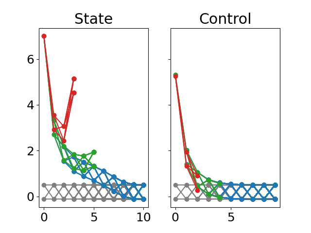
Figure 2: Evolution of all realization paths for the optimal trajectories (left) and controls (right) with $N=3$ in red, $N=5$ in green and $N=10$ in blue, as well as for the optimal stationary process (grey)

5 Conclusion

In this paper we have shown that strict $L^{r}$ dissipativity implies various types of turnpike properties for stochastic optimal control problems. We have proven, that $L^{r}$-based strict dissipativity also implies strict distributional dissipativity, which is equivalent to the dissipativity notion based on probability measures for stochastic problems introduced in [8]. We have seen that this dissipativity notion implies turnpike in the distributions of the optimal solutions. In the non-strict case, $L^{r}$ dissipativity and distributional dissipativity have turned out to be equivalent.

Some of the open questions that are not answered in this paper are: Under what conditions can one infer strict $L^{r}$ dissipativity from strict distributional dissipativity? Does the occurrence of the turnpike property in one of its various stochastic forms imply one or the other type of strict dissipativity? Can deterministic dissipativity results be used for the analysis of stochastically perturbed deterministic systems? Can one characterize the distributional robustness of the turnpike?

References

References

- [1] E. Altman. Constrained Markov Decision Processes. Routledge, 2021.
- [2] D. Angeli, R. Amrit, and J. B. Rawlings. On average performance and stability of economic model predictive control. IEEE transactions on automatic control, 57(7):1615–1626, 2011.
- [3] T. Breiten and L. Pfeiffer. On the turnpike property and the receding-horizon method for linear-quadratic optimal control problems. SIAM Journal on Control and Optimization, 58(2):1077–1102, 2020.
- [4] E. B. Dynkin and A. A. Yushkevich. Controlled Markov Processes, volume 235. Springer, 1979.
- [5] T. Faulwasser, L. Grüne, and M. A. Müller. Economic nonlinear model predictive control. Foundations and Trends® in Systems and Control, 5(1):1–98, 2018.
- [6] T. Faulwasser and L. Grüne. Turnpike properties in optimal control. In Numerical Control: Part A, pages 367–400. Elsevier, 2022.
- [7] T. Faulwasser, M. Korda, C. N. Jones, and D. Bonvin. On turnpike and dissipativity properties of continuous-time optimal control problems. Automatica, 81:297–304, jul 2017.
- [8] S. Gros and M. Zanon. Economic MPC of Markov decision processes: Dissipativity in undiscounted infinite-horizon optimal control. Automatica, 146:110602, dec 2022.
- [9] L. Grüne. Dissipativity and optimal control: examining the turnpike phenomenon. IEEE Control Syst. Mag., 42(2):74–87, 2022.
- [10] L. Grüne. Economic receding horizon control without terminal constraints. Automatica, 49(3):725–734, mar 2013.
- [11] L. Grüne and R. Guglielmi. Turnpike properties and strict dissipativity for discrete time linear quadratic optimal control problems. SIAM Journal on Control and Optimization, 56(2):1282–1302, jan 2018.
- [12] L. Grüne and M. A. Müller. On the relation between strict dissipativity and turnpike properties. Systems & Control Letters, 90:45–53, apr 2016.
- [13] L. Grüne, S. Pirkelmann, and M. Stieler. Strict dissipativity implies turnpike behavior for time-varying discrete time optimal control problems. In Lecture Notes in Economics and Mathematical Systems, pages 195–218. Springer International Publishing, 2018.
- [14] M. Gugat. On the turnpike property with interior decay for optimal control problems. Math. Control Signals Systems, 33(2):237–258, 2021.
- [15] M. Gugat and M. Herty. Turnpike properties of optimal boundary control problems with random linear hyperbolic systems. ESAIM Control Optim. Calc. Var., 29:Paper No. 55, 27, 2023.
- [16] O. Kallenberg. Foundations of Modern Probability. Springer International Publishing, 2021.
- [17] J. Köhler, M. A. Müller, and F. Allgöwer. On periodic dissipativity notions in economic model predictive control. IEEE Control Systems Letters, 2(3):501–506, 2018.
- [18] V. Kolokoltsov and W. Yang. Turnpike theorems for Markov games. Dynamic Games and Applications, 2(3):294–312, may 2012.
- [19] G. Lance, E. Trélat, and E. Zuazua. Shape turnpike for linear parabolic PDE models. Systems Control Lett., 142:104733, 9, 2020.
- [20] R. Marimon. Stochastic turnpike property and stationary equilibrium. Journal of Economic Theory, 47(2):282–306, apr 1989.
- [21] S. P. Meyn and R. L. Tweedie. Markov Chains and Stochastic Stability. Springer London, 1993.
- [22] M. A. Müller, D. Angeli, and F. Allgöwer. On necessity and robustness of dissipativity in economic model predictive control. IEEE Transactions on Automatic Control, 60(6):1671–1676, 2014.
- [23] R. Ou, M. H. Baumann, L. Grüne, and T. Faulwasser. A simulation study on turnpikes in stochastic LQ optimal control. IFAC-PapersOnLine, 54(3):516–521, 2021.
- [24] A. Porretta. On the turnpike property for mean field games. Minimax Theory Appl., 3(2):285–312, 2018.
- [25] F. P. Ramsey. A mathematical theory of saving. The Economic Journal, 38(152):543, dec 1928.
- [26] J. Schießl, R. Ou, T. Faulwasser, M. H. Baumann, and L. Grüne. Pathwise turnpike and dissipativity results for discrete-time stochastic linear-quadratic optimal control problems. Preprint arXiv:2303.15959, 2023.
- [27] J. Schießl, R. Ou, T. Faulwasser, M. H. Baumann, and L. Grüne. Turnpike and dissipativity in generalized discrete-time stochastic linear-quadratic optimal control. Preprint arXiv:2309.05422, 2023.
- [28] J. Sun, H. Wang, and J. Yong. Turnpike properties for stochastic linear-quadratic optimal control problems. Chinese Annals of Mathematics, Series B, 43(6):999–1022, nov 2022.
- [29] E. Trélat and C. Zhang. Integral and measure-turnpike properties for infinite-dimensional optimal control systems. Math. Control Signals Systems, 30(1):Art. 3, 34, 2018.
- [30] C. Villani. Optimal Transport: Old and New. Springer, 2009.
- [31] J. von Neumann. A model of general economic equilibrium. The Review of Economic Studies, 13(1):1, 1945.
- [32] J. C. Willems. Dissipative dynamical systems part I: General theory. Archive for rational mechanics and analysis, 45(5):321–351, 1972.
- [33] J. C. Willems. Dissipative dynamical systems part II: Linear systems with quadratic supply rates. Archive for rational mechanics and analysis, 45:352–393, 1972.
- [34] E. Zuazua. Large time control and turnpike properties for wave equations. Annual Reviews in Control, 44:199–210, 2017.