Gravitational waves from extreme-mass-ratio inspirals in the semiclassical gravity spacetime

Abstract

More recently, Fernandes Fernandes (2023) discovered analytic stationary and axially-symmetric black hole solutions within semiclassical gravity, driven by the trace anomaly. The study unveils some distinctive features of these solutions. In this paper, we compute the gravitational waves emitted from the extreme-mass-ratio inspiral (EMRI) around these quantum-corrected rotating black holes using the kludge approximate method. Firstly, we derive the orbital energy, angular momentum and fundamental frequencies for orbits on the equatorial plane. We find that, for the gravitational radiation described by quadrupole formulas, the contribution from the trace anomaly only appears at higher-order terms in the energy flux when compared with the standard Kerr case. Therefore, we can compute the EMRI waveforms from the quantum-corrected rotating black hole using the Kerr fluxes. We assess the differences between the EMRI waveforms from rotating black holes with and without the trace anomaly by calculating the dephasing and mismatch. Our results demonstrate that space-borne gravitational wave detectors can distinguish the EMRI waveform from the quantum-corrected black holes with a fractional coupling constant of $\sim 10^{-3}$ within one year observation. Finally, we compute the constraint on the coupling constant using the Fisher information matrix method and find that the potential constraint on the coupling constant by LISA can be within the error $\sim 10^{-4}$ in suitable scenarios.

I Introduction

The continuously rising occurrences of gravitational wave (GW) events resulting from the coalescence of compact binaries have been extensively reported Abbott et al. (2016, 2019, 2021a, 2021b). Various issues have been explored using the GW datasets, encompassing tests of General Relativity (GR) and its extensions Abbott et al. (2021c, 2022a), investigations into cosmic histories Abbott et al. (2023), examinations of dark matter Abbott et al. (2022b); Nagano et al. (2019), and more Abbott et al. (2020); Patricelli (2021). With advancements in current and future detector technologies in the realm of detectability, it becomes possible to explore novel astrophysical effects in the vicinity of dark and mysterious sources in the deep universe Cardoso and Pani (2019). This progress also enables investigations into the nature of classical and quantized horizons Cardoso and Pani (2017); Cardoso et al. (2016); Maggio et al. (2019); Arun et al. (2022). Particularly, according to the Kerr hypothesis in the context of GR Robinson (1975), these GW detections may help us to verify whether the massive compact objects are Kerr black holes (BHs) or not Barack and Cutler (2007); Cardoso and Gualtieri (2016); Zi et al. (2021). Besides, the presence of quantized signal of horizon is possible to be explored using the GW echoes observed by space-based GW detectors Cardoso and Pani (2017); Arun et al. (2022).

The no-hair theorem in the framework of GR supports that the BHs can be described by Kerr-Newmann (KN) solution without any charge Newman et al. (1965); Chrusciel et al. (2012). This, however, can be evaded in the alternatives of GR (see reviews Chrusciel et al. (2012); Berti et al. (2015); Barack et al. (2019)). In those extension theories, BHs can carry extra non-trivial scalar, vector or tenser hairs, which posses more complex multipolar structure compared with the stationary and axisymmetric Kerr BH. Additionally, after considering the exotic matter, the no-hair theorem can be circumvented, where the axisymmetry structure of spacetime is broken Liebling and Palenzuela (2023); Raposo and Pani (2020); Sanchis-Gual et al. (2021). The evitable cases of the no-hair theorem can result from the astrophysical environments, physical beyond GR and quantum corrections. Among the violation schemes, the semi-classical approach to GR, as an interesting and useful means to find BH solutions, includes the quantum effect of matter field and the classical spacetime geometry Hawking (1975). One popular trace anomaly method essentially is a one-loop quantum correction effect in the invariant classical theory, which breaks the conformal symmetry Capper and Duff (1974); Duff (1994). This could result in stress-energy tensor of quantum fields with non-trivial trace, which is related only with the curvature of spacetime, making it a feasible way to study the quantum phenomenon in the gravitational fields Anderson et al. (2007); Mottola and Vaulin (2006); Mottola (2017); Yang et al. (2022). More recently, analytic, stationary and axisymmetric spinning BH solutions have been obtained by considering the presence of the trace anomaly, which own the non-spherically symmetric event-horizon and violate the Kerr bound Fernandes (2023). Unlike the mass of Kerr BH that is independent of the other spatial coordinates, the quantum-corrected BH (QCBH) solution has a mass function, that is

$$\mathcal{M}(r,\theta)=\frac{2M}{1+\sqrt{1-\frac{8\alpha r\xi M}{\Sigma^{3}}}},$$ (1)

where $M$ is the ADM mass of the BH, $\Sigma=r^{2}+a^{2}\cos^{2}\theta$ and $\xi=r^{2}-3a^{2}\cos^{2}\theta$ with a spin parameter $a$, and $\alpha$ is the coupling constant of the trace anomaly. In the context of this new discovered QCBH, there are several works to study the different effects of the trace anomaly, including the validity of the weak cosmic censorship conjecture Jiang and Zhang (2023), the computation of BH shadows Zhang et al. (2023) and the study of the non-rotating and rotating cases with a cosmological constant Gurses and Tekin (2023). In this paper, we plan to study the detectability of the trace anomaly of the QCBH using the observations of the EMRIs, and put constraint on the coupling constant $\alpha$ with the future space-borne GW observatories, such as LISA Amaro-Seoane et al. (2017), TianQinLuo et al. (2016) and Taiji Ruan et al. (2020).

An EMRI is the dynamic process of inspiral, wherein a stellar-mass compact object (CO) with mass $\mu$ orbits around the massive black hole (MBH) with mass $M$ at the core of a galaxy. During this process, the orbits slowly dampen due to the radiated GWs until reaching the last stable orbit (LSO). The low frequency GW signal emitted from such binaries exactly lies in the $m\rm Hz$ band of LISA, which is expected to be one of the key target sources Berry et al. (2019); Berti et al. (2019). In addition, the EMRI systems carry a tiny mass ratios $\epsilon=\mu/M\in[10^{-7},10^{-4}]$, which implies that the CO accumulates $\mathcal{O}(1/\epsilon)\sim 10^{4}-10^{7}$ in the strong field regime until it is captured by the MBH. After matched filtering the phase in the LISA data stream with the waveform templates Gair et al. (2004); Amaro-Seoane et al. (2007), EMRI detections allow to accurately measure the parameters of sources or test the Kerr nature of the MBH Barack and Cutler (2007); Babak et al. (2017); Fan et al. (2020); Zi et al. (2021). From the point of view of astrophysics, it is possible to probe the astrophysical environment Kocsis et al. (2011); Barausse et al. (2014); Cardoso et al. (2022); Dai et al. (2023); Figueiredo et al. (2023); Zi and Li (2023a); Rahman et al. (2023a, b); Kumar et al. (2023). Besides, from the viewpoint of detecting the nature of horizons, there have been some works to study the differences of the presence or absence of horizon in the EMRI waveforms Sago and Tanaka (2021); Maggio et al. (2021); Zhang et al. (2021), which also considered several effects, such as tidal heating Datta and Bose (2019); Datta et al. (2020), tidal deformability Pani and Maselli (2019); De Luca et al. (2023); Zi and Li (2023b) and area quantization Agullo et al. (2021); Datta and Phukon (2021). Based on the above mentioned literature, it is feasible to probe the astrophysical effects near the horizon using the EMRI observations. Thus we intend to compute the EMRI waveform from the QCBHs and analyze the distinction of QCBHs from Kerr BHs by computing the dephasing and mismatch, then obtain the constraint on the deviation parameter $\alpha$ of QCBHs with Fisher information matrix (FIM) method.

This paper is organized as follows. In Sec. II, the calculation recipe of EMRI waveform in the spacetime of the QCBH is presented, which includes the review of the spacetime background and geodesics in II.1, the evolution method to compute EMRI inspiral trajectories in Sec. II.2, waveform formula and analysis method of GW data in Sec. II.3. We show the results of waveform comparison and the constraints using the EMRI observations of LISA in Sec. III. Finally, we give a brief summary in Sec. IV. The geometric units $G=c=1$ throughout this paper are utilized.

II Method

II.1 Background and geodesics

The stationary and axisymmetric BH solutions have been obtained by solving the semiclassical Einstein equations with the type-A trace anomaly. The solutions are called as QCBHs, whose line element is written as the following form in ingoing Kerr coordinates Fernandes (2023)

$$ds^{2}= -\left(1-\frac{2r\mathcal{M}(r,\theta)}{\Sigma}\right)(dv-a\sin^{2}\theta d\varphi)^{2}$$

$$+2(dv-a\sin^{2}\theta d\varphi)(dr-a\sin^{2}\theta d\varphi)$$ (2)

$$+\Sigma(d\theta^{2}+\sin^{2}\theta d\varphi^{2}).$$

Note that this metric is of the form of the one in the principled-parameterized approach that implements locality and regularity Eichhorn and Held (2021a, b). We would like to work in the more familiar Boyer-Lindquist coordinates. However, due to the fact that the spacetime is non-circular, the usual coordinate transformation between the the ingoing Kerr coordinates and the Boyer-Lindquist coordinates in the Kerr case cannot be applied here, since curvature singularities which lie on the horizon would be introduced. Refs. Eichhorn and Held (2021b); Delaporte et al. (2022) found the proper coordinate transformation that respects non-circularity is given by

$$t= v-\int dr\frac{r^{2}+a^{2}}{r^{2}+a^{2}-2\mathcal{M}(r,\theta)r},$$ (3)

$$\psi= \varphi-\int dr\frac{a}{r^{2}+a^{2}-2\mathcal{M}(r,\theta)r},$$ (4)

where the coordinates $t,r,\theta,\psi$ form the the standard coordinate system in Boyer-Lindquist form if $\mathcal{M}(r,\theta)$ is a constant. Then the metric of the QCBH can be written as

$$ds^{2}= g_{tt}dt^{2}+2g_{t\psi}dtd\psi+2g_{t\theta}dtd\theta+g_{rr}dr^{2}+g_{\theta\theta}d\theta^{2}$$

$$+2g_{\theta\psi}d\theta d\psi+g_{\psi\psi}d\psi^{2}$$

$$= -\left[1-\frac{2r\mathcal{M}}{\Sigma}\right]dt^{2}+\frac{\Sigma}{\Delta}dr^{2}-\frac{4ra\mathcal{M}\sin^{2}\theta}{\Sigma}dtd\psi$$

$$+\left[\frac{\Sigma}{\sin^{2}\theta}-\mathcal{M}_{2}^{2}-\sin^{2}\theta\mathcal{M}_{1}^{2}(r^{2}+a^{2})+\frac{2r\mathcal{M}}{\Sigma}\tilde{\mathcal{M}}^{2}\right]d\chi^{2}$$

$$-\left[(r^{2}+a^{2})\sin^{2}\theta+\frac{2\mathcal{M}ra^{2}\sin^{4}\theta}{\Sigma}\right]d\psi^{2}$$

$$+\left[\frac{4\mathcal{M}r\tilde{\mathcal{M}}}{\Sigma}-2\mathcal{M}_{2}\right]dtd\chi$$ (5)

$$-\left[\frac{4\mathcal{M}ra\tilde{\mathcal{M}}\sin^{2}\theta}{\Sigma}-2\sin^{2}\theta(r^{2}+a^{2})\mathcal{M}_{1}\right]d\chi d\psi,$$

with

$$\Delta=r^{2}-2\mathcal{M}r+a^{2},\quad\chi=\cos\theta,$$ (6)

$$\mathcal{M}_{1}(r,\chi)=\frac{d}{d\chi}\int dr\frac{a}{r^{2}+a^{2}-2\mathcal{M}(r,\theta)r},$$ (7)

$$\mathcal{M}_{2}(r,\chi)=\frac{d}{d\chi}\int dr\frac{r^{2}+a^{2}}{r^{2}+a^{2}-2\mathcal{M}(r,\theta)r},$$ (8)

and

$$\tilde{\mathcal{M}}(r,\chi)=\mathcal{M}_{1}(r,\chi)+\mathcal{M}_{2}(r,\chi).$$ (9)

One can see that above metric is far more complicated than the simple Kerr metric. However, one can find that if we restrict ourselves to the equatorial plane, the above metric would have a simple connection with the Kerr metric by replacing the mass in the Kerr metric with the mass function $(\ref{ADM:mass})$. When the parameter $\alpha=0$, the solution returns to the classical Kerr BH.

In this paper, we focus on the orbits and waveform of EMRIs, thus the timelike geodesics of the QCBH would be presented. Firstly, we introduce some basics about the geodesics. For a point particle, the Hamiltonian can be written as

$$\mathcal{H}=\frac{1}{2}g_{\mu\nu}p^{\mu}p^{\nu}=-\frac{1}{2}m^{2}$$ (10)

where $p^{\mu}$ and $m$ is the momentum and rest mass of the particle, respectively. Since the spacetime (II.1) are stationary and axisymmetric, the particle along the geodesic has two conserved quantities, i.e., the energy and $z$-component of the angular momentum,

$$\frac{E}{m}=-(g_{tt}\dot{t}+g_{t\psi}\dot{\psi}),~{}~{}~{}~{}~{}\frac{L_{z}}{m}=g_{t\psi}\dot{t}+g_{\psi\psi}\dot{\psi},$$ (11)

where the dot denotes differentiation with respect to proper time $\tau$. We can get two first-order decoupled differential equations about the $t$ and $\psi$ momenta in light of equations (11), the following form is written as

$$\dot{t}=\frac{Eg_{\psi\psi}+L_{z}g_{t\psi}}{m(g_{t\psi}^{2}-g_{tt}g_{\psi\psi})},~{}~{}~{}\dot{\psi}=\frac{Eg_{t\psi}+L_{z}g_{tt}}{m(g_{\psi\psi}g_{tt}-g^{2}_{t\psi})}.$$ (12)

In this paper we focus on the equatorial orbits, the coordinate $\theta$ becomes to $\theta=\pi$ and $\dot{\theta}=0$. According to the Eq. (10), we can obtain the equations of the $r$ and simply the Eqs. (12)

$$r^{2}\frac{dr}{d\tau} = \pm\sqrt{V_{r}}=\pm\sqrt{T^{2}-\Delta[m^{2}r^{2}+(L_{z}-aE)^{2}]},$$ (13)

$$r^{2}\frac{d\phi}{d\tau} = V_{\phi}=\frac{aT}{\Delta}+L_{z}-aE,$$ (14)

$$r^{2}\frac{dt}{d\tau} = V_{t}=\frac{(r^{2}+a^{2})T}{\Delta}+L_{z}-aE,$$ (15)

$$\theta(\tau) = \pi/2.$$ (16)

where $T=E(r^{2}+a^{2})-aL_{z}$. Since we will discuss the bound orbits, whose energy satisfies $0<E<1$. The bound orbits are described by the energy $E$, angular momentum $L_{z}$, semi-latus rectum $p$ and eccentricity $e$. For the equatorial eccentric orbit, there exists two turning points, that are the periastron $r_{p}$ and the apastron $r_{a}$,

$$r_{p}=\frac{p}{1+e},~{}~{}~{}r_{a}=\frac{p}{1-e}.$$ (17)

The radial potential $V_{r}$ satisfies $V_{r}(r_{a})=0$ and $V_{r}(r_{p})=0$, with this conditions, we can get the expressions $E$ and $x$ by defining $x=L_{z}-aE$. Since the function $\mathcal{M}$ dependents on $r$, the full expressions of $E$ and $x$ are lengthy to be to be listed even in the appendix, so we just put them in the ancillary Mathematica file. Using the parameters $p$ and $e$, the radial coordinate can be written as

$$r(\chi)=\frac{p}{1+e\cos\chi},$$ (18)

where $\chi$ is a monotonic parameter that varies from 0 to $2\pi$, it equals to 0 at $r=r_{p}$ and the parameter $\chi=\pi$ at $r=r_{a}$. According to the parameterization method (18), the geodesic equations can be transformed as

$$\frac{dr}{d\tau} = \frac{\sqrt{\mathcal{V}_{r\chi}}}{p^{3/2}\mathcal{P}_{\alpha}}\,,$$ (19)

$$\frac{dt}{d\tau} = \frac{ax(1+e\cos\chi)^{2}}{p^{2}}$$ (20)

$$+\frac{(1+e\cos\chi)^{2}(p^{2}+a^{2}(1+e\cos\chi)^{2})}{a^{2}p^{2}(1+e\cos\chi)^{2}+p^{3}(p-4M(1+e\cos\chi)/\mathcal{P}_{\alpha})}\,$$

$$\,\,\times\left(\frac{Ep^{2}}{(1+e\cos\chi)^{2}}-ax\right)$$

$$\frac{d\phi}{d\tau} = (1+e\cos\chi)^{2}(aEp\mathcal{P}^{2}_{\alpha}+(p-4M+p(\mathcal{P}^{2}-1)x$$ (21)

$$- 4exM\cos\chi))/(p(a^{2}e^{2}\mathcal{P}_{\alpha}^{2}\cos^{2}(\chi)$$

$$+ 2e\cos\chi(a^{2}\mathcal{P}_{\alpha}^{2}-2Mp)+a^{2}\mathcal{P}_{\alpha}^{2}$$

$$+ p(-4M+p(\mathcal{P}_{\alpha}^{2}-1)+p)))\,,$$

where

$$\mathcal{V}_{r\chi} = -2aEp\left(\mathcal{P}_{\alpha}^{2}-1\right)x(e\cos(\chi)+1)^{2}$$ (22)

$$- 2aEpx(e\cos(\chi)+1)^{2}-p\left(\mathcal{P}_{\alpha}^{2}-1\right)(ae\cos(\chi)+a)^{2}$$

$$- p(ae\cos(\chi)+a)^{2}+4Mp^{2}(e\cos(\chi)+1)$$

$$+ 4Mx^{2}(e\cos(\chi)+1)^{3}-p\left(\mathcal{P}_{\alpha}^{2}-1\right)(ex\cos(\chi)+x)^{2}$$

$$- p(ex\cos(\chi)+x)^{2}+E^{2}p^{3}\left(\mathcal{P}_{\alpha}^{2}-1\right)+E^{2}p^{3}$$

$$- p^{3}\left(\mathcal{P}_{\alpha}^{2}-1\right)-p^{3}\,$$

with $\mathcal{P}_{\alpha}=\sqrt{1+\sqrt{1-\frac{8\alpha M(e\cos(\chi)+1)^{3}}{p^{3}}}}$. In term of Eqs.(21), (19), (20) and using the relation $dr/d\chi=\frac{ep\sin(\chi)}{(e\cos(\chi)+1)^{2}}$, we can obtain

$$\frac{dt}{d\chi} = \frac{dt}{d\tau}\left(\frac{dr}{d\tau}\right)^{-1}\frac{dr}{d\chi}\,,$$ (23)

$$\frac{d\phi}{d\chi} = \frac{d\phi}{d\tau}\left(\frac{dr}{d\tau}\right)^{-1}\frac{dr}{d\chi}\,,$$ (24)

then the radial period is given by $T_{r}=\int^{2\pi}_{0}\frac{dt}{d\chi}$, similarly the azimuthal period is $\Delta\phi=\int^{2\pi}_{0}\frac{d\phi}{d\chi}$. In term of the two orbital periods, the radial frequency $\Omega_{r}$ and azimuthal frequency $\Omega_{\phi}$ can be written as

$$\Omega_{r}=\frac{2\pi}{T_{r}},~{}~{}~{}~{}~{}~{}\Omega_{\phi}=\frac{\Delta\phi}{T_{r}}\,.$$ (25)

Thus the total orbital frequency $\omega$ is equal to linear combination of radial frequency $\Omega_{r}$ and azimuthal frequency $\Omega_{\phi}$, which is related with the orbital phase $\Phi$ by

$$\omega(t)=\frac{d\Phi}{dt}.$$ (26)

II.2 Adiabatic evolution

The dynamic of EMRI orbits are dominated by the dissipation of energy and angular momentum due to gravitational wave emission. Under the conditions of adiabatic approximation, the secondary object orbits along the a sequence of geodesics up to the last stable orbit (LSO). The change rate of the orbital energy and angular momentum $(\dot{E},\dot{L_{z}})$ can be given by the balance law

$$\dot{E}=\dot{E}^{\rm GW},~{}~{}~{}~{}~{}~{}\dot{L_{z}}=\dot{L_{z}}^{\rm GW}\,,$$ (27)

where the $(\dot{E},\dot{L_{z}})^{\rm GW}$ are GW fluxes resulted from the loss of EMRI orbits. The fluxes $(\dot{E},\dot{L_{z}})^{\rm GW}$ modified by the parameter $\alpha$ of QCBH can be neglected, it is because that the contribution of the parameter $\alpha$ is higher order at $\sim\mathcal{O}(1/p)^{4}$ for the weak field approximation. To illustrate this point, we argue the energy fluxes differences between the Kerr and QCBH cases in Append A. Therefore, the fluxes $(\dot{E},\dot{L_{z}})^{\rm GW}$ are approximately described by fluxes of Kerr BH Gair and Glampedakis (2006), the detailed expression is placed in Append A.

The evolutions of orbital semilatus rectum and eccentricity are given by the following equations Glampedakis and Kennefick (2002)

$$\dot{p} = H^{-1}(-\frac{dE}{de}\dot{L_{z}}+\frac{dL_{z}}{de}\dot{E}),$$ (28)

$$\dot{e} = H^{-1}(\frac{dE}{dp}\dot{L_{z}}-\frac{dL_{z}}{dp}\dot{E})\,,$$ (29)

where the dot denotes the time derivative and $H^{-1}=\frac{dE}{dp}\frac{dL_{z}}{de}-\frac{dE}{de}\frac{dL_{z}}{dp}$.

To quantitatively assess the effect of the additional parameter $\alpha$ on the EMRI observations by LISA, we evolve the orbital frequencies with and without $\alpha$, following the their inspiral trajectories during the observational time. For a given time $t$, the dephasing can be defined by the integral of the difference of orbital frequencies

$$\delta\Psi_{r,\phi}(t)=\int_{0}^{t}2(\Omega_{r,\phi}^{\alpha\neq 0}-\Omega_{r,\phi}^{\alpha=0})dt,$$ (30)

where $\Omega_{r,\phi}^{\alpha}$ are the orbital frequencies in Eq. (25).

II.3 Waveform

With the evolution Eqs. (28) and (29) at hand, we can simulate the inspiral trajectories with and without the effect of the trace anomaly using numerical method. The EMRI orbits obtained from Eqs. (28) and (29) allow to calculate EMRI signal Barack and Cutler (2004); Canizares et al. (2012), and the spacetime perturbation far from the source is written as in the transverse-traceless (TT) gauge

$$h^{\rm TT}_{ij}=\frac{2}{D}\left(P_{il}P_{jm}-\frac{1}{2}P_{ij}P_{lm}\right)\ddot{I}_{lm},$$ (31)

where $D$ is the luminosity distance from source to detector, $P_{ij}=\delta_{ij}-n_{i}n_{j}$ is the projection operator, $n_{i}$ is the unit vector directing from detector to source, and $\delta_{ij}$ is the Kronecker delta. The quantity $\ddot{I}_{lm}$ is the second time derivative of mass quadrupole moment, which is given by $I^{ij}=\mu r^{i}(t)r^{j}(t)$. The GW polarization modes can be simplified in term of Eq. (31) as

$$h_{+}(t) = \mathcal{A}\cos\left(2\Phi(t)+2\xi\right)(1+\cos^{2}\iota),$$ (32)

$$h_{\times}(t) = -2\mathcal{A}\sin\left(2\Phi(t)+2\xi\right)\cos^{2}\iota,$$ (33)

where $\mathcal{A}=2\mu(M\omega(t))^{3/2}/D$, $\iota$ is the inclination angle between the orbital angular moment and line of sight. and $\xi$ is the latitudinal angle. Under the low-frequency approximate condition, the GW strain measured by detector can be given by

$$h(t)=\frac{\sqrt{3}}{2}[h_{+}(t)F_{+}(t)+h_{\times}(t)F_{\times}(t)]$$ (34)

where the interferometer pattern function $F_{+,\times}(t)$ can be determined by four angels, which describe the source orientation, $(\theta_{s},\phi_{s})$, and the direction of massive black hole (MBH) spin, $(\theta_{k},\phi_{k})$ in the ecliptic coordinate Apostolatos et al. (1994); Cutler (1998).

The dephasing provide a preliminary criterion of the QCBH, a more accurate assessment is to compute the mismatch between two waveforms from EMRI with and without the additional parameter $\alpha$. The mismatch is defined by

$$\mathcal{M}=1-\mathcal{O}(h_{a}|h_{b}),$$ (35)

where the overlap $\mathcal{O}(h_{a}|h_{b})$ is given by inner product

$$\mathcal{O}(h_{a}|h_{b})=\frac{<h_{a}|h_{b}>}{\sqrt{<h_{a}|h_{a}><h_{b}|h_{b}>}},$$ (36)

with the noise-weighted inner product $<h_{a}|h_{b}>$ is defined by

$$<h_{a}|h_{b}>=2\int^{\infty}_{0}df\frac{h_{a}^{*}(f)h_{b}(f)+h_{a}(f)h_{b}^{*}(f)}{S_{n}(f)},$$ (37)

here the tilde and star stand for the Fourier transform and complex conjugation, respectively. The noise power spectral density $S_{n}(f)$ of space-borne GW detector, such as LISA Amaro-Seoane et al. (2017). When two waveforms keep equivalent, the overlap is one and the mismatch is vanishing. A rule of thumb formula regarding waveforms resolution has been proposed, in which the detector would distinguish two waveforms if their mismatch satisfies $\mathcal{M}\geq\mathcal{D}/(2\rho^{2})$ Flanagan and Hughes (1998); Lindblom et al. (2008), where $\mathcal{D}$ is the number of the intrinsic parameters for the EMRI system and $\rho$ is signal-to-noise ratio (SNR) of EMRI signal. For the EMRI with QCBH, the number of intrinsic parameters is 7. Assuming that the minimum SNR is 20 detected by LISA Babak et al. (2017), so the threshold value of mismatch distinguished by LISA should be $\mathcal{M}\simeq 0.01$.

In order to evaluate capability of measuring source parameters with LISA, we conduct the parameter estimation for EMRI source using FIM method Vallisneri (2008). The FIM can be defined by

$$\Gamma_{ab}=\Big{(}\frac{\partial h}{\partial\lambda_{a}}\Big{|}\frac{\partial h}{\partial\lambda_{b}}\Big{)},$$ (38)

where $\lambda_{a}$, $a=1,2,...,$ are the parameters appearing in the waveform and the inner product $(|)$ is defined by Eq. (37). For the EMRI signal with higher SNR, the variance-covariance matrix can be approximately written as

$$\Sigma_{ab}\equiv<\Delta\lambda_{a}\Delta\lambda_{b}>=(\Gamma^{-1})_{ab}.$$ (39)

The uncertainty of the $a$th parameter $\lambda$ is obtained as

$$\delta\lambda_{a}=\Sigma_{aa}^{1/2}.$$ (40)

It is remarkable that the FIM in the linear signal approximation is applicable Zi et al. (2023). The numerical stability of the inverse FIM is discussed in Appendix B.

III Results

We plan to show the comparison of the EMRI waveforms from the quantum-corrected Kerr and standard Kerr BHs, and quantify the difference by computing the dephasing and mismatch among these waveforms. Furthermore, we will assess the detectability of such modified EMRI signal with the LISA observations in terms of FIM method.

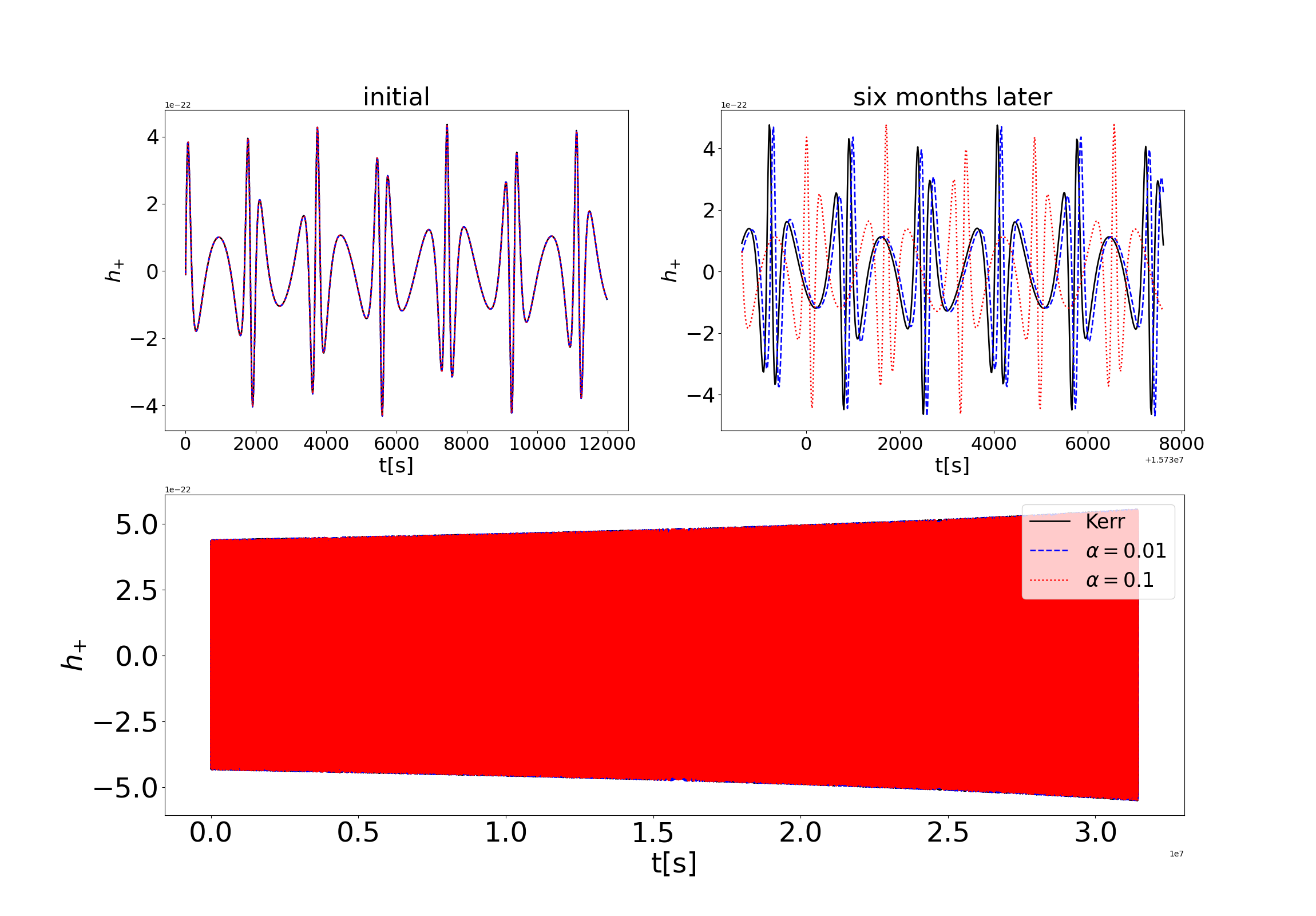
Figure 1: Comparison between the polarizations $h_{+}$ of three EMRI waveforms from the standard Kerr and the quantum-corrected Kerr BHs with derivation parameter $\alpha=(0.01,0.1)$. The BH spin and the initial orbital parameters are chosen to $a=0.9$, $p_{0}=12$ and $e_{0}=0.5$. The left panel of top figures is the initial stage of the time domain waveforms and the right panel of top figures denotes the time domain waveforms after six months. The bottom of figure is the full time domain waveforms of $h_{+}$, where the inspiral time of the CO is set as one year.

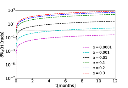
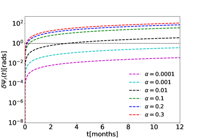
Figure 2: Azimuthal (left) and radial (right) dephasings as functions of the observation time, where the spin of MBH $a=0.9$ and the deviation parameter $\alpha=(0.0001,0.001,0.01,0.1,0.2,0.3)$. The initial orbital semi-latus rectum and and eccentricity are set to $p_{0}=12$ and $e_{0}=0.5$. The horizontal black dashed line in the figures denotes the threshold for phase that can be distinguished by LISA.

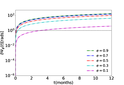
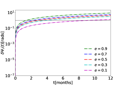
Figure 3: Azimuthal (left) and radial (right) dephasings as functions of the observation time are plotted, where the spin of MBH $a=0.9$ and the deviation parameter $\alpha=0.01$. The initial orbital semi-latus rectum and eccentricity are $p_{0}=12$ and $e_{0}=(0.1,0.3,0.5,0.7,0.9)$. As before, the horizontal black dashed line in the figures denotes the threshold for phase that can be distinguished by LISA.

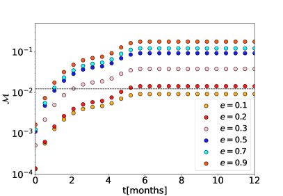
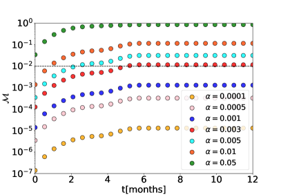
Figure 4: Mismatch between waveforms emitted from EMRI systems with and without the trace anomaly as a function of observation time are plotted, where the length of waveform is set as one year and $a=0.9$. The left panel depicts several cases of eccentricities $e_{0}=(0.1,0.3,0.5,0.7,0.9)$ with $\alpha=0.01$ and $p_{0}=12$, and the right panel shows the examples of different deviation parameters $\alpha=(0.0001,0.0005,0.001,0.003,0.005,0.01,0.05)$ with $e_{0}=0.5$ and $p_{0}=12$. The horizontal black dashed line denotes the minimum value distinguished by LISA.

III.1 Waveform and mismatch

Firstly, we show the comparison of time domain EMRI waveforms in the cases with and without the quantum correction in Fig. 1. Here, we consider the obseravation time for a CO inspiraling into the MBH is one year, and the other parameters are set to $m=30M_{\odot}$, $M=10^{6}M_{\odot}$ $a=0.9$, $\alpha=(0.01,0.1)$, $p_{0}=12$ and $e_{0}=0.5$. As shown in Fig. 1, one can see that the two EMRI waveforms are indistinguishable at the initial stage. However, their distinction becomes prominent after six months of observation. Moreover, we can see that a larger coupling constant $\alpha$ leads to a more significant difference between the two kinds of waveform.

To study the effects from various parameters on the detection capability of LISA for the EMRIs from the QCBHs, we plot the phase difference as a function of observation time by computing the Eq. (30). Following Refs. Datta et al. (2020); Zi and Li (2023a), the threshold value of dephasing is roughly taken as $\delta\Psi^{\rm min}_{r,\phi}=1$ rad, above which the two kinds of signal can be resolved by LISA. The azimuthal and radial dephasing as a function of observation time are plotted in Fig. 2, where the deviation parameter of QCBH with spin $a=0.9$ takes values as $\alpha=(0.0001,0.001,0.01,0.1,0.2,0.3)$. As shown in Fig. 2, the azimuthal and radial dephasing are growing when the deviation parameters $\alpha$ are increasing. To evaluate the impact of orbital eccentricity on the dephasing, we plot several examples of the initial orbital eccentricities $e_{0}=(0.1,0.3,0.5,0.7,0.9)$ in Fig. 3, where the other parameters of QCBH are set as $a=0.9$, $\alpha=0.001$ and $p_{0}=12$. From the Figs. 2 and 3, one can see that the deviation parameter has a more significant influence on the dephasing than the orbital eccentricity. Note that the horizontal black dashed line represents the threshold value of dephasing in the Figs. 2 and 3, so the region above this line means the EMRI waveforms with the quantum correction can be distinguished by LISA.

To quantitatively evaluate the effect of the trace anomaly on the EMRI waveform, the mismatch as a function of observation time is plotted in Fig. 4 with $a=0.9$ and $p_{0}=12$. The left panel shows the mismatch with various values of the eccentricity and a fixed $\alpha=0.01$, while the right panel shows the mismatch with various values of deviation parameter and a fixed eccentricity $e_{0}=0.5$. In both panels the length of waveform is fixed as one year. From the left panel of the figure, one can see that it is possible to distinguish the quantum-corrected waveforms as the orbital eccentrics is bigger. And the distinction between the two kinds of waveform is more evident when the initial orbital eccentricity is bigger. From the right panel, the mismatch between waveforms emitted from the different EMRI systems is sensitive to the deviation parameters, and LISA has the potential to distinguish the quantum-corrected waveform with the deviation parameter as small as $\alpha=0.003$.

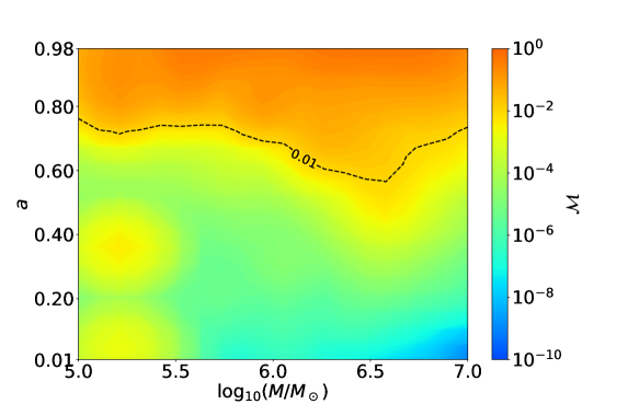
Figure 5: Mismatch as a function of mass and spin of the QCBH with a deviation parameter $\alpha=0.01$ is plotted, where the horizontal black dashed line is the threshold value of mismatch $\mathcal{M}_{\rm min}=0.01$. The other orbital parameters are set as $p_{0}=12$ and $e_{0}=0.5$.

Fig. 5 shows the mismatch as a function of mass and spin of the MBH with the deviation parameter $\alpha=0.01$ and the initial orbital parameters $p_{0}=12$ and $e_{0}=0.5$, considering the one year observation of the EMRI signal. The horizontal black dashed line is the threshold value of the mismatch $\mathcal{M}=0.01$. From this figure, we can find that the mismatch is more sensitive to the spin of the MBH than to its mass. When the spin of the MBH satisfies $a\gtrsim 0.79$, the EMRI waveform with the presence of the trace anomaly can be distinguished by LISA.

III.2 Constraint on the trace anomaly

In this subsection, we perform the parameter estimation for the deviation parameter $\alpha$ using the FIM method. By setting the central values of the $\alpha$ to a given value, we can obtain the constraint on the strength of trace anomaly by LISA. In general, the inspiral is truncated at the last stable orbit of the MBH Stein and Warburton (2020). In this work, by choosing the initial values of the orbital parameters appropriately, we can fix the length of the waveform to one year and keep the inspiral way from the cutoff. The initial orbital parameters are set as $p_{0}=12$ and $e_{0}=0.5$, and the deviation parameter of the MBH is fixed as $\alpha=0.001$. Here we only focus on the effects from the mass and spin of the MBH and let other parameters fixed, since the former ones are more significant.

We plot the parameter estimation uncertainty $\Delta\alpha$ as a function of spin and mass of the MBH in Fig. 6. It is found that the uncertainty of the deviation parameter $\Delta\alpha$ decreases with the spin parameter when the mass of the MBH is fixed. In particular, if the spin of the MBH is small, the uncertainty could exceed the threshold 1, which means $\alpha$ cannot be constrained with EMRI signals in this case. However, the parameter estimation accuracy gets improved quickly with the increase of the spin of the MBH. So the MBH with the largest spin has the best constraint on $\alpha$. We can find that when the spin parameter $a>0.8$ and the mass of the MBH take values around $10^{6}M_{\odot}$, the constraint on the deviation parameter can reach the level of $\sim 10^{-4}$ for one year observation by LISA.

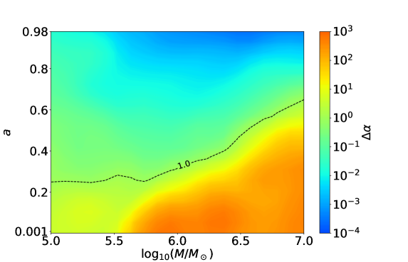
Figure 6: Constraint on the deviation parameter $\Delta\alpha$ as a function of mass and spin of the MBH with $\alpha=0.01$ is plotted, where the black dashed line denotes the threshold value of the measurement error $\Delta\alpha_{\rm max}=1.0$. The initial orbital parameters are set as $p_{0}=12$ and $e_{0}=0.5$.

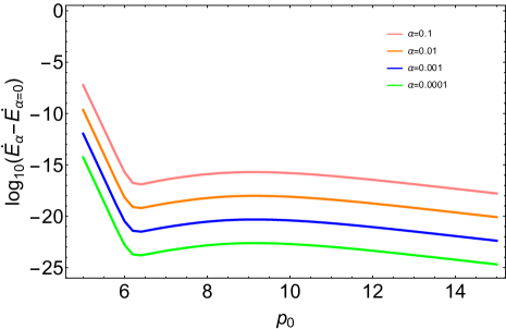
Figure 7: The logarithm of difference values of energy fluxes for the QCBH and Kerr BH as a function of the initial orbital semi-latus rectum for several cases of quantum-corrected parameters $\alpha=(0.0001,0.001,0.01,0.1)$ are plotted. The other orbital parameters are set as $a=0.9$ and $e_{0}=0.5$.

IV Conclusion

In this paper, we computed the gravitational waves emitted from the extreme mass ratio inspirals around rotating BHs in semiclassical gravity sourced by the trace anomaly using the kludge approximate method. We firstly derived the orbital energy, angular momentum and fundamental orbital frequencies for orbits on the equatorial plane. We found that, for the gravitational radiation described by quadrupole formulas, the contribution from the trace anomaly only appears at higher order terms in the the energy flux comparing with the standard Kerr case. Therefore, we evaluated the hybrid orbital evolution equations using the energy flux of Kerr BH, then computed the EMRI waveform with the quadruple formula Barack and Cutler (2004); Barsanti et al. (2022). Moreover, we assessed the differences of phase of the waveforms with and without the trace anomaly by computing the dephasing. Our results indicated that the dephasing is more significant for the larger values of the initial eccentricity $e_{0}$ and the deviation parameter $\alpha$. By computing mismatches of the two kinds of waveform, we found that QCBH with $a\gtrsim 0.79$ can be distinguished from the Kerr BH. According to the parameter estimation of quantum-corrected parameter $\alpha$, the constraints on the parameter $\alpha$ are seriously subjected with the spins of QCBH. In particular, LISA can determine the parameter $\alpha$ within a fractional error of $\sim 10^{-4}$ for the higher spinning QCBH, and EMRI sources with the lower spinning QCBH could not be measurable, especially the more massive QCBH.

It is interesting to perform the study using the complete perturbation theory for the QCBHs, which can provide more accurate EMRI waveforms for the evaluation of the detection ability of the trace anomaly. However, since the horizon of the QCBH is non-spherical, one can expect that the scheme would be much difficult than the Kerr case.

Appendix A Energy flux

In this section we introduce the quadrupole formulas of energy flux derived by Peters and Mathews Peters and Mathews (1963); Peters (1964), where the energy flux can be written as

$$\dot{E}=\frac{1}{5m}\left(\frac{d^{3}I_{ij}}{dt^{3}}\frac{d^{3}I^{ij}}{dt^{3}}-\frac{d^{3}I_{i}^{i}}{dt^{3}}\frac{d^{3}I^{j}_{j}}{dt^{3}},\right)$$ (41)

with the quadrupole moment tensor of mass $I_{ij}$, which can be given by

$$I_{ij}=mx_{i}x_{j},$$ (42)

where $x_{i}$ is the position vector between the smaller object and MBH. Under the weak field approximate condition, we can obtain the formulas of quadrupole moment tensor $Q_{ij}$ and energy flux $\dot{E}$ via the intricate algebraical computation. To illustrate the modification effect of the deviation parameter $\alpha$ on the EMRI energy flux, we plot the logarithmic differences of the energy fluxes from the QCBH and Kerr BH in Fig. 7, the symbols $\dot{E}_{\alpha}$ and $\dot{E}_{\alpha=0}$ denote to the energy flux of QCBH and Kerr BH. From the Fig. 7, one can see that the correction from QCBH on EMRI fluxes can be ignored comparing to the case of the Kerr BH. This is because that the contribution of the deviation parameter $\alpha$ appears at higher order of the weak-field expansion of Eq. (1), that is

$$\mathcal{M}(r,\theta)=M+\frac{2M^{2}\alpha}{r^{3}}+\mathcal{O}\left(\frac{1}{r^{5}}\right).$$ (43)

Therefore, the evolution of orbital parameter in the QCBH spacetime can be approximately addressed with the fluxes of Kerr BH, we adopt the analytic fluxes of energy and angular moment developed by Gair and Glampedakis in Ref. Gair and Glampedakis (2006). The fluxes can be read with our symbol as follows

$$\dot{E} = -\frac{32}{5}\frac{\mu^{2}}{M^{2}}\left(\frac{M}{p}\right)^{5}(1-e^{2})^{3/2}\left[g_{1}(e)-q\left(\frac{M}{p}\right)^{3/2}g_{2}(e)\right.$$

$$\left.-\left(\frac{M}{p}\right)g_{3}(e)+\pi\left(\frac{M}{p}\right)^{3/2}g_{4}(e)\right.$$

$$\left.-\left(\frac{M}{p}\right)^{2}g_{5}(e)+q^{2}\left(\frac{M}{p}\right)^{2}g_{6}(e)-\right.$$

$$\left.\pi\left(\frac{M}{p}\right)^{5/2}g_{7}(e)+q\left(\frac{M}{p}\right)^{5/2}g_{8}(e)\right],\$$

$$\dot{L}_{z} = -\frac{32}{5}\frac{\mu^{2}}{M}\left(\frac{M}{p}\right)^{7/2}(1-e^{2})^{3/2}\left[g_{9}(e)\right.$$ (45)

$$\left.-q\left(\frac{M}{p}\right)^{3/2}g_{10}(e)-\left(\frac{M}{p}\right)g_{11}(e)\right.$$

$$\left.+\pi\left(\frac{M}{p}\right)^{3/2}g_{12}(e)-\left(\frac{M}{p}\right)^{2}g_{13}(e)\right.$$

$$\left.+q^{2}\left(\frac{M}{p}\right)^{2}g_{14}(e)-\pi\left(\frac{M}{p}\right)^{5/2}g_{15}(e)\right.$$

$$\left.+q\left(\frac{M}{p}\right)^{5/2}g_{16}(e)\right],\$$

where the $e$-dependent coefficients are,

$$g_{1}(e) = 1+\frac{73}{24}e^{2}+\frac{37}{96}e^{4},$$

$$g_{2}(e) = \frac{73}{12}+\frac{823}{24}e^{2}+\frac{949}{32}e^{4}+\frac{491}{192}e^{6},$$

$$g_{3}(e) = \frac{1247}{336}+\frac{9181}{672}e^{2},$$

$$g_{4}(e) = 4+\frac{1375}{48}e^{2},$$

$$g_{5}(e) = \frac{44711}{9072}+\frac{172157}{2592}e^{2},$$

$$g_{6}(e) = \frac{33}{16}+\frac{359}{32}e^{2},$$

$$g_{7}(e) = \frac{8191}{672}+\frac{44531}{336}e^{2},$$

$$g_{8}(e) = \frac{3749}{336}-\frac{5143}{168}e^{2},$$

$$g_{9}(e) = 1+\frac{7}{8}e^{2},$$

$$g_{10}(e) = \frac{61}{12}+\frac{119}{8}e^{2}+\frac{183}{32}e^{4},$$

$$g_{11}(e) = \frac{1247}{336}+\frac{425}{336}e^{2},$$

$$g_{12}(e) = 4+\frac{97}{8}e^{2},$$

$$g_{13}(e) = \frac{44711}{9072}+\frac{302893}{6048}e^{2},$$

$$g_{14}(e) = \frac{33}{16}+\frac{95}{16}e^{2},$$

$$g_{15}(e) = \frac{8191}{672}+\frac{48361}{1344}e^{2},$$

$$g_{16}(e) = \frac{417}{56}-\frac{37241}{672}e^{2}.\$$ (46)

Appendix B Stability of the Fisher matrix

In this appendix, following the method in Ref. Piovano et al. (2021); Zi and Li (2023b), we compute the stability of the covariance matrix with the EMRI waveforms. This can be achieved as follows: firstly compute small perturbations of components of Fisher matrices, then see the behavior of covariance matrices. The stability can be characterized quantitatively by the following equation

$$\delta_{\rm stability}\equiv\mathbf{max}_{\rm ij}\left[\frac{((\Gamma+F)^{-1}-\Gamma^{-1})^{ij}}{(\Gamma^{-1})^{ij}}\right]$$ (47)

where $F_{ij}$ is the deviation matrix, the elements is a uniform distribution $U\in[a,b]$. To assess the stability of FIM with the EMRI signal modified by QCBH, we list the results of stability $\delta_{\rm stability}$in the Table 1.

Table 1: The stability $\delta_{\rm stability}$ of FIM with EMRI waveforms from the QCBH with mass $M=10^{6}M_{\odot}$ and $\alpha=0.01$ is computed, including the different spinning caes.

$U$	spin $a$
	$0.1$	$0.3$	$0.5$	$0.7$	$0.9$
$\in[-10^{-6},10^{-6}]$	$3.47\times 10^{-1}~{}~{}$	$2.11\times 10^{-1}$	$6.82\times 10^{-2}$	$3.65\times 10^{-2}$	$2.72\times 10^{-4}$
$\in[-10^{-9},10^{-9}]$	$9.64\times 10^{-2}~{}~{}$	$3.82\times 10^{-3}$	$7.16\times 10^{-4}$	$3.07\times 10^{-4}$	$1.35\times 10^{-4}$

References

- Fernandes (2023) P. G. S. Fernandes, Phys. Rev. D 108, L061502 (2023), arXiv:2305.10382 [gr-qc] .
- Abbott et al. (2016) B. P. Abbott et al. (LIGO Scientific, Virgo), Phys. Rev. Lett. 116, 061102 (2016), arXiv:1602.03837 [gr-qc] .
- Abbott et al. (2019) B. P. Abbott et al. (LIGO Scientific, Virgo), Phys. Rev. X 9, 031040 (2019), arXiv:1811.12907 [astro-ph.HE] .
- Abbott et al. (2021a) R. Abbott et al. (LIGO Scientific, Virgo), Phys. Rev. X 11, 021053 (2021a), arXiv:2010.14527 [gr-qc] .
- Abbott et al. (2021b) R. Abbott et al. (LIGO Scientific, VIRGO, KAGRA), (2021b), arXiv:2111.03606 [gr-qc] .
- Abbott et al. (2021c) R. Abbott et al. (LIGO Scientific, VIRGO, KAGRA), (2021c), arXiv:2112.06861 [gr-qc] .
- Abbott et al. (2022a) R. Abbott et al. (LIGO Scientific, Virgo, KAGRA), Phys. Rev. D 105, 102001 (2022a), arXiv:2111.15507 [astro-ph.HE] .
- Abbott et al. (2023) R. Abbott et al. (LIGO Scientific, Virgo, KAGRA), Astrophys. J. 949, 76 (2023), arXiv:2111.03604 [astro-ph.CO] .
- Abbott et al. (2022b) R. Abbott et al. (LIGO Scientific, KAGRA, Virgo), Phys. Rev. D 105, 063030 (2022b), arXiv:2105.13085 [astro-ph.CO] .
- Nagano et al. (2019) K. Nagano, T. Fujita, Y. Michimura, and I. Obata, Phys. Rev. Lett. 123, 111301 (2019), arXiv:1903.02017 [hep-ph] .
- Abbott et al. (2020) R. Abbott et al. (LIGO Scientific, Virgo), Astrophys. J. Lett. 900, L13 (2020), arXiv:2009.01190 [astro-ph.HE] .
- Patricelli (2021) B. Patricelli (LIGO Scientific, Virgo), in 19th Lomonosov Conference on Elementary Particle Physics (2021).
- Cardoso and Pani (2019) V. Cardoso and P. Pani, Living Rev. Rel. 22, 4 (2019), arXiv:1904.05363 [gr-qc] .
- Cardoso and Pani (2017) V. Cardoso and P. Pani, Nature Astron. 1, 586 (2017), arXiv:1709.01525 [gr-qc] .
- Cardoso et al. (2016) V. Cardoso, E. Franzin, and P. Pani, Phys. Rev. Lett. 116, 171101 (2016), [Erratum: Phys.Rev.Lett. 117, 089902 (2016)], arXiv:1602.07309 [gr-qc] .
- Maggio et al. (2019) E. Maggio, A. Testa, S. Bhagwat, and P. Pani, Phys. Rev. D 100, 064056 (2019), arXiv:1907.03091 [gr-qc] .
- Arun et al. (2022) K. G. Arun et al. (LISA), Living Rev. Rel. 25, 4 (2022), arXiv:2205.01597 [gr-qc] .
- Robinson (1975) D. C. Robinson, Phys. Rev. Lett. 34, 905 (1975).
- Barack and Cutler (2007) L. Barack and C. Cutler, Phys. Rev. D 75, 042003 (2007), arXiv:gr-qc/0612029 .
- Cardoso and Gualtieri (2016) V. Cardoso and L. Gualtieri, Class. Quant. Grav. 33, 174001 (2016), arXiv:1607.03133 [gr-qc] .
- Zi et al. (2021) T.-G. Zi, J.-D. Zhang, H.-M. Fan, X.-T. Zhang, Y.-M. Hu, C. Shi, and J. Mei, Phys. Rev. D 104, 064008 (2021), arXiv:2104.06047 [gr-qc] .
- Newman et al. (1965) E. T. Newman, R. Couch, K. Chinnapared, A. Exton, A. Prakash, and R. Torrence, J. Math. Phys. 6, 918 (1965).
- Chrusciel et al. (2012) P. T. Chrusciel, J. Lopes Costa, and M. Heusler, Living Rev. Rel. 15, 7 (2012), arXiv:1205.6112 [gr-qc] .
- Berti et al. (2015) E. Berti et al., Class. Quant. Grav. 32, 243001 (2015), arXiv:1501.07274 [gr-qc] .
- Barack et al. (2019) L. Barack et al., Class. Quant. Grav. 36, 143001 (2019), arXiv:1806.05195 [gr-qc] .
- Liebling and Palenzuela (2023) S. L. Liebling and C. Palenzuela, Living Rev. Rel. 26, 1 (2023), arXiv:1202.5809 [gr-qc] .
- Raposo and Pani (2020) G. Raposo and P. Pani, Phys. Rev. D 102, 044045 (2020), arXiv:2002.02555 [gr-qc] .
- Sanchis-Gual et al. (2021) N. Sanchis-Gual, F. Di Giovanni, C. Herdeiro, E. Radu, and J. A. Font, Phys. Rev. Lett. 126, 241105 (2021), arXiv:2103.12136 [gr-qc] .
- Hawking (1975) S. W. Hawking, Commun. Math. Phys. 43, 199 (1975), [Erratum: Commun.Math.Phys. 46, 206 (1976)].
- Capper and Duff (1974) D. M. Capper and M. J. Duff, Nuovo Cim. A 23, 173 (1974).
- Duff (1994) M. J. Duff, Class. Quant. Grav. 11, 1387 (1994), arXiv:hep-th/9308075 .
- Anderson et al. (2007) P. R. Anderson, E. Mottola, and R. Vaulin, Phys. Rev. D 76, 124028 (2007), arXiv:0707.3751 [gr-qc] .
- Mottola and Vaulin (2006) E. Mottola and R. Vaulin, Phys. Rev. D 74, 064004 (2006), arXiv:gr-qc/0604051 .
- Mottola (2017) E. Mottola, JHEP 07, 043 (2017), [Erratum: JHEP 09, 107 (2017)], arXiv:1606.09220 [gr-qc] .
- Yang et al. (2022) S.-J. Yang, Y.-P. Zhang, S.-W. Wei, and Y.-X. Liu, JHEP 04, 066 (2022), arXiv:2201.03381 [gr-qc] .
- Jiang and Zhang (2023) J. Jiang and M. Zhang, Eur. Phys. J. C 83, 687 (2023), arXiv:2305.12345 [gr-qc] .
- Zhang et al. (2023) Z. Zhang, Y. Hou, M. Guo, and B. Chen, (2023), arXiv:2305.14924 [gr-qc] .
- Gurses and Tekin (2023) M. Gurses and B. Tekin, (2023), arXiv:2310.00312 [gr-qc] .
- Amaro-Seoane et al. (2017) P. Amaro-Seoane et al. (LISA), (2017), arXiv:1702.00786 [astro-ph.IM] .
- Luo et al. (2016) J. Luo et al. (TianQin), Class. Quant. Grav. 33, 035010 (2016), arXiv:1512.02076 [astro-ph.IM] .
- Ruan et al. (2020) W.-H. Ruan, Z.-K. Guo, R.-G. Cai, and Y.-Z. Zhang, Int. J. Mod. Phys. A 35, 2050075 (2020), arXiv:1807.09495 [gr-qc] .
- Berry et al. (2019) C. P. L. Berry, S. A. Hughes, C. F. Sopuerta, A. J. K. Chua, A. Heffernan, K. Holley-Bockelmann, D. P. Mihaylov, M. C. Miller, and A. Sesana, (2019), arXiv:1903.03686 [astro-ph.HE] .
- Berti et al. (2019) E. Berti et al., (2019), arXiv:1903.02781 [astro-ph.HE] .
- Gair et al. (2004) J. R. Gair, L. Barack, T. Creighton, C. Cutler, S. L. Larson, E. S. Phinney, and M. Vallisneri, Class. Quant. Grav. 21, S1595 (2004), arXiv:gr-qc/0405137 .
- Amaro-Seoane et al. (2007) P. Amaro-Seoane, J. R. Gair, M. Freitag, M. Coleman Miller, I. Mandel, C. J. Cutler, and S. Babak, Class. Quant. Grav. 24, R113 (2007), arXiv:astro-ph/0703495 .
- Babak et al. (2017) S. Babak, J. Gair, A. Sesana, E. Barausse, C. F. Sopuerta, C. P. L. Berry, E. Berti, P. Amaro-Seoane, A. Petiteau, and A. Klein, Phys. Rev. D 95, 103012 (2017), arXiv:1703.09722 [gr-qc] .
- Fan et al. (2020) H.-M. Fan, Y.-M. Hu, E. Barausse, A. Sesana, J.-d. Zhang, X. Zhang, T.-G. Zi, and J. Mei, Phys. Rev. D 102, 063016 (2020), arXiv:2005.08212 [astro-ph.HE] .
- Kocsis et al. (2011) B. Kocsis, N. Yunes, and A. Loeb, Phys. Rev. D 84, 024032 (2011), arXiv:1104.2322 [astro-ph.GA] .
- Barausse et al. (2014) E. Barausse, V. Cardoso, and P. Pani, Phys. Rev. D 89, 104059 (2014), arXiv:1404.7149 [gr-qc] .
- Cardoso et al. (2022) V. Cardoso, K. Destounis, F. Duque, R. Panosso Macedo, and A. Maselli, Phys. Rev. Lett. 129, 241103 (2022), arXiv:2210.01133 [gr-qc] .
- Dai et al. (2023) N. Dai, Y. Gong, Y. Zhao, and T. Jiang, (2023), arXiv:2301.05088 [gr-qc] .
- Figueiredo et al. (2023) E. Figueiredo, A. Maselli, and V. Cardoso, Phys. Rev. D 107, 104033 (2023), arXiv:2303.08183 [gr-qc] .
- Zi and Li (2023a) T. Zi and P.-C. Li, Phys. Rev. D 108, 084001 (2023a), arXiv:2306.02683 [gr-qc] .
- Rahman et al. (2023a) M. Rahman, S. Kumar, and A. Bhattacharyya, (2023a), arXiv:2306.14971 [gr-qc] .
- Rahman et al. (2023b) M. Rahman, S. Kumar, and A. Bhattacharyya, JCAP 01, 046 (2023b), arXiv:2212.01404 [gr-qc] .
- Kumar et al. (2023) S. Kumar, A. Chowdhuri, and A. Bhattacharyya, (2023), arXiv:2311.05983 [gr-qc] .
- Sago and Tanaka (2021) N. Sago and T. Tanaka, Phys. Rev. D 104, 064009 (2021), arXiv:2106.07123 [gr-qc] .
- Maggio et al. (2021) E. Maggio, M. van de Meent, and P. Pani, Phys. Rev. D 104, 104026 (2021), arXiv:2106.07195 [gr-qc] .
- Zhang et al. (2021) Y.-P. Zhang, Y.-B. Zeng, Y.-Q. Wang, S.-W. Wei, P. A. Seoane, and Y.-X. Liu, (2021), arXiv:2108.13170 [gr-qc] .
- Datta and Bose (2019) S. Datta and S. Bose, Phys. Rev. D 99, 084001 (2019), arXiv:1902.01723 [gr-qc] .
- Datta et al. (2020) S. Datta, R. Brito, S. Bose, P. Pani, and S. A. Hughes, Phys. Rev. D 101, 044004 (2020), arXiv:1910.07841 [gr-qc] .
- Pani and Maselli (2019) P. Pani and A. Maselli, Int. J. Mod. Phys. D 28, 1944001 (2019), arXiv:1905.03947 [gr-qc] .
- De Luca et al. (2023) V. De Luca, A. Maselli, and P. Pani, Phys. Rev. D 107, 044058 (2023), arXiv:2212.03343 [gr-qc] .
- Zi and Li (2023b) T. Zi and P.-C. Li, Phys. Rev. D 108, 024018 (2023b), arXiv:2303.16610 [gr-qc] .
- Agullo et al. (2021) I. Agullo, V. Cardoso, A. D. Rio, M. Maggiore, and J. Pullin, Phys. Rev. Lett. 126, 041302 (2021), arXiv:2007.13761 [gr-qc] .
- Datta and Phukon (2021) S. Datta and K. S. Phukon, Phys. Rev. D 104, 124062 (2021), arXiv:2105.11140 [gr-qc] .
- Eichhorn and Held (2021a) A. Eichhorn and A. Held, Eur. Phys. J. C 81, 933 (2021a), arXiv:2103.07473 [gr-qc] .
- Eichhorn and Held (2021b) A. Eichhorn and A. Held, JCAP 05, 073 (2021b), arXiv:2103.13163 [gr-qc] .
- Delaporte et al. (2022) H. Delaporte, A. Eichhorn, and A. Held, Class. Quant. Grav. 39, 134002 (2022), arXiv:2203.00105 [gr-qc] .
- Gair and Glampedakis (2006) J. R. Gair and K. Glampedakis, Phys. Rev. D 73, 064037 (2006), arXiv:gr-qc/0510129 .
- Glampedakis and Kennefick (2002) K. Glampedakis and D. Kennefick, Phys. Rev. D 66, 044002 (2002), arXiv:gr-qc/0203086 .
- Barack and Cutler (2004) L. Barack and C. Cutler, Phys. Rev. D 69, 082005 (2004), arXiv:gr-qc/0310125 .
- Canizares et al. (2012) P. Canizares, J. R. Gair, and C. F. Sopuerta, Phys. Rev. D 86, 044010 (2012), arXiv:1205.1253 [gr-qc] .
- Apostolatos et al. (1994) T. A. Apostolatos, C. Cutler, G. J. Sussman, and K. S. Thorne, Phys. Rev. D 49, 6274 (1994).
- Cutler (1998) C. Cutler, Phys. Rev. D 57, 7089 (1998), arXiv:gr-qc/9703068 .
- Flanagan and Hughes (1998) E. E. Flanagan and S. A. Hughes, Phys. Rev. D 57, 4566 (1998), arXiv:gr-qc/9710129 .
- Lindblom et al. (2008) L. Lindblom, B. J. Owen, and D. A. Brown, Phys. Rev. D 78, 124020 (2008), arXiv:0809.3844 [gr-qc] .
- Vallisneri (2008) M. Vallisneri, Phys. Rev. D 77, 042001 (2008), arXiv:gr-qc/0703086 .
- Zi et al. (2023) T. Zi, Z. Zhou, H.-T. Wang, P.-C. Li, J.-d. Zhang, and B. Chen, Phys. Rev. D 107, 023005 (2023), arXiv:2205.00425 [gr-qc] .
- Stein and Warburton (2020) L. C. Stein and N. Warburton, Phys. Rev. D 101, 064007 (2020), arXiv:1912.07609 [gr-qc] .
- Barsanti et al. (2022) S. Barsanti, N. Franchini, L. Gualtieri, A. Maselli, and T. P. Sotiriou, Phys. Rev. D 106, 044029 (2022), arXiv:2203.05003 [gr-qc] .
- Peters and Mathews (1963) P. C. Peters and J. Mathews, Phys. Rev. 131, 435 (1963).
- Peters (1964) P. C. Peters, Phys. Rev. 136, B1224 (1964).
- Piovano et al. (2021) G. A. Piovano, R. Brito, A. Maselli, and P. Pani, Phys. Rev. D 104, 124019 (2021), arXiv:2105.07083 [gr-qc] .