Williams, Gartner, and Harper

Predictive and Prescriptive Analytics for Modeling Frail and Elderly Patient Services

Predictive and Prescriptive Analytics for Multi-Site Modeling of Frail and Elderly Patient Services

Elizabeth M. Williams, Daniel Gartner and Paul R. Harper School of Mathematics, Cardiff University, williamsem20@cardiff.ac.uk, gartnerd@cardiff.ac.uk, harper@cardiff.ac.uk

1. Problem definition: Recent research has highlighted the potential of linking predictive and prescriptive analytics. However, it remains widely unexplored how both paradigms could benefit from one another to address today’s major challenges in healthcare. One of these is smarter planning of resource capacities for frail and elderly inpatient wards, addressing the societal challenge of an aging population. Frail and elderly patients typically suffer from multimorbidity and require more care while receiving medical treatment. The aim of this research is to assess how various predictive and prescriptive analytical methods, both individually and in tandem, contribute to addressing the operational challenges within an area of healthcare that is growing in demand. 2. Methodology/results: Clinical and demographic patient attributes are gathered from more than 165,000 patient records and used to explain and predict length of stay. To that extent, we employ Classification and Regression Trees (CART) analysis to establish this relationship. On the prescriptive side, deterministic and two-stage stochastic programs are developed to determine how to optimally plan for beds and ward staff with the objective to minimize cost. Furthermore, the two analytical methodologies are linked by generating demand for the prescriptive models using the CART groupings. The results show the linked methodologies provided different but similar results compared to using averages and in doing so, captured a more realistic real-world variation in the patient length of stay. 3. Managerial implications: Our research reveals that healthcare managers should consider using predictive and prescriptive models to make more informed decisions. By combining predictive and prescriptive analytics, healthcare managers can move away from relying on averages and incorporate the unique characteristics of their patients to create more robust planning decisions, mitigating risks caused by variations in demand. Ultimately, this can lead to improved health outcomes and more efficient allocation of resources.

Health Care Management; Math Programming; Stochastic Methods Submitted:

1 Introduction

Aging populations put pressure on both the economy and healthcare resources world-wide with medical care expenditures on the rise (United Nations 2019). Aging is one of the most common and well-known risk factors for most chronic diseases (Macnee et al. 2014). According to United Nations (2019), an elderly person can be defined as 65 years old and over, whilst a frail person is classified as one who is at high risk of falling into dependency as a result of a negative event, such as an injury, fall or disability (Xue 2011). Care for frail and elderly patients has more challenges and barriers in providing care due to a lack of resources or specialized models for care delivery (Heydari et al. 2019). Frail and elderly patients often suffer from multi-morbidity and can take longer to recover in a hospital with more staffing hours and resources required. These patients not only share resources with other patient types but are unique in terms of having their own service specialty within hospitals, known as care of the elderly (COTE). A common problem faced is the inability to discharge these patients within a timely manner causing excessive bed blocking within hospitals (Zychlinski et al. 2021). There is often difficulty in grouping these patients together for length of stay (LOS) prediction, as there are many different factors which cause longer lengths of stay.

To address these challenges, healthcare analytics has proven beneficial in dealing with a wide array of planning challenges in healthcare. The use of analytical techniques has the potential to save up to 25% in annual costs in healthcare (Dash et al. 2019). The recent COVID-19 pandemic has demonstrated the crucial need for analytics to be used and continually developed within the healthcare setting to provide highly beneficial results. The main challenges faced by healthcare managers are the hundreds of beds and staff to manage, which creates an excessive number of options for decisions (Best et al. 2015). Demand and capacity are further complicated because no two patients are exactly alike. Because bed capacity planning typically relies on averages, it fails to take into consideration the stochastic nature of the healthcare industry (Harper and Shahani 2002). This research aims to contribute to the literature by incorporating natural variability through the use of classification and regression trees (CART).

To the best of our knowledge, this is the first study to examine the value of linking predictive and prescriptive analytics for the capacity planning of frail and elderly healthcare resources. We approach the problem in two steps. Firstly, we learn classification and regression trees (CART) from a large dataset and identify groupings of patients aged 65 and over with similar attributes that affect the LOS in hospital. Secondly, we develop a deterministic and stochastic mixed-integer program for the planning of bed and staffing resources. Thirdly, we apply the CART-based groupings to the developed deterministic and two-stage stochastic model analyzing capacity demands in a multi-hospital network setting. Finally, we analyze the value of the stochastic solution (VSS), to determine the benefits of implementing the stochastic model over the traditional deterministic model. The results of this research will provide valuable insights for healthcare managers, highlighting the importance of considering multiple analytics methods to make informed decisions. By understanding the value of predictive and prescriptive analytics, healthcare managers can avoid traps by planning resources based on averages. This, in turn, can lead to better health outcomes and more efficient use of resources.

The remainder of the paper is structured as follows. Section 2 provides an overview of current literature in terms of CART analysis with a particular focus on frail and elderly patients. Moreover, deterministic and stochastic optimization models for hospital bed planning are compared and contrasted with our work. In Section 3, we firstly outline the mathematical methodology for CART, deterministic and two-stage stochastic models. Then, we introduce an illustrative example to demonstrate the models’ functionality. In Section 4, we apply our models to real-world data from a network of hospitals, introducing variation into the model by utilizing CART predictions for demands. Then, we provide comparisons between the deterministic and two-stage stochastic models by calculating the value of the stochastic solution (VSS). Our paper concludes with Section 5 including a discussion and directions for future research.

2 Related Work

This section aims to provide insight into existing operational research (OR) literature specifically focusing on hierarchical CART methodologies along with deterministic and stochastic modeling techniques. The first subsection will focus on CART analysis applied to frail and elderly patients and the second subsection will focus on deterministic and stochastic modeling techniques applied to healthcare settings.

A wide variety of literature reviews have been published within the healthcare OR field. On a broader scale, previous healthcare reviews have discussed how data analytics can be applied (Mišić and Perakis 2020). The authors detailed the need for deployment of data analytics at different levels, including policy, hospital, and patient-specific. Typically, literature reviews are more focused on specific methods (Morid et al. 2017), (Ahmadi-Javid et al. 2017) or patient types (Williams et al. 2021). Morid et al. (2017) explored the application of supervised machine learning techniques for predicting healthcare costs, whilst Ahmadi-Javid et al. (2017) conducted a comprehensive review into optimization methods specifically applied to outpatient appointment scheduling. Williams et al. (2021) presented a literature review highlighting the use of Operational Research and Management Science (OR/MS) methodologies in addressing the challenges associated with the care of frail and elderly patients. These reviews demonstrate a wide variety of research taking place within the healthcare domain. Our research aims to overlap between these reviews, by applying OR methodologies to elderly and frail patient care.

2.1 CART Analysis Applied to Frail and Elderly

CART is a machine learning method for constructing prediction models from data. The algorithm constructs a decision tree which is structured hierarchically. The decision tree asks a series of questions that decide groups into which the data is sorted, in the form of binary recursive partitioning, where each node is split into two groups. CART analysis has often been applied to healthcare for predictive analytics, covering a wide range of medical settings. Within frail and elderly care, the literature can be grouped into two subgroups. The first grouping focuses on illnesses typically suffered by these patients, with the second grouping having a more generic medical setting however using elderly and frail as the patient groups of interest.

2.1.1 Use of CART within Hospitals

The works of Byeon (2015), Ius et al. (2020) and Watanabe et al. (2018), demonstrated the use of CART models within hospitals. These papers either focus on including age as a variable in their CART model or have subset their patients so only a certain age range are included. Byeon (2015) developed a prediction tool using CART of endocrine disorders in the elderly. Although age was not included as a variable in the model, only patients aged over 60 were included in the analysis. Byeon was able to determine categories of patients who had a higher prevalence of clinical conditions including depression and obesity. Similarly, Ius et al. (2020) applied random forests, an extension of CART, to identify whether age was a factor in the treatment of glioblastoma in the elderly. The authors identified similar characteristics of patients to provide a score performance on the terminal nodes. This risk score was then applied through survival analysis of Kaplan-Meier curves to determine overall survival against time. By utilizing age as a continuous variable, the authors were able to conclude that age did influence overall survival, although did not have the largest influence. Watanabe et al. (2018) applied CART to determine different risk factors of rotator cuff tears between elderly and young patients. By using age as a continuous variable, the authors identified that age had the greatest influence on tears. The next category of splitting is then different depending on the age group of the patient. The work conducted by these three authors demonstrates that CART has successfully been applied to a range of illnesses suffered by the elderly.

2.1.2 Use of CART across Hospitals and Community Care

Expanding to hospital and community wide care, Kuo et al. (2019), Lam et al. (2019) and Passmore et al. (1993) demonstrate how CART can also be applied to wider healthcare settings. Kuo et al. (2019) used CART models to develop a system for identifying social frailty in the elderly. A range of 15 variables was incorporated, including: age, BMI, income and marital status. Random forests and C5.0 classification models were found to have the highest prediction accuracy of 0.970. The tool built allows the probability of social frailty to be determined based on the values for the 15 variables inputted. Lam et al. (2019) used CART to identify whether frailty would be an indicator of recurrent fallers over the age of 65 in the community. The authors calculated three different frailty indexes and grouped the patients by both age and gender. The results showed that certain frailty indexes did have a high predictive ability of recurrent falls, although were only significant in female patients. Passmore et al. (1993) used certain characteristics of elderly patients to determine unplanned admission into hospital. A sickness impact profile (SIP) score provided the health status of each of the patients and was identified to be the most influential factor in predicting hospitalization. The authors also identified that the number of medications prescribed to the patients had an influencing factor and provided further scope for preventative steps to avoid admissions.

These six papers demonstrate the success of applying CART to frail and elderly patients when considering both care setting and the medical condition suffered. This research aims to build upon the previous literature in this field by considering how different hospital locations determine a patient’s LOS. Additionally, a further variety of data types which may have an impact on patient stays within hospitals, such as radiological data, will be incorporated.

2.2 Multi-site Deterministic and Stochastic Healthcare Modeling

Deterministic modeling is popular within healthcare settings due to its ease of application, however, traditionally many healthcare services are stochastic in nature (Mandelbaum et al. 2018).

2.2.1 Deterministic Models

Hare et al. (2009) and Segall (1992) analyzed deterministic modeling within healthcare settings. Hare et al. (2009) developed a deterministic multi-state Markov model to plan for services within home and community care. The authors decided upon five age groups, three of which encompass the elderly. Additionally, the authors incorporated the changing age and health demographics of the patient groups to determine how service use will change over time. Segall (1992) extended a disaggregated resource allocation model to include a demand constraint, to determine spacial allocation of resources. Applying to 16 acute care hospitals and then to the entire state of Massachusetts, the author was able to determine occupancy rates and demands for hospitals, specialties and predict the average LOS.

2.2.2 Stochastic Models

The works of Abdelaziz and Masmoudi (2012), Guo et al. (2021), Levis and Papageorgiou (2004) and Thompson et al. (2009) applied stochastic modeling techniques to healthcare settings. Abdelaziz and Masmoudi (2012) determined the number of beds to be assigned to hospital departments given random demand in order to minimize costs of beds and the number of physicians and nurses working. By using a multi-objective stochastic program, the authors grouped specialties by primary, secondary and tertiary levels where demand varies and is required to be satisfied. The authors were able to consider a network of 157 public hospitals to determine the optimal number of beds and staffing. Guo et al. (2021) applied logic-based benders decomposition and binary decision diagram based approaches to optimize surgery scheduling within operating rooms. The authors introduce two and three-stage decomposition approaches to incorporate the stochastic nature of surgical care, e.g., surgeries being canceled or the time each procedure takes. Guo et al. were able to successfully generate more robust schedules which in turn reduced the rate of cancellation and improve the rate or operating room utilization. Levis and Papageorgiou (2004) applied stochastic capacity planning to the pharmaceutical industry. Pharmaceutical products are manufactured in two stages and then transported either to hospitals or clinical testing sites upon successful approval. The authors provided five examples of where multi-site, multi-period capacity planning problems are solved with uncertain clinical trial outcomes and customer demand. Thompson et al. (2009) used Markov decision processes to plan short-term allocation of patients during demand surges. The authors aimed to determine the best patient assignments and reduce the cost from transferring patients.

2.2.3 Deterministic and Stochastic Models

Mestre et al. (2015) used location allocation models with both deterministic and stochastic approaches for the planning and designing of a network of hospitals. The authors aim to inform decision-makers on how to improve access to different healthcare services and specialties whilst minimizing costs. By generating two models, the authors determined the impact of the allocation within both the first and second stages. They were able to successfully conclude that by including both location and allocation within the first stage, the model was more flexible in terms of hospital network planning, allowing the second stage to incorporate unsatisfied demand and extra capacities.

These five papers display the variety of both deterministic and stochastic modeling applications within healthcare. These models will be built upon to determine where specific specialties should be located based on demand locations when focusing on a subgroup of patients. The benefits will be determined by using either deterministic or stochastic modeling will be shown.

2.3 Main Contributions and Literature Summary

In conclusion, our search of the literature has revealed gaps in linking predictive and prescriptive analytics to optimize resource allocation under uncertainty in healthcare. Current literature relies heavily on deterministic optimization models for healthcare planning, which fail to capture inherent variability. We bridge this gap by integrating data-driven predictive modelling with stochastic optimization. Specifically, we use CART to generate demand inputs for a two-stage stochastic program, creating a robust optimization model. This combination of predictive and prescriptive analytics differentiates our work from existing literature. Additionally, our focus on an integrated network of hospitals providing elderly care contrasts with single-site models that dominate previous studies. Furthermore, our joint optimization of staffing and bed capacity is unique compared to other papers that optimize these decisions separately. Finally, the explicit incorporation of specialty and acuity mix for frail elderly patients differs from previous studies. In summary, the multi-site, integrated resource planning, predictive forecasting, stochastic optimization and an explicit elderly patient focus, represent key contributions to the healthcare operations literature.

In terms of the deterministic and stochastic models, our approach follows the approach of Maggioni and Wallace (2013). Our work extends this two-fold: first, by providing a healthcare example and second, by incorporating CART models into the demand function to create real-world variation into the formulation. We extend this work by providing a healthcare example and incorporating CART models into the modeling formulation.

Second, we research an area of healthcare which has been under-researched, despite the increased demand and medical needs of these patients (Williams et al. 2021).

Finally, with respect to methodology, we provide a different perspective on how this could be modeled. Previous bed and staffing capacity models have focused on neural networks (Kutafina et al. 2019), queuing theoretical approaches (Ghayoomia et al. 2022, de Véricourt and Jennings 2011, Yankovic and Green 2011), simulation (Amelia et al. 2021, Lu et al. 2021). Our methodology builds on traditionally used deterministic methods in healthcare by demonstrating the benefits of using stochastic models by calculating the VSS.

3 Methods

This section will discuss the approaches used within this paper, providing the notation used to allow the reader to apply the theories to their own work. There is a large amount of variation in terms of hospital LOS. We have carefully chosen these methods to allow easy incorporation of this variation. CART was chosen over other predictive methodologies because it offers a visual representation. This makes it possible for healthcare practitioners to comprehend and trust the model’s output, with the potential for collaboration to create clinical and statistically meaningful groupings. Due to the complexity of our problem, a mixed integer programming approach is used, allowing the LOS variation to be integrated into the bed and staffing planning simultaneously.

3.1 Classification and Regression Trees

Classification and regression trees (CART) is a data mining technique in which variables predict an outcome. Classification trees are used for categorical dependent variables and the algorithm predicts the class, whereas regression trees are used for continuous dependent variables and the algorithm predicts the value. The parameters that make up the final groups are visually represented by a decision tree. The decision tree asks a series of questions that decide the groups into which the data is sorted. CART models are a form of binary recursive partitioning, where each node is split into two groups. A visual representation of a decision tree is shown within Figure 1.

Figure 1: Example of a decision tree with one root node, three decision nodes and five terminal nodes.

Within both classification and regression trees, categorical variables are present within the data. Because of the nature of the algorithm, the variables have to undergo preprocessing to change these to numerical data. Since there is no ordinal relationship in the categorical data, one-hot encoding must be used to convert to integer encoding. Each distinct integer value is represented by a brand-new binary variable, which replaces the categorical variable. The newly one-hot encoded variables can then be run with the numerical variables into the CART algorithm.

3.1.1 General Formulation

To determine the best splits on the algorithm, the CART methods utilize two different measures. Regression trees utilize the mean squared error (MSE) and classification trees utilize the Gini Index. The MSE informs the user as to how much their prediction deviates from the original target, and is calculated as follows:

$$\text{MSE}=\frac{1}{n}\sum^{n}_{i=1}(Y_{i}-\hat{Y}_{i})^{2}$$ (1)

where $n$ is the number of observations, $Y_{i}$ is the actual value and $\hat{Y}_{i}$ is the predicted value.

The Gini Index determines the optimal splitting choice for classification trees. The Gini Index yields a number between 0 and 1, with a smaller value indicating greater sample homogeneity. The Gini Index is calculated as follows:

$$\text{Gini Index}=1-\sum_{i=1}^{n}p_{i}^{2}$$ (2)

where $i$ is the number of classes and $p_{i}$ is the probability of an object that is being classified to a particular class.

3.1.2 Feature Parameters

The CART algorithm has a number of parameters that can be altered to improve the model. The splitting process continues recursively until a stopping criterion is met, such as reaching a maximum tree depth, a minimum number of data points per leaf node, or a minimum decrease in impurity. At each internal node, a feature parameter is selected to split the data based on its ability to discriminate between the target variable’s classes or to reduce the prediction error.

3.1.3 Evaluation Metrics

To ascertain success and how well the model predicts LOS, a series of evaluation measures can be applied to each of the different CART models.

Regression trees are evaluated using the $R^{2}$ value. The $R^{2}$ is the coefficient of determination and calculates how good a model’s fit is compared to a given dataset. The $R^{2}$ value is calculated as follows:

$$R^{2}=1-\frac{\sum^{n}_{i=1}(Y_{i}-\hat{Y}_{i})}{\sum^{n}_{i=1}(Y_{i}-\bar{Y}_{i})}$$ (3)

where $Y_{i}$ represents the true $y$ value, $\hat{Y}_{i}$ is the value of the predicted $y$ value, $\bar{Y}_{i}$ represents the mean of all values and $n$ is the total number of observations. The higher the $R^{2}$ value, the more accurate the model is.

3.2 Deterministic and Two-Stage Stochastic Programming

Within this section the deterministic and stochastic mathematical programs will be discussed, providing the notation used to allow the reader to apply the theories to their own work. The aim of the model is to determine the number of beds and nursing staff required for each specialty within each hospital. The motivation for choosing these resources stems from their pivotal roles in shaping healthcare service delivery. Beds directly influence patient capacity, while nursing staff are instrumental in ensuring high-quality patient care and operational efficiency. Importantly, the allocation of these resources is inherently intertwined, as the number of beds required directly affects the staffing needs, and vice versa.

This research will follow the framework as used by Mestre et al. (2015) and Maggioni and Wallace (2010).

3.2.1 General Formulation

Let us define the two-stage stochastic problem, where a decision-maker takes the decision $x$ of solution space X to minimize expected costs:

$$\min_{x\in X}E_{\boldsymbol{\xi}}z(x,\boldsymbol{\xi})=\min_{x\in X}\left\{f_{1}(x)+E_{\boldsymbol{\xi}}\left[h_{2}(x,\boldsymbol{\xi})\right]\right\}$$ (4)

where $x$ are the first-stage decision variables restricted to the set $X\subset\mathbb{R}^{n}$ and $f_{1}(x)$ is the value of the first stage problem. $E_{\boldsymbol{\xi}}$ indicates the expectation with respect to a random vector denoted $\boldsymbol{\xi}$ defined on the probability space $(\Omega,\mathscr{A},p)$, with $\Omega\in\mathbb{R}^{n}$ and probability distribution p on the $\sigma$-algebra $\mathscr{A}$.

The function $h_{2}(x,\xi)$ is the value function of the second stage of the stochastic problem, defined as follows:

$$h_{2}(x,\xi)=\min_{y\in Y(x,\xi)}f_{2}(y:x,\xi)$$ (5)

where $y$ is the second-stage solution which is restricted to the set $Y\in\mathbb{R}^{n}$.

Equation (5) reflects the costs associated with the information being revealed through the realization of $\xi$ from the random vector $\boldsymbol{\xi}$. The term $\left[h_{2}(x,\boldsymbol{\xi})\right]$, is known as the recourse function.

The solution obtained is defined as the ‘here and now solution’ (RP) and is the optimal value of the objective function:

$$RP=E_{\boldsymbol{\xi}}z(x^{*},\boldsymbol{\xi})$$ (6)

Equation (4) can be considered where the decision-maker replaces the random variables with their expected values and in turn, solves a deterministic model. This is also known as the expected value problem.

$$EV=\min_{x\in X}z(x,\bar{\xi})$$ (7)

where $\bar{\xi}=E(\boldsymbol{\xi})$, which is the expected value of the random vector $\xi$ and $z$ is the objective value.

3.2.2 Sets

Table 1 displays the sets used within the deterministic and two-stage stochastic models. The sets are used to define the parameters and variables within the model. The sets are defined as follows:

Set	Range	Definition
$\mathcal{B}$	b = 1,…, B	Set of nursing bands
$\mathcal{S}$	s = 1,…, S	Set of specialties
$\mathcal{H}$	h = 1,…, H	Set of hospitals
$\mathcal{R}$	r = 1,…, R	Set of regions
$\mathcal{K}$	k = 1,…, K	Set of scenarios

Table 1: The sets used within the two-stage stochastic model where (B,S,H,R,K) represent the maximum number of nursing bands, specialties, hospitals, regions and scenarios, respectively.

Each of the specialties must appear in at least one of the hospitals ($\mathcal{S}\subseteq\mathcal{H}$). Similarly, each of the hospitals must appear in one of the regions ($\mathcal{H}\subseteq\mathcal{R}$). Therefore $|\mathcal{H}|\leq|\mathcal{R}|$.

3.2.3 Parameters

Table 2 displays the parameters used within the deterministic and two-stage stochastic models:

Parameter	Definition
c${}^{\textnormal{bed, 1st}}_{s,h}$	Cost of the first stage beds for specialty $s\in\mathcal{S}$, in hospital $h\in\mathcal{H}$
c${}^{\textnormal{bed, 2nd}}_{s,h}$	Cost of the second stage bed per day for specialty $s\in\mathcal{S}$, in hospital $h\in\mathcal{H}$
c${}^{\textnormal{staff, 1st}}_{b}$	Cost of the first stage staff of band $b\in\mathcal{B}$
c${}^{\textnormal{staff, 2nd}}_{b}$	Cost of the second stage staff of band $b\in\mathcal{B}$
pk	Probability of scenario $k\in\mathcal{K}$
Ds,r,k	Demand for each specialty $s\in\mathcal{S}$, arriving from region $r\in\mathcal{R}$, for scenario $k\in\mathcal{K}$
Rs,b	Ratio of nursing staff of band $b\in\mathcal{B}$ to patient for each specialty $s\in\mathcal{S}$
$K_{s,h}$	Number of beds available to open in each specialty $s\in\mathcal{S}$, in hospital $h\in\mathcal{H}$
UB${}^{\textnormal{max, bed, 1st}}_{h}$	Upper bound of the number of beds that are able to be deployed in hospital $h\in\mathcal{H}$ in the 1st stage
UB${}^{\textnormal{max, bed, 2nd}}_{h}$	Upper bound of the number of beds that are able to be deployed in hospital $h\in\mathcal{H}$ in the $2^{nd}$ stage
UB${}^{\textnormal{max, staff, 1st}}_{b}$	Upper bound of the number of staff that can be deployed in the $1^{st}$ stage
UB${}^{\textnormal{max, staff, 2nd}}_{b}$	Upper bound of the number of staff that can be deployed in the $2^{nd}$ stage

Table 2: The parameters used within the two-stage stochastic model where (b,s,h,r,k) represent the maximum number of nursing bands, specialties, hospitals, regions and scenarios, respectively.

3.2.4 Decision Variables

The decision variables introduced in Table 3 determine the number of beds and nursing staff required for each specialty within each hospital.

Decision Variable	Definition
$x^{\textnormal{bed}}_{s,h}\in\mathbb{N}$	Number of beds planned in the $1^{st}$ stage for specialty $s\in\mathcal{S}$, in hospital $h\in\mathcal{H}$
$x^{\textnormal{staff}}_{s,b,h}\in\mathbb{N}$	Number of staff planned in the $1^{st}$ stage for specialty $s\in\mathcal{S}$, of band $b\in\mathcal{B}$, in hospital $h\in\mathcal{H}$
$u^{\textnormal{bed}}_{s,r,h,k}\in\mathbb{N}$	Number of beds needed in the $2^{nd}$ stage for specialty $s\in\mathcal{S}$, for patients arriving from
	region $r\in\mathcal{R}$ in hospital $h\in\mathcal{H}$, for scenario $k\in\mathcal{K}$
$u^{\textnormal{staff}}_{s,b,h,k}\in\mathbb{N}$	Number of staff needed in the $2^{nd}$ stage for specialty $s\in\mathcal{S}$, of band $b\in\mathcal{B}$, in hospital $h\in\mathcal{H}$,
	for scenario $k\in\mathcal{K}$

Table 3: The decision variables used within the two-stage stochastic model where ($b,s,h,r,k$) represent the value number of nursing bands, specialties, hospitals, regions and scenarios, respectively.

3.2.5 Model

Using the introduced sets, parameters and decision variables, the deterministic model can be defined as follows:

$$\text{min}\sum_{h\in\mathcal{H}}\sum_{s\in\mathcal{S}}(c^{\textnormal{bed}}_{s,h}x^{\textnormal{bed}}_{s,h}+\sum_{b\in\mathcal{B}}c^{\textnormal{staff}}_{b}x^{\textnormal{staff}}_{s,b,h})$$ (8)

subject to:

$$\sum_{h\in\mathcal{H}}x^{\textnormal{bed}}_{s,h} \geq D_{s,r} \forall s\in\mathcal{S},r\in\mathcal{R}$$ (9)

$$\sum\limits_{b^{\prime}\in\mathcal{B}:b^{\prime}\geq b}x^{\textnormal{staff}}_{s,b^{\prime},h} \geq R_{s,b}\cdot x^{\textnormal{bed}}_{s,h} \forall s\in\mathcal{S},b\in\mathcal{B},h\in\mathcal{H}$$ (10)

$${x_{s,h}^{\textnormal{bed}}} \leq K_{s,h} \forall s\in\mathcal{S},h\in\mathcal{H}$$ (11)

$$0\leq\sum_{s\in\mathcal{S}}{x_{s,h}^{\textnormal{bed}}} \leq{UB_{h}^{\textnormal{max, bed}}} \forall h\in\mathcal{H}$$ (12)

$$0\leq\sum_{s\in\mathcal{S}}\sum_{h\in\mathcal{H}}{x_{s,b,h}^{\textnormal{staff}}} \leq UB^{\textnormal{max, staff}}_{b} \forall b\in\mathcal{B}$$ (13)

Objective function (8) minimizes the cost of deploying beds and staff in each specialty and hospital. Constraints (9) ensure the number of beds deployed satisfies the demand. Constraints (10) make sure the number of staff deployed to each specialty within each hospital meets the minimum requirements. Constraints (11) ensure the number of beds deployed cannot exceed the maximum available specialty beds within each hospital. Constraints (12)–(13) denote the decision variables and their domains

Similarly, the two-stage stochastic model can be defined as follows:

$$\text{min}\sum_{h\in\mathcal{H}}\sum_{s\in\mathcal{S}}(c^{\textnormal{bed, 1st}}_{s,h}x^{\textnormal{bed}}_{s,h}+\sum_{b\in\mathcal{B}}c^{\textnormal{staff, 1st}}_{b}x^{\textnormal{staff}}_{s,b,h})\\ +\sum_{k\in\mathcal{K}}\sum_{h\in\mathcal{H}}\sum_{s\in\mathcal{S}}p_{k}(c^{\textnormal{bed, 2nd}}_{s,h}u^{\textnormal{bed}}_{s,h,k}+\sum_{b\in\mathcal{B}}c^{\textnormal{staff, 2nd}}_{b}u^{\textnormal{staff}}_{s,b,k,h})$$ (14)

subject to:

$$\sum_{h\in\mathcal{H}}({x_{s,h}^{\textnormal{bed}}}+{u_{s,h,k}^{\textnormal{bed}}}) \geq D_{s,r,k} \forall s\in\mathcal{S},r\in\mathcal{R},k\in\mathcal{K}$$ (15)

$$\sum\limits_{b^{\prime}\in\mathcal{B}:b^{\prime}\geq b}{x_{s,b^{\prime},h}^{\textnormal{staff}}} \geq R_{s,b}\cdot{x_{s,h}^{\textnormal{bed}}} \forall s\in\mathcal{S},b\in\mathcal{B},h\in\mathcal{H}$$ (16)

$$\sum\limits_{b^{\prime}\in\mathcal{B}:b^{\prime}\geq b}u_{s,b^{\prime},k,h}^{\textnormal{staff}} \geq R_{s,b}\cdot{u_{s,h,k}^{\textnormal{bed}}} \forall s\in\mathcal{S},b\in\mathcal{B},h\in\mathcal{H},k\in\mathcal{K}$$ (17)

$${x_{s,h}^{\textnormal{bed}}} \leq K_{s,h} \forall s\in\mathcal{S},h\in\mathcal{H}$$ (18)

$${u_{s,h,k}^{\textnormal{bed}}} \leq K_{s,h} \forall s\in\mathcal{S},h\in\mathcal{H},k\in\mathcal{K}$$ (19)

$$0\leq\sum_{s\in\mathcal{S}}{x_{s,h}^{\textnormal{bed}}} \leq{UB_{h}^{\textnormal{max, bed, 1st}}} \forall h\in\mathcal{H}$$ (20)

$$0\leq\sum_{s\in\mathcal{S}}\sum_{h\in\mathcal{H}}{x_{s,b,h}^{\textnormal{staff}}} \leq{UB_{b}^{\textnormal{max, staff, 1st}}} \forall b\in\mathcal{B}$$ (21)

$$0\leq\sum_{s\in\mathcal{S}}{u_{s,h,k}^{\textnormal{bed}}} \leq{UB_{h}^{\textnormal{max, bed, 2nd}}} \forall h\in\mathcal{H},k\in\mathcal{K}$$ (22)

$$0\leq\sum_{s\in\mathcal{S}}\sum_{h\in\mathcal{H}}{u_{s,b,k,h}^{\textnormal{staff}}} \leq{UB_{b}^{\textnormal{max, staff, 2nd}}} \forall b\in\mathcal{B},k\in\mathcal{K}$$ (23)

The first sum in the objective function (14) is the cost of deploying both beds and staff to specialties within each hospital. The second sum represents the additional beds and staff within the same hospital or a different hospital in the same region. The first constraint, (15), assures the demand for each specialty and region is met by the number of hospital beds deployed. The demand is dependent on the scenario parameter. Constraints (16) ensures the number of staff deployed meets the minimum requirements for staff on each specialty ward in the first stage, whilst Constraints (17) ensures this requirement is met in the second stage. Constraints (18) and (19) ensures the beds deployed do not exceed the maximum number of beds available for each specialty within each hospital. Constraints (20)–(23) denote the decision variables and their domains.

3.2.6 Evaluation of Measures

Within prescriptive analytics, it is widely recognized that the EV solution can behave poorly in the stochastic domain. Traditional evaluation tests can be carried out in order to determine how each of the EV, RP and EEV performs and determine their robustness. Maggioni and Wallace (2010) discussed four tests to determine the success of stochastic models. For this research, the first method of determining the value of the stochastic solution (VSS) will be used.

If we let $\bar{x}(\bar{\xi})$ be the optimal solution to Equation (7), we can take values and fix these as the first stage, and then allow the second stage of the stochastic model to be performed.

$$EEV=E_{\boldsymbol{\xi}}(z(\bar{x}(\bar{\xi}),\boldsymbol{\xi}))$$ (24)

To determine the VSS, the difference between the EEV and RP can be calculated, measuring the expected increase in value from solving the stochastic solution to the simple deterministic one:

$$VSS=EEV-RP$$ (25)

The VSS measures expected loss when using the deterministic solution. If we have hard constraints, the expected cost of the deterministic solution is often $\infty$. Whereas if we use soft constraints, we can make the expected cost arbitrarily bad by setting penalties high using the deterministic solution. If the VSS is large, this could mean the wrong choice of variables has been chosen or the wrong values have been entered.

3.2.7 Illustrative Example

To demonstrate the applicability of our proposed model, we have included a small worked example with fictional numerical values to illustrate the optimization process and key outputs. A small number of scenarios have been included within the second stage to provide a simple illustration of the stochastic programming approach, while retaining computational traceability. A dataset of 15 patients can be used to demonstrate how the model performs in the application of elderly and frail patient care (Table 4).

Patient Number Age Hospital LOS Specialty Admission Method Admission Source Frailty Source Patient 1 95 1 5 COTE Emergency Own Home 3 Patient 2 82 1 3 COTE Emergency Own Home 2 Patient 3 89 1 4 T&O Emergency Own Home 2 Patient 4 87 1 4 T&O Elective Own Home 2 Patient 5 85 2 3 COTE Elective Transferred 1 Patient 6 76 2 1 COTE Elective Transferred 1 Patient 7 71 2 1 T&O Emergency Transferred 1 Patient 8 96 1 5 T&O Emergency Own Home 3 Patient 9 70 2 1 COTE Emergency Transferred 1 Patient 10 67 2 1 T&O Elective Own Home 1 Patient 11 89 1 4 COTE Elective Transferred 3 Patient 12 70 2 1 COTE Elective Own Home 2 Patient 13 75 2 4 T&O Elective Transferred 3 Patient 14 72 2 2 COTE Elective Transferred 3 Patient 15 87 1 5 COTE Emergency Own Home 2

Table 4: Worked Example Patient Data - 15 Patients

Within the dataset there are two hospitals within the same region, each serving the same two specialties: care of the elderly (COTE) and trauma and orthopedics (T&O). We assume there are two nursing staff band levels required on the wards, with differing staff/bed ratios depending on the specialty. Table 5 shows the parameters and their corresponding values for the deterministic and stochastic models.

Parameters	Values	Parameters	Values
1st Stage Bed Costs ($c^{\textnormal{bed,1st}}_{s,h}$)	$\begin{bmatrix}20&30\\ 30&40\end{bmatrix}$	2nd Stage Bed Costs ($c^{\textnormal{bed,2nd}}_{s,h}$)	$\begin{bmatrix}22&33\\ 33&44\end{bmatrix}$
Ratio ($R_{s,b}$)	$\begin{bmatrix}0.29&0.14\\ 0.14&0.29\end{bmatrix}$	Maximum Specialty Capacity ($K_{s,h}$)	$\begin{bmatrix}20&25\\ 20&25\\ \end{bmatrix}$
1st Stage Staff Costs ($c^{\textnormal{staff, 1st}}_{b}$)	[$\pounds 50,\pounds 60$]	2nd Stage Staff Costs ($c^{\textnormal{staff, 2nd}}_{b}$)	[$\pounds 55,\pounds 66$]
Upper 1st bed limit ($UB^{\textnormal{max,bed,1st}}_{h}$)	[20,25]	Upper 2nd bed limit ($UB^{\textnormal{max,bed,2nd}}_{h,k}$)	$\begin{bmatrix}20&20&20\\ 25&25&25\end{bmatrix}$
Upper 1st staff limit ($UB^{\textnormal{max,staff,1st}}_{b}$)	[15,25]	Upper 2nd staff limit ($UB^{\textnormal{max,staff,2nd}}_{b.k}$)	$\begin{bmatrix}15&15\\ 25&25\end{bmatrix}$
Probability of Scenarios ($p_{k}$)	[0.4,0.3,0.3]

Table 5: The parameter values that were used within the deterministic and two-stage stochastic model specifically for the illustrative example.

The demand from Table 4 can be calculated as follows to determine the average daily bed demand:

$${\text{Average daily bed demand}_{s,h}=\text{Average LOS}_{s,h}\times\text{Average daily number of admissions}_{s,h}}$$ (26)

$${D_{s,r}=\text{Average daily bed demand}_{s,r}=\sum_{h\in\mathcal{R}}\text{Average daily bed demand}_{s,h}}$$ (27)

This produces a value of 16.67 and 19.01 for the D_0,0 and D_1,0 parameters, respectively. For the two-stage stochastic model, a number of scenarios are required. For this example and to demonstrate the model’s functionality, we introduce three scenarios which average to the same deterministic demand: Average demand with a probability of 40%, demand increasing by 20% with a probability of 30%, demand decreasing by 20% with a probability of 30%.

Therefore the demand matrix $D_{s,r,k}$ can be represented as: $\begin{bmatrix}[16.66,19.99,13.33]\\ [19.01,22.80,15.20]\end{bmatrix}$, where the first index refers to the row and the second index refers to the column. In this instance we only have one region, therefore only one column matrix is shown. The third index refers to the column inside the sub-matrix. Table 6 displays the optimal decision variables and objective function values for the worked example.

	s=0, h=0	s=0, h=1	s=1, h=0	s=1, h=1	Objective Value ($\pounds$)
EV	[(0), (0,0)]	[(17), (5, 3)]	[(20), (3, 6)]	[(0), (0, 0)]	2,050.00
RP	[(20), (6, 3)]	[(1), (1, 1)]	[(24), (4, 8)]	[(0), (0, 0)]	2,185.20
EEV	[(4), (2, 1)]	[(17), (5, 3)]	[(24), (4, 8)]	[(0), (0, 0)]	2,240.80

Table 6: Deterministic and Two-Stage Stochastic Results for the Worked Example - Results are Recorded [(beds), (staff)]

The results reveal that the deterministic model deploys fewer beds and nursing staff than the stochastic model, leading to an EV solution that costs approximately two-thirds of the RP. The EEV value is calculated by fixing the first-stage decision variables in the two-stage stochastic model with the optimal values from the deterministic model. This then calculates the values for the second-stage variables and the objective function value. The VSS is then calculated to be the difference between the EEV and RP, resulting in a value of $\pounds$55.60, a saving of 2.54%, if the stochastic solution were to be implemented. The results also show that the deterministic model is not robust, as the EEV is greater than the RP. This is due to the deterministic model not being able to account for the uncertainty in the demand.

4 Case Study of a Network of Hospitals in the U.K.

Three years’ worth of data covering the period April 2017 to March 2020 was provided by a large NHS trust in the U.K. Data prior to the COVID-19 pandemic was used to ensure the data was not skewed. A total of 165,188 records of patients aged 65 and over were included in the study. This spanned a total of 29 different specialties and 11 different hospital sites.

4.1 Results of CART Analysis

This section discusses the development and results of the CART models. This section will be split into two subsections, the first for regression trees (Section 4.1.1) and the second for classification trees (Section 4.1.2). The results of the CART analysis will be used to inform the deterministic and stochastic models.

4.1.1 Regression Trees

Regression trees were developed to predict the LOS of patients. Admission method, admission source, age (as a continuous and grouped measure), day, diagnosis, frailty (as a continuous and grouped), hospital, number of scans and specialty were the nine variables used within the regression trees.

Age and frailty were included as continuous and grouped variables to determine which would be more appropriate for the regression trees. The models were trained on 80% of the data with a 20% test set being used to validate the models.

The ‘Scikit-learn’ package within Python was used to generate the regression trees utilizing the ‘DecisionTreeRegressor’ function. The default parameters were utilized within the model with the exception of the ‘max_leaf_nodes’ and the ‘min_samples_leaf’ parameters. The default parameters have been successfully employed in other studies (Hancock and Khoshgoftaar 2022, Heyburn et al. 2018, Kilincer et al. 2023). These ‘max_leaf_nodes’ and the ‘min_samples_leaf’ parameters underwent parameter optimization through a step wise approach. This was to ensure underfitting and overfitting were avoided (Bramer 2007). Additionally, we wanted to set the upper limit of the ‘max_leaf_nodes’ to a manageable amount of groupings. The parameters used have been provided within Table 2 in the Supplementary Material and were selected based on the default values and parameter optimization to determine the largest $R^{2}$ score.

The largest $R^{2}$ score was achieved by grouping age into five-year intervals and using frailty as a continuous measure. This value was calculated to be 34.23%. Whilst this is a low $R^{2}$ score, it is expected due to the large variation in LOS within the data (417 days). This result shows the model correctly assigns patients to the correct node 34.23% of the time.

4.1.2 Classification Trees

Classification trees were also developed to predict patients who were discharged on the same day or admitted overnight. In addition to the nine variables used within the regression trees, month was also included as a predictor, since it was found to be a significant variable within logistic regression analysis. Similar to the regression trees, the model was performed with both age and frailty as a continuous and grouped measure to determine which would be more appropriate. The models were trained on 80% of the data with a 20% test set being used to validate the models. The ‘DecisionTreeClassifier’ function was used to develop the classification trees using the ‘Scikit-learn’ package within Python. The parameters used for the ‘DecisionTreeClassifier’ function are shown in Table 2 in the Supplementary Material. The accuracy score was calculated to be 89.89% when age was grouped and frailty was used as a continuous measure whilst using one minimum sample per leaf and 30 maximum leaf nodes. The groupings determined by the end nodes of the CART models can be used to determine the demand for each specialty within each hospital.

4.2 Results of the Deterministic vs. Stochastic Multi-site Model

This subsection will utilize the average demand for each specialty and each region from the three years’ worth of data, and feed this into the deterministic and two-stage stochastic model.

The 11 healthcare locations can be grouped into six different regions, offering 29 specialties across all hospitals. In practice, there are 90 combinations of where specialties can be located, with not all hospitals offering every specialty. Within the NHS, there are different levels of nursing staff, ranging from band two to band eight. The higher the band, the more senior the staff member. Two levels of nursing bands will be used to develop the models (bands five and six). In order to gather costing figures, open source data from Public Health Scotland (2021) was used. The costing data and parameter values are shown in Table 1 in the Supplementary Material for reference.

In order to meet the demand and satisfy the constraints, the deterministic model utilized the first-stage variables only. The results yielded a yearly cost of $\pounds$904,280.80. In total, 1,027 beds across different hospitals were deployed with Figure 2 displaying the precise locations of these beds. In order to satisfy demand a total of 414 NHS nurses across a 24-hour period were required.

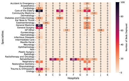
Figure 2: Heatmap of bed locations for each specialty within each hospital for the deterministic model.

The two-stage stochastic model was considered with three different years of data in each scenario, with weightings based on the number of admissions per year. This approach aims to ascertain, drawing insights from past performance, the most effective strategies for future planning and decision-making.

• Year one (2017-2018) with a probability of 32.25%

• Year two (2018-2019) with a probability of 33.95%

• Year three (2019-2020) with a probability of 32.80%

The average of all scenarios is equal to the deterministic daily demands.

The results of the stochastic model yielded a yearly cost of $\pounds$923,827.91. In total, 941 beds are deployed within the first stage, with a maximum of 337 in the second stage. Similarly, 86 additional nursing staff are deployed across both stages of the model compared to the deterministic counterpart. The location of the 1,278 beds can be seen within Figure 3.

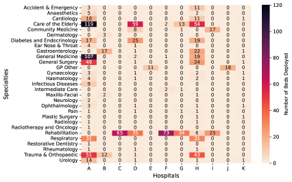
Figure 3: Heatmap of bed locations for each specialty within each hospital for the two-stage stochastic model.

To determine the robustness of the deterministic model, the VSS was calculated, by fixing the results from the deterministic model as the first stage within the two-stage stochastic model. The VSS was calculated to be $\pounds$35,438.97 over a year period, a saving of $\approx$ 3.84% (Table 7). This shows that the deterministic model is not robust, as the EEV is greater than the RP. This is due to the deterministic model not being able to account for the uncertainty in the demand.

	Total Beds		Total Staff		Objective Value ($\pounds$)
	$x^{\textnormal{bed}}$	$u^{\textnormal{bed}}$	$x^{\textnormal{staff}}$	$u^{\textnormal{staff}}$
EV	1,026	-	414	-	904,280.80
RP	941	337	346	154	923,827.91
EEV	1,026	186	414	104	959,266.86

Table 7: The EV, RP and EEV values for the $x^{\textnormal{bed}}$, $x^{\textnormal{staff}}$, $u^{\textnormal{bed}}$ and $u^{\textnormal{staff}}$ decision variables and the objective function value.

4.3 Results of Linking the Two Paradigms

To investigate linking these two paradigms, two methods have been explored and applied to both the classification tree and regression tree results. The first method calculated the number of patients of each specialty and the overall average LOS for each end node. The second method used each end node and the specific LOS for each specialty and hospital within the node. These were then summed together to form the D_s,r parameter.

4.3.1 Regression Tree and Average LOS

The first method utilized the regression tree generated previously, which generated 30 patient groupings determined by the 30 leaf nodes. The average LOS determined by each node was used to calculate the demand for each node. Using Equation (28), the average demand was calculated as follows:

$$D_{s,r}=\sum\limits_{h\in r}D_{s,h}=\frac{\text{Number of Patients}_{s,h}\times\text{Node Average LOS}}{\text{Total Number of Days in Dataset}}$$ (28)

Table 8 presents the results from the demands generated using the average LOS. The same three scenarios, as listed previously, were applied to the demand figures for the two-stage stochastic model. The VSS can be calculated to be 3.52% with a saving of $\pounds$32,435.33. In comparison to Table 7, there was a difference in the deterministic solution of approximately 0.04%, with the regression tree deploying fewer numbers of beds and nurses. Surprisingly, COTE specialty produced the largest individual specialty cost in the stochastic model compared to the deterministic case. This significant savings for COTE was achieved due to better capturing the variation in demand through the stochastic approach. The model outputs can be used to provide tailored recommendations, with particular focus on wards and specialties exhibiting higher demand variability.

	Total Beds		Total Staff		Objective Value ($\pounds$)
	$x^{\textnormal{bed}}$	$u^{\textnormal{bed}}$	$x^{\textnormal{staff}}$	$u^{\textnormal{staff}}$
EV	1,014	-	410	-	903,905.00
RP	925	333	344	158	922,295.07
EEV	1,014	172	410	102	954,730.40

Table 8: The EV, RP and EEV values for the $x^{\textnormal{bed}}$, $u^{\textnormal{bed}}$, $x^{\textnormal{staff}}$, $u^{\textnormal{staff}}$ decision variables and objective function using the regression tree and the average LOS across all three years.

4.3.2 Regression Tree and Specific LOS

Instead of utilizing the average LOS for each of the 30 end nodes, the specific LOS for each hospital and specialty inside that node was calculated. Each of the demands’ generation processes is shown in Equation (29).

$$D_{s,r}=\sum\limits_{h\in r}D_{s,h}=\frac{\text{Number of Patients}_{s,h}\times{\text{Specific LOS}_{s,h}}}{\text{Total Number of Days in Dataset}}$$ (29)

The findings for the deterministic and two-stage stochastic models are shown in Table 9, with the EEV also being calculated to determine the VSS.

	Total Beds		Total Staff		Objective Value ($\pounds$)
	$x^{\textnormal{bed}}$	$u^{\textnormal{bed}}$	$x^{\textnormal{staff}}$	$u^{\textnormal{staff}}$
EV	1,016	-	410	-	889,227.00
RP	922	366	346	158	913,565.80
EEV	1,008	191	410	102	947,256.62

Table 9: The EV, RP and EEV values for the $x^{\textnormal{bed}}$, $u^{\textnormal{bed}}$, $x^{\textnormal{staff}}$, $u^{\textnormal{staff}}$ decision variables and objective function using the regression tree and the specific LOS across all three years.

The specific LOS model had the same deterministic objective function value function however a lower two-stage stochastic objective value as compared to the regression tree with average LOS findings. This shows that if the exact LOS was used, rather than node averages, additional cost savings would be produced. The VSS produced a saving of $\pounds$33,690.82 per day (3.69%), highlighting using the stochastic model would be beneficial.

4.3.3 Classification Tree and Average LOS

The third method utilized the classification tree, which also yielded 30 patient groupings, with patients falling into one of two categories. Equation (28) was used to create demands and to calculate the D_s,r variable.

The results using these demands are shown in Table 10. By deploying 1,009 beds and 388 nurses, an EV value of $\pounds$886,167.60 was produced. Similar to prior findings, fewer beds were used than the averages produced in Section 4.2. A significant reduction in the total objective function resulted from the deployment of beds to different hospital locations.

	Total Beds		Total Staff		Objective Value ($\pounds$)
	$x^{\textnormal{bed}}$	$u^{\textnormal{bed}}$	$x^{\textnormal{staff}}$	$u^{\textnormal{staff}}$
EV	1,009	-	388	-	886,167.60
RP	915	351	332	160	906,864.40
EEV	1,009	178	388	102	939,304.60

Table 10: The EV, RP and EEV values for the $x^{\textnormal{bed}}$, $u^{\textnormal{bed}}$, $x^{\textnormal{staff}}$, $u^{\textnormal{staff}}$ decision variables and objective function using the classification tree and the average LOS across all three years.

The VSS was calculated to be 3.58%, demonstrating that savings may still be achieved using this strategy even when classification trees are used to generate the demand.

4.3.4 Classification Tree and Specific LOS

Instead of utilizing the average LOS for each of the 30 end nodes, the LOS was calculated for each hospital and specialty inside that node. The generation of each demand is shown in Equation (29).

Table 11 presents the results for the deterministic and two-stage stochastic model, with the EEV also being calculated to determine the VSS.

	Total Beds		Total Staff		Objective Value ($\pounds$)
	$x^{\textnormal{bed}}$	$u^{\textnormal{bed}}$	$x^{\textnormal{staff}}$	$u^{\textnormal{staff}}$
EV	1,002	-	422	-	840,245.40
RP	911	343	348	162	862,154.89
EEV	1,002	185	422	98	894,197.68

Table 11: The EV, RP and EEV values for the $x^{\textnormal{bed}}$, $u^{\textnormal{bed}}$, $x^{\textnormal{staff}}$, $u^{\textnormal{staff}}$ decision variables and objective function using the classification tree and the specific LOS across all three years.

Comparing to the regression tree with average LOS results, the deterministic and two-stage stochastic objective values were higher in the specific LOS model. This suggested that using node averages might not produce sufficient capacity for beds and staff. The VSS produced a saving of $\pounds$32,042.79 per day (3.72%).

These results demonstrate the ability to use the CART models to generate the demand for the deterministic and stochastic models. The VSS values produced from the regression tree and classification tree were similar, with the regression tree producing slightly higher savings. This enables the ability to be able to perform scenario analysis, and specifically targetting leaf nodes from the CART models to determine the impact on the system and requirements for beds. As age demographics are expected to change over time, the patient age groupings can be altered to determine the impact on the system. By using each individual year’s data as a scenario, planning for the future can be more informed and adaptable, allowing for better decision-making and resource allocation in anticipation of various potential outcomes.

4.4 Managerial Insights and Generalizability of the Results

The results discussed can provide guidance and recommendations for enhancing healthcare bed and staffing allocations. One key takeaway from the models is the clear demonstration of the drawbacks of planning solely based on averages. This eye-opening insight has underscored the importance of adopting more sophisticated and dynamic approaches to resource planning, steering the health board away from potential pitfalls in their decision-making process. Perhaps the most impactful aspect of this project lies in its utilization of predictive modeling, specifically within the healthcare domain. For a healthcare provider who is accustomed to simpler average models, this research has showcased the true potential of mathematical modeling, revealing its power in unraveling complexities, optimizing operations, and delivering data-driven insights into healthcare planning.

Generalizing results is a critical aspect of research that helps to ensure that the findings of a study are relevant and applicable beyond the specific context in which they were obtained. This makes it possible to guarantee that the study will be beneficial and instructive for other academics, professionals, and policymakers who could be working in other locations or with various populations. The deterministic and two-stage stochastic equations are able to be applied to any healthcare scenario. Whilst this research particularly focused on frail and elderly patients, due to the changing population demographics within the area, the equations can be applied to other age groupings. The benefit of using CART models is that researchers and clinicians can apply the theory to their own patient types and identify distinctive homogeneous clusters of patient features. As time passes and the demographic of patients changes, these models can be rerun to determine new patient clusters. The user can choose the number of hospitals in each region and the range of specialties they may provide because of the equations’ structure, which allows the models to be adjusted to fit any size region. Whilst these models were run with three levels of nursing bands, these can be increased or decreased to suit the user. Additionally, if decision-makers wanted to determine the needs for other hospital resources such as ventilators, these could be easily added to the model. The models are adaptable and reliable to suit a variety of healthcare situations.

5 Summary and Conclusions

By linking predictive and prescriptive analytics, decision-makers can obtain a comprehensive view of their data and use it to make better decisions. For example, if predictive analytics indicates there is a high likelihood of a certain event occurring in the future, prescriptive analytics can recommend specific actions that can be taken to mitigate the risk or take advantage of the opportunity. Furthermore, this integration can also allow decision-makers to continuously improve their decision-making processes over time. By tracking the effectiveness of their decisions and making adjustments based on new data and insights, they can optimize their operations and achieve better outcomes.

There are potential avenues for future work following this research. One aspect could take hospital utilization into consideration and consider a more holistic approach, for example, if emergency department utilization is high then patients are more likely to be discharged from hospital. Additionally, a time constraint to plan on specific time periods rather than on a longer-term time scale. This would create a more dynamic model which would take seasonal demand changes into consideration. Reinforcement learning of the two paradigms could be used to reward the CART predictive models for demand classifications that improve outcomes from the stochastic programming prescriptive models. Finally, an important area for future research is conducting a comprehensive sensitivity analysis to identify which parameters and modeling assumptions have the biggest potential impact on cost savings and resource optimization. This will allow us to prioritize refinements that can further improve the predictive and prescriptive models.

This research has discussed how predictive and prescriptive analytics could be used in combination for efficiently planning hospital specialty beds and staffing requirements for a network of hospitals in the U.K. By comparing the regression tree and classification results to the averages, it allowed differences to be determined and validation of the linked methods to take place. The results showed regression trees produced closer results to the averages. The validation of these regression trees paves the way for more complex scenario analysis to be able to take place.

The authors would like to acknowledge the generous support and contributions from NHS staff in the Aneurin Bevan University Health Board as well as the financial contribution from the Knowledge Economy Skills Scholarship (KESS2). KESS2 is a pan-Wales higher level skills initiative led by Bangor University on behalf of the Higher Education sector in Wales. It is part funded by the Welsh Government‘s European Social Fund (ESF) convergence programme for East Wales.

Appendix

Attribute	Data type	Distinct attribute values or bins	Documentation
Admission Date	Ordinal	1,096 (e.g. 01/04/2017)	at admission
Admission Method	Nominal	17 (e.g. Elective waiting list)	at admission
Admission Source	Nominal	26 (e.g. Usual place of residence)	at admission
Admission Time	Continuous	1440 ({hh:mm})	at admission
Borough	Nominal	174 (e.g. Newport LHB, Monmouthshire LHB)	at admission
Date of birth	Ordinal	12037 (e.g. 01/01/1940)	at admission
Diagnosis	Nominal	2758 (e.g. Fracture of neck of femur, Congestive heart failure)	at admission
Discharge Date	Ordinal	1154 (e.g. 01/04/2017)	at discharge
Discharge Destination	Nominal	26 (e.g. Death, Own home, Patient transfer within same health board/trust)	at discharge
Discharge Time	Continuous	1306 ({hh:mm:ss})	at discharge
Hospital	Nominal	14 (e.g. Chepstow Community Hospital)	at admission
NHS Number	Nominal	66251 (e.g. 4900000000)	at admission
Postcode	Nominal	13819 (e.g. CF72 8XR)	at admission
Registered GP	Nominal	1313 (e.g. G9041668)	at admission
Registered GP Practice	Nominal	618 (e.g. W93012)	at admission
Scan Attendance Date	Ordinal	1097 (e.g. (01/04/2017)	during admission
Scan Attendance Time	Continuous	11417 ({hh:mm:ss})	during admission
Scan Exam	Nominal	293 (e.g. CT Neck and thorax)	during admission
Scan Exam Code	Nominal	295 (e.g. XCHES, XABDO, CSKUH)	during admission
Scan Procedure Code	Nominal	16 (e.g. R, CT, MR)	during admission
Scan Requested Date	Ordinal	1090 (e.g. (01/04/2017)	during admission
Scan Specialty Code	Nominal	37 (e.g. Gastro, Neuro)	during admission
Specialty	Nominal	30 (e.g. Care of the Elderly, Neurology)	at admission

Table 12: List of patient attributes within the dataset used for analysis.

References

- Abdelaziz and Masmoudi (2012) Abdelaziz FB, Masmoudi M (2012) A multiobjective stochastic program for hospital bed planning. J. Oper. Res. Soc 63(4):530–538.
- Ahmadi-Javid et al. (2017) Ahmadi-Javid A, Jalali Z, Klassen KJ (2017) Outpatient appointment systems in healthcare: A review of optimization studies. Eur. J. Oper. Res. 258(1):3–34.
- Amelia et al. (2021) Amelia P, Lathifah A, Haq MD, Reimann CL, Setiawan Y (2021) Optimising Outpatient Pharmacy Staffing to Minimise Patients Queue Time using Discrete Event Simulation. J. Inf. Syst. Eng. Bus. Intell. 7(2).
- Best et al. (2015) Best TJ, Sandıkçı B, Eisenstein DD, Meltzer DO (2015) Managing hospital inpatient bed capacity through partitioning care into focused wings. Manufacturing Service Oper. Management 17(2):157–176.
- Bramer (2007) Bramer M (2007) Avoiding overfitting of decision trees. Principles of Data Mining, 119–134 (Springer, London).
- Byeon (2015) Byeon H (2015) Development of Prediction Model for Endocrine Disorders in the Korean Elderly Using CART Algorithm. Int .J. Adv. Comput. Sci. Appl.s 6(9):125–129.
- Dash et al. (2019) Dash S, Shakyawar SK, Sharma M, Kaushik S (2019) Big data in healthcare: management, analysis and future prospects. J. Big Data 6(54).
- de Véricourt and Jennings (2011) de Véricourt F, Jennings OB (2011) Nurse Staffing in Medical Units: A Queueing Perspective. Oper. Res. 59(6):1320–1331.
- Ghayoomia et al. (2022) Ghayoomia H, Miller-Hooks E, Tariverdi M, Shortle J, Kirsch TD (2022) Maximizing hospital capacity to serve pandemic patient surge in hot spots via queueing theory and microsimulation. IISE Trans. Healthcare Syst. Eng. .
- Guo et al. (2021) Guo C, Bodur M, Aleman DM, Urbach DR (2021) Logic-Based Benders Decomposition and Binary Decision Diagram Based Approaches for Stochastic Distributed Operating Room Scheduling. INFORMS J. Comput. 33(4):1551–1569.
- Hancock and Khoshgoftaar (2022) Hancock J, Khoshgoftaar TM (2022) Optimizing Ensemble Trees for Big Data Healthcare Fraud Detection. 2022 IEEE 23rd International Conference on Information Reuse and Integration for Data Science (IRI), 243–249.
- Hare et al. (2009) Hare W, Alimadad A, Dodd H, Ferguson R, Rutherford A (2009) A deterministic model of home and community care client counts in British Columbia. Health Care Manag. Sci. 12(1):80–98.
- Harper and Shahani (2002) Harper PR, Shahani AK (2002) Modelling for the planning and management of bed capacities in hospitals. J. Oper. Res. Soc 53(1):11–18.
- Heyburn et al. (2018) Heyburn R, Bond RR, Black M, Mulvenna M, Wallace J, Rankin D, Cleland B (2018) Machine learning using synthetic and real data: Similarity of evaluation metrics for different healthcare datasets and for different algorithms. Data Science and Knowledge Engineering for Sensing Decision Support 11:1281–1291.
- Heydari et al. (2019) Heydari A, Sharifi M, Moghaddam AB (2019) Challenges and Barriers to Providing Care to Older Adult Patients in the Intensive Care Unit: A Qualitative Research. Maced. J. Med. Sci. 7(21):3682–3690.
- Ius et al. (2020) Ius T, Somma T, Altieri R, Angileri F, Barbagallo G, Cappabianca P, Certo F, Cofano F, D’Elia A, Pepa G, Esposito V, Fontanella M, Germanò A, Garbossa D, Isola M, Rocca G, Maiuri F, Olivi A, Panciani P, Pignotti F, Skrap M, Spena G, Sabatino A (2020) Is age an additional factor in the treatment of elderly patients with glioblastoma? A new stratification model: an Italian Multicenter Study. Neurosurg. Focus 49(4).
- Kilincer et al. (2023) Kilincer IF, Ertam F, Sengur A, Tan RS, Acharya UR (2023) Automated detection of cybersecurity attacks in healthcare systems with recursive feature elimination and multilayer perceptron optimization. Biocybern. Biomed. Eng. 43(1):30–41.
- Kuo et al. (2019) Kuo KM, Talley PC, Kuzuya M, Chi-Hsien H (2019) Development of a clinical support system for identifying social frailty. Int. J. Med. Inf. 132.
- Kutafina et al. (2019) Kutafina E, Bechtold I, Kabino K, Jonas SM (2019) Recursive neural networks in hospital bed occupancy forecasting. BMC Med. Inf. Decis. Making 19(39).
- Lam et al. (2019) Lam F, Leung J, Kwok T (2019) The Clinical Potential of Frailty Indicators on Identifying Recurrent Fallers in the Community: The Mr. Os and Ms. OS Cohort Study in Hong Kong. J. Am. Med. Dir. Assoc. 20(12):1605–1610.
- Levis and Papageorgiou (2004) Levis AA, Papageorgiou LG (2004) A hierarchical solution approach for multi-site capacity planning under uncertainty in the pharmaceutical industry. Comput. Chem. Eng. 28(5):707–725.
- Lu et al. (2021) Lu Y, Guan Y, Zhong X, Fishe JN, Hogan T (2021) Hospital beds planning and admission control policies for covid-19 pandemic: A hybrid computer simulation approach. 2021 IEEE 17th International Conference on Automation Science and Engineering (CASE), 956–961, URL http://dx.doi.org/10.1109/CASE49439.2021.9551589.
- Macnee et al. (2014) Macnee W, Rabinovich RA, Choudhury G (2014) Ageing and the border between health and disease. Eur. Respir. J. 44(5):1332–1352.
- Maggioni and Wallace (2013) Maggioni F, Wallace S (2013) Analyzing the quality of the expected value solution in stochastic programming. Ann. Oper. Res. 200:37–54.
- Maggioni and Wallace (2010) Maggioni F, Wallace SW (2010) Analyzing the quality of the expected value solution in stochastic programming. Ann. Oper. Res. 200(1):37–54.
- Mandelbaum et al. (2018) Mandelbaum A, Momčilović P, Trichakis N, Kadish S, Leib R, Bunnell CA (2018) Data-Driven Appointment-Scheduling Under Uncertainty: The Case of an Infusion Unit in a Cancer Center. Manage. Sci. 66(1):243–270.
- Mestre et al. (2015) Mestre AM, Oliveira MD, Barbosa-Póvoa AP (2015) Location–allocation approaches for hospital network planning under uncertainty. Eur. J. Oper. Res. 240(3):791–806.
- Mišić and Perakis (2020) Mišić VV, Perakis G (2020) Data Analytics in Operations Management: A Review. Manufacturing Service Oper. Management 22(1):158–169.
- Morid et al. (2017) Morid MA, Kawamoto K, Ault T, Dorius J, Abdelrahman S (2017) Supervised Learning Methods for Predicting Healthcare Costs: Systematic Literature Review and Empirical Evaluation. AMIA Annual Symposium Proceedings 1312–1321.
- Passmore et al. (1993) Passmore P, Kailis S, Marshall G (1993) Identifying prediction factors for unplanned hospitalisation of an elderly population using classification and regression tree (CART) analysis. Int. J. Pharm. Pract. 2(2):71–76.
- Public Health Scotland (2021) Public Health Scotland (2021) Reports for Financial Year 2019 to 2020. Available online at: “https://beta.isdscotland.org/topics/finance/file-listings-fy-2019-to-2020/”. Last Accessed 18 August 2023.
- Segall (1992) Segall RS (1992) Deterministic Mathematical Modelling for the Spatial Allocation of Multi-Categorical Resources: With An Application to Real Health Data. J. Oper. Res. Soc 43(6):579–589.
- Thompson et al. (2009) Thompson S, Nunez M, Garfinkel R, Dean MD (2009) Or practice—efficient short-term allocation and reallocation of patients to floors of a hospital during demand surges. Oper. Res. 57(2):261–273.
- United Nations (2019) United Nations (2019) World Population Ageing 2019. Available online at: “https://www.un.org/en/development/desa/population/publications/pdf/ageing/WorldPopulationAgeing2019-Highlights.pdf”. Last Accessed 18 August 2023.
- Watanabe et al. (2018) Watanabe A, Ono Q, Nishigami T, Takahiko Hirooka HM (2018) Differences in Risk Factors for Rotator Cuff Tears between Elderly Patients and Young Patients. Acta Medica Okayama 72(1):67–72.
- Williams et al. (2021) Williams E, Gartner D, Harper P (2021) A survey of OR/MS models on care planning for frail and elderly patients. Oper. Res. Health Care 31:100325.
- Xue (2011) Xue QL (2011) The frailty syndrome: Definition and natural history. Clinical Geriatric Medicine 27(1):1–15.
- Yankovic and Green (2011) Yankovic N, Green LV (2011) Identifying Good Nursing Levels: A Queuing Approach. Oper. Res. 59(4):942–955.
- Zychlinski et al. (2021) Zychlinski N, Mandelbaum A, Momčilović P, Cohen I (2021) Bed Blocking in Hospitals Due to Scarce Capacity in Geriatric Institutions—Cost Minimization via Fluid Models. Manufacturing Service Oper. Management 22(2):396–411.