The accretion history of the Milky Way. II. Internal kinematics of globular clusters and of dwarf galaxies

Abstract

We study how structural properties of globular clusters and dwarf galaxies are linked to their orbits in the Milky Way halo. From the inner to the outer halo, orbital energy increases and stellar-systems gradually move out of internal equilibrium: in the inner halo, high-surface brightness globular clusters are at pseudo-equilibrium, while further away, low-surface brightness clusters and dwarfs appear more tidally disturbed. Dwarf galaxies are the latest to arrive into the halo as indicated by their large orbital energies and pericenters, and have no time for more than one orbit. Their (gas-rich) progenitors likely lost their gas during their recent arrival in the Galactic halo. If dwarfs are at equilibrium with their dark matter (DM) content, the DM density should anti-correlate with pericenter. However, the transformation of DM dominated dwarfs from gas-rich rotation-supported into gas-poor dispersion-supported systems is unlikely accomplished during a single orbit. We suggest instead that the above anti-correlation is brought by the combination of ram-pressure stripping and of Galactic tidal shocks. Recent gas removal leads to an expansion of their stellar content caused by the associated gravity loss, making them sufficiently fragile to be transformed near pericenter passage. Out of equilibrium dwarfs would explain the observed anti-correlation of kinematics-based DM density with pericenter without invoking DM density itself, questioning its previous estimates. Ram-pressure stripping and tidal shocks may contribute to the dwarf velocity dispersion excess. It predicts the presence of numerous stars in their outskirts and a few young stars in their cores.

1 Introduction

Milky Way (MW) globular clusters (GCs) and dwarf galaxies are unique systems, because they are sufficiently close to allow estimating their intrinsic properties on one hand, and their 3D bulk motions thanks to the combination of redshifts and proper motions(PMs). Considerable efforts have been made in estimating their structural (Muñoz et al., 2018, and references therein), kinematic (Simon, 2019, and references therein), and orbital (Li et al., 2021; Hammer et al., 2023) properties. We have recently shown that GC half-light radii are inversely proportional to their bulk orbital energies, and therefore mostly determined by MW tides, which impact depends strongly on the number of pericenter passages (Hammer et al., 2023, hereafter Paper I).

The main intrinsic properties of GCs and dwarf galaxies are their half-light radii ($r_{\rm half}$), their velocity dispersion ($\sigma_{\rm los}$ and for some GCs, $\rm\sigma_{pm}$ from proper motions), and their total $V$-band luminosities ($L_{V}$). The main orbital properties are the total energy, the angular momentum, the pericenter and the eccentricity of their orbits. Here, we consider the correlations between structural and orbital properties of both GCs and dwarfs to investigate how their host affects them. As in Paper I, we consider all stellar systems of the MW halo, i.e., GCs and dwarf galaxies. Our motivation is two-fold: first, these systems have a similar range in stellar mass, and second, as pointed out by Marchi-Lasch et al. (2019), there are similarities between structural properties of ultra faint dwarfs and low surface brightness GCs. This leads us to distinguish three categories of populations, the high-surface brightness (HSB-GCs, with $\log(\rm SB/L_{\odot}pc^{-2}>2$), the low-surface brightness (LSB-GCs, with $\log(\rm SB/L_{\odot}pc^{-2}<2$) globular clusters (see Figure 1 of Paper I, where SB is defined as the mean surface-brightness within the half-light radius), and the dwarf galaxies with lower surface brightness than that of LSB-GCs.

Paper I has also established an empirical relation between the infall lookback time and the logarithm of the orbital energy, for which the time has been calibrated from the age of GCs associated to the different merger events that occurred in the MW (Kruijssen et al., 2019; Kruijssen et al., 2020; Malhan et al., 2022). This empirical relation is in excellent agreement with theoretical predictions from cosmological simulations (Rocha et al., 2012). It suggests that most dwarfs arrived recently ($<$ 3 Gyr) in the MW halo, because, e.g., their orbital energy is larger than that of Sgr, which is known to have been accreted 5$\pm$ 1 Gyr ago. Such a recent arrival for dwarfs could have a considerable impact on their past evolution and even on their dark matter (DM) content. During such a small elapsed time, dwarf orbiting at large distances and with large pericenters (such as those of classical dwarfs but Sgr) would not make more than one orbit. Because their progenitors far from the MW halo have to be gas-rich dwarfs (Grcevich & Putman, 2009) dominated by rotation, their properties may be governed by their gas losses during their infall into the MW halo. This mechanism has been studied intensively and proved to be effective by Mayer et al. (2006) for DM dominated progenitors, assuming the transformation was done in a Hubble time scale. Here, dwarf progenitors would have much less time to be transformed into dispersion supported dwarfs, so their DM content should be more limited than what was assumed by Mayer et al. (2006).

Section 2 describes the orbital and intrinsic properties of samples of GCs and of dwarf galaxies, and Section 2.4 discusses how dwarf eccentricities and infall times depends on the MW total mass. Section 3 compares the intrinsic GC properties, and how they correlate with orbital properties, showing that HSB-GCs are in pseudo-equilibrium with MW tides, while LSB-GCs appear to be much less in equilibrium. For dwarf galaxies, Section 4 presents a strong correlation between a simple combination of intrinsic parameters ($\sigma_{\rm los}^{2}/r_{\rm half}$) and the pericenter, which is at the origin of many correlations shown throughout the Paper. Section 5 shows that these correlations can be explained if recently infalling dwarfs have been stripped of their gas and tidally shocked by the MW. It also provides a theoretical calculation for the effect, which is confirmed by numerical simulations (Sect. 5.2). It leads to important predictions, e.g., of a tiny young stellar component in their cores (Sect. 5.4), of the presence of a stellar halo surrounding most MW dwarfs (Sect. 5.5), and on some limitations about the DM content of MW dwarfs (Sect. 5.7). Section 6 summarizes the results and conclusions of this study.

2 Orbital and intrinsic properties of GCs and dwarfs

2.1 Globular clusters

In the following, we consider the data for 156 GCs from Baumgardt (2017); Baumgardt & Hilker (2018); Baumgardt et al. (2020); Baumgardt & Vasiliev (2021); Sollima & Baumgardt (2017), which include their intrinsic parameters such as half-light radii and velocity dispersions. Proper motions from Gaia EDR3 are taken from Vasiliev & Baumgardt (2021). Tables A1 and A2 in Appendix of Hammer et al. (2023) provide the resulting orbital parameters (velocities and orbital radii) and their error bars for a MW model following Eilers et al. (2019, see also a more detailed description in ).

2.2 Dwarf galaxies

For dwarf galaxies, we are using the data from Gaia EDR3 (Li et al., 2021, see their Tables for each MW mass models) using the same prescriptions as for GCs for deriving orbital parameters. Appendix B describes the adopted values for dwarf intrinsic parameters, and their references (see Table LABEL:tab:struct).

2.3 Sample definition

Since the goal of this series of Papers is to examine the impact of the MW on its halo inhabitants, we have not considered GCs that are associated to the LMC. The same applies for dwarf galaxies and we have excluded Carina II, Carina III, Phoenix II, Horologium I, Hydrus I, and Reticulum II, which are associated to the LMC on the basis of their relative proper motions (Erkal & Belokurov, 2020; Patel et al., 2020). This reduces the potential impact of a massive LMC, which has not been considered in the following. This leaves us with 26 dwarf galaxies having measurements of their internal kinematics ($\sigma_{\rm los}$), to which we may add Sgr, the status of which is quite special given its large system of tidal tails (Ibata et al., 2001). In the following we will only consider the sample of 26 MW dwarfs, without Sgr (see Table LABEL:tab:struct of Appendix B).

2.4 Milky Way mass models and how they affect GC and dwarf orbits

Eilers et al. (2019) modeled the MW rotation curve using a mass model that includes a bulge, a thick and a thin disk following Pouliasis et al. (2017) corresponding to a total baryonic mass of 0.89 $\times$ $10^{11}M_{\sun}$, and a halo dark matter component. Here, the halo is represented by four different models. The first one is a NFW model (Navarro, Frenk & White, 1996) that requires a cut-off radius fixed at $R_{\rm vir}$= 189 kpc to avoid infinite mass (see details in Paper I), and for consistency with orbital calculations tabulated in Li et al. (2021) and in Paper I. This model is very similar than the fiducial MWPotential14 from Bovy (2015) which has been widely used. We are also considering the whole range of MW mass models able to fit the rotation curve (see, e.g., Jiao et al. 2021), by considering three different Einasto (Einasto, 1965, see Table 1 and also Retana-Montenegro et al. 2012) profiles, which include the largest and smallest MW mass (model high and low mass, HM and LM, respectively) and a median mass (MM, see Table 1). Einasto_HM model shares a similar total mass than the McMillan (2017) model, while conversely to the later, it is consistent with the MW rotation curve from Eilers et al. (2019). Einasto_MM model is coming from the analysis of MW rotation curves and globular clusters made by Wang et al. (2022). Einasto_LM is rather similar (but with a slightly higher total mass) to that of Ou et al. (2023) who generated the first Einasto modeling based on the MW rotation curve obtained from Gaia EDR3.

Table 1: Properties of the four Milky Way dark-matter mass models to be associated to the baryonic disks and bulge (see text).

Quantity (units)	EinastoHM	NFW	EinastoMM	EinastoLM
$M_{\mathrm{DM}}\ (10^{11}\,{\rm M}_{\sun})$	14.1	7.2	4.2	1.9
$M_{\mathrm{tot}}\ (10^{11}\,{\rm M}_{\sun})$	15	8.1	5.1	2.8
$r_{\mathrm{200}}\ (\mathrm{kpc})$	236	189	164	135
$r_{-2}$ (kpc)	29.89	14.80	12.81	9.73
Einasto index	6.33	–	3.00	1.67
$\chi_{\nu}^{2}$	1.57	1.27	1.21	0.72

$M_{\rm DM}$ and $M_{\rm tot}$ are defined within the virial radius $r_{\mathrm{200}}$. $r_{-2}$ is the radius where the logarithmic slope of the density profile is equal to $-2$ for direct comparison between the NFW and Einasto profiles. The last row ($\chi_{\nu}^{2}$) provides their goodnesses in fitting the MW rotation curve (see calculation details in Jiao et al. 2021)

For each MW mass model, GC and dwarf eccentricities are calculated from galpy (Bovy, 2015) using Monte Carlo realizations. For elliptical orbits the eccentricity is:

$${\rm ecc}=\frac{R_{\rm apo}-R_{\rm peri}}{R_{\rm apo}+R_{\rm peri}}\ .$$ (1)

For hyperbolic orbits, we estimated the eccentricity after deriving the angle 2$\theta$ between asymptotes:

$${\rm ecc}=-\frac{1}{\cos(\theta)}\ .$$ (2)

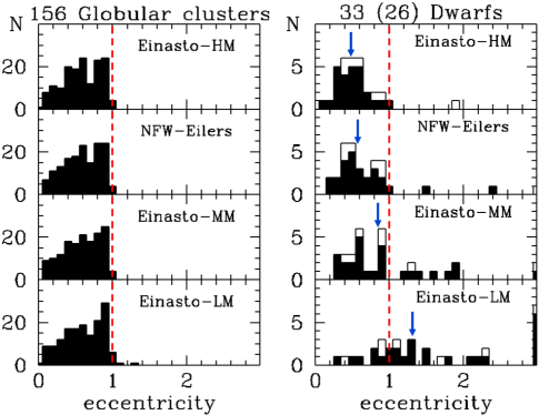
Figure 1: Histograms of the eccentricity distribution of GCs (left) and dwarf galaxies (right) for four MW mass models (decreasing total mass from top to bottom) that are consistent with the MW rotation curve (Jiao et al., 2021). Open and filled histograms represent all the 33 dwarfs, and a subsample of 26 of them having their internal velocity dispersion measured. The blue arrows in the right panels indicate the median eccentricities of 0.478, 0.581, 0.829, and 1.301 from the top to the bottom. The vertical red-dashed line delimits ecc=1.

Figure 1 shows how the orbital eccentricity depends on the MW mass models. The distribution of eccentricities of 156 GCs is very stable when decreasing the MW mass from 15 to $5.1\times 10^{11}\,{\rm M}_{\sun}$, i.e., all of them follow elliptical and bound orbits. It is only by adopting the smallest MW mass ($2.8\times 10^{11}\,{\rm M}_{\sun}$) that the Pyxis and Terzan 8 orbits becomes hyperbolic (ecc=1.3 and 1.07, respectively), while the orbits of three other GCs (Pal 3, Eridanus, and Arp 2) have eccentricities just below 1.

This contrasts with the net increase of dwarf eccentricities when the MW mass decreases, from the top to the bottom right panels of Figure 1. Dwarf galaxies show a smaller median eccentricity than that of GCs for high MW mass models, while two-thirds of them are on hyperbolic orbits for the lowest MW mass model (Einasto_LM). Table LABEL:tab:ecc of Appendix B gives dwarf eccentricities for each of the four adopted MW mass models of Table 1.

Figure 1 illustrates that by using GCs to characterize the MW mass, one would find values close or larger than that of the Einasto-MM model (e.g., see Wang et al. 2022 and references therein). If considering dwarfs as MW satellites, one would automatically derive large masses for the MW, which suggests that MW mass determinations are strongly affected by the choice of adopted priors. It implies that the total dynamical mass of the MW derived from the Gaia DR2 rotation curve (Eilers et al., 2019; Jiao et al., 2021) is still an unknown within a large range of values.

Another illustration of the impact of the MW mass choice is given by the determinations of the infall time for MW dwarfs. According to Boylan-Kolchin et al. (2013), satellites with the most recent infall have the largest orbital energy (or the smallest binding energy), which is well illustrated in Figure 1 of Rocha et al. (2012). This follows the expectations of the onion skin model of Gott (1975). It has prompted many studies (Rocha et al., 2012; Fillingham et al., 2019; Miyoshi & Chiba, 2020; Barmentloo & Cautun, 2023) to use dedicated zoomed simulations to directly compare MW dwarfs with simulated satellites. If considering large MW masses, dwarf galaxies would have smaller energy than objects near the escape velocity lines, which unavoidably leads to large infall lookback times, as found by the above studies that considered $M_{\mathrm{tot}}/(10^{11}\,{\rm M}_{\sun})$= 19, 10-25 (average 17 from the ELVIS suite, Garrison-Kimmel et al. 2014), 15.4, and 10-20, respectively. Right panels of Figure 1 show that by decreasing the MW mass below this range, more and more dwarfs become unbound, leading to small infall lookback times. It suggests that the inferred infall time is thus dependent on what total MW mass has been assumed.

This is why, in Paper I and in this paper, we have adopted a different approach by estimating only relative infall times, after comparing MW dwarf orbital energies to robust estimates of the infall times for past merger events in the MW (Kruijssen et al., 2020; Malhan et al., 2022), i.e., independently of the MW mass. Our constraints on the MW dwarf infall time are coming from a comparison with assumed Gaia-Sausage-Enceladus (8-10 Gyr ago), and Sgr (4-6 Gyr ago) infall times. Since the orbital energy of MW dwarfs are larger than that of the latter events, their infall epochs are expected to be more recent (see Figure 6 of Paper I).

In the following we will try to identify which relationship between intrinsic and orbital properties is independent on the MW mass model, either for dwarfs or for GCs.

3 Globular cluster properties

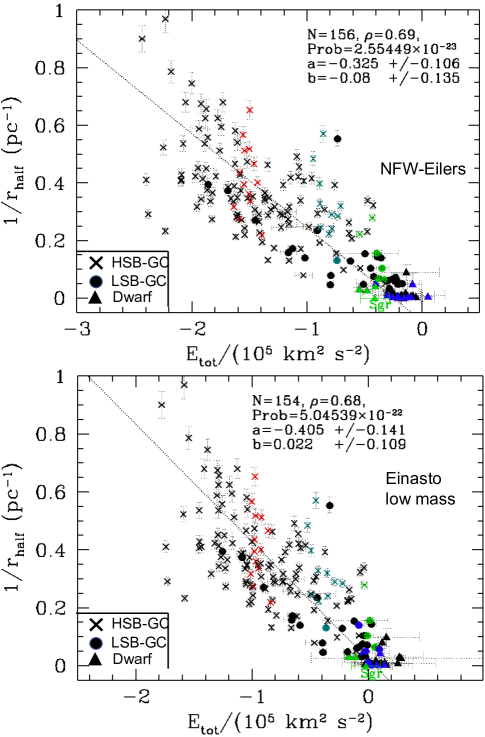
Figure 2: Inverse of the half-light radius versus total orbital energy, for HSB-GCs (crosses), LSB-GCs (full dots), and dwarfs (triangles). Identified structures by Malhan et al. 2022 and Kruijssen et al. 2020 are represented by different color codes (Kraken: red; Gaia-Sausage-Enceladus: cyan; Sgr: green). Dwarf galaxies and LSB-GCs belonging to the VPOS (Pawlowski et al., 2012) are shown with blue colors. The top (bottom) panel shows 156 (154) GCs and 33 dwarfs after calculating the total energy from the NFW (Einasto-low mass) model of the MW. The location of Sgr is indicated by a green triangle. The dotted line shows the fit of the GC points, and the corresponding slope (a) and rest (b), as well as the significance of the Spearman rank correlation are given on the top-right of each panel. One sigma error bars on orbital quantities such as pericenter and total energy are based on Monte Carlo calculations assuming Gaussian distributions for PM and radial velocity errors.

3.1 The correlation between half-light radius, pericenter radius and total energy

In Paper I, we have shown that the half-light radius scales as the inverse of the total orbital energy ($E_{\rm tot}$) for the NFW model of the MW (Eilers et al., 2019; Jiao et al., 2021, see also Table 1). Figure 2 illustrates that this anti-correlation trend is highly significant (probability of a coincidence smaller than $10^{-20}$). We have tested the slope of the logarithmic relation between $r_{\rm half}$ and $E_{\rm tot}$ for the 4 MW mass models of Table 1, which ranges from –1.1$\pm$0.3 to –1.18$\pm$0.3. We then adopt $-1$ for simplicity, i.e., $E_{\rm tot}$ $\propto$ 1/$r_{\rm half}$ in Figure 2. It shows that the GC size depends on the number of previous passages at pericenter, and that smaller stellar systems are associated to early infall into the MW (see Paper I). This relation does not depend on the MW model as it is illustrated by comparing top and bottom panels of Figure 2, for which GCs share very similar locations. Figure 2 also illustrates how identified structures (see colored points) have almost a single energy value, suggesting the relation between their formation epoch and the energy described in Paper I.

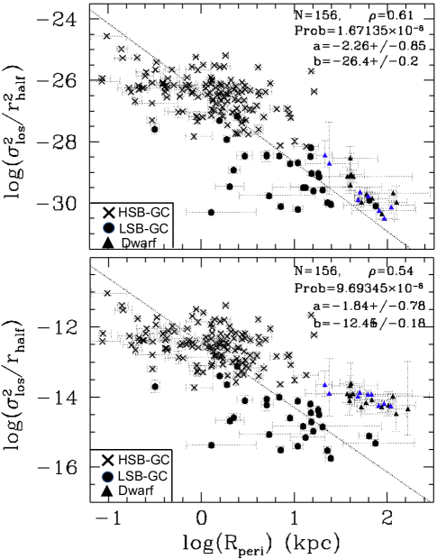
Figure 3: $\sigma_{\rm los}^{2}r_{\rm half}^{2}$ (proportional to a 3D density) and $\sigma_{\rm los}^{2}r_{\rm half}$ (proportional to a surface density) of GCs versus $R_{\rm peri}$. Same symbols than for Figure 2, except that here only VPOS dwarfs have kept their (blue) color. One sigma error bars on orbital quantities such as pericenter and total energy are based on Monte Carlo calculations assuming Gaussian distributions for PM and radial velocity errors.

For GCs we adopt the same relation as Baumgardt (2017) between the dynamical mass (or total mass inside $r_{\rm half}$) and the velocity dispersion and the half-light radius, which has been established by Wolf et al. (2010), under the assumption of self equilibrium and constant line of sight velocity dispersion:

$$\frac{M_{\rm tot}(r_{\rm half})}{1\,{\rm M}_{\sun}}=930\,\left(\frac{\sigma_{\rm los}}{1\,{\rm km\,s}^{-1}}\right)^{2}\,\left(\frac{r_{\rm half}}{1\rm pc}\right)\ ,$$ (3)

where $\sigma_{\rm los}$ has been estimated within $r_{\rm half}$.

By dividing the total mass by $r_{\rm half}^{2}$ and by $r_{\rm half}^{3}$, one obtains quantities proportional to the averaged surface density $\Sigma_{\rm tot}\propto\sigma_{\rm los}^{2}/r_{\rm half}$ and to the 3D density ($\rho_{\rm tot}\propto\sigma_{\rm los}^{2}/r_{\rm half}^{2}$) inside $r_{\rm half}$, respectively. Figure 3 shows how the two latter quantities depend on pericenter. The resulting anti-correlations (see straight-dotted lines) are not unexpected for GCs. We have shown that their pericenter (and angular momentum) is well correlated with their energy (see Paper I), while Figure 2 shows how the energy correlates with the half-light radius. The latter correlation is likely responsible for the strong, but quite scattered relation between surface-density and 3D-density with pericenter.

Figure 4 shows how slope, correlation significance, and probability are changing with X when considering the relation between $\sigma_{\rm los}^{2}\,r_{\rm half}^{X}$ and $R_{\rm peri}$ for 156 GCs. For $X=1$, the former represents the total mass that barely correlates with $R_{\rm peri}$, while the anti-correlation coefficient ($\rho$) increases for increasing $|X|$. This is expected because the pericenter should be directly related to the orbital energy (see Paper I), which is proportional to the half-mass radius (see Figure 2), so the velocity dispersion should be a more minor factor.

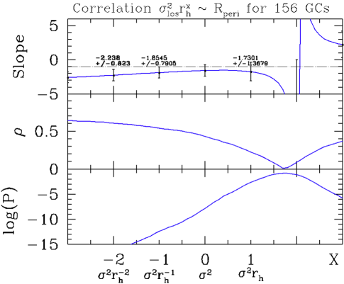
Figure 4: Slope, correlation $\rho$ (its absolute value), and associated probability (in logarithmic scale) of the correlation between $\sigma_{\rm los}^{2}r_{\rm half}^{X}$ and $R_{\rm peri}$ for $X$ (in abscissa) taking values from $-3$ to +3. Each quantity is shown on the $X$ axis. The NFW model has been assumed for calculating $R_{\rm peri}$, but curves for other models cannot be distinguished from it.

3.2 How tidal shocks affect an orbiting stellar system

Tidal shocks exerted on GCs near their pericenter have been theoretically described for orbits passing close to the bulge or through the disk (Aguilar et al., 1988; Gnedin & Ostriker, 1999). Aguilar et al. (1988) showed that the average energy increase of a star after integrating over the whole GC has been calculated to be:

$$\Delta E=\frac{4}{3}\,\eta\left({GM_{\rm MW}(R_{\rm peri})\over R_{\rm peri}^{2}}\right)^{2}\,\left({r_{\rm rms}\over V_{\rm peri}}\right)^{2}\,,$$ (4)

where $V_{\rm peri}$ is the velocity at pericenter, $\eta$ is a dimensionless parameter that accounts for our lack of understanding of the details of the tide (deviations from the impulsive approximation), and:

$$r_{\rm rms}^{2}=3\,r_{\rm half,3D}^{2},$$ (5)

with:

$$r_{\rm half,3D}=\frac{4}{3}r_{\rm half},$$ (6)

the latter comes from Wolf et al. (2010) after transforming the theoretical $r_{\rm half,3D}$ into the observed $r_{\rm half}$ calculated from the stellar surface density. The problem with the rms radius is that it may diverge for models whose outer density slope is $>-5$ (including the Plummer model, often used to represent the density profiles of GCs). Only the King (1966) model and truncated models would have finite rms radius. One possibility is to limit the calculation of the rms radius to the bound particles.

One extreme case is tidal disruption, where, to first order, the energy impulse per unit mass from the MW tide matches the binding energy per unit mass $3/2\sigma^{2}$, where $\sigma$ is the average one-dimensional velocity dispersion of the system (but see van den Bosch et al. 2018 for a more detailed analysis that shows the resilience of stellar systems to tides). Then, one can combine Eqs. 4,  5, and  6, yielding:

$$\frac{\sigma^{2}}{r_{\rm half}^{2}}={128\over 27}\,\eta\left({g_{\rm MW}(R_{\rm peri})\over V_{\rm peri}}\right)^{2},$$ (7)

where $g_{\rm MW}(R_{\rm peri})$= $GM_{\rm MW}(R_{\rm peri})/R_{\rm peri}^{2}$ is the gravitational acceleration exerted by the assumed spherical MW at $R_{\rm peri}$. Values of $\rm g_{\rm MW}$ and of $V_{\rm peri}$ have been derived from Monte Carlo realizations assuming Gaussian distributions for PM and radial velocity errors. These calculations are based on galpy (Bovy, 2015), to warrant a correct propagation of errors as well as to consider effects related to axisymmetric disks. However, Eq. 7 corresponds to the specific and extreme case when the energy impulse per unit mass equals the binding energy per unit mass. In the following, we generalize it by considering cases for which the energy impulse only amounts to a fraction $f$ of the binding energy, which applies to many systems that can be affected by tides, but not fully destroyed by them. To simplify, $f$ also accounts for $\eta$, and the latter can shrink below 1 (see Fig. 3 of Aguilar et al. 1988). This leads to:

$$\frac{\sigma^{2}}{r_{\rm half}^{2}}\times f\,={128\over 27}\,\left({g_{\rm MW}(R_{\rm peri})\over V_{\rm peri}}\right)^{2}.$$ (8)

Eq. 8 compares structural (left) with orbital (right) quantities, which is illustrated in Figure 5, in which we have assumed $\sigma=\sigma_{\rm los}$ in spherical symmetry, a condition that is verified for most GCs. Eq. 8 accounts for bulge and disk shocks, which are both described by the same formulae, though with different timescales.

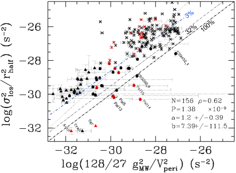
Figure 5: Correlation between internal GC properties ($\sigma_{\rm los}^{2}r_{\rm half}^{2}$, proportional to 3D density) and external properties from tidal shock theory for a GC (Aguilar et al., 1988; Gnedin & Ostriker, 1999) passing near pericenter to be disrupted (see Eq. 8). Same symbols as in Figure 2, but now indicating in red color the GCs associated to a tidal tail (Zhang et al., 2022, see their Table 3). Dot-dashed lines correspond to the equality , $f=1$ (thick), to $f=0.32$ (thin) and to $f=0.032$ (blue), respectively, the latter being almost confused with the dotted line that represents the correlation for GCs. All quantities in the abscissa have been extracted at $R_{\rm peri}$.

The left hand of Eq. 8 corresponds to the square of the inverse crossing time

$$t_{\rm cross}={r_{\rm half}\over\sigma}$$ (9)

for a star inside a stellar system, while the right hand estimates the inverse-square of a time ($t_{\rm perturber}$) linked to the perturber passage, i.e., the MW. In the case of a fast perturber, $t_{\rm shocks}\leq t_{\rm cross}$ and the impulse approximation may apply (Aguilar & White, 1985; Gnedin & Ostriker, 1997), implying that stellar systems found below the equality line in Figure 5 are likely tidally shocked, disrupted, or stripped. In such a case, the energy brought by tidal shocks becomes equal or larger than the kinetic energy necessary to balance the self-gravity of the stellar system, which becomes dominated by tides.

One would expect that such stellar systems may show tidal tails. Red symbols in Figure 5 indicate GCs for which such tail systems have been identified (Ibata et al., 2021; Zhang et al., 2022, see their Table 3), although these surveys cannot be considered as complete since not all GCs have been scrutinized for tidal tail search.

3.3 The different properties of HSB and of LSB-GCs

Figure 5 reveals large differences when comparing HSB with LSB-GCs. HSB-GCs appear much more robust against tides, since none (among 127) are below the equality line $f$= 100%. It contrasts with the 7 (24 %) LSB-GCs that lie well below the line. Most of the latter possess a known system of tidal tails (4 among 7), while tails are less frequent for LSB-GCs above the line (4 among 22). This furthermore contrasts with HSB-GCs, for which all systems possessing tidal tails are well above the equality line, and even above the $f$= 0.32 line.

Figure 5 shows that quantities at both sides of Eq. 8 correlate well (156 GCs, $\rho=0.62$, $P=1.4\times 10^{-9}$). Here we show that it is due to the fact that both quantities anti-correlate with the pericenter. According to the top panel of Figure 3, $\sigma_{\rm los}^{2}/r_{\rm half}^{2}$ evolve as $R_{\rm peri}^{-2.26}$. Most HSB-GCs have their orbits within 15 kpc, for which $M_{\rm MW}$ $\propto$ R (see, e.g., Jiao et al. 2021), and then $g_{\rm MW}$=$GM_{\rm MW}/R^{2}$ $\propto$ $R^{-1}$, and we also find (see Appendix LABEL:sec:Vperi) that $V_{\rm peri}$ is almost independent to $R_{\rm peri}$. It lets the second hand of Eq. 8 following to $R_{\rm peri}^{-2}$. In other words, stellar systems have decreasing pericenter, orbital energy, and half light radii from the left to the right of Figure 5.

HSB-GCS density increases by $\sim$ 3% at each pericenter passage (Martinez-Medina et al., 2022, see their Fig. 9), a phenomenon which is called star evaporation (Binney & Tremaine, 2008). Lying on the top-right of Figure 5, they are experiencing much more pericenter passages than other stellar systems. In Figure 5 their median location is very close to expectations for $f$= 0.03 (see the blue dot-dashed line), which means that they are stellar systems in pseudo equilibrium with the MW potential and tides. This explains why only few of them possess tails. Because they orbit at low radii, many different processes could generate these tails, such as gravitational interactions with other substructures, e.g., giant molecular clouds, spiral arms, and the bar (Ibata et al., 2021, and references therein).

This contrasts with LSB-GCs that appear more fragile due to their much lower densities (300 times on average, see Figure 5), while at significantly larger pericenters, i.e., their orbits may extend to regions far from the MW disk. 24% of them are fully tidally shocked, and they are more affected by tides than HSB-GCs, since their locations in Figure 5 are generally well below the $f$= 0.03 line. Conversely to HSB-GCs, their passages to pericenter are relatively rare, and then their properties are not fully shaped by the MW potential, yet.

HSB-GCs are in pseudo equilibrium with the MW potential. Going further to the bottom-left of Figure 5, one finds LSB-GCs that are much less at equilibrium. In the next section we examine whether or not dwarfs galaxies that lie at the very bottom-left of Figure 5 are in equilibrium.

We have verified that all the above properties, including the relative locations of both GCs and dwarf galaxies relatively to the equality line in Figure 5, do not change with the MW potential.

4 Dwarf galaxy properties

4.1 Comparison of dwarf galaxy and LSB-GC properties

Figure 5 shows that LSB-GCs have more similarities in the investigated properties with dwarf galaxies (full triangles) than with HSB-GCs. First, both populations show a fraction of fully tidally disrupted systems, i.e., those below the equality line in Figure 5. The three dwarf galaxies below the equality line are Sgr, Crater II and Antlia II. The first is well-known for its gigantic system of tidal streams that surround the MW (Ibata et al., 2001), and the other two, by their extremely low stellar density and large sizes. Antlia II is likely associated with tidal tails, which is also suspected for Crater II (Ji et al., 2021; Wang et al., 2023, hereafter Paper III). Second, two LSB-GCs (Pal 3 and Crater) lie in the sequence delineated by dwarfs in Figure 5. This corroborates Marchi-Lasch et al. (2019) conclusions that structural properties of ultra faint dwarfs and of low surface brightness GCs could be rather similar.

However, none of the 24 remaining dwarfs that lie above the equality line show tidal tails (Hammer et al., 2020), while some LSB-GCs do. In addition, most dwarf galaxies do not show a spherical morphology, and their surface brightness are generally fainter than that of LSB-GCs.

4.2 A strong anti-correlation between structural and orbital dwarf properties

In Figure 5, 24 of the 26 dwarf galaxies appear at first glance to be unaffected by MW tidal shocks due to their location well above the equality line and the absence of tidal tails. However, one may wonder why they delineate a sequence that is precisely parallel and offset by $\sim$ +1.5 dex to the equality line, with a significance of $\rho=0.66$ ($P=8.6\times 10^{-4}$). The same applies after examining the two panels of Figure 3 where dwarf densities correlates with $R_{\rm peri}$ as well as GCs, though being offset from them. To understand this, we propose to examine the core sample of 24 dwarf galaxies obtained after removing Antlia II and Crater II. In the following, we investigate which combination of their intrinsic properties (e.g., $r_{\rm half}$, $\sigma_{\rm los}$, and $L_{V}$) correlates the best with orbital properties (e.g., their pericenter, $R_{\rm peri}$).

Since tidal forces scale with distance to the system center, and that dark matter is more extended than stars, one expects that dark matter can be used to measure the strength of the tides within dwarf galaxies. We propose to use the dark matter contribution to the stellar velocity dispersion as the test for tidal theory, and vice-versa. Its squared value is:

$$\sigma_{\rm DM}^{2}\approx\sigma_{\rm los}^{2}-\sigma_{\rm stars}^{2}\ ,$$ (10)

where $\sigma_{\rm stars}$ is the contribution of stars to the stellar velocity dispersion (the formula is an approximation because of the neglect of the gas component, which appears justified for MW dwarf galaxies). We measure the contribution of the stars to the velocity dispersion, $\sigma_{\rm stars}\equiv\sigma_{\rm ap}(R)$, in a cylindrical aperture of radius $R$ by integrating over the cylinder the stellar contribution to the radial velocity dispersion of the stars, itself found by integrating the Jeans equation of local dynamical equilibrium assuming further isotropic kinematics. This quantity involves a triple integral (one for solving the Jeans equation for the radial component of the 3D velocity dispersion, one for integrating along the line of sight, and one for integrating over the different lines of sight within the aperture). We use the single integral exact expression of equation (B7) of Mamon & Łokas (2005), corrected in Mamon & Łokas (2006), valid for systems with isotropic velocities

$$\sigma_{\rm stars}^{2} \equiv\sigma_{\rm ap}^{2}(R)$$

$$={4\pi\,G\over 3\Sigma(R)}\,\left[\int_{0}^{\infty}r\nu(r)M(r)\,{\rm d}r\right.$$

$$\qquad\qquad\quad\left.-\int_{R}^{\infty}{(r^{2}-R^{2})^{3/2}\over r^{2}}\nu(r)\,M(r)\,{\rm d}r\right]\ ,$$ (11)

where $\nu(r)$ and $\Sigma(R)$ are the 3D and surface stellar number density profiles, respectively, while $M(r)$ is the total mass profile. Figure 6 gives an example for Fornax, assumed to be embedded in a DM halo.

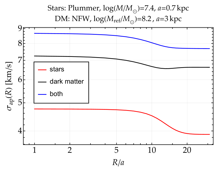
Figure 6: Contribution of stars and dark matter to the velocity dispersion measured in a cylindrical aperture, i.e. the average los velocity dispersion, for a dwarf such as Fornax. Here, $M_{\rm ref}=M_{\rm DM}(a_{\rm dark})$, and isotropic velocities are assumed.

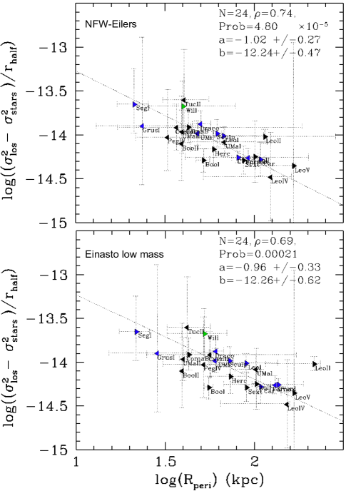
Figure 7: Free-fall tidal shocks (or DM) acceleration (in km $\rm s^{-2}$) based on dSph kinematics (($\sigma_{\rm los}^{2}-\sigma_{\rm stars}^{2})\,r_{\rm half}^{-1}$) versus pericenter radius. Data ($\sigma_{\rm los}$, $L_{V}$, $r_{\rm half}$) come from Table LABEL:tab:struct of Appendix B.

The top panel of Figure 7 shows that when removing quadratically $\sigma_{\rm stars}$ the correlation reaches a slightly higher significance, i.e., $\rho=0.74$ between ($\sigma_{\rm los}^{2}-\sigma_{\rm stars}^{2})/r_{\rm half}$ and $R_{\rm peri}$, which is associated to a low probability that it occurs by chance, $P=4.8\times 10^{-5}$.

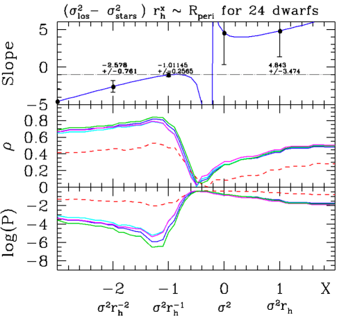
Figure 8: Slope, correlation $\rho$ (its absolute value), and associated probability (in logarithmic scale) of the correlation between $(\sigma_{\rm los}^{2}-\sigma_{\rm stars}^{2})$ $r_{\rm half}^{X}$ and $R_{\rm peri}$ (red-dashed line: with $R_{\rm GC}$) from $X=-3$ to $X=2$. Each quantity is shown on the $X$ axis, and $\rho$, and associated probability are given for the 4 MW mass models (see colored lines).

Figure 8 shows how slope, correlation significance, and probability are changing with X when considering the relation in logarithmic scale between ($\sigma_{\rm los}^{2}-\sigma_{\rm stars}^{2})\,r_{\rm half}^{X}$ and $R_{\rm peri}$ for 24 dwarf galaxies. It shows that the correlation peaked at $X=-1$, which likely drives all correlations at $X<-1$.

Anti-correlations shown in Figures 3,  7, and  8 between by dwarf galaxy structural and orbital parameters have already been identified by Hammer et al. (2019), who also considered $\sigma_{\rm los}^{2}-\sigma_{\rm stars}^{2}$, and by Kaplinghat et al. (2019), who found robust anti-correlations between 3D density within 150 pc and pericenter (see their fig. 2). However, Kaplinghat et al. (2019) found that the anti-correlation vanishes for ultra-faint dwarfs (UFDs). This difference can be explained because, in contrast to us, they include both Antlia II and Crater II in the UFD sample, and both objects dominate the relation because of their extremely low densities (see their Fig. 3). We re-assess that Antlia II and Crater II (as well as Sgr) are experiencing strong tidal stripping conversely to the rest of the 24 dwarfs considered here, as it is shown in Figure 5. We confirm the Kaplinghat et al. result, i.e., by inserting Antlia II and Crater II in Figures 3,  7, and  8 is sufficient to wash out the anti-correlation, because they have densities several dex lower than those of other dwarfs.

If MW dwarf galaxies were at self-equilibrium with their own gravity, both $(\sigma_{\rm los}^{2}-\sigma_{\rm stars}^{2})/r_{\rm half}$ and $(\sigma_{\rm los}^{2}-\sigma_{\rm stars}^{2})/r_{\rm half}^{2}$ would correspond to the surface and 3D mass densities of the sole dark matter (DM) component. Looking at the slope of the correlations (see top panel of Figure 8), it implies that both quantities vary as $R_{\rm peri}^{-1}$ and $R_{\rm peri}^{-2.6}$, respectively. If dwarf galaxies were long-term satellites of the MW, this could be interpreted as being caused by a ’survivor bias’, i.e., satellites with small pericenter would be those having been shielded against the tidal forces (see Vitral & Boldrini 2022), which means that they have to be denser (Kaplinghat et al., 2019), even favoring cusped density profiles in their center (Errani et al., 2023). Assuming that MW dwarfs are long-term satellites, Robles & Bullock (2021) found that subhalos with small pericenters are indeed denser after a Hubble time evolution, while Kravtsov & Wu (2023) did not.

However, due to their high orbital energy and angular momenta, most dwarf galaxies are stellar systems that arrived late in the MW halo (less than 3 Gyr ago, see Paper I). It results that they have no time to make one or few orbits in the MW halo, in sharp contrast with a long-term satellite hypothesis. It thus appears quite enigmatic why their structural parameters such as $r_{\rm half}$ and $\sigma_{\rm los}$ show a correlation with orbital parameters in Figure 7 and with the tidal-shock characteristic time in Figure 5.

5 Discussion

5.1 Dwarf galaxies with escaping stars affected by MW tides

Figure 8 also shows that the correlations with pericenter ($R_{\rm peri}$) are much stronger than with galactocentric radius ($R_{\rm GC}$, red line). This suggests that intrinsic properties of dwarf galaxies are linked to MW tides (see also Sect. 5.3 for a more detailed discussion). This calls for a mechanism related to the expected progenitor properties of MW dwarfs, a few Gyr ago. Sect. 5.7 discusses the impact of a dwarf recent infall onto their DM properties.

Beyond 300 kpc, all dwarfs (but a few, e.g., Cetus and Tucana) are gas-rich, while they are gas-poor within 300 kpc (except the massive LMC/SMC; Grcevich & Putman 2009). If the former are progenitors of the latter, gas-rich dwarfs are expected to be stripped during their infall due to the ram pressure caused by the Galactic halo gas (Mayer et al., 2006). The role of the removed gas during the process could be essential, if it induces a lack of gravity implying that many stars have to expand (Grishin et al., 2021) following a spherical geometry (for an isotropic distribution of initial velocities of stars). The fraction of stars that are lost depends on the total initial mass, on the mass fraction initially represented by the gas, and also on the relative size of the different components in the progenitor.

Simulations performed by Yang et al. (2014) have shown that when the gas is lost near the pericenter passage, it increases the dwarf kinematics, because many stars are escaping the system and are then affected by the MW gravity. Hammer et al. (2020) proposed an ideal case for which a fraction ($f_{\rm ff}$, ff standing for free-fall) of stars are not affected by the dwarf self-gravity, but by the MW gravity. Assuming a Plummer profile for the dwarf, they calculated that the dwarf squared velocity dispersion is increased by:

$$\Delta\sigma^{2}=2\sqrt{2}\,g_{\rm MW}\,r_{\rm half}\,f_{\rm ff},$$ (12)

where $g_{\rm MW}$ stands for the MW gravity. Equation 12 is over-simplified since in reality, stars lying in the center may move sufficiently fast that they are adiabatically invariant to the actions of the moving MW gravitational field (Weinberg, 1994; Binney & Tremaine, 2008). Some of our simulations (Paper III) show a residual core that appears stable against star expansion and MW gravity. This is an adiabatic effect, since the most bound stars have very short orbital periods compared to the timescale of the MW flyby. So, for the encounter, they appear smeared along their internal cluster orbits, and the external perturbation can only kick the orbit as a whole (i.e. mainly linear momentum exchange). For the cluster envelope stars, the flyby is impulsive, they only cover a fraction of its orbits during the flyby, so the external perturbation can do work deforming their orbits (i.e. mainly energy exchange), heating up their dynamics and contributing to their expansion and eventually becoming unbound.

The consequence would be to change $f_{\rm ff}$ in Equation 12 into a smaller value if stars within $r_{\rm half}$ are less affected due to adiabatic invariance. Simulations also show that the gas removal is a turbulent process that affects both gas and star motions during the time they are bound together, and also affect the velocity dispersion of stars after gas removal. In the following, we consider this to be accounted for by the $f_{\rm ff}$ factor, which depends also on the structural properties of the dwarf. We derive:

$${\sigma_{\rm los}^{2}-\sigma_{\rm stars}^{2}\over r_{\rm half}}=2\sqrt{2}\,g_{\rm MW}\,f_{\rm ff},$$ (13)

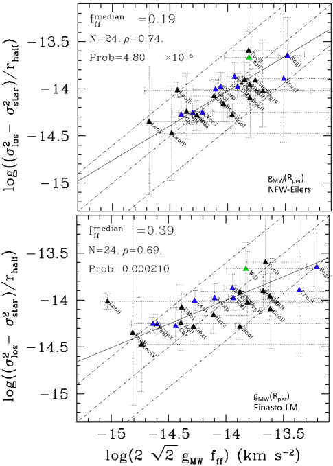
Figure 9: Free-fall tidal shocks (or DM) acceleration (in km $s^{-2}$) based on dSph kinematics (($\sigma_{\rm los}^{2}-\sigma_{\rm stars}^{2})/r_{\rm half}$) versus MW gravity at pericenter, for the NFW (top panel) and Einasto low mass (bottom panel) MW models. The solid line represents the best fit of the correlation, whose characteristic numbers are provided in the top-left. The line corresponding to the median of $f_{\rm ff}$ is the central dot-dashed line, while the two other dot-dashed lines correspond to the median value, multiplied (top line) or divided (bottom line) by 2.5, respectively.

Figure 9 shows that ($\sigma_{\rm los}^{2}-\sigma_{\rm stars}^{2})$/$r_{\rm half}$ correlates well with the MW gravity, with a similar correlation strength than that with pericenter. For the NFW MW mass model (top panel) tidal shocks exerted on expanding stars can reproduce the observations if the fraction ($f_{\rm ff}$) of the latter ranges from 0.08 (bottom dot-dashed line) to 0.48 (top dot-dashed line), with a median at 0.19. Classical dwarfs, but Leo II, are mostly near the median value, as well as most dwarfs of the VPOS (blue triangles, see, e.g., Pawlowski et al. 2012), but Grus I.

When adopting the low MW mass model (bottom panel of Figure 9), $f_{\rm ff}$ ranges from 0.16 to 0.98, with a median value of 0.39. However, Leo II appears as an outlier ($f_{\rm ff}$ $>$ 1), which could be caused by the quite large uncertainty on the MW acceleration at pericenter, or alternatively, because it does not obey Eq. 13.

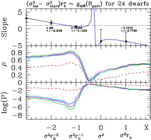
Figure 10: Slope, correlation $\rho$, and associated probability (in logarithmic scale) of the correlation between $(\sigma_{\rm los}^{2}-\sigma_{\rm stars}^{2})$ $r_{\rm half}^{X}$ and $\rm g_{MW}$ at $R_{\rm peri}$ (red-dashed line: at $R_{\rm GC}$) from $X=-3$ to $X=2$, respectively. Each quantity is shown on the $X$ axis, and associated probability are given for the 4 MW mass models (see colored lines).

Figure 10 confirms our finding (see Figure 8) that the correlation with $g_{\rm MW}$ is driven by $X=-1$, which supports the validity of Eq. 13, and then the fact that intrinsic properties such as $\sigma_{\rm los}$ and $r_{\rm half}$ are changing through a temporal sequence, gas removal, star expansion, and then MW tidal shocks. It also shows that the correlation is much improved when adopting MW gravity at pericenter (see the red-dashed line representing gravity at $R_{\rm GC}$), suggesting further a tidal origin for the observed correlations.

We notice that Figure 10 is essentially similar than Figure 8 probably because in the range of pericenter values, $g_{\rm MW}$ values are simply set by $R_{\rm peri}$ values. However, it provides a good test for the validity of Eq. 13.

5.2 Comparison with numerical simulations

A physical interpretation of the correlation shown in Figure 9 may need two conditions to be fulfilled at the time dwarfs are observed:

1. Due to the gas removal and gravity loss a significant fraction of stars are expanding to the dwarf outskirts and are gradually less affected by the dwarf gravity;

2. Gas loss happened at a time quite close from that of the pericenter passage, which resulted in many of the stars in the dwarf outskirts to be tidally shocked by the MW.

The first condition is fulfilled if the gas represents $\sim$50% of the baryonic mass within the initial half-mass radius of the dwarf progenitor. For example, such a condition is well reached for the dwarf irregular WLM (Yang et al., 2022b) that has a stellar mass similar to that of Fornax (McConnachie, 2012). The second condition is likely reached because there is a significant excess of dwarf spheroidal and ultra-faint dwarfs lying near pericenter (Fritz et al., 2018; Hammer et al., 2020; Li et al., 2021), where both ram pressure and tidal forces are maximal.

Simulations by Yang et al. (2014) have shown that their initial dwarf 3 is able to reproduce the flat velocity dispersion radial profiles of UMi or Draco. It also reproduces morphologies and surface-brightness of the two dwarfs (see also Figs. 10 and 11 of Hammer et al. 2018b). In these simulations a significant part of the initial stars has been lost during the dwarf infall in the MW halo, due to their expansion after gas removal.

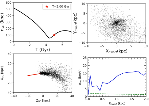
Figure 11: Evolution of stars in a hydrodynamical simulation made in Paper III and based on a MW mass model of $8\times 10^{11}$ $\,{\rm M}_{\sun}$, with a halo gas mass density following that has been adopted by Wang et al. (2019) to reproduce the Magellanic stream. In this simulation the dark matter halo is truncated at $r_{200}=189\,\rm kpc$. Top-left panel gives the trajectory of the dwarf (Galactocentric distance versus time) that follows that of Sculptor, whose star properties are captured 0.5 Gyr after pericenter passage (see the red point in the top-left panel). Top-right panel indicates that a significant fraction of stars have left the main body of the dwarf while bottom-left panel shows that it brings an additional extended component mostly along the line of sight (indicated by the red arrow). Bottom-right panel shows the radial profile of the line-of-sight velocity-dispersion similarly to measurements currently made for MW dwarfs (blue solid line) and compare it to expectations from equilibrium with its stellar mass content (green dash line). More details will be given in Paper III.

More simulations are needed to verify whether each MW dwarf can be reproduced in this way, including the more massive ones, e.g., Sculptor (see Paper III), as well as ultra-faint dwarfs. One difficulty is numerical, e.g., it is essential to ensure a high resolution and thus small mass for the stellar and gas particles in the dwarfs, the latter of which have to interact with MW hot gas particles, the total mass of which is a hundred to a thousand times larger than that of the initial dwarfs. Comparison between simulations and observations needs to consider all stellar particles, including those that are just in projection on the dwarf core since they also contribute to $\sigma_{\rm los}$ (see, e.g., bottom-left panel of Figure 11).

Simulations of Paper III show that if the above conditions (i), and (ii) are granted, the velocity dispersion (bottom-right panel of Figure 11) is much higher than expectations from self-equilibrium of the stellar component alone (compare the dashed green line with the solid blue line). This increase is found maximal at pericenter passage (T$\sim$ 4.5 Gyr, see top-left panel of Figure 11), while such a phenomenon has a duration of several hundred of million years. This is indicated by Figure 11 that represents the stellar particle properties at T= 5 Gyr (see the red star in the top-left panel), when velocity dispersion is still considerably increased (compare blue solid and green dash lines in bottom-right panel). This additional velocity dispersion is provided by stars unbound to the dwarf, which are affected by tidal shocks as expected from Eq. 9. The situation in the central core of the dwarf is probably more complex, since $\sim$300 Myr after the gas release, there are still stars that are in expansion because of their large velocity, while some other core stars can also be affected by tidal shocks since their small velocity may place them in the impulse approximation conditions.

5.3 Combination of tidal shocks and ram-pressure stripping

Figure 11 also illustrates that Equation 13 is too simplistic in assuming that all the energy exchange ($\Delta E=\sigma^{2}$/2) occurs only along the line of sight, especially if the main contribution occurs at pericenter. In reality, the exchange of energy should result from an integration over all the past orbit of the dwarf galaxy. It would affect the validity of Equation 13 especially for nearby dwarf galaxies, for which the direction of $g_{\rm MW}$ when calculated at pericenter may differ from the line-of-sight. This could explain why the correlation slope in Figure 9 is smaller than 1, i.e., because the X-axis value could have been overestimated for nearby dwarfs, such as Segue I or Grus I that lie on the right of the Figure.

Another limitation of Equation 13 is that in addition to MW tidal shocks, gas removal also leads to an increase of the dwarf velocity dispersions. This is because after gas loss, stars keep the memory of their initial velocity dispersion, which is large because it balanced the initial total mass of both gas and stellar components. Since ram pressure stripping is also expected to be maximal near pericenter, it could contribute to the correlations found in Figures 7 and  9, in addition to tidal shocks described by Equation 13.
Paper III shows that this could explain the larger velocity dispersion of Antlia II when compared to that of Crater II. The latter, having not passed its pericenter, is mostly affected by the gas removal, while the former, having passed its pericenter, is furthermore affected by tidal shocks. Reproducing the excess of velocity dispersion in all dwarfs, including ultra-faint dwarfs, would require a specific modeling of each of them. Besides numerical limitations discussed above, this is also complicated by the fact that new observations from deeper surveys (e.g., from Cantu et al. 2021 and Chiti et al. 2022) have shown that structural parameters such as the half-light radius of Grus I may have changed from 28 to 151 pc. On the other hand, ultra-faint dwarf orbits often have larger eccentricity than classical dwarfs, which suggests a better efficiency of MW tidal shocks.

5.4 Consistency of dwarf infall times with their star formation histories

A scenario for which MW halo gas and gravity has recently shaped the dwarf morphologies and kinematics differs with results of many previous studies, for which constraints about infall times of MW dwarf galaxies were mostly coming from their star formation histories.

While some classical dwarfs have extended star-formation histories (Fornax, Carina, LeoI, Leo II, Canes Venaciti I), some other (Sculptor, Sextans, Ursa Minor, and Draco) show only very old stellar populations (see, e.g., Weisz et al., 2014). Many ultra-faint dwarfs share the latter property, though the result is less robust given the lack of RGB stars to determine age and metal abundances (Vanessa Hill, 2019, private communication). This has led some studies to assume very early infall events for most dwarfs, even reaching the ionization epochs (Seo & Ann, 2023, and references therein). It has also been attempted to reconcile infall times with star formation histories (Rocha et al., 2012; Fillingham et al., 2019; Miyoshi & Chiba, 2020; Barmentloo & Cautun, 2023), on the basis that the dwarf gas is likely to be stripped during the infall, or alternatively, could be removed by other mechanisms (e.g., feedback from supernovae and mergers) at very early epochs.

However, star formation histories may not unequivocally trace the orbital history. As a first counter example, Draco, Ursa Minor, Carina, and Canes Venaciti I share similar stellar mass and orbital energy within 0.2 dex (factor 1.6), which suggests similar infall times. However, the former two show no star formation since almost 10 Gyr, and the two latter have a star formation still active 1.5-2 Gyr ago (Weisz et al., 2014; Martin et al., 2008). A second example is provided by ultra faint dwarfs that may have not been able to form stars before their infall to the MW halo because of their too small gas surface density, which is likely below the Schmidt-Kennicutt law (Kennicutt, 1998).

Predicting the orbital history from the star formation history requires accounting for the very last star formation event, even if it corresponds to a very small fraction of the stellar mass. Fornax provides a good illustration of this, because de Boer et al. (2013) found a new stellar over-density, located 0.7 kpc from the centre, which is only 100 Myr old, but accounts for a tiny fraction of the stars. This indicates that the last part of its gas has left Fornax very recently, likely through ram-pressure exerted by the MW halo hot gas. A recent gas removal is consistent with a recent first infall for which the ram-pressure may have slowed it down reducing its orbit eccentricities (see Paper III). Conversely, a first infall 8 Gyr ago is unlikely, because Fornax would have accomplished about 4 pericenter passages since then which should have removed the gas much earlier than 100 Myr ago.

Having many dwarfs entering the MW halo 8-10 Gyr ago is in sharp contradiction with the orbital energy-infall time correlation shown in fig. 1 of Rocha et al. (2012, see also fig. 6 of Paper I, as well as Appendix A and Figure 14). This is because such an epoch coincides with that of the GSE event, which shows an orbital energy 5 (0.7 dex) times smaller than the average energy of dwarfs (see Appendix A).

A recent infall of most MW dwarf galaxies predicts:

1. Less than 3 Gyr ago they were gas-rich and they have lost their gas near their first pericenter passage;

2. Before being removed, the gas is pressurized by the MW hot corona, which leads to star formation, and at least a small fraction of young stars is expected to be found in their cores;

3. The fraction of young stars depends on whether young stars are kept in the central core or are expanding in the dwarf outskirts.

For Fornax, de Boer et al. (2012) measured that only a few percent of stars are younger than 2 Gyr. The most interesting dwarfs to test are Sculptor, Ursa Minor, and Draco, for which color-magnitude diagrams (CMDs) are sufficiently populated (de Boer et al., 2011; Muñoz et al., 2018), and that are fully dominated by old stars (de Boer et al., 2012; Weisz et al., 2014). Yang et al. (2023, in preparation, hereafter Paper IV) has re-analyzed CMDs of these classical dwarfs among others. They found evidence for massive and young stars that lie on the blue side of the RGB branch. In particular, Sculptor, Ursa Minor, and Draco contain a small fraction of young stars, implying recent gas loss, consistent with a recent infall less than 3 Gyr ago. Simulations of Paper III predict that young stars formed during a ram-pressure event have their motions strongly affected by the gas that is leaving the dwarf. Consequently, these simulations of Paper III suggest that only a small fraction of young stars stay in the core, in agreement with observations (see Paper IV).

5.5 Predictions of stellar halos surrounding dwarf galaxies

The scenario of a recent accretion of gas-rich MW dwarfs, accompanied by a recent gas removal, followed by stellar expansion, and efficient MW tidal shocks, predicts that dwarf outskirts should be populated well beyond their half-light radii. Simulations of such a combination of effects show (see Fig. 11) that a significant part of the initial stellar content of the dwarf galaxy is expelled into the MW halo (see section 5.1). Figure 11 predicts that most dwarfs affected by this effect should be accompanied by expanding stars in their outskirts, while the distance they have covered depends on the epoch when the gas has been removed and if the outer dark matter could have been tidally stripped after a single passage.

While investigations of dwarf outskirts is a very novel field mostly based on Gaia observations, recent studies have found member stars lying far or very far from dwarf galaxy cores. Fornax has been intensively studied by Yang et al. (2022a), and they found an additional component in its outskirts. More recently, the combination of Gaia and high resolution spectroscopy has convincingly detected the presence of stars from 4 to 12 $r_{\rm half}$ in Ursa Minor (Sestito et al., 2023), Ursa Major I, Coma Berenices, Bootes I (Waller et al., 2023), Tucana II (Chiti et al., 2023), and Sextans (Roederer et al., 2023). In addition, when observing Grus I by using a much deeper photometry than Muñoz et al. (2018), Cantu et al. (2021) found a considerably much larger size, with a half-light radius increased by a factor over five: passing from 28 pc to 151 pc.

Future observations will show whether there are evaporating stars in most MW dwarfs, which is expected if they are expanding stellar systems after gas and gravity losses.

5.6 Could the correlations be generated by selection effects?

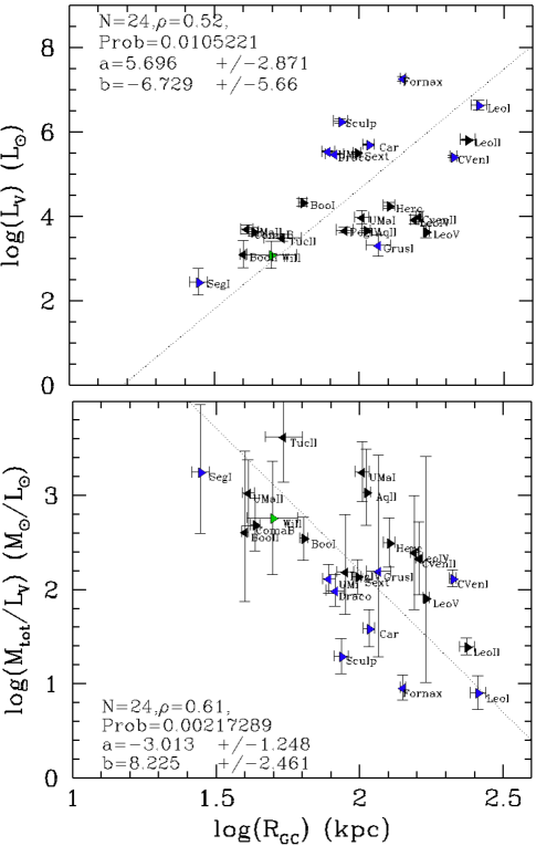
Figure 12: Correlation between $V$-band luminosity $L_{V}$ (top panel) and $M_{\rm tot}$/$L_{V}$ (bottom panel) with the galactocentric radius $R_{\rm GC}$.

The strong correlations found in Figures 7 and  9 are likely responsible for most correlations shown by dwarf galaxies all along this paper. Their impact is strong because they correspond to a theoretical prediction (see Eq. 13), for which MW dwarf galaxies are stellar systems out of equilibrium due to the severe impact caused by the gas removal and MW tidal shocks. However, one may wonder if there could be selection effects, e.g., due to the fact that not all the MW dwarfs have been discovered, or for which their velocity dispersion has not been determined, yet.

The top panel of Figure 12 reveals the trend between dwarf visible luminosity and galacto-centric distance. This could be due to selection effects as faint dwarfs are more difficult to be detected at larger distances (Drlica-Wagner et al., 2020). This may generate the anti-correlation between $M_{\rm tot}/L_{\rm V}$ and $R_{\rm GC}$, because $M_{\rm tot}$ has been calculated from Eq. 3, and does not correlate with $R_{\rm GC}$ (see red-dashed lines in Figure 8 for $X=1$).

One may wonder whether or not this possible selection effect can also be responsible of the correlations found in this paper. Figure 13 provides a negative answer, because the structural parameter that is the most correlated with the pericenter, $(\sigma_{\rm los}^{2}-\sigma_{\rm stars}^{2})$/$r_{\rm half}$, is not correlated with $L_{V}$. It results that the correlations between $(\sigma_{\rm los}^{2}-\sigma_{\rm stars}^{2})$/$r_{\rm half}$ and $R_{\rm peri}$ or $g_{\rm MW}$ are unlikely to be affected by selection effects.

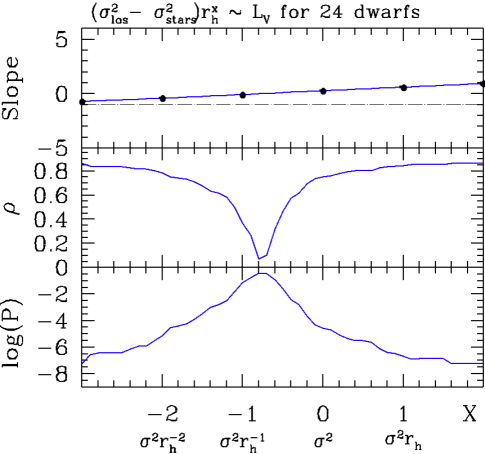
Figure 13: Slope, correlation $\rho$, and associated probability (in logarithmic scale) of the correlation between $\sigma_{\rm los}^{2}r_{\rm half}^{X}$ and $L_{V}$ from $X=-3$ to $X=2$. Each quantity is shown on the $X$ axis.

5.7 Are MW dwarf dark-matter contents over-estimated?

A recent arrival of most dwarfs in the MW halo, together with recent bursts of star formation, favors a scenario in which they have recently lost their gas, making them unstable against MW tides. The fact that most dwarfs are near their pericenter also supports the recent loss of gas together with MW tidal shocks. This is indicated by the correlations shown in Figures 7 and  9, which are theoretically predicted, as well as reproduced by simulations of Paper III.

However, we notice that the recent infall of MW dwarfs is justified by orbital arguments, with a timing scale coming from comparisons to former merger events in the MW halo (e.g., GSE and Sgr). This would have considerable consequences on the DM content of dwarf progenitors and then on that of MW dwarfs. As shown by Mayer et al. (2006), it would require several pericenter passages and a Hubble time to transform a DM-dominated rotating gas-rich dwarf into a gas-free, dispersion supported system. Here, this transformation needs to be done in just one orbit, which considerably limits the possible amount of DM. Paper III has simulated a DM-dominated progenitor of Sculptor, assuming the prescription from Eq. 3, which has been established by Wolf et al. (2010). It confirms that in the Sculptor orbital conditions, a rotating gas-rich dwarf cannot be transformed into a MW gas-free dwarf after one orbital time.

This scenario implies that most MW dwarfs as they are observed today are not in equilibrium. Their recent gas removal together with MW tidal shocks suffice to explain their high velocity dispersions, both from theory and simulations. It results that the self-equilibrium conditions assumed by Walker et al. (2009) and Wolf et al. (2010) cannot apply to MW dwarf galaxies, which questions the corresponding estimates of large mass excess when they are compared to the stellar mass. Consequently, this means that we have no way to prove or disprove the presence of dark matter in objects far from equilibrium.

6 Conclusions

Here, we have investigated how the structural (morphological and kinematical) properties of Milky Way globular clusters and dwarf spheroidals depend on their orbital properties. We have further limited our investigations to relations that do not depend on the adopted MW mass. We first confirm that the $r_{\rm half}\propto 1/E$ relation found in Paper I is robust to the adopted Milky Way mass model.

We also confirm that HSB-GCs are in pseudo-equilibrium with MW tidal shocks, removing approximately 3% of their mass at each pericenter passage. They differ from the more fragile LSB-GCs, which are strongly destabilized by MW tides, a significant fraction of them (27 %) possess tidal tails, and/or are in a tidal dominant regime (24%, see Figure 5).

Dwarf galaxies show some similarities with LSB-GCs. However, correlations between their structural and orbital properties are unexpected if they arrived recently into the MW halo and have no time to perform more than one orbit (see Paper I). Specifically the anti-correlation shown in Figure 7 or that found by Kaplinghat et al. (2019, see their Fig. 1) is in tension with MW dwarfs modeled as systems at self-equilibrium with large amounts of dark matter. Indeed, it is difficult to explain why new-coming sub-halos have their densities depending on pericenter without having time to be affected by MW tides (Cardona-Barrero et al., 2023).

A late infall for dwarfs requires one to consider the properties of their pre-infall progenitors outside the MW halo. They are likely gas-rich dwarf galaxies (Grcevich & Putman, 2009), and their passage into the MW halo gas may have fully transformed them into gas-free dwarf galaxies (Mayer et al., 2006; Yang et al., 2014). It suggests that most dwarf properties result from a temporal sequence, beginning with gas stripping due to MW halo gas ram-pressure, expansion of their stars due to the subsequent lack of gravity, and then a significant impact of MW tidal shocks exerted mostly on the leaving stars. The impact of such an out-of-equilibrium process has been theoretically described, and will be shown in Paper III simulations, for which a first example is provided in Figure 11. It is also consistent with the dwarf proximity to their pericenters, a property that otherwise would appear in contradiction with conservation of energy.

This scenario allows us to make the following predictions: Most MW dwarf galaxies (1) have velocity dispersion values with a significant contribution due to ram-pressure stripping and Galactic tidal shocks; (2) show many stars in their outskirts, their distances from the dwarf core depending on the elapsed time since the gas has been decoupled from stars; (3) show a small fraction of young stars, both in their cores and outskirts.

Condition (1) is fulfilled through Eq. 13 and Figure 9, as well as from simulations. Verification of condition (2) is on-going through the recent and successful discoveries of stars in the very outskirts of dwarfs (Sestito et al., 2023; Waller et al., 2023; Chiti et al., 2023; Cantu et al., 2021; Yang et al., 2022a; Roederer et al., 2023). Paper IV reveals that condition (3) is also fulfilled on the basis of a novel investigation of their CMDs. This series of papers (Papers I to IV) may change our understanding of MW dwarf galaxies, passing from an equilibrium model allowing mass estimates, to an out-of-equilibrium model that prevents mass estimates other than that of the baryonic mass.

Further simulations could be useful to verify which amount of dark matter they may contain for allowing their transformation into gas-free, dispersion-supported dwarfs in a single orbit, while preserving the correlations shown in Figures 7 and  9.

Data Availability

All necessary data used in this paper are available in the Tables of the Appendix B and in Li et al. (2021).

Appendix A About the infall time of dwarf galaxies

Barmentloo & Cautun (2023) proposed a machine learning technique to calculate the infall time of most MW dwarfs. Figure 14 compares their results for 25 dwarfs. This Appendix examines the robustness of their analysis, and compares it to results from cosmological simulations (Rocha et al., 2012). We make the following points.

• Barmentloo & Cautun find an infall epoch for Sgr (and other associated dwarfs, see green points) that is later than that of VPOS dwarfs, while the Sgr system has a much smaller energy (see Figure 14). This contradicts their own claim, i.e., quoting them, "we expect that there is a strong correlation between satellite orbital energy and infall time."

• The infall time for most dwarfs would be similar to that of the GSE major merger event in the MW, while the orbital energy of the later event is five times smaller;

• The use of non-independent input features (e.g., distance, radial and total velocity versus total energy and angular momentum) to derive the infall time may lead to unreliable results, because some of them show a flat profile versus the infall time, i.e., which likely dilutes the predictions;

• According to their fig. 4, their technique can only retrieve input infall times smaller than 3-4 Gyr, i.e., only for dwarfs shown in the bottom-left part of Figure 14;

• Their choice of host galaxy halos in the EAGLE simulation appears not representative of the MW past history, i.e., the significant increase of both pericenter and apocenter from 9 to 1 Gyr ago (see their Fig. 1) requires considerable mass gains, while MW is known to have experienced its last major merger 9-10 Gyr ago, as shown from the analysis of the GSE event (Naidu et al., 2021);

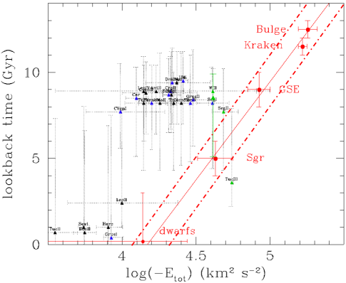
Figure 14: Comparison of the infall lookback time as a function of the orbital energy from Hammer et al. 2023, red dots and line joining MW merger events, which matches very well Rocha et al. 2012, the two red dot-dashed lines representing $\pm$$1\,\sigma$. Besides this analysis based on a strong correlation between satellite orbital energy and infall time, triangles represent individual dwarfs infall times based on the method of Barmentloo & Cautun (2023, see text), showing how these predictions are discrepant from the expected relation with total orbital energy. The dwarfs associated with the VPOS and with Sgr are shown in blue and green, respectively.

Additionally, the choice of Barmentloo & Cautun (2023) to define the infall time as being the first time the future satellite is passing through the virial radius of the host lead to very scattered results according to Rocha et al. (2012). Consequently, predictions for infall times are better predicted through their tight correlation with orbital energy (Rocha et al., 2012), the latter being calculated with good accuracy from Gaia DR3 (see Paper I).

We also noticed the study by Pagnini et al. (2022), which may cast some doubts about the reliability of associating GCs to past merger events in the MW (Kruijssen et al., 2019; Kruijssen et al., 2020; Malhan et al., 2022). However, this might be due to the following assumptions (1) that GCs originate in halos of infalling dwarfs and are not formed during merger events (e.g., Kraken GSE, or Pontus) that likely induced strong star formation events 12 to 9 Gyr ago (Haywood et al., 2016), (2) that all mergers experienced by the MW, including GSE, were minor (e.g., mass ratio of 1:10), contrary to the analysis by Naidu et al. (2021) who considered mass ratio from 1:2 to 1:4 and (3) that simulations without gas can reproduce the infall of stellar systems at epochs when the gas is preponderant. It is unlikely that all GCs have been formed through the way proposed by Pagnini et al. (2022). However, the latter study provides a complementary channel for explaining several GCs that are not identified inside a structure in the plane made by total energy and angular momentum (see Fig. 5 of Paper I).

Appendix B Intrinsic parameters of MW dwarf galaxies

Table LABEL:tab:struct describes the structural parameters of the MW dwarf galaxies. Column 1: dwarf galaxy name; Column 2: V- luminosity; Column 3: stellar mass to light ratio; Column 4: Galacto-centric distance; Column 5: half-light radius or effective radius; Column 6: dwarf ellipticity; Column 7: line of sight velocity dispersion; Column 8: velocity dispersion due to the sole stellar component.

Data of Table LABEL:tab:struct are taken from the review by Simon (2019, see also references therein), and have been updated by more recent measurements. The latter include:

• New estimates of $\sigma_{\rm los}$ for Bootes I, Leo IV, and LeoV (Jenkins et al., 2021);

• Last update by Josh Simon of Simon (2019) with a new value for $\sigma_{\rm los}$ of Grus I, and Leo V;

• New measurements from Bruce et al. (2023) of $\sigma_{\rm los}$ for Aquarius II (8 spectroscopic stars, 4.7 instead of 5.4) and Bootes II (2.9 instead of 8.2!);

• First robust measurements of $\sigma_{\rm los}$ of Pegasus IV (Cerny et al., 2023);

• Data for both Antlia II and Crater II (Caldwell et al., 2017; Torrealba et al., 2016; Torrealba et al., 2019; Ji et al., 2021).

The sample of dwarf galaxies comes from table 1 of Li et al. (2021) for 46 dwarfs. Here, we only include objects within 300 kpc (excluding Eridanus II), and for which a measurement of $\sigma_{\rm los}$ has been performed without ambiguity. The latter condition leads to remove 5 dwarf galaxies having less than 5 stars with both Gaia and spectroscopy data. It would lead to 40 dwarfs, to which we have further removed the 3 potential GCs (Crater, Draco II, and Sgr II), and 5 dwarfs (Carina II, Carina III, Phoenix II, Horologium I, Hydrus I, and Reticulum II) associated to the LMC. Also associated to the LMC, Carina III is already excluded since only 4 of its stars possess spectroscopy. Similarly, Columba I (3), Horologium II (1), Pisces II (3), and Reticulum III (3) are not considered due to their lack of spectroscopic stars (which numbers are given in parenthesis). Finally, we have also removed Grus II, Hydra II, Segue 2, Triangulum II, Tucana III, Tucana IV, and Tucana V, because only a limit on their velocity dispersion can be determined (Simon, 2019, see also references therein).

However, in this paper, we have reintegrated Aquarius II (8 spectroscopic stars) and Pegasus IV, since for both galaxies their velocity dispersion has been measured. It leaves us with a sample of 26 galaxies, all with more than 10 spectroscopic stars, except for Aquarius II, Grus I, Leo IV, Leo V, Pegasus IV, Ursa Major II, and willman.

Table 2: Structural properties of Milky Way dwarfs including kinematics.

name	$L_{\rm V}$	$M_{\rm stars}/L_{\rm V}$	$R_{\rm GC}$	$r_{\rm half}$	$\epsilon$	$\sigma_{\rm los}$	$\sigma_{\rm stars}$
	$(L_{\rm sun}$)		(kpc)	(pc)		(km s-1)	(km s-1)
Antlia II	$214,783\pm 29,600$	$2.5$	$130.35^{+6.5}_{-6.5}$	$2867^{+312}_{-312}$	$0.38$	$5.71^{+1.08}_{-1.08}$	$0.317\pm 0.039$
Aquarius II	$4742\pm 613.2$	$2.5$	$105.40^{+3.3}_{-3.3}$	$160^{+26}_{-26}$	$0.39$	$4.7^{+1.8}_{-1.2}$	$0.2\pm 0.029$
Bootes I	$21,880\pm 5082$	$2.5$	$63.64^{+2}_{-2}$	$191^{+8}_{-8}$	$0.30$	$5.1^{+0.6}_{-0.7}$	$0.392\pm 0.054$
Bootes II	$1282\pm 955$	$2.5$	$39.82^{+1}_{-1}$	$39^{+5}_{-5}$	$0.25$	$2.9^{+1.6}_{-1.2}$	$0.210\pm 0.092$
CanesVenatici I	$265,500\pm 14,680$	$2.5$	$210.8^{+6}_{-6}$	$437^{+18}_{-18}$	$0.44$	$7.6^{+0.4}_{-0.4}$	$0.90\pm 0.043$
CanesVenatici II	$10,000\pm 2990$	$2.5$	$160.6^{+4}_{-4}$	$71^{+11}_{-11}$	$0.40$	$4.6^{+1}_{-1}$	$0.435\pm 0.098$
Carina	$515,200\pm 23,740$	$2.5$	$107.6^{+5}_{-5}$	$311^{+15}_{-15}$	$0.36$	$6.6^{+1.2}_{-1.2}$	$1.49\pm 0.070$
ComaBerenices	$4406\pm 1023$	$2.5$	$43.19^{+1.55}_{-1.55}$	$69^{+4.5}_{-4.5}$	$0.37$	$4.6^{+0.8}_{-0.8}$	$0.29\pm 0.0435$
Crater II	$162,900\pm 15,030$	$2.5$	$116.4^{+1.1}_{-1.1}$	$1066^{+86}_{-86}$	$0$	$2.7^{+0.3}_{-0.3}$	$0.453\pm 0.039$
Draco	$304,800\pm 14,040$	$2.5$	$81.98^{+6}_{-6}$	$231^{+17}_{-17}$	$0.29$	$9.1^{+1.2}_{-1.2}$	$1.331\pm 0.079$
Fornax	$18,540,000\pm 2,397,000$	$1.5$	$141^{+3}_{-3}$	$792^{+18}_{-18}$	$0.29$	$11.7^{+0.9}_{-0.9}$	$4.34\pm 0.330$
Grus I	$3732\pm 1192$	$2.5$	$116.2^{+11.5}_{-11.5}$	$28^{+23}_{-23}$	$0.44$	$2.9^{+2.1}_{-1}$	$0.423\pm 0.241$
Hercules	$18,370\pm 28867$	$2.5$	$126.4^{+6}_{-6}$	$216^{+20}_{-20}$	$0.69$	$5.1^{+0.9}_{-0.9}$	$0.338\pm 0.042$
Leo I	$4,406,000\pm 1,149,000$	$1.5$	$257.8^{+15.5}_{-15.5}$	$270^{+16.5}_{-16.5}$	$0.30$	$9.2^{+0.4}_{-0.4}$	$3.62\pm 0.58$
Leo II	$673,000\pm 24,800$	$2.5$	$235.5^{+14}_{-14}$	$171^{+10}_{-10}$	$0.07$	$7.4^{+0.4}_{-0.4}$	$2.3\pm 0.10$
Leo IV	$8472^{\pm}2048$	$2.5$	$154.6^{+5}_{-5}$	$114^{+13}_{-13}$	$0.17$	$3.3^{+1.7}_{-1.7}$	$0.316\pm 0.056$
Leo V	$4446\pm 1501$	$2.5$	$169.8^{+4}_{-4}$	$49^{+16}_{-16}$	$0.43$	$2.3^{+3.2}_{-1.6}$	$0.349\pm 0.115$
Pegasus IV	$4800\pm 800$	$2.5$	$89^{+6}_{-6}$	$41^{+8}_{-8}$	$0.20$	$3.3^{+1.7}_{-1.1}$	$0.396\pm 0.071$
Sculptor	$1,820,000\pm 235,300$	$2.5$	$86.09^{+5}_{-5}$	$279^{+16}_{-16}$	$0.33$	$9.2^{+1.1}_{-1.1}$	$2.96\pm 0.27$
Segue 1	$283\pm 205$	$2.5$	$27.84^{+2}_{-2}$	$24^{+4}_{-4}$	$0.33$	$3.7^{+1.4}_{-1.1}$	$0.1259\pm 0.056$
Sextans	$322,100\pm 17,810$	$2.5$	$97.97^{+3}_{-3}$	$456^{+15}_{-15}$	$0.30$	$7.9^{+1.3}_{-1.3}$	$0.97\pm 0.042$
Tucana II	$3105\pm 575$	$2.5$	$54.24^{+8}_{-8}$	$121^{+35}_{-35}$	$0.39$	$8.6^{+4.4}_{-2.7}$	$0.185\pm 0.044$
UrsaMajor I	$9638\pm 3443$	$2.5$	$101.9^{+5.85}_{-5.85}$	$295^{+28}_{-28}$	$0.59$	$7^{+1}_{-1}$	$0.2095\pm 0.047$
UrsaMajor II	$5058\pm 1223$	$2.5$	$40.81^{+1.95}_{-1.95}$	$139^{+9}_{-9}$	$0.56$	$5.6^{+1.4}_{-1.4}$	$0.221\pm 0.033$
UrsaMinor	$349,900^{\pm}16,120$	$2.5$	$77.89^{+4}_{-4}$	$405^{+21}_{-21}$	$0.55$	$9.5^{+1.2}_{-1.2}$	$1.0776\pm 0.0527$
Willman 1	$1236\pm 909$	$2.5$	$49.62^{+10}_{-10}$	$33^{+8}_{-8}$	$0.47$	$4^{+0.8}_{-0.8}$	$0.224\pm 0.109$

Dwarf	EinastoHM	NFW	EinastoMM	EinastoLM
AntliaII	0.454	0.414	0.494	1.08
AquariusII	0.312	0.581	1.31	3.001
BootesI	0.333	0.444	0.649	1.55
BootesII	0.641	0.91	1.803	2.968
CanesVenaticiI	0.599	0.659	0.829	1.301
CanesVenaticiII	0.728	0.765	0.875	0.998
Carina	0.076	0.303	0.871	2.347
ComaBerenices	0.323	0.471	0.656	1.549
CraterII	0.603	0.584	0.598	0.764
Draco	0.413	0.456	0.573	1.217
Fornax	0.361	0.262	0.325	1.099
GrusI	0.821	0.913	1.446	1.795
GrusII	0.478	0.538	0.594	0.884
Hercules	0.608	0.763	1.231	2.196
HydraII	1.874	3.614	5.912	11.23
LeoI	0.9	1.539	1.885	3.056
LeoII	0.512	0.474	0.607	0.954
LeoIV	0.594	0.745	0.899	1.268
LeoV	0.967	2.438	4.469	8.846
PegasusIV	0.52	0.476	0.448	0.455
Sculptor	0.323	0.365	0.518	1.308
Segue1	0.475	0.525	0.572	0.821
Segue2	0.416	0.404	0.398	0.399
Sextans	0.385	0.752	1.614	3.375
TriangulumII	0.802	0.861	0.935	1.732
TucanaII	0.682	0.955	1.872	2.982
TucanaIII	0.873	0.881	0.886	0.91
TucanaIV	0.357	0.429	0.521	1.07
TucanaV	0.609	0.765	1.336	2.278
UrsaMajorI	0.318	0.247	0.272	0.565
UrsaMajorII	0.476	0.649	0.927	2.056
UrsaMinor	0.372	0.372	0.43	0.857
Willman	0.249	0.247	0.265	0.332

Appendix C Properties of pericenter velocity

Figure LABEL:fig:Vper_Rper shows that for GCs, $V_{\rm peri}$ is rather constant (logarithmic slope $-0.16$) with large variations of $R_{\rm peri}$:

$$V_{\rm peri}=V_{\rm peri}=398\,\rm km\,s^{-1}\,R_{\rm peri}^{-0.16}$$ (14)

The slope is slightly steeper for dwarfs (-0.2), which also show a stronger correlation ($\rho$= 0.9) than GCs.

References

- Aguilar & White (1985) Aguilar L. A., White S. D. M., 1985, ApJ, 295, 374
- Aguilar et al. (1988) Aguilar L., Hut P., Ostriker J. P., 1988, ApJ, 335, 720