Probabilistic Inference of the Structure and Orbit of Milky Way Satellites with Semi-Analytic Modeling

Abstract

Semi-analytic modeling furnishes an efficient avenue for characterizing the properties of dark matter halos associated with satellites of Milky Way-like systems. Unlike previous approaches, this method easily accounts for uncertainties arising from halo-to-halo variance, the orbital disruption of satellites, baryonic feedback, and the stellar-to-halo mass (SMHM) relation. We use the SatGen semi-analytic satellite generator—which incorporates both empirical models of the galaxy–halo connection in the field as well as analytic prescriptions for the orbital evolution of these satellites after they enter a host galaxy—to create large samples of Milky Way-like systems and their satellites. By selecting satellites in the sample that match the observed properties of a particular dwarf galaxy, we can then infer arbitrary properties of the satellite galaxy within the Cold Dark Matter paradigm. For the Milky Way’s classical dwarfs, we provide inferred values (with associated uncertainties) for the maximum circular velocity $v_{\text{max}}$ and the radius $r_{\text{max}}$ at which it occurs, varying over two choices of feedback model and two prescriptions for the SMHM relation that populate dark matter halos with physically distinct galaxies. While simple empirical scaling relations can recover the median inferred value for $v_{\text{max}}{}$ and $r_{\text{max}}{}$, this approach provides more realistic correlated uncertainties and aids interpretability by allowing for the feedback model to vary. For these different models, we also demonstrate how the internal properties of a satellite’s dark matter profile correlate with its orbit, and we show that it is difficult to reproduce observations of the Fornax dwarf without strong baryonic feedback. The technique developed in this work is flexible in its application of observational data and can leverage arbitrary information about the satellite galaxies to make inferences about their dark matter halos and population statistics. The code and datasets are available at https://github.com/folsomde/Semianalytic_Inference for use in extensions of this analysis or as input for other studies.

1 Introduction

The satellite galaxies of the Milky Way (MW) have long been of interest as probes of cosmological structure formation and of the influence of dark matter (DM) at small scales. The most luminous of the MW’s satellites, the “classical” satellites, are especially promising candidates for such studies. These dwarf galaxies have stellar populations large enough to provide robust measurements of galactic properties while still maintaining a low stellar-to-halo mass ratio, making them ideal for DM studies. This work proposes a novel semi-analytic formalism that enables the prediction of many properties (with associated uncertainty) for dwarf galaxies undergoing disruption in a MW-like host system, given their present-day observable properties. Using this procedure, we (i) infer the halo structure for each of the MW’s classical satellites and compare it to existing analyses, (ii) provide a novel means by which models of baryonic feedback may be constrained, and (iii) demonstrate the connection between internal properties of the satellites and their orbital properties, including a study of whether or not the satellites were accreted from the field or as part of a larger system.

There is a long tradition of study surrounding the “galaxy–halo connection,” which establishes broad-strokes statistical relationships between luminous galaxies and their DM halos—see Wechsler & Tinker (2018) for a review. In the Cold Dark Matter (CDM) paradigm, DM halos provide the gravitational wells that capture baryonic gas and seed galaxy growth. The naive expectation, which has been borne out by detailed empirical and analytical studies (Conroy et al., 2006; Behroozi et al., 2013; Moster et al., 2013), is that there is a direct relationship between galaxy and halo size, with more massive halos containing more massive galaxies. This relationship, the stellar mass–halo mass (SMHM) relation, is a core ingredient in semi-analytic models and has a modest scatter, at least for systems with peak halo masses above $\sim 10^{11}~{}M_{\odot}$. Below this scale, uncertainties on both the slope and scatter of the SMHM distribution can be significant—see, e.g., Danieli et al. (2023) and references therein—and predictions for dwarf systems can vary drastically (Behroozi et al., 2010; Behroozi et al., 2019; Nadler et al., 2019). This uncertain region of parameter space includes many MW satellites, and as such they provide an interesting laboratory for understanding this aspect of the galaxy–halo connection.

The galaxy–halo connection grows in complexity beyond the SMHM relation. Baryons gravitationally influence the DM halos in which they reside, and there is a wealth of literature surrounding how these “baryonic feedback” mechanisms affect the structure of the DM halo and the uncertainties inherent in modeling this feedback (see, e.g., Vogelsberger et al., 2020). The structure of an isolated halo can be described through empirical relations between, e.g., the halo mass and a concentration parameter or the maximum circular velocity (Neto et al., 2007; Moliné et al., 2017). However, these relations become further complicated for satellite galaxies that undergo complex tidal interactions with their hosts (Peñarrubia et al., 2009). These interactions can lead to deviations from predictions for isolated halos and potentially even to total disruption of the satellite. The tidal evolution depends on the structure of the satellite halo, which in turn depends on its baryonic content. The current state-of-the-art for modeling these intricate systems is through (magneto)hydrodynamical simulations, which must assume particular models for star formation, baryonic feedback, etc., and which require significant computational resources to resolve large numbers of dwarf galaxies. Moreover, such simulations are prone to numerical artifacts, such as artificial disruption (van den Bosch et al., 2018; van den Bosch & Ogiya, 2018), which affect characterizations of their satellite populations.

This paper proposes a new strategy for inferring the halo properties of satellite galaxies. The procedure relies on semi-analytic satellite generators to address several of the challenges listed above. Such generators combine empirical modeling of the galaxy–halo connection as parameterized from simulations, along with analytic modeling of tidal mass loss and dynamical friction, to find the orbital path and mass evolution of a satellite galaxy. The semi-analytic code can efficiently generate satellite populations for individual MW halos and then incorporate halo-to-halo variance by generating many such iterations. There are three key advantages of this approach. First, the large statistical samples that can be generated allow one to find a population of satellites that closely resemble any satellite of interest based on observational data. Second, the comparatively low computational cost allows one to efficiently scan over known sources of uncertainty, especially with regards to parameterizations of the SMHM relation and feedback mechanisms, providing a means to effectively quantify systematic uncertainties on the predictions. Finally, the realizations of the semi-analytic model each carry detailed information about many internal and systemic properties of their satellites that can be leveraged in analyses.

Semi-analytic models have long been employed for the study of dwarf galaxy formation, particularly in recovering the population of MW satellites as a whole. In practice, much of this literature centers around matching population statistics such as the luminosity function or mass function of the MW satellite system (Koposov et al., 2009; Li et al., 2010; Macciò et al., 2010; Guo et al., 2011; Font et al., 2011; Brooks et al., 2013; Starkenburg et al., 2013; Barber et al., 2014; Pullen et al., 2014; Guo et al., 2015; Lu et al., 2016; Nadler et al., 2019, 2023). As an extension of this body of work, semi-analytic models can also be applied to the evolution of individual satellites as part of such a system (Taylor & Babul, 2001; Peñarrubia et al., 2010; Hiroshima et al., 2018; Ando et al., 2020; Dekker et al., 2022).

In this vein, the current study uses the semi-analytic model SatGen, which provides a statistical sample of MW-like satellite systems with adjustable parameters for the initialization and evolution of satellite galaxies, as discussed below. SatGen is able to accurately reproduce distributions of satellite maximal circular velocity, $v_{\text{max}}$, the radius at which this velocity occurs, $r_{\text{max}}$, and the spatial distributions of observed satellite populations of the MW and M31 (Jiang et al., 2021), as well as those produced by cosmological zoom-in simulations (Sawala et al., 2016; Garrison-Kimmel et al., 2017). These distributions are produced by integrating the orbits of satellite subhalos, tracking the evolution of their density profiles and the galaxies they may host. As it does not require merger trees from an extant simulation, SatGen can efficiently sample cosmologically-motivated assembly histories, which enables it to capture the dramatic halo-to-halo variance of satellite statistics. Further, SatGen is calibrated to reproduce baryonic feedback seen in hydrodynamical simulations and self-consistently tracks tidal mass loss and the resultant density profile evolution during a satellite’s orbit, as described in detail in Section 2.1 and the references therein.

To model the halo of a particular satellite galaxy, we select satellite analogues from the overall SatGen distribution in a principled way based on their similarity to the galaxy we wish to model. The result of this selection is impacted by both the choice of the galaxy–halo connection model and by the selection criteria, i.e., the incorporation of different sets of observables into the selection. The analysis finds good agreement with existing studies of the MW’s classical satellites, recovering reasonable parameter values with physically-motivated uncertainties.

The results of this work have broad applicability to the study of MW substructure. For any property of interest of a MW satellite, the method introduced here allows for inference of the allowed range of values consistent with arbitrary prior information. Throughout the text, we illustrate this advantage by giving examples of inference for both internal properties of the DM halos of various MW satellite galaxies as well as distributions for orbital properties of these objects. The method presented in this paper can be used to constrain models of baryonic feedback, to probe the galaxy–halo connection, and to understand the spread of parameter values consistent with the observed properties of any individual satellite galaxy. In particular:

• Using our proposed technique on the Fornax dwarf galaxy provides interesting results. Specifically, we find that observations of the central density and stellar mass of Fornax are difficult to reproduce under assumptions of minimal baryonic feedback. A model including stronger DM core formation is required to produce both parameters simultaneously.

• We have compared our new method to similar inference methods based on the use of simple scaling relations, such as abundance matching. We find that while these techniques are able to recover reasonable estimates for the structural parameters of the MW’s classical satellites, the inferred uncertainties do not properly reflect the complexities of nonlinear satellite evolution and are typically underestimated.

• Using the techniques presented in this paper, we infer that it is unlikely that any of the classical satellites of the MW was part of a larger system at the time of accretion into the Galaxy, though the mode of accretion (i.e., whether directly accreted from the field or accreted as part of a group) significantly affects aspects of the orbit.

The paper is organized as follows. Section 2 overviews the methodology, reviewing SatGen and discussing the statistical procedures used in the study. As a concrete example, Section 3 applies this method to infer profile parameters for the MW’s classical satellites — specifically the radius $r_{\text{max}}{}$ at which the maximum circular velocity, $v_{\text{max}}{}$, is achieved. Also included is a discussion of the systematic uncertainties associated with this modeling, demonstrating that the resulting predictions in the $r_{\text{max}}$ – $v_{\text{max}}$ plane correspond well to observational studies. Section 4 provides other applications of the method by (i) correlating internal structure with orbital properties by considering the relation between pericentric distance and central density and (ii) discussing the likelihood that the classical satellites of the MW were contributed by the infall of a large system of satellites. Section 5 summarizes the main findings of this study.

2 Methodology

The method presented in this paper requires a large sample of realistic MW satellites. This statistical sample is generated using a semi-analytic model of halo formation, described in Section 2.1, that efficiently produces a population of satellites not subject to artificial disruption. Moreover, the model enables variation of the systematic uncertainties that contribute to structure formation, including baryonic feedback, the SMHM relation, and halo-to-halo variance. This diverse, physically-motivated sample of satellite systems provides the backbone for a weighting procedure that can be used to make predictions for particular dwarf galaxies of interest. The weighting procedure is described in Section 2.2.

2.1 Semi-Analytic Satellite Generation

2.1.1 SatGen Overview

In this work, we use the SatGen semi-analytic halo model (Jiang et al., 2021; Green et al., 2022) and refer the reader to the original publications for more details on the implementation of the model and its calibration. The model generates satellite populations in two steps. First, it generates hierarchical merger trees according to the extended Press–Schechter theory (Parkinson et al., 2007) and initializes the progenitor halos for a target host of a particular mass (in this case, the target is a MW-like halo). Second, it evolves the orbit and internal structure of each progenitor halo according to physical prescriptions and empirical relations calibrated to high-resolution simulations. Ultimately, this produces a realistic population of surviving satellites around the target host.

Satellite progenitors at infall are assigned with cosmologically-motivated initial orbits (Li et al., 2020), density profiles (Zhao et al., 2009; Freundlich et al., 2020), and stellar masses. The functional form for the halo profiles, introduced by Dekel et al. (2017), belongs to the $\alpha\beta\gamma$ family of profiles (Zhao, 1996). Freundlich et al. (2020) have shown that its four free parameters have the flexibility required to describe the DM halo’s response to baryonic processes. A convenient parameterization of this profile uses the virial mass of the halo, a concentration parameter, the slope of the density profile at $1\%$ of the virial radius, and the spherical virial overdensity.

The merger tree sets the virial mass and time of infall (which in turn determines the virial overdensity) for each accreted object, and SatGen determines the two remaining parameters as follows. The concentration parameter is first calculated following the universal model of Zhao et al. (2009), which is based on cosmological DM-only simulations with a wide range of cosmological parameters. Then, the stellar mass is determined using a SMHM relation, detailed below. The halo parameters are set such that they respond appropriately to baryonic effects: the inner slope of the density profile and the updated concentration parameter are calculated according to empirically-calibrated relations from hydrodynamical simulations (e.g., Tollet et al., 2016; Freundlich et al., 2020). This procedure fully determines the initial conditions of the galaxy and its DM halo. The merger tree algorithm then recurses, describing the assembly history of each satellite before falling into the MW.

SatGen accounts for scatter in each of the aforementioned scaling relations. Notably, the SMHM relation is given a scatter of 0.2 dex in stellar mass, and the feedback prescriptions include additional scatter on the concentration parameter. An advantage of using a semi-analytic model is that one can sample effectively over this scatter, allowing for full exploration of reasonable satellite parameter space.

After initializing the DM and stellar properties of the satellites at infall, SatGen evolves their orbit and structure within the dynamically evolving host potential, including a Chandrasekhar (1943)-like treatment of dynamical friction. Internally, the satellites evolve along tidal tracks, which are empirical laws for the structural response of the satellites to tidal stripping and heating (Peñarrubia et al., 2010; Errani et al., 2018; Green & van den Bosch, 2019). The combined effect of these prescriptions is another important advantage of this semi-analytic orbit integration approach: the evolution of a satellite’s internal structure is self-consistently accounted for with a formalism that is computationally cheap when compared to full numerical simulations. However, the formalism does lack some notable dynamical effects. Specifically, while SatGen accounts for hierarchical structure formation, allowing for satellites to host (and potentially eject) their own satellites, it does not account for tidal effects beyond those of the immediate parent, nor does it account for gravitational interactions between satellites of the same order, or for the back-reaction of the satellites on the host potential.

2.1.2 Stellar Mass–Halo Mass Relation

An important source of systematic uncertainty is the SMHM relation. SatGen provides two possible calibrations for this relation, based on either the Rodríguez-Puebla et al. (2017, hereafter RP17) model or the Behroozi et al. (2013, hereafter B13) model. Both parameterize the stellar-to-halo mass ratio, $X=M_{\star}/M_{\mathrm{vir}}$, in terms of $M_{\mathrm{vir}}$. On the $M_{\star}$ – $M_{\mathrm{vir}}$ plane, the SMHM relations are effectively power laws (with some scatter) at the low-mass end, $M_{\mathrm{vir}}\lesssim 10^{10.5}~{}M_{\odot}$ (Behroozi et al., 2010; Munshi et al., 2021). The index of this power law at the low-mass end (often denoted $\alpha$) contains information regarding the star-formation efficiency and stellar feedback in dwarf halos. The default behavior in SatGen is to use the model presented in RP17, which has a fairly steep faint-end slope, $M_{\star}\propto M_{\mathrm{vir}}^{1.975}$ consistent with other recent studies—see, e.g., Behroozi et al. (2019) and references therein. However, this relation is very uncertain in the mass range of the classical satellites: B13 fit a much shallower slope of $M_{\star}\propto M_{\mathrm{vir}}^{1.412}$ in this regime. With a shallower slope, galaxies of the same stellar mass can reside in much lighter halos, which can significantly change the physics of galaxy evolution.

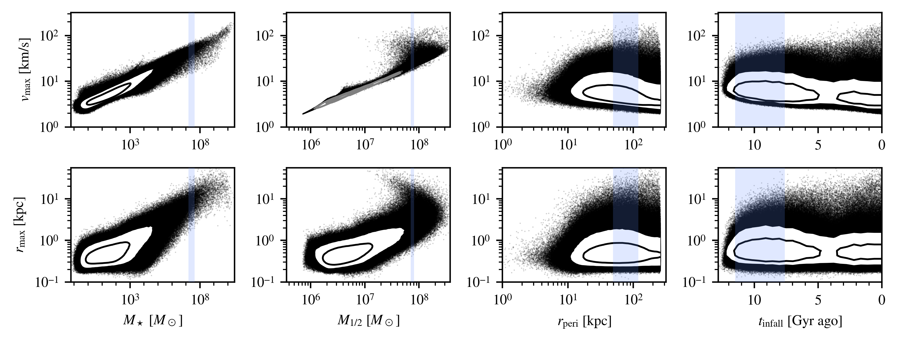
Figure 1: The satellites of all SatGen realizations form a correlated probability distribution in a high-dimensional space, shown with contours enclosing 68% and 95% of satellites, while those outside the contours are shown as individual points. This figure shows the joint distribution of profile parameters $(r_{\text{max}},\,v_{\text{max}})$ against (i) the stellar mass $M_{\star}$, (ii) the mass $M_{1/2}$ contained within Fornax’s half-light radius, (iii) the pericenter $r_{\mathrm{peri}}$, and (iv) the infall time $t_{\mathrm{infall}}$. Because many of these parameters correlate with $r_{\text{max}}$ and $v_{\text{max}}$, they can be used to infer these halo properties. As an example, the blue bands highlight the 68% confidence regions for the Fornax dwarf, collected in Table 1. SatGen satellites that lie in these bands contribute most strongly to the inference of Fornax’s halo profile parameters, following the procedure detailed in Section 2.2. These satellites are generated with the SMHM relation of RP17 and use the NIHAO-calibrated feedback emulator. The strong core formation of this model can be seen in the second column, where the large ratio of stellar mass to halo mass puffs up the satellites, leading to a population with large values for $r_{\text{max}}$ and $v_{\text{max}}$ with a relatively small $M_{1/2}$. The turnover in these panels is not present in the APOSTLE feedback emulator. Note that the sub-unity values in the $M_{\star}$ space reflect extrapolations of the semi-analytic tidal tracks of Errani et al. (2018), which allow for tidal stripping to be tracked even below what is physically meaningful. The region of interest is well within the reasonable parts of this space, but the full distribution is shown for clarity.

2.1.3 Baryonic Feedback

An additional source of systematic uncertainty is the baryonic feedback prescription, and SatGen provides two possible calibrations for this relation as well. The strength of the baryonic feedback can have a significant effect on dwarf halo profiles, particularly in the inner regions of halos that host large galaxies. In SatGen, the feedback model is parameterized by $X=M_{\star}/M_{\mathrm{vir}}$ and affects (i) the logarithmic slope $s_{0.01}$ of the profile at $1\%$ of the virial radius $r_{\mathrm{vir}}$, as well as (ii) the concentration, defined as $c_{-2}=r_{\mathrm{vir}}/r_{-2}$, where $r_{-2}$ is the radius at which the density profile is instantaneously a power law with index $-2$. The two prescriptions for baryonic feedback provided in SatGen reflect results from either the APOSTLE (Sawala et al., 2016) or NIHAO (Wang et al., 2015) simulations. The former exhibits much milder feedback, with the primary effect of the baryonic component on classical-mass satellites being the adiabatic contraction of the DM halo (Gnedin et al., 2004). NIHAO, on the other hand, has stronger baryonic feedback and allows for the formation of cores in the DM halos. Since these feedback relations depend on $X$, the strength of the feedback is sensitive to the choice of the SMHM relation.

2.1.4 Statistical Sample

The SatGen sample used in this work consists of a primary dataset of 4,000 MW realizations produced with the NIHAO feedback emulator and RP17 model, as well as 2,000 MW realizations for the three other combinations of feedback prescriptions and the SMHM models to which it is compared. This gives a total of 10,000 satellite systems. The size of the dataset ensures a thorough sampling of halo-to-halo variance in the assembly history. This is important for any study of classical satellites, as large satellites are somewhat rare; they sample the tail of the subhalo mass function. From the SatGen output, we consider first-order satellites of the MW (i.e., ignoring satellites of satellites) that are within the MW’s virial radius and that are gravitationally bound to the MW. We make two additional quality cuts. First, we remove satellites that have lost more than 99% of their virial mass to avoid satellites stripped beyond the range of calibration for the Errani et al. (2018) tidal tracks. This selection cut is physically motivated since it is unlikely that the satellites considered in this study have had such significant mass loss (Battaglia et al., 2022). Second, we remove satellites that have an ill-defined profile parameter $\alpha\geq 3$ (the $\alpha$ parameter is defined in terms of the concentration $c_{-2}$ and the slope $s_{0.01}$ described above, not to be confused with the notation used for the SMHM relation). If the profile is particularly cuspy or centrally concentrated, the definition can require $\alpha\geq 3$, which leads to unphysical negative densities (Freundlich et al., 2020). The current implementation of SatGen does not prevent this from happening, necessitating manual intervention. As a final cut, the mass resolution of the model is set to $10^{6.5}~{}M_{\odot}$; as soon as a satellite is stripped enough to fall below this limit, its orbit is no longer tracked. Depending on the choice of feedback model, the SMHM relation, and dwarf of interest, there are typically hundreds to thousands of classical satellite analogues in the sample—see Table 2 for a summary.

Name	$\log_{10}M_{\star}\,/\,M_{\odot}$	$\log_{10}M_{1/2}\,/\,M_{\odot}$	$r_{1/2}$ [pc]	$r_{\mathrm{peri}}$ [kpc]	$t_{\mathrm{infall}}$ [Gyr]	$D_{\mathrm{MW}}$ [kpc]
Canes Venatici I	$5.53_{-0.18}^{+0.18}$	$7.26_{-0.05}^{+0.05}$	$453.7_{-18.0}^{+18.0}$	$84.5_{-37.2}^{+53.6}$	$9.4_{-2.3}^{+0.9}$	217.8
Carina	$5.78_{-0.18}^{+0.18}$	$7.00_{-0.16}^{+0.16}$	$331.8_{-18.8}^{+18.8}$	$77.9_{-17.9}^{+24.1}$	$9.9_{-2.7}^{+0.6}$	106.7
Draco	$5.50_{-0.18}^{+0.18}$	$7.15_{-0.03}^{+0.03}$	$251.2_{-8.7}^{+8.7}$	$58.0_{-9.5}^{+11.4}$	$10.4_{-3.1}^{+2.4}$	76.0
Fornax	$7.40_{-0.22}^{+0.22}$	$7.88_{-0.03}^{+0.03}$	$836.3_{-17.1}^{+17.1}$	$76.7_{-27.9}^{+43.1}$	$10.7_{-3.1}^{+0.8}$	149.1
Leo I	$6.72_{-0.27}^{+0.27}$	$7.26_{-0.04}^{+0.04}$	$306.1_{-14.5}^{+14.5}$	$47.5_{-24.0}^{+30.9}$	$2.3_{-0.5}^{+0.6}$	256.0
Leo II	$5.91_{-0.18}^{+0.18}$	$6.88_{-0.05}^{+0.05}$	$199.5_{-10.6}^{+10.6}$	$61.4_{-34.7}^{+62.3}$	$7.8_{-2.0}^{+3.3}$	235.7
Sextans	$5.59_{-0.20}^{+0.20}$	$7.47_{-0.04}^{+0.04}$	$600.8_{-21.1}^{+23.4}$	$82.2_{-4.3}^{+3.8}$	$8.4_{-0.9}^{+2.7}$	89.2
Sculptor	$6.34_{-0.22}^{+0.22}$	$7.36_{-0.03}^{+0.03}$	$323.8_{-8.0}^{+8.0}$	$44.9_{-3.9}^{+4.3}$	$9.9_{-2.9}^{+1.7}$	86.1
Ursa Minor	$5.62_{-0.18}^{+0.18}$	$7.21_{-0.04}^{+0.04}$	$360.9_{-20.4}^{+20.4}$	$55.7_{-7.0}^{+8.4}$	$10.7_{-2.0}^{+1.7}$	78.0

Table 1: The observational values for the stellar mass $M_{*}$, half-light mass $M_{1/2}$, 3D circularized half-light radius $r_{1/2}$, pericentric distance $r_{\mathrm{peri}}$, the infall time $t_{\mathrm{infall}}$, and the galactocentric distance $D_{\mathrm{MW}}$ used for the nine bright MW spheroidal dwarf satellites in this work. Stellar masses are derived from Muñoz et al. (2018), using a mass-to-light ratio of 1.2 $M_{\odot}/L_{\odot}$ with an added uncertainty of 0.16 dex (Woo et al., 2008). Half-light masses are derived from the Muñoz et al. (2018) data using the Wolf et al. (2010) estimator, accounting for the circularization of $r_{1/2}$ following Sanders & Evans (2016). Pericenters are taken from the LMC-perturbed potential of Pace et al. (2022), infall times from Fillingham et al. (2019), and distances from Muñoz et al. (2018).

To aid in comparisons, we keep the host virial mass and disk mass consistent across all generated hosts. The virial mass is set to $M_{\mathrm{vir}}=10^{12}~{}M_{\odot}$, which is roughly the inferred value for the MW across studies using different techniques (Wang et al., 2020); the spread across these studies is roughly a factor of two. Larger (smaller) MW host halos would bias the accretion history to include larger (smaller) satellites. The disk mass is fixed at $M_{d}=0.05M_{\text{vir}}=5\times 10^{10}~{}M_{\odot}$, using a Miyamoto & Nagai (1975) potential with scale radius, $a$, set to reproduce the half-light radius of Jiang et al. (2019) and scale height, $b=a/12.5$, based on measurements of the MW’s disk (Bland-Hawthorn & Gerhard, 2016). The disk mass is observationally uncertain to within $\sim 30\%$, which can influence the survival of subhalos, especially those with small pericenters; a more massive disk causes greater tidal mass loss. This effect is fairly insensitive to the shape of the disk potential (Green et al., 2022). Though SatGen permits it, the generated host galaxies do not include a bulge component.

2.2 Statistical Framework

This work applies a generic statistical framework to infer the values of a galaxy parameter $\mathbf{x}$ given a set of observed parameters, $\boldsymbol{\theta}$. A summary of this framework follows. For concreteness, the summary is grounded in the context of inferring the halo parameters $v_{\text{max}}$ and $r_{\text{max}}$ of the Fornax dwarf galaxy from various observational data, although the approach applies more generally to any other satellite galaxy and to additional halo or orbital parameters.

To illustrate this example, Figure 1 shows the distribution of the satellite halo parameters $v_{\text{max}}$ and $r_{\text{max}}$ for a sample of 4,000 MW realizations in SatGen, plotted as a function of the stellar mass $M_{\star}$, the mass $M_{1/2}$ enclosed within Fornax’s observed half-light radius $r_{1/2}\approx 836$ pc, the pericentric distance $r_{\mathrm{peri}}$, and the infall time $t_{\mathrm{infall}}$. Correlations between these parameters are evident, and the parameters that correlate most strongly with $v_{\text{max}}$ and $r_{\text{max}}$ are the masses $M_{\star}$ and $M_{1/2}$, as expected from empirical and physical arguments (Wechsler & Tinker, 2018). In general, one hopes to leverage these correlations to robustly infer difficult-to-measure properties of a satellite galaxy, such as those related to its DM halo or its merger history. The correlations are themselves subject to systematic uncertainties that should also be taken into account.

One simple way to perform this inference is to take a parameter with a known observational value, e.g., the choice $\boldsymbol{\theta}=M_{\star}$, and find the satellites within the SatGen sample that match this value. The selected satellites then provide a distribution of values for parameters that are more poorly constrained observationally, e.g. the choice $\mathbf{x}=v_{\text{max}}$. In terms of Figure 1, this is equivalent to selecting a preferred region of the abscissa (associated with the observed parameter range of a given dwarf) and projecting the resulting probability onto the ordinate axis. Ideally, the procedure should be flexible enough to work with any number of observed and inferred parameters, properly accounting for correlations between them.

Quantitatively, let the distribution $f_{\,i}(\mathbf{x},\,\boldsymbol{\theta})$ describe the probability that satellite galaxy $i$ is described by parameters $\mathbf{x}$ and $\boldsymbol{\theta}$. Marginalizing over the observed parameters $\boldsymbol{\theta}$ yields

$$f_{\,i}(\mathbf{x})=\int\!f_{\,i}(\mathbf{x},\boldsymbol{\theta})\,\mathrm{d}\boldsymbol{\theta}=\int\!f_{\,i}(\mathbf{x}|\boldsymbol{\theta})f_{\,i}(\boldsymbol{\theta})\,\mathrm{d}\boldsymbol{\theta}\,,$$ (1)

where $f_{\,i}(\boldsymbol{\theta})$ is a marginal distribution of the observed parameter $\boldsymbol{\theta}$, chosen to be a two-sided Gaussian distribution centered at the observed mean. The conditional distribution $f_{\,i}(\mathbf{x}|\boldsymbol{\theta})$ is unknown; fortunately, the statistical sample of SatGen realizations provides a means of estimating it.

From SatGen, one can obtain the theoretical probability distribution $f_{\text{pred}}(\mathbf{x},\,\boldsymbol{\theta})$ that describes the properties of all satellites in MW-like hosts. Note that this covers a broader range of parameter space than is reasonable for satellite $i$. For example, the CDM theory of structure formation predicts an increasingly larger number of satellites at lower masses, so the SatGen procedure will naturally produce an abundance of satellites that sit below current observational thresholds, where the parameters $(\mathbf{x},\,\boldsymbol{\theta})$ take on values inconsistent with the properties of the observed satellite. This does not pose a challenge so long as the SatGen satellites with $\boldsymbol{\theta}$ within the observational range have a distribution of $\mathbf{x}$ values that provides a realistic description of the MW satellites; it is only this conditional distribution that matters.

Therefore, under the assumption that $f_{\text{pred}}(\mathbf{x}|\boldsymbol{\theta})$ approximates $f_{\,i}(\mathbf{x}|\boldsymbol{\theta})$ in the region of parameter space where $f_{\,i}(\boldsymbol{\theta})$ is maximized, Equation 1 becomes

$$f_{\,i}(\mathbf{x}) \approx\int\!f_{\text{pred}}(\mathbf{x}|\boldsymbol{\theta})f_{\,i}(\boldsymbol{\theta})\,\mathrm{d}\boldsymbol{\theta}=\int\!f_{\text{pred}}(\mathbf{x},\boldsymbol{\theta})\frac{f_{\,i}(\boldsymbol{\theta})}{f_{\text{pred}}(\boldsymbol{\theta})}\,\mathrm{d}\boldsymbol{\theta}\,,$$ (2)

where $f_{\text{pred}}(\mathbf{x},\,\boldsymbol{\theta})$ and $f_{\text{pred}}(\boldsymbol{\theta})$ are the corresponding joint and marginal distributions obtained from the SatGen realizations. The applicability of this approximation depends on the choice of $\mathbf{x}$ and $\boldsymbol{\theta}$: one must choose parameters such that a SatGen satellite with the desired $\boldsymbol{\theta}$ will have a value of $\mathbf{x}$ appropriately consistent with observations. While the integral is performed over the entire population of SatGen satellites, the factor of $f_{\,i}(\boldsymbol{\theta})/f_{\text{pred}}(\boldsymbol{\theta})$ weighs satellites by how closely they match $f_{\,i}(\boldsymbol{\theta})$, regardless of the number density of SatGen satellites at that $\boldsymbol{\theta}$. This ensures that the final inference of $f_{\,i}(\mathbf{x})$ is set by the satellites that match $f_{\,i}(\boldsymbol{\theta})$, without contamination from, e.g., a large number of low-mass satellites. It is important to note that this approach relies on a thorough sampling of $f_{\text{pred}}$ near the $\boldsymbol{\theta}$ region of interest. In the event that the distribution is poorly sampled, there may be only a few SatGen satellites with $\boldsymbol{\theta}$ near the maximum of $f_{\,i}(\boldsymbol{\theta})$, and therefore only these few contribute strongly to the inference of $f_{\,i}(\mathbf{x})$.

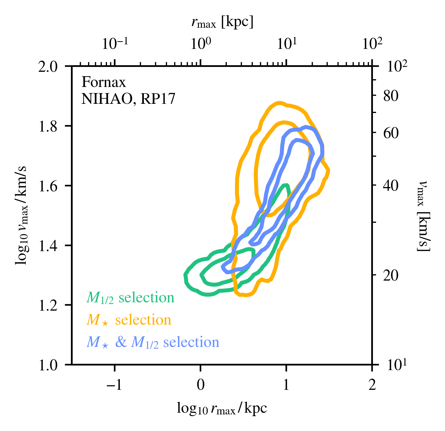
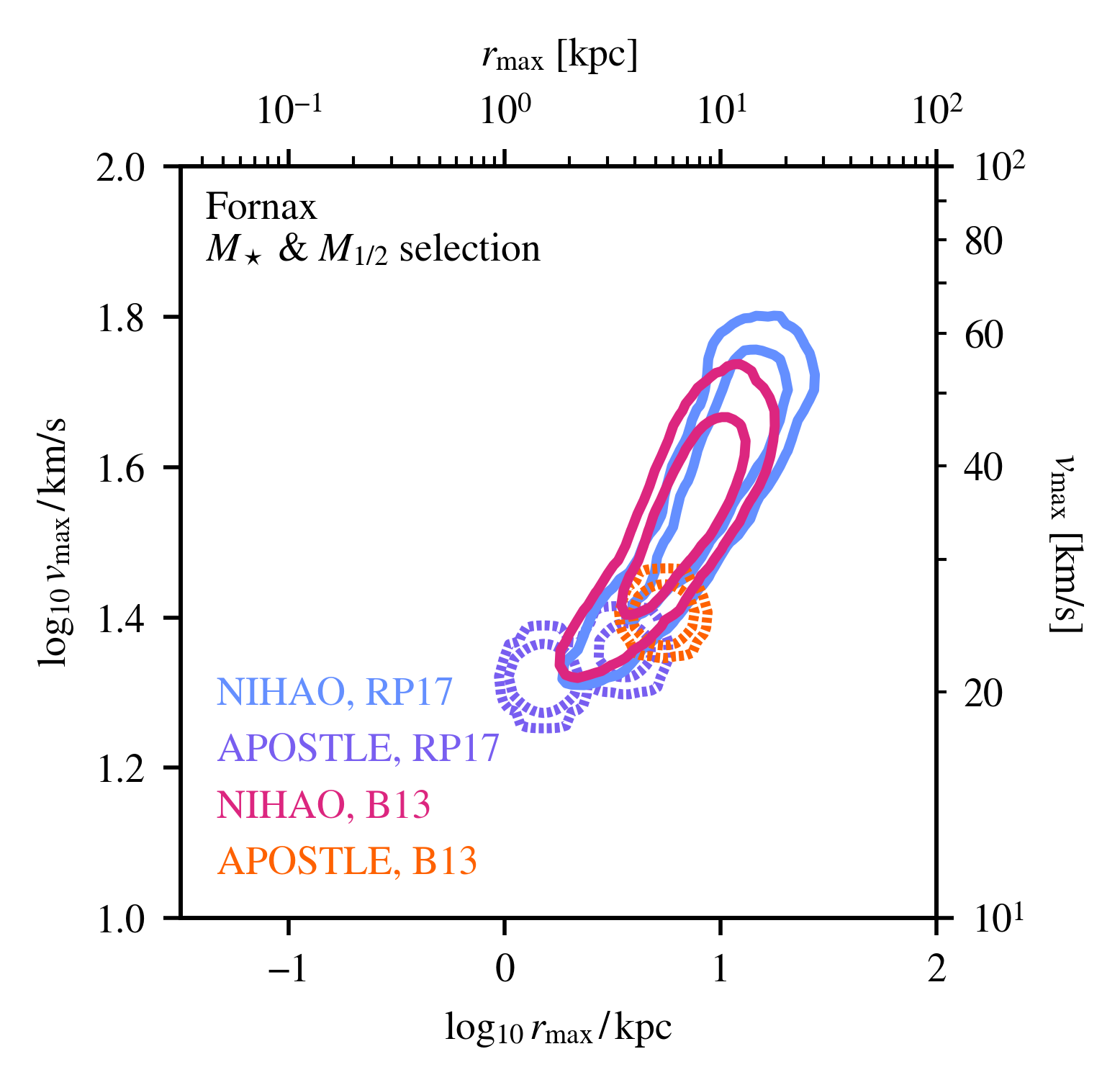
Figure 2: (Left) The inferred profile parameters $r_{\text{max}}$ and $v_{\text{max}}$ for the Fornax dwarf according to the procedure described in Section 2.2. The contours enclose 68 and 95% confidence regions based on the mass within the observed half-light radius ($M_{1/2}$, in green), the stellar mass ($M_{\star}$, in gold), and the combination of both parameters simultaneously (in blue). Observationally, Fornax has a fairly low $M_{1/2}$, leading this inference to be consistent both with the massive cored satellites and with smaller uncored satellites. Fornax’s stellar mass, on the other hand, is quite large, and selects only this former population. This selection is further refined by requiring that satellites simultaneously satisfy the observed $M_{1/2}$ and $M_{\star}$ values. The pericentric distance $r_{\mathrm{peri}}$ and infall time $t_{\mathrm{infall}}$ do not correlate strongly with $v_{\text{max}}$ or $r_{\text{max}}$ and are thus unable to constrain the space from the overall distribution of satellites; as such, they are not shown here. (Right) The combined inference from the left plot is shown under various models for baryonic feedback and the SMHM relation. The blue and magenta “NIHAO” contours assume strong feedback, while the purple and orange “APOSTLE” contours use a weaker model of baryonic feedback. The blue and purple contours assume the RP17 SMHM relation, which has a steeper faint-end slope than B13, taken for the magenta and orange contours. Notably, without the strong core formation of the NIHAO feedback emulator, the satellites consistent with both $M_{\star}$ and $M_{1/2}$ are much smaller, with lower $v_{\text{max}}$ and $r_{\text{max}}$. In both panels, the probability density is defined as a function of the base-ten logarithm of $r_{\text{max}}$ and $v_{\text{max}}$, not the quantities themselves, though $r_{\text{max}}$ and $v_{\text{max}}$ are provided on the top and right axes, respectively, for convenience. This convention is followed throughout this work. Furthermore, in this plot and throughout this work, we plot contours that are statistics-limited as dashed lines rather than complete contours. See Table 2 for more information.

Returning to the concrete example, consider the Fornax dwarf galaxy, whose mass and orbital parameters are provided in Table 1. The 68% confidence regions for these parameters are also indicated by the blue bands in Figure 1. In all the cases shown, the observed marginal distribution $f_{\,i}(\boldsymbol{\theta})$, which roughly corresponds to the width of the blue bands, is significantly smaller than the distribution $f_{\text{pred}}(\boldsymbol{\theta})$ obtained from SatGen, which corresponds to the spread of black points and contours. Only those satellites that fall in or near the blue band will contribute significantly to the weight $f_{\,i}(\boldsymbol{\theta})/f_{\text{pred}}(\boldsymbol{\theta})$ in Equation 2, shaping the resulting prediction for $f_{\,i}(\mathbf{x})$ with $\mathbf{x}=(r_{\text{max}},v_{\text{max}})$. While Figure 1 uses the NIHAO emulator and the RP17 SMHM relation, the SatGen sample can be easily run with different models to quantify the systematic effects on the inferred parameters. The next section works through this procedure for inferring $r_{\text{max}}$ and $v_{\text{max}}$ for Fornax and the other classical satellites.

3 Proof-of-Concept: Density Profile Inference

The technique described in Section 2 is very general and allows for the inference of arbitrary satellite parameters using any set of observables. This section applies the procedure to the specific case of modeling the profile parameters $(r_{\text{max}},\,v_{\text{max}})$, starting with the Fornax dwarf galaxy and later generalizing to other dwarfs. We examine a number of potential parameters that may constrain the halo profile and ultimately derive an inferred distribution for the profile parameters using the satellite’s stellar mass and its total mass within its half-light radius, discussing the systematic uncertainties on these results. These results agree well with analyses of stellar kinematics of MW dwarfs, as well as with a simple inference based on scaling relations such as abundance matching, though the uncertainties in these alternate methods are typically underestimated. Section 4 explores other galaxy properties beyond $(r_{\text{max}},\,v_{\text{max}})$ that can be inferred using this procedure.

Name	NIHAO RP17	APOSTLE, RP17	NIHAO, B13	APOSTLE, B13
Canes Venatici I	1341 (4083)	183 (706)	4988 (13571)	4546 (12922)
Carina	931 (7069)	19 (786)	9464 (22914)	3160 (15444)
Draco	4160 (11420)	1784 (5209)	1567 (4161)	3473 (9234)
Fornax	269 (832)	2 (4)	382 (1079)	1 (2)
Leo I	1351 (3766)	14 (216)	726 (2199)	660 (2506)
Leo II	2884 (7944)	393 (1341)	1880 (5203)	3144 (8699)
Sextans	1376 (4449)	217 (940)	4952 (13468)	4760 (13312)
Sculptor	1397 (3863)	244 (867)	672 (1846)	1502 (4148)
Ursa Minor	1715 (5235)	276 (970)	3045 (8163)	3618 (9866)

Table 2: This table contains the number of SatGen satellites comprising 68% (95%) of the weight in the $M_{\star}-M_{1/2}$ combined inference for the models considered in this work. The models vary over all combinations of the feedback emulator (NIHAO versus APOSTLE) and the SMHM relation (RP17 versus B13). A lower number indicates that there are few satellites in the SatGen sample that appropriately reproduce the $M_{\star}$ and $M_{1/2}$ measurements for the dwarf, leading to a small number of high-weighted satellites driving the 68% or 95% containment regions of the inference. For example, in the APOSTLE emulator with RP17 SMHM relation, there are two satellites that most closely resemble Fornax that furnish $\geq 68\%$ of the weight used to perform inferences, since there are few SatGen satellites able to match both the $M_{\star}$ and the $M_{1/2}$ of Fornax in this model. We highlight the dwarfs for which fewer than 25 SatGen satellites contribute to the inference. This threshold is an arbitrary choice, but it indicates those dwarfs for which the inference is subject to low statistics, despite the large sample of MWs (4,000 for the NIHAO RP17 dataset and 2,000 for the other three). In all figures, the inferences corresponding to bolded numbers in this table are distinguished (via dashed-line contours) from the inferences driven by more than 25 SatGen satellites.

3.1 Profile Inference for Fornax-like Galaxies

Figure 1 shows four observables that can potentially correlate with the halo profile of a Fornax-like galaxy: the stellar mass $M_{\star}$, the mass $M_{1/2}$ within the observed half-light radius $r_{1/2}$, the pericentric distance $r_{\mathrm{peri}}$, and the infall time $t_{\mathrm{infall}}$. The figure panels illustrate the strength of these correlations across the sample of SatGen realizations of MW-like galaxies. In general, the orbital parameters $r_{\mathrm{peri}}$ and $t_{\mathrm{infall}}$ do not correlate very strongly with either $r_{\text{max}}$ or $v_{\text{max}}$ and are thus not expected to have much constraining power. In contrast, the parameters $M_{1/2}$ and $M_{\star}$ exhibit strong correlations with the halo parameters $r_{\text{max}}$ and $v_{\text{max}}$, and therefore they are expected to provide substantial constraining power when inferring, e.g., the joint distribution function of $r_{\text{max}}$ and $v_{\text{max}}$. In particular, the correlation between $v_{\text{max}}$ and $M_{\star}$ is monotonic with little scatter, reflecting the fact that larger galaxies reside in larger halos. $M_{1/2}$ is also tightly correlated with $v_{\text{max}}$, although the relation exhibits a turnover at the higher-mass end. This turnover reflects the feedback prescription: the NIHAO emulator efficiently cores satellites with a large stellar-to-halo mass ratio, which increases for larger subhalos according to the SMHM relation. As such, at the $M_{1/2}$ of Fornax (indicated by the blue shaded region), there is a population of both low-$v_{\text{max}}$ halos and high-$v_{\text{max}}$ halos, where the former population is comprised of smaller galaxies with low $M_{\star}$ and $M_{1/2}$ and the latter population is comprised of galaxies with larger $M_{\star}$ that correspondingly are cored to lower $M_{1/2}$. In the APOSTLE emulator, where feedback is less efficient, this effect is not present, and the $M_{1/2}$ – $v_{\text{max}}$ relation remains monotonic across the entire parameter space.

The technique of Section 2.2 leverages these correlations to infer the distribution of $\mathbf{x}=(r_{\text{max}},\,v_{\text{max}})$. The left panel of Figure 2 shows 68% and 95% containment regions for $f_{\,i}(\mathbf{x}{})$ in the 2D $r_{\text{max}}$ – $v_{\text{max}}$ plane for the Fornax dwarf galaxy, highlighting the differences in choice of the known parameter $\boldsymbol{\theta}$. Gold and green contours correspond to $\boldsymbol{\theta}=M_{\star}$ and $\boldsymbol{\theta}=M_{1/2}$, respectively, while blue contours correspond to the joint $\boldsymbol{\theta}=(M_{\star},\,M_{1/2})$. Using $\boldsymbol{\theta}{}=M_{\star}$, the inferred $\mathbf{x}$ values are $r_{\text{max}}={8.21}_{-3.11}^{+4.54}$ kpc and $v_{\text{max}}={45.36}_{-11.96}^{+9.30}$ km/s, occupying a large region of the parameter space shown in Figure 2. In contrast, the tight scatter in the individual relation between $M_{1/2}$ and $v_{\text{max}}$ leads to a smaller preferred region of parameter space when $\boldsymbol{\theta}=M_{1/2}$. However, as mentioned above, the fixed $M_{1/2}$ window corresponding to the Fornax measurement contains both smaller satellites and larger satellites that have been cored to reach that $M_{1/2}$ value. This results in generally smaller inferred values of $v_{\text{max}}={21.09}_{-1.54}^{+2.70}$ km/s with a tail that extends to the larger cored systems. Said differently, the low $M_{1/2}$ value of Fornax points to the likely existence of a relatively small DM halo. However, another possibility allowed by strong feedback (such as that of the NIHAO emulator) is a much larger DM halo that has been efficiently cored to explain the low $M_{1/2}$ measurement. The inference derived using the joint $\boldsymbol{\theta}=(M_{\star},\,M_{1/2})$ corresponds to $r_{\text{max}}={10.36}_{-4.56}^{+4.25}$ kpc and $v_{\text{max}}={40.53}_{-11.36}^{+8.80}$ km/s; selecting on $M_{\star}$ and $M_{1/2}$ simultaneously removes the smaller region of parameter space preferred by $M_{1/2}$ alone while improving the uncertainty of using $M_{\star}$ alone.

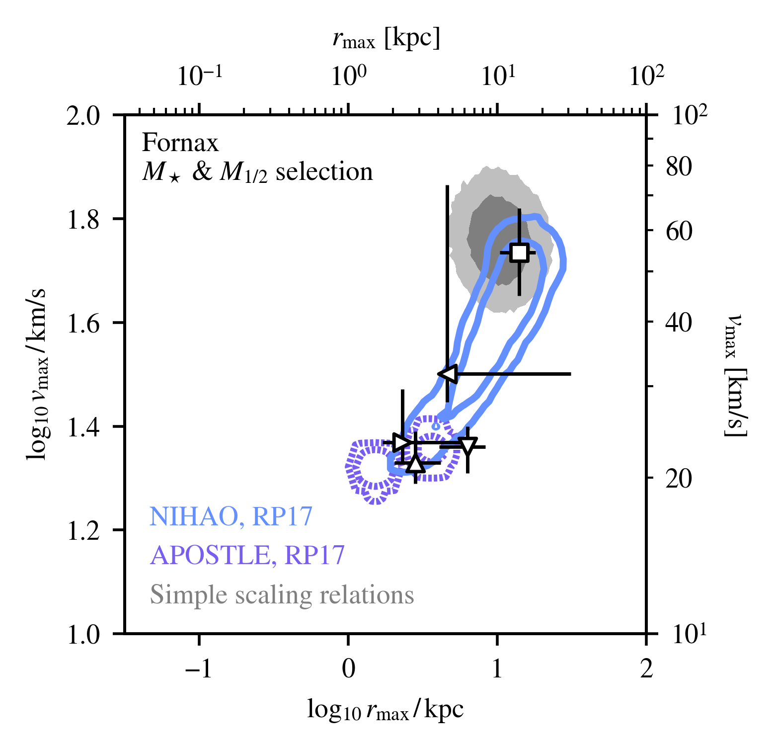
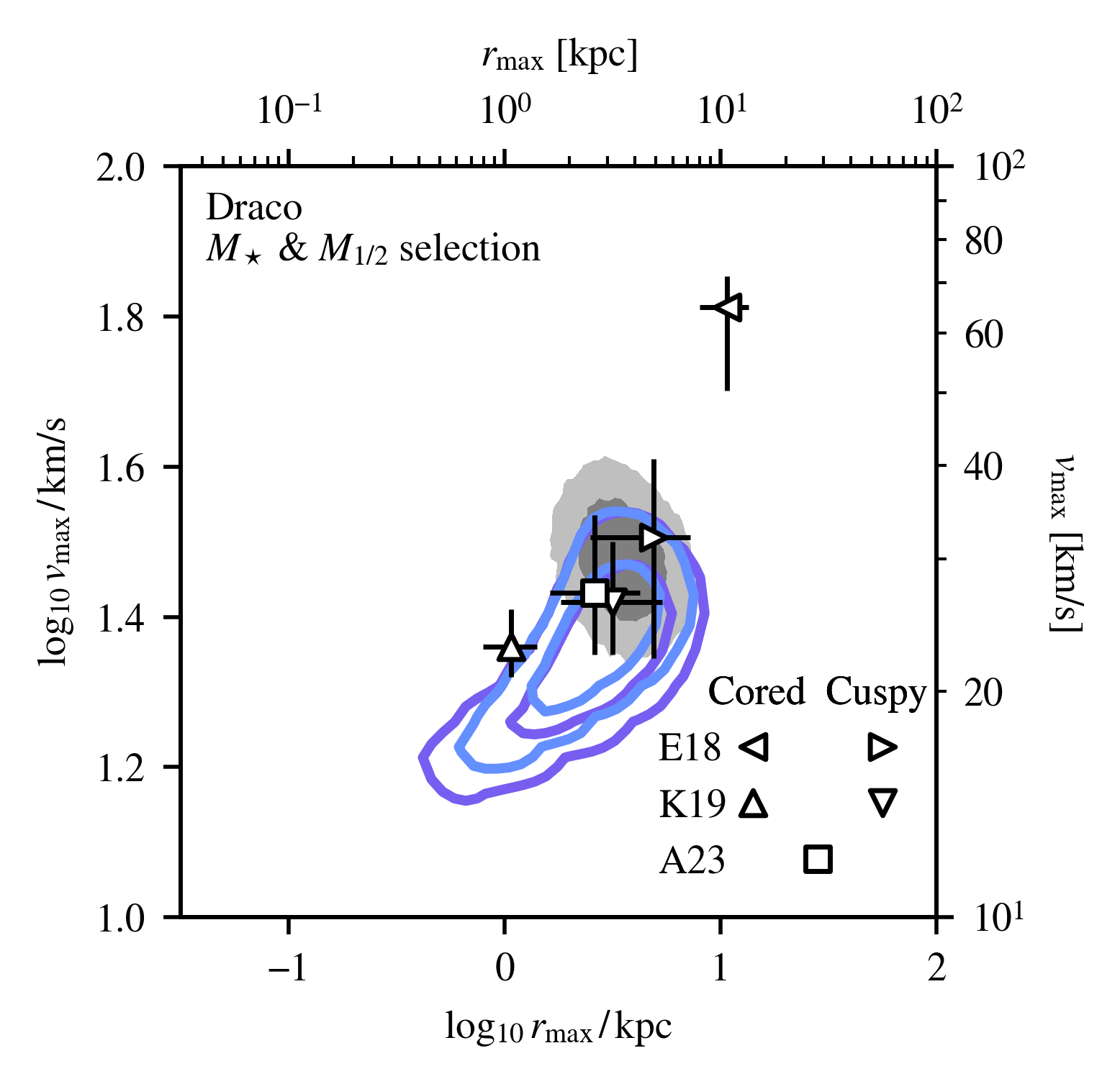
Figure 3: This figure shows the results of the SatGen analysis for the Fornax (left) and Draco (right) dwarfs, assuming the RP17 SMHM relation and varying over feedback emulation, as compared with other results from the literature. Data points are kinematic measurements, including E18, shown in leftward- and rightward-pointing triangles; K19, shown in upward- and downward-pointing triangles; and A23, shown as a square. For the first two models, the direction of the triangle indicates the assumption of a cored or cuspy DM profile respectively, while A23 models the DM halo with a profile where the inner slope is allowed to vary; the other two analyses model the DM halo with both a cuspy profile and a cored profile. Additionally, we compare these results to the prediction obtained by the simple scaling relations of the RP17 SMHM relation and the concentration–mass relation from Moliné et al. (2023). The SatGen inference is generally in agreement with these analyses, particularly due to the highly correlated and non-Gaussian errors in the observational analyses. For results on the other dwarfs, see Figure 8.

The analysis performed in this section is contingent on the assumption that the population of SatGen satellites accurately models the population of MW satellites, but there are a number of systematic uncertainties that influence the underlying distribution. Two important sources of modeling uncertainty are the feedback model and the SMHM relation, including their combined effects on each other. As described previously, SatGen can be tuned to emulate baryonic feedback from either the NIHAO (Wang et al., 2015) or APOSTLE (Sawala et al., 2016) simulations, and it can incorporate an SMHM relation based on either RP17 or B13. Modifying either of these aspects of the model leads to different overall populations of satellites and thus potentially different inferences for $r_{\text{max}}$ and $v_{\text{max}}$. The right panel of Figure 2 shows how the combined $M_{\star}$ – $M_{1/2}$ inference varies for all four combinations of the two SMHM and two feedback prescriptions. Note that dashed contours in this figure correspond to inferences which are set by a small number of highly-weighted SatGen satellites, and thus should be interpreted with caution. Specifically, if fewer than 25 SatGen satellites comprise $\geq 68\%$ of the total weight, then the 68% containment contour is dashed, and similarly for the 95% contour.

A main distinction between the four inferred distributions is the difference between the two corresponding to the NIHAO feedback emulator and the two corresponding to the APOSTLE feedback emulator. Qualitatively, the NIHAO emulator (which provides stronger feedback than APOSTLE) pushes the contours to larger values of both $v_{\text{max}}$ and $r_{\text{max}}$. This occurs for reasons that depend on both the $M_{\star}$ and the $M_{1/2}$ requirements. First, Fornax has a sizable $M_{\star}$, which can produce strong feedback in general, and even more so with the NIHAO emulator. Therefore, simultaneously matching Fornax’s large $M_{\star}$ and relatively low $M_{1/2}$ corresponds to either smaller and cuspier halos that occur naturally with APOSTLE, or larger and more cored halos, which occur naturally with NIHAO. However, this difference between NIHAO and APOSTLE is also partially driven by low statistics. Due to the lack of cored satellites in the APOSTLE emulator, it is unlikely for a satellite to satisfy both the observed $M_{\star}$ and $M_{1/2}$ simultaneously. Finally, for a given stellar mass, the B13 SMHM relation prefers satellites with less massive DM halos than does the RP17 SMHM relation. However, varying the SMHM relation has only a mild effect on the shapes and positions of the contours for both feedback prescriptions.

3.2 Comparisons to Observations

In the previous section, the analysis and systematics were described for the case of Fornax. Below, the scope is broadened to the rest of the classical satellites. Table 3 provides the median inferred $r_{\text{max}}$ and $v_{\text{max}}$ values (together with 65% containment intervals) for the nine bright MW spheroidal dwarfs considered in this work and for all four combinations of feedback prescriptions and SMHM relations. The feedback models and choice of SMHM relation affect the broader population in much the same way as described for the Fornax example above, although there is less extreme tension between $M_{1/2}$ and $M_{\star}$ for these satellites and thus higher statistics for all four combinations. The 2D $r_{\text{max}}-v_{\text{max}}$ plots for these nine systems are shown in Figure 8 for $\boldsymbol{\theta}=(M_{\star},\,M_{1/2})$, assuming RP17 for both the NIHAO and APOSTLE emulators. Additionally, the specific examples of the Fornax and Draco dwarfs are shown in Figure 3.

	NIHAO, RP17		APOSTLE, RP17		NIHAO, B13		APOSTLE, B13
Name	$r_{\text{max}}$ [kpc]	$v_{\text{max}}$ [km/s]	$r_{\text{max}}$ [kpc]	$v_{\text{max}}$ [km/s]	$r_{\text{max}}$ [kpc]	$v_{\text{max}}$ [km/s]	$r_{\text{max}}$ [kpc]	$v_{\text{max}}$ [km/s]
Canes Venatici I	${2.68}_{-1.74}^{+3.09}$	${16.97}_{-3.50}^{+5.39}$	${1.02}_{-0.46}^{+5.35}$	${13.94}_{-1.29}^{+7.18}$	${2.01}_{-0.63}^{+0.94}$	${16.55}_{-1.81}^{+1.95}$	${1.84}_{-0.64}^{+0.91}$	${15.00}_{-1.33}^{+1.59}$
Carina	${4.48}_{-3.26}^{+4.36}$	${21.60}_{-9.23}^{+4.06}$	${6.67}_{-5.68}^{+1.83}$	${22.74}_{-9.01}^{+2.86}$	${2.49}_{-0.84}^{+1.16}$	${17.74}_{-3.03}^{+3.42}$	${2.59}_{-1.06}^{+1.41}$	${15.38}_{-2.74}^{+2.89}$
Draco	${2.72}_{-0.97}^{+1.22}$	${23.49}_{-3.36}^{+3.47}$	${2.77}_{-1.30}^{+1.44}$	${22.30}_{-3.85}^{+3.87}$	${1.99}_{-0.69}^{+1.05}$	${21.63}_{-2.46}^{+2.82}$	${1.74}_{-0.61}^{+0.96}$	${19.60}_{-1.88}^{+2.31}$
Fornax	${10.36}_{-4.56}^{+4.25}$	${40.53}_{-11.36}^{+8.80}$	${1.74}_{-0.39}^{+2.01}$	${21.41}_{-3.03}^{+3.53}$	${7.03}_{-2.64}^{+3.29}$	${34.65}_{-7.50}^{+8.48}$	${5.40}_{-0.84}^{+0.99}$	${25.21}_{-3.03}^{+3.44}$
Leo I	${5.39}_{-1.86}^{+2.39}$	${35.98}_{-7.97}^{+7.76}$	${7.40}_{-3.19}^{+2.67}$	${35.80}_{-9.19}^{+5.83}$	${3.79}_{-1.33}^{+1.98}$	${31.24}_{-5.78}^{+6.56}$	${4.13}_{-1.51}^{+2.26}$	${26.00}_{-4.46}^{+5.58}$
Leo II	${3.62}_{-1.47}^{+1.69}$	${25.97}_{-5.63}^{+4.99}$	${4.38}_{-2.22}^{+1.71}$	${26.56}_{-7.70}^{+4.79}$	${2.40}_{-0.87}^{+1.26}$	${22.67}_{-3.60}^{+3.86}$	${2.19}_{-0.69}^{+1.12}$	${19.21}_{-2.71}^{+3.04}$
Sextans	${2.49}_{-1.49}^{+3.42}$	${17.25}_{-2.71}^{+5.03}$	${1.05}_{-0.44}^{+4.16}$	${15.04}_{-1.13}^{+4.55}$	${2.10}_{-0.68}^{+0.99}$	${17.07}_{-1.58}^{+1.87}$	${1.88}_{-0.66}^{+0.96}$	${15.87}_{-1.17}^{+1.44}$
Sculptor	${4.35}_{-1.53}^{+1.80}$	${31.74}_{-6.02}^{+5.84}$	${5.02}_{-2.93}^{+2.30}$	${29.81}_{-8.34}^{+5.99}$	${3.07}_{-1.06}^{+1.74}$	${28.62}_{-4.32}^{+5.02}$	${2.83}_{-0.95}^{+1.50}$	${24.02}_{-3.08}^{+3.66}$
Ursa Minor	${3.58}_{-2.20}^{+1.83}$	${21.10}_{-5.35}^{+4.08}$	${2.63}_{-1.95}^{+3.17}$	${17.78}_{-3.77}^{+6.58}$	${2.02}_{-0.64}^{+1.02}$	${18.60}_{-2.10}^{+2.45}$	${1.88}_{-0.62}^{+0.91}$	${16.63}_{-1.55}^{+1.82}$

Table 3: The SatGen $r_{\text{max}}$ – $v_{\text{max}}$ inference for the nine bright MW spheroidal dwarfs. From left to right, this table contains the name of the satellite, the inferred $r_{\text{max}}$, and the inferred $v_{\text{max}}$, with 16th, 50th, and 84th percentiles reported, for each of the four models considered. The four models vary over all combinations of the feedback emulator (NIHAO versus APOSTLE) and the SMHM relation (RP17 versus B13). For a comparison to observations, see Figure 3 and Figure 8. These inferences are performed independently as one-dimensional inferences, where the quantiles are well-defined and are not subject to the choice of logarithmic versus non-logarithmic coordinates described in the caption of Figure 2.

As a point of comparison to the contours inferred by using SatGen, one can rely on a combination of empirical scaling relations as a simple way to directly infer a similar distribution in the $r_{\text{max}}$ – $v_{\text{max}}$ plane. In particular, the total stellar mass $M_{\star}$ has long been used in abundance matching studies to infer a DM halo mass from stellar observations (Kravtsov et al., 2004). Along with a concentration–mass relation, this is enough to specify a standard two-parameter halo such as the Navarro-Frenk-White (NFW) profile (Navarro et al., 1997). The grey shaded regions in Figure 3 correspond to our inference of the distribution using such a technique. This simple inference agrees fairly well with the colored contours (those that are not statistics-limited), as is also illustrated for the full sample of classical satellites in Figure 8.

These simple grey distributions assume the RP17 model as well as the Moliné et al. (2023) position-dependent concentration–mass relation for subhalos, which provides a simple fit to account for the orbital evolution of a satellite’s density profile. The SMHM relation is assumed not to change after infall. However, this is inaccurate for a number of reasons. Most importantly, tidal stripping removes DM halo mass from the outside inwards, while stellar mass is generally maintained (except in the most disrupted halos). Consequently, the simple scaling relations (grey colored region) miss allowed regions of lower-mass halos, which are properly included when using the SatGen formalism (colored contours). Since the SatGen inference also includes information on the $M_{1/2}$ of the satellites, the most probable regions are shifted from the simple scaling relation prediction, particularly for the case of Fornax, which has an $M_{1/2}$ that tends to prefer lower-mass halos, as mentioned above. On the other hand, for other satellites (e.g., Draco) the $M_{1/2}$ and $M_{\star}$ SatGen inferences agree both with each other and with the simple scaling relation-based inference.

However, the spread in the distributions in all cases are significantly different: SatGen provides realistic, correlated errors, while the simple scaling relation inferences are somewhat more naïve in their shape and extent. The uncertainties in the simple scaling relation inference technique come from the intrinsic scatter in the SMHM relation and in the mass-concentration relation. In determining the grey regions in the figure, the Moliné et al. (2023) mass-concentration relation has been given a scatter of 0.33 dex, based on conclusions drawn in the earlier Moliné et al. (2017) model. This simple, uncorrelated treatment of uncertainties tends to underestimate the extent and shape of the uncertainties found through the SatGen technique—such simple estimations ignore the complex nonlinear evolution satellites undergo.

The two types of $r_{\text{max}}{}$ – $v_{\text{max}}{}$ inferences described above (using SatGen and simple scaling relations) can also be compared to previous studies in the literature that use internal kinematic data to constrain $r_{\text{max}}{}$ and $v_{\text{max}}{}$. The points with error-bars in Figure 3 show the results of analyses performed by Errani et al. (2018, hereafter E18), Kaplinghat et al. (2019, K19), and Andrade et al. (2023, A23). The data points generally align with the SatGen inference, and their spread tends to correlate between $r_{\text{max}}$ and $v_{\text{max}}$ in roughly the same way. The scatter between these observational measurements is often large, suggesting sensitivity to untreated systematic uncertainties in the observational models. This is especially true for Leo II and Ursa Minor (see Figure 8), where these observational fits have large scatter and poor agreement with each other, particularly in $r_{\text{max}}{}$.

The large scatter is likely due, at least in part, to the different approaches used to model the DM halo profile and the stellar velocity anisotropy and density. The profile shapes assumed in each analysis vary somewhat: E18 and K19 both perform Jeans analyses under the assumption of two different DM density profiles, one of which is cored with a flat inner slope and one of which is cuspy with an inner profile of $\rho\propto r^{-1}$, though the exact functional forms used in each study differ. A23 uses a distribution function modeling approach that assumes a profile shape with a flexible inner slope, allowing for the fitting procedure to choose an optimal value. Evidently, the different approaches and assumptions of each study greatly affect the results, which can lead to disagreement with the flexible SatGen-based inference.

By sampling over feedback models, the SatGen analysis allows for variation in the inner slope. In general, the slopes of the inferred profiles from SatGen lie between $\rho\propto r^{-0.5}$ and $r^{-2}$, with the notable exception of Fornax, which is consistent with even shallower slopes in the NIHAO feedback emulator. For each dwarf, the NIHAO feedback emulator prefers a more cored slope than the APOSTLE emulator, which is to be expected. Figure 9 shows the distribution of inferred inner slopes for each of the classical dwarfs considered in this study.

4 Inference of Additional Properties

As shown in Section 3, the method presented in this work allows for the inference of the structural properties of DM halos based on the stellar mass of the satellite galaxies they host, and this inference can be performed efficiently over many models of baryonic physics and galaxy formation. The inference also agrees with other observational models of the structural properties, even though it does not utilize this information to perform the inference. Below, we extend the applications of the method beyond internal properties of the classical satellites, leveraging the assembly history data provided by the SatGen model. In particular, we infer the relation between the central densities and pericenters of the classical satellites, as well as their association with a larger group of subhalos at their accretion time.

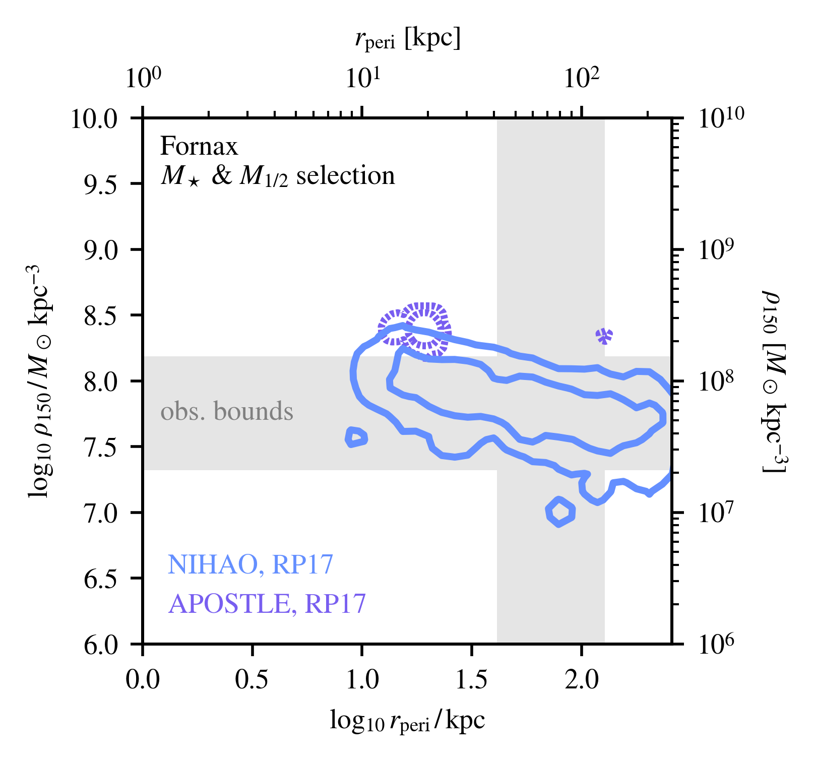
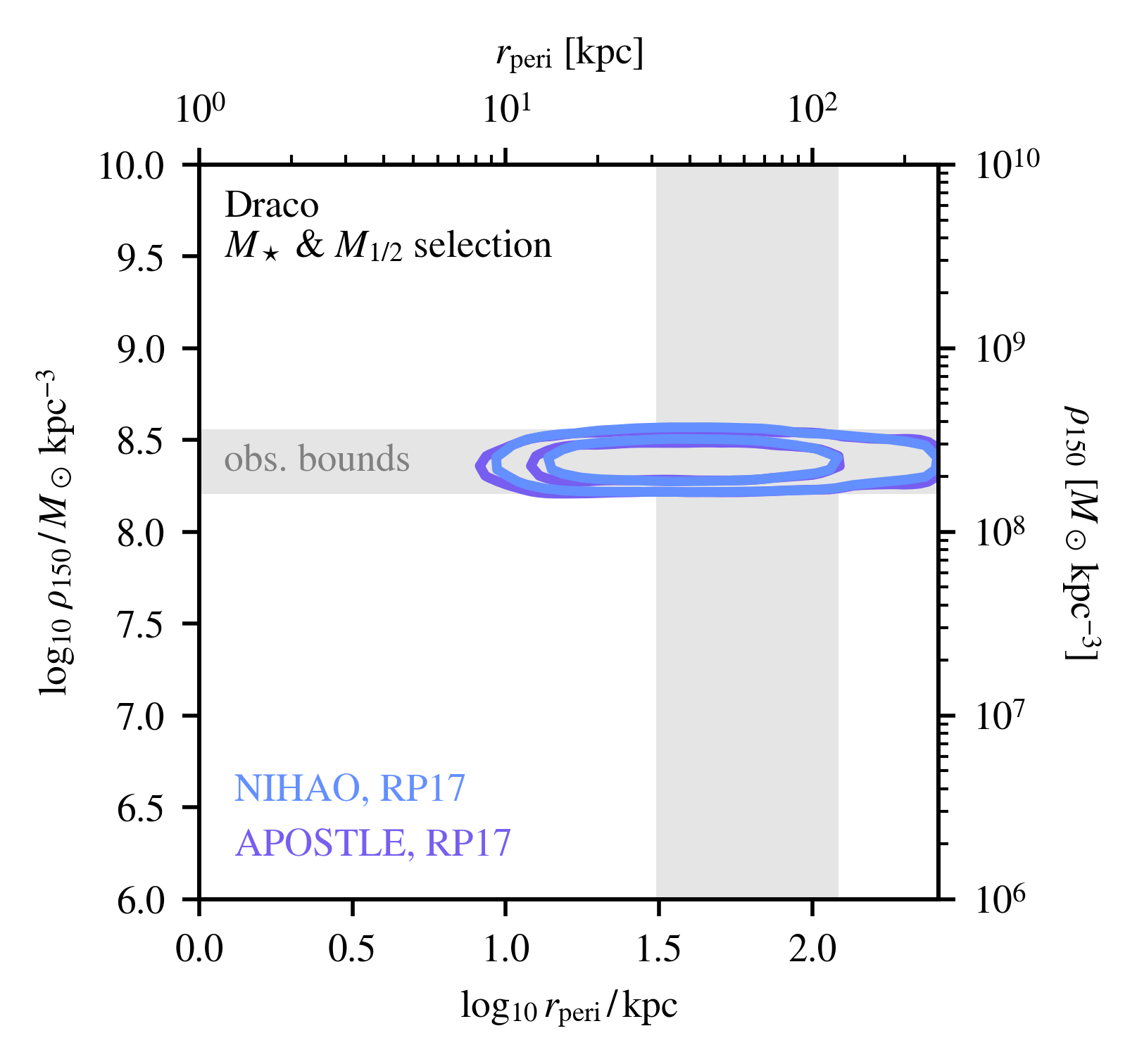
Figure 4: 68 and 95% confidence intervals for the pericenter $r_{\mathrm{peri}}$ and central density $\rho_{\mathrm{150}}$ of Fornax (left) and Draco (right), based on the combined $M_{\star}$ and $M_{1/2}$-based inference. The bands represent the maximum and minimum one-sigma observational results for Fritz et al. (2018), Battaglia et al. (2022), and Pace et al. (2022) for $r_{\mathrm{peri}}$; and Read et al. (2019), Kaplinghat et al. (2019), and Hayashi et al. (2020) for $\rho_{150}$, marginalizing over all MW potentials in the pericenter modeling and all assumed profiles (including both cusps and cores) in the density modeling. The SatGen results assume the RP17 model and are shown for both the NIHAO and APOSTLE feedback emulators (in blue and purple, respectively). In the case of Fornax, the satellites able to match both masses in the NIHAO feedback emulator also match the observed low central density and fairly large pericenter—Fornax-like satellites do not remain Fornax-like with low pericenters. Conversely, the APOSTLE feedback emulator requires the tidal stripping enhancement of a low pericenter to match both mass constraints, which brings it in slight tension with observations. Unlike Fornax, the high central density of Draco can be achieved in either feedback emulator, and satellites that match the observed masses also satisfy observational limits on the central density and pericenter.

4.1 Central Density – Pericenter Relations

An advantage of the semi-analytic orbit integration approach is that it not only provides access to the internal properties of the SatGen satellites, but also to their orbital properties. This allows for the inference of reasonable orbital distributions of these satellites. This inference is grounded in a formalism that does not suffer from the numerical artifacts impacting studies of numerical simulations: the semi-analytic approach allows one to track the satellites in arbitrary environments, without issues such as artificial disruption or low resolution. Additionally, simulations struggle to resolve satellites in high-density environments, e.g. at their orbital pericenters, but this is also where dynamical effects are most important. SatGen self-consistently accounts for these effects, allowing for investigation of the interplay between orbital trajectory and resultant subhalo profile.

SatGen allows for the presence of a disk potential in the orbit integration, which causes more tidal mass loss near pericenter, an effect that is enhanced for smaller pericenters and lower concentrations (Green et al., 2022). The halo profile reacts to the DM mass loss as the subhalo evolves on the Errani et al. (2018) tidal tracks, causing the structural parameters to evolve throughout the orbit. We choose to examine this evolution in terms of the central density at 150 pc, denoted $\rho_{150}$, which may posses some dependence on the orbital trajectory, particularly in the lowest-concentration halos that are most affected by tides. This is particularly interesting for the case of Fornax, which many lines of argument suggest to have a low-density dark matter core (e.g., Cole et al. (2012); Jardel & Gebhardt (2012); Kowalczyk et al. (2019), though see Boldrini et al. (2019); Meadows et al. (2020); Genina et al. (2022) for some caveats to these arguments). As is demonstrated below, the interplay of central density and orbital pericenter, $r_{\mathrm{peri}}$, can provide critical insight into the specific feedback model.

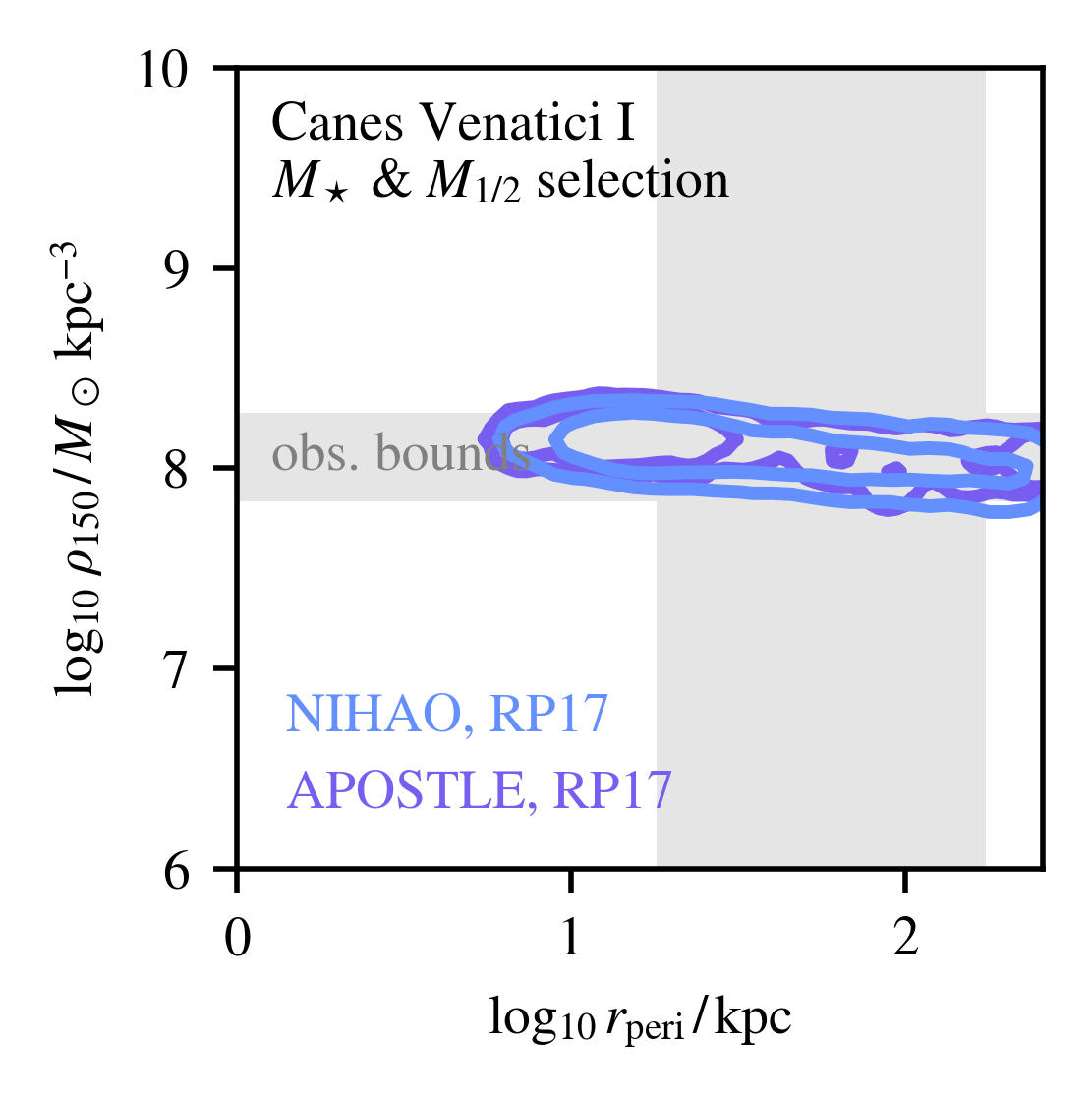
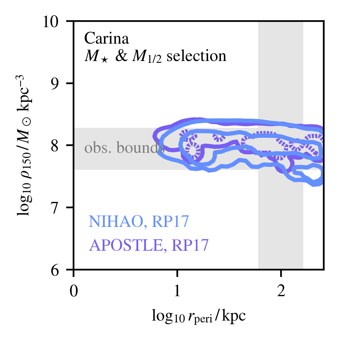
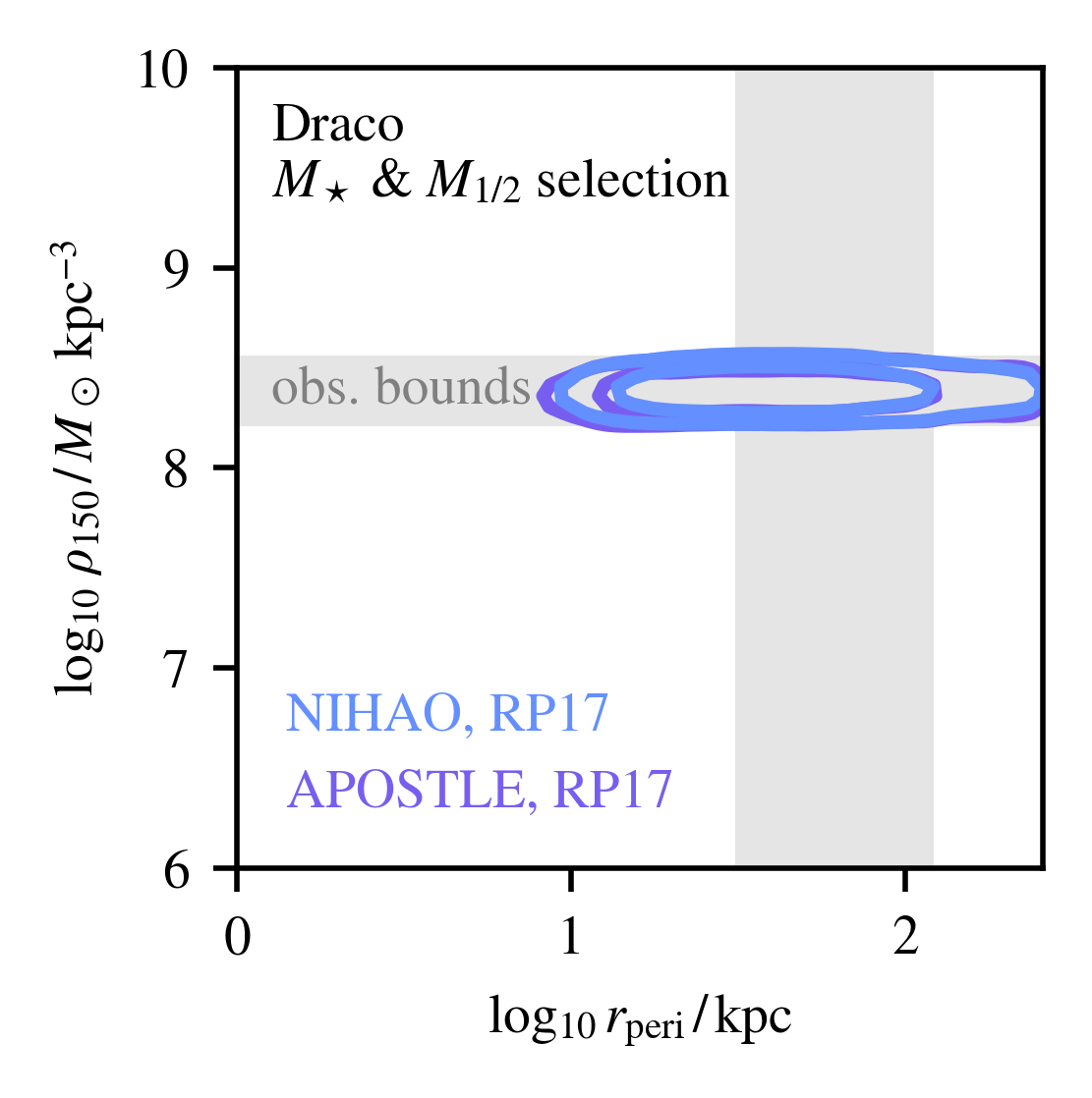
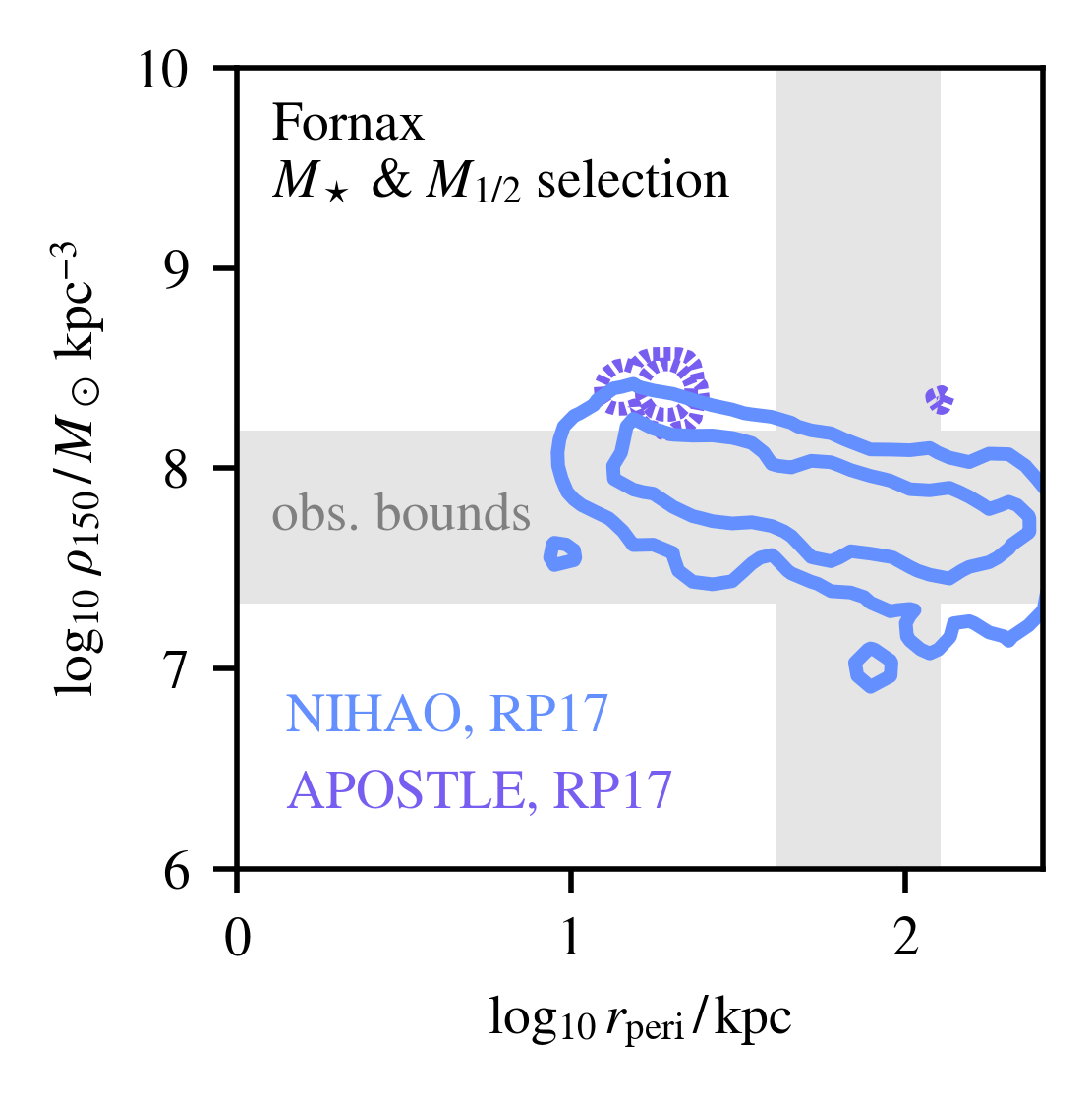
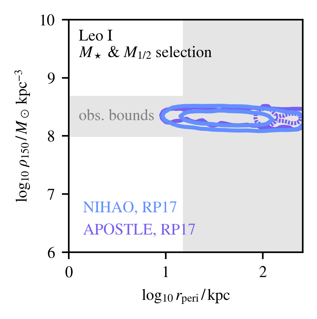
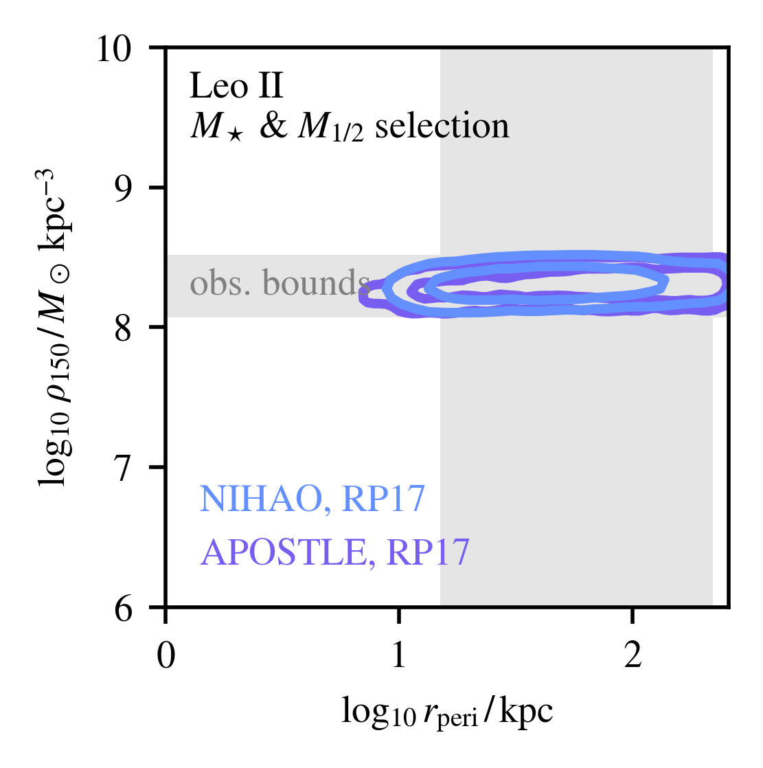
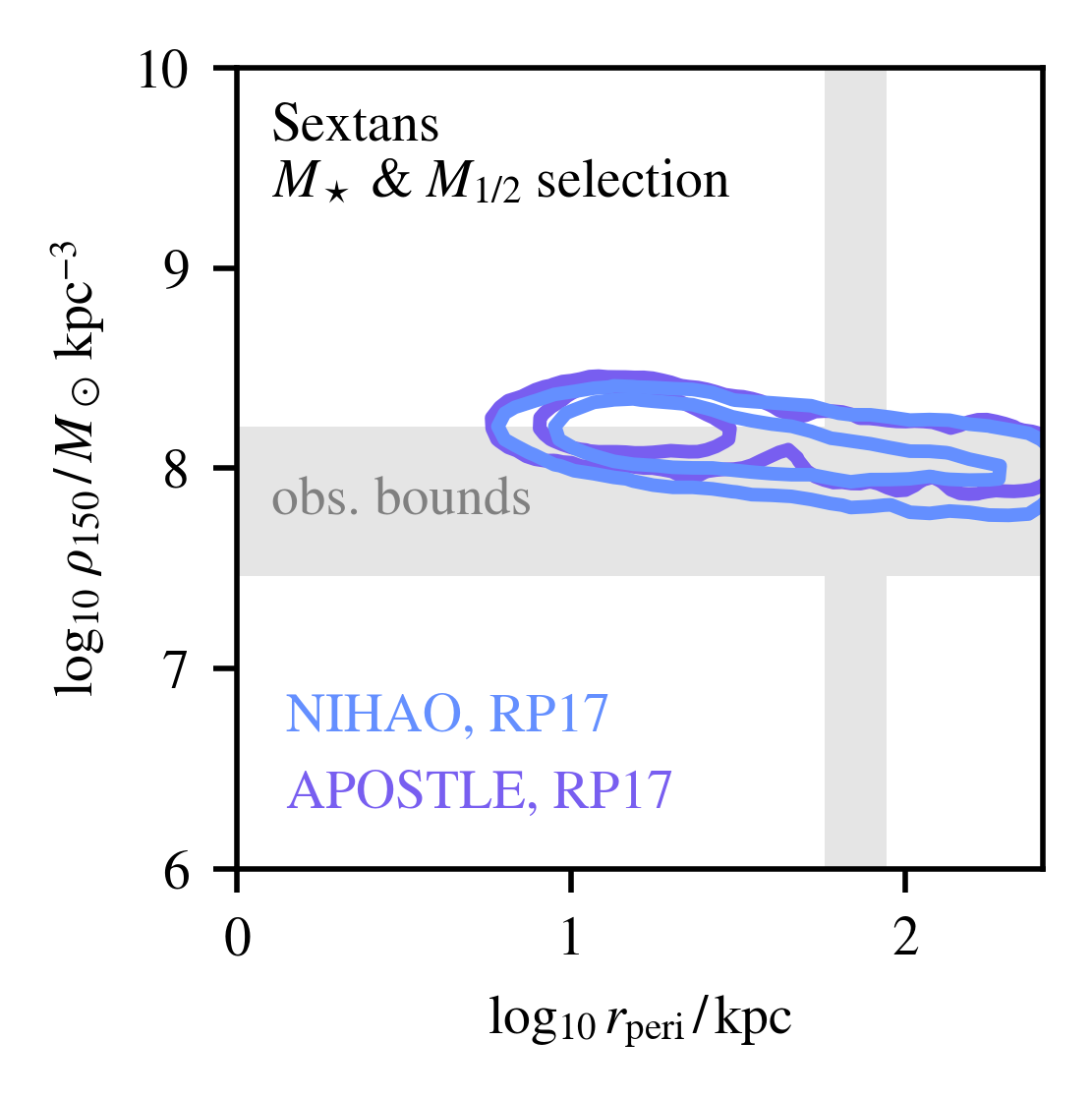
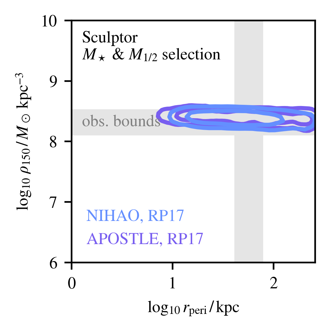
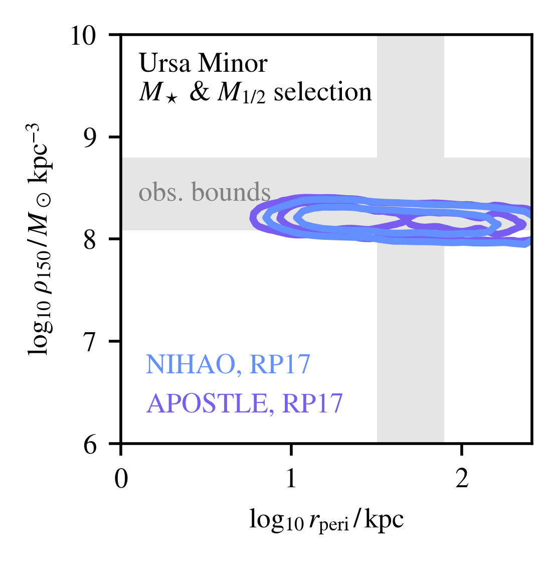
Figure 11: A version of Figure 4 for all classical satellites. Notably, the inference for $\rho_{150}$ is generally consistent with observation, though Sextans prefers the denser side of the observed region and Ursa Minor the less dense side.

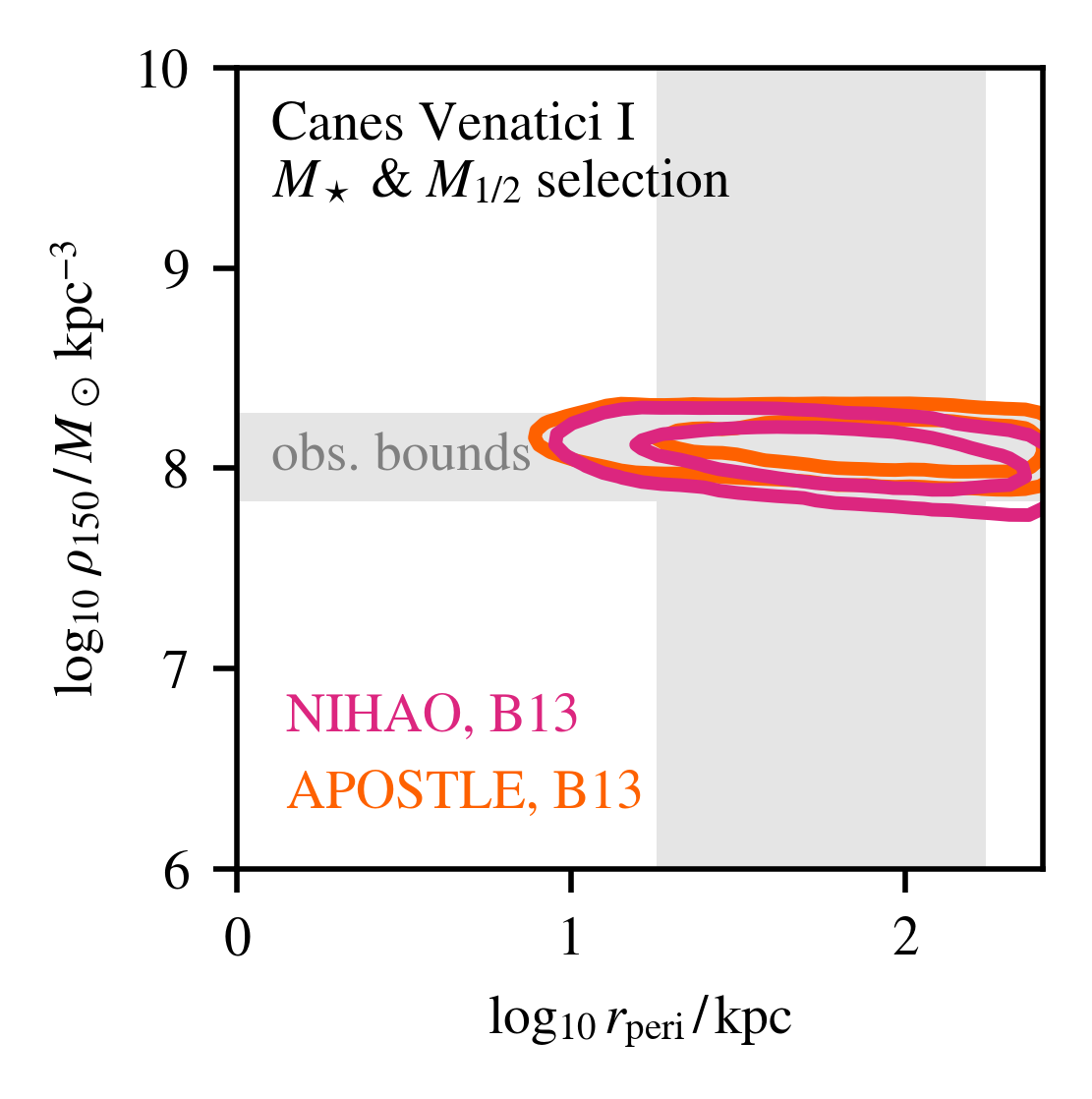
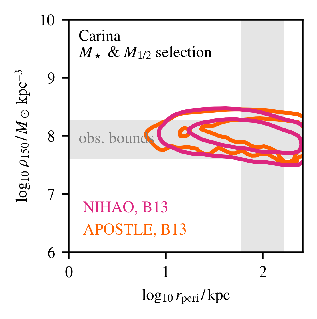
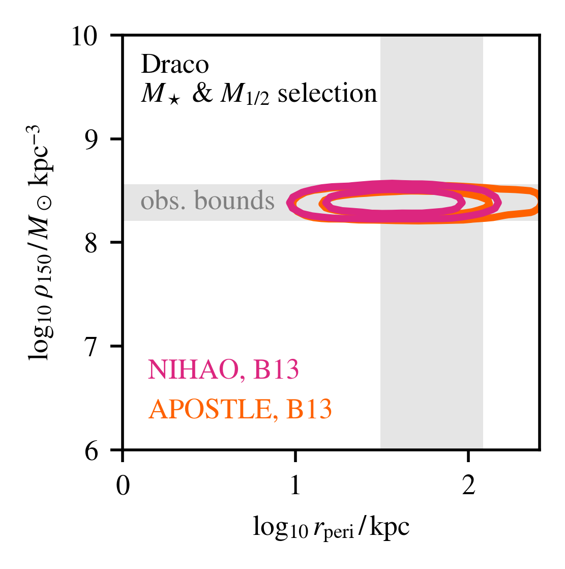
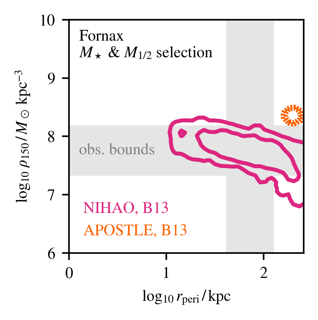
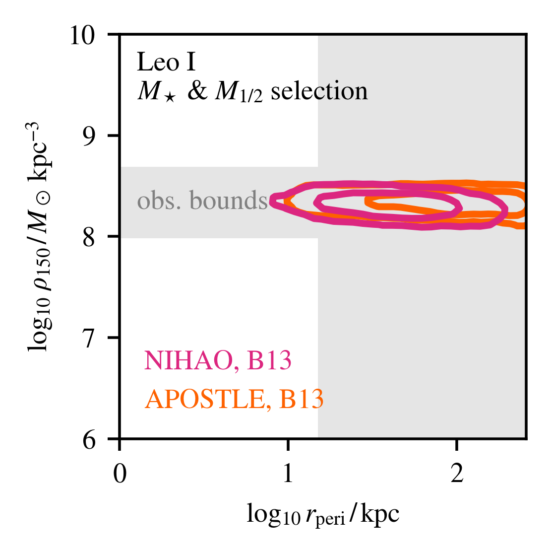
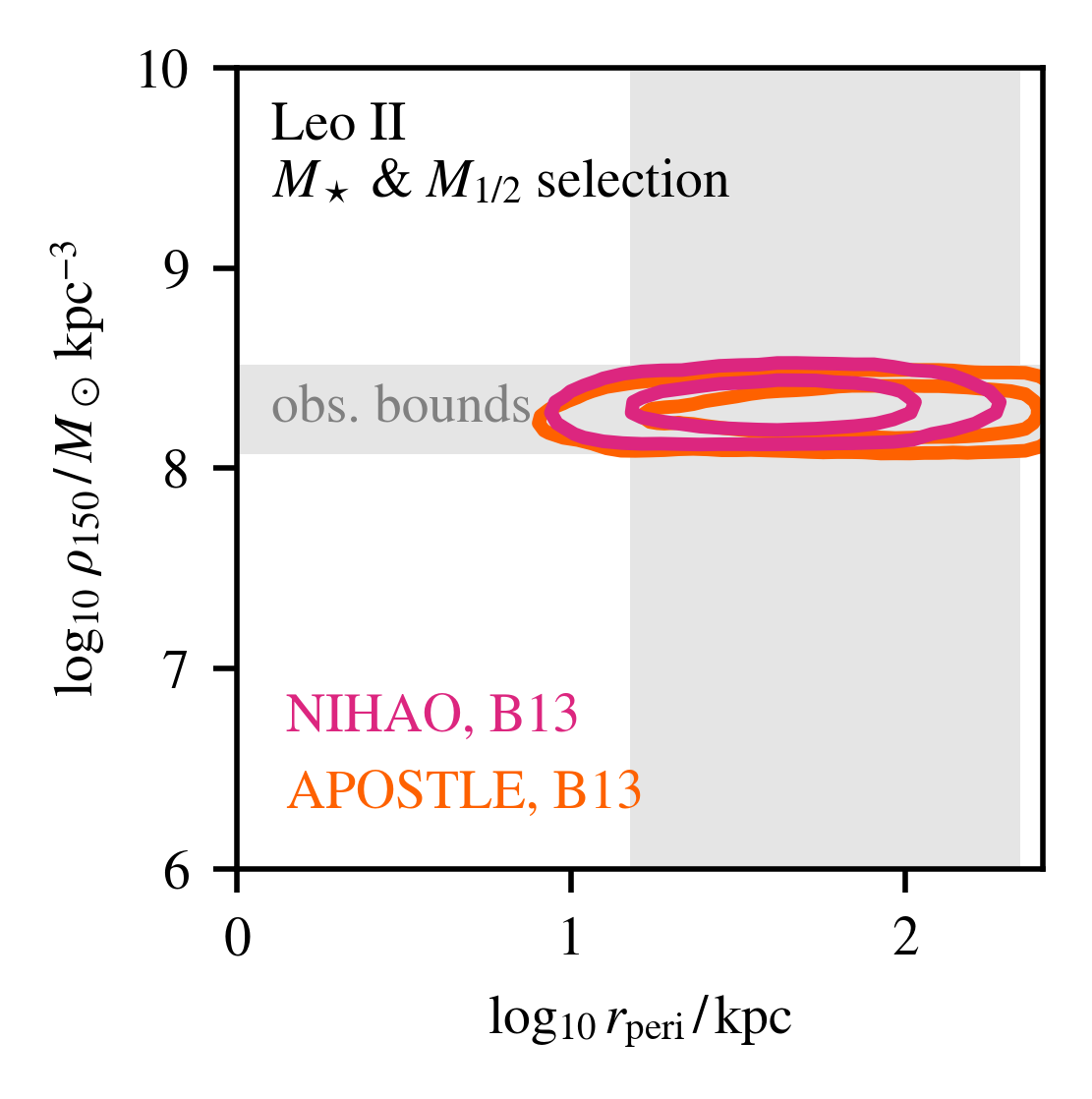
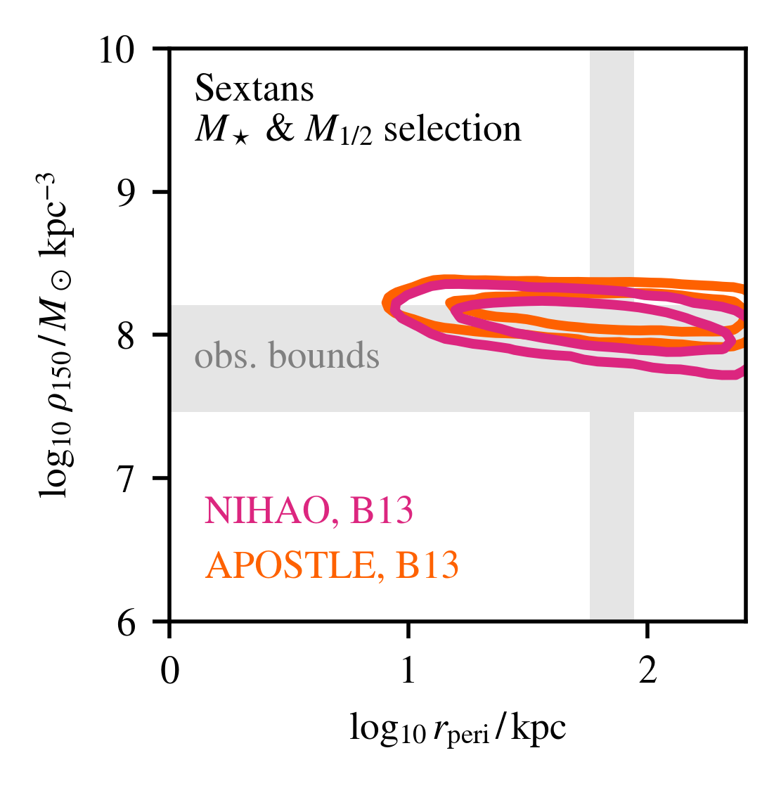
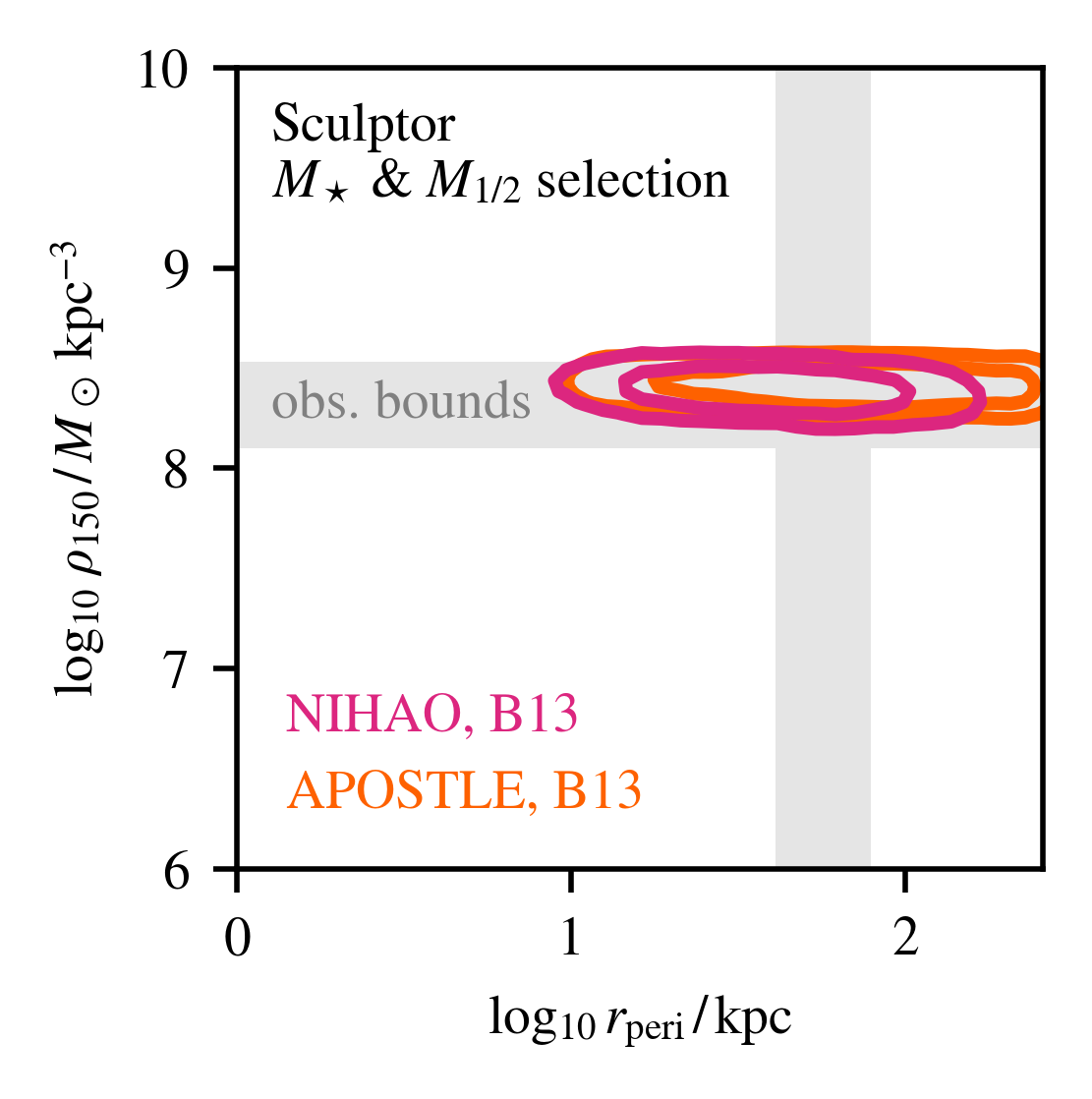
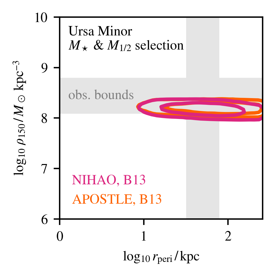
Figure 12: A version of Figure 4 for all classical satellites, using the B13 SMHM relation. Despite placing larger galaxies into smaller halos, the results are quite similar to the RP17 model shown above in Figure 11.

Figure 4 shows 68% and 95% containment regions for $f_{\,i}(\mathbf{x}{})$ in the 2D $r_{\mathrm{peri}}$ – $\rho_{150}$ plane for Fornax and Draco (in the language used in Section 2.2, $\mathbf{x}=(r_{\mathrm{peri}},\,\rho_{150}$)). This figure shows results for both feedback models and for the RP17 SMHM relation. In principle, one could use $\boldsymbol{\theta}=(M_{\star},\,M_{1/2},\,t_{\mathrm{infall}})$, however we find that $t_{\mathrm{infall}}$ is too poorly observationally constrained to provide meaningful information and thus choose $\boldsymbol{\theta}=(M_{\star},\,M_{1/2})$. The contours are compared to measurements from Fritz et al. (2018), Battaglia et al. (2022), and Pace et al. (2022) for $r_{\mathrm{peri}}$; and Read et al. (2019), Kaplinghat et al. (2019), and Hayashi et al. (2020) for $\rho_{150}$, shown as grey bands in the figure. The width of each of the grey bands corresponds to the maximum and minimum values consistent with observations to within $1\sigma$, marginalizing over all measurements including the choice of cusp or core in $\rho_{150}$ modeling or the choice of potential in modeling the pericenter (note that two of the $r_{\mathrm{peri}}$ models include an LMC-like partner with the MW potential, and this has a strong influence on the satellites’ orbits). Results for all classical satellites are presented in Figure 11 and equivalent plots using the B13 SMHM relation are presented in Figure 12.

Figure 4 reveals that the NIHAO feedback emulator cores Fornax-like dwarfs enough to shift the central density by nearly an order of magnitude relative to the APOSTLE feedback emulator. Correspondingly, the pericenter distribution of the Fornax-like satellites in the NIHAO emulator is shifted toward larger values than APOSTLE, suggesting that only extremely significant DM mass loss (with large initial masses) can lead to APOSTLE satellites simultaneously matching the observed $M_{\star}$ and $M_{1/2}$ values. This in particular provides a sharp insight into the interplay of feedback and orbital evolution: while the NIHAO feedback emulator forms Fornax-like satellites through coring, the APOSTLE model forms them through tidally stripping large-$M_{\star}$ galaxies until their $M_{1/2}$ is sufficiently low, which is a leading factor in Fornax analogues being so rare in the APOSTLE emulator (the APOSTLE contours for Fornax are dashed because of low statistics, cf. Table 2). Due to the unique status of Fornax’s mass parameters, feedback differences are most pronounced in this system; the distributions for analogues of the smaller dwarfs (Figure 11 and Figure 12) generally do not exhibit as strong a change, although some satellites present the same anticorrelation between the inferred pericenter and central density in both feedback models.

While the inferences made on the classical dwarfs’ density profiles (Section 3) are broadly consistent with observational models, the inference of Fornax’s central density and pericenter in particular provide constraining information on the semi-analytic models examined here. Due to the discrepancy shown in Figure 4, it seems that the APOSTLE feedback emulator struggles to simultaneously explain the combined observations of Fornax’s $\rho_{150}$, $r_{\mathrm{peri}}$, $M_{\star}$, and $M_{1/2}$. Such a multidimensional combined analysis is difficult to perform without semi-analytic techniques that allow for efficient scanning over the many sources of uncertainty present in galaxy formation. The semi-analytic technique reveals how rare it is to produce a dwarf such as Fornax.

4.2 Comparison of Accretion Modes

Lastly, we use SatGen to examine the likelihood that each of the classical satellites were directly accreted onto the MW, as opposed to entering as part of a larger group. SatGen resolves substructure due to hierarchical formation of the infalling satellite groups, and during orbital evolution, a satellite group can release some of its substructure into the MW. This release has a chance to occur whenever substructure passes outside the virial radius of its parent, with probability inversely proportional to the local dynamical time of the parent. Intuitively, the dynamical time at the location of the parent is the timescale on which the parent is tidally stripped; release of higher-order substructure is akin to tidal stripping.

It should be noted that SatGen does not account for all the orbital physics that a full simulation does. In particular, satellites orbit under the influence of their immediate parent object, but there is no prescription for, e.g., the reflex motion of the satellite system due to large infalling objects. Further, satellites of the same host have no direct gravitational influence on each other. Both of these behaviors are known to exist in simulations of MW analogs with large infalling systems like the LMC and can have detectable effects on the satellite population—see, e.g., Vasiliev (2023) and references therein. Furthermore, since satellites only orbit under their parent’s potential, any sub-substructure would not feel the potential of the MW, only that of its immediate parent. With these limitations in mind, one may still draw conclusions about the probability of a structure being bound to some larger system at the time of its infall and how these two modes of accretion might impact the resulting infall time, mass loss rates, pericenters, and other parameters.

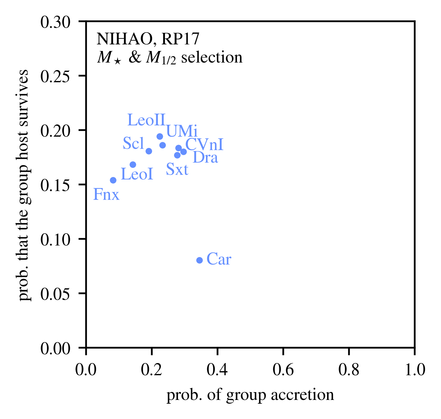
Figure 5: The probability that any given classical satellite is accreted as part of a group rather than directly from the field (as inferred though the $\boldsymbol{\theta}=(M_{\star},\,M_{1/2})$ selection). The vertical axis shows the probability that, given a group-accretion scenario, the original group host persists as a satellite of the MW. While the dwarfs presented here are unlikely to have been substructure at infall, in the case that they were, it is unlikely that the group host survived to the present day.

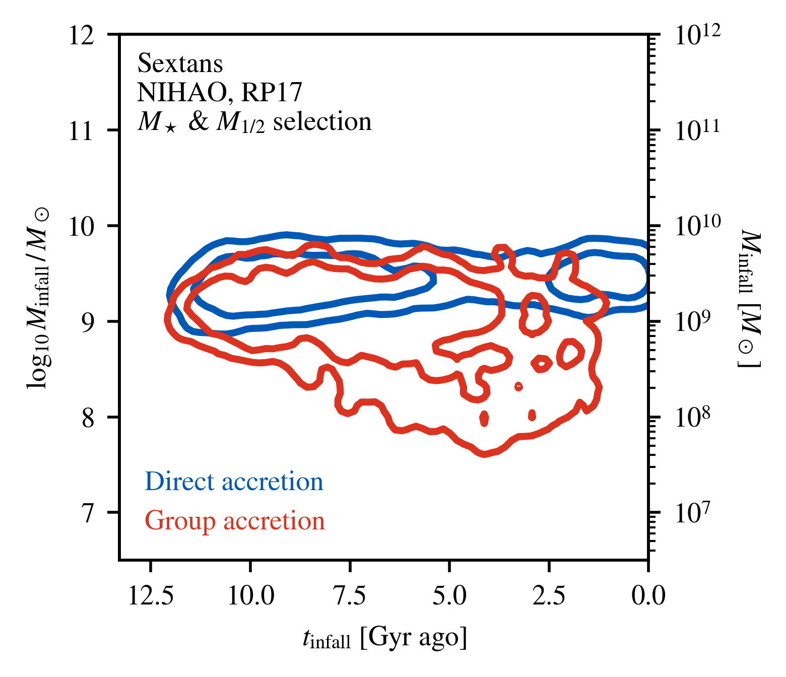
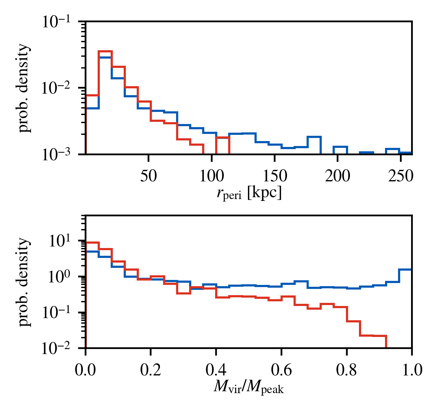
Figure 6: A demonstration of how a satellite galaxy’s properties depend on whether it is accreted directly onto the MW, shown in blue, or as part of a larger group, shown in red. (Left:) The inferred infall time and virial mass at infall as derived from directly- and group-accreted satellites based on their $M_{\star}$ and $M_{1/2}$, where the infall time is calculated as the time since the satellite (or the satellite group) crossed the virial radius of the MW. The directly-accreted satellites show a bimodality in this parameter space, which can be understood due to the population of splashback galaxies (see Figure 7 and discussion in the text). (Right:) The one-dimensional inferred probability distributions for $r_{\mathrm{peri}}$ (in the upper panel) and $M_{\mathrm{vir}}/M_{\mathrm{peak}}$ (in the lower panel). Satellites accreted as part of a group generally have lower pericenters and greater mass loss than directly-accreted satellites, a trend enhanced by the fact that there are no recently-accreted halos in this population; for directly-accreted satellites that have yet to complete a full orbit, their closest approach to the MW is recorded as their pericenter, and these do not lose much mass to tidal stripping. The mass loss that takes place in the group, prior to MW infall, is evident in the left panel; the group-accretion contour extends to lower masses than the direct-accretion contour. These trends are clear in Sextans, so it is used as an example, though Figure 13 contains corresponding plots for each of the other classical satellites.

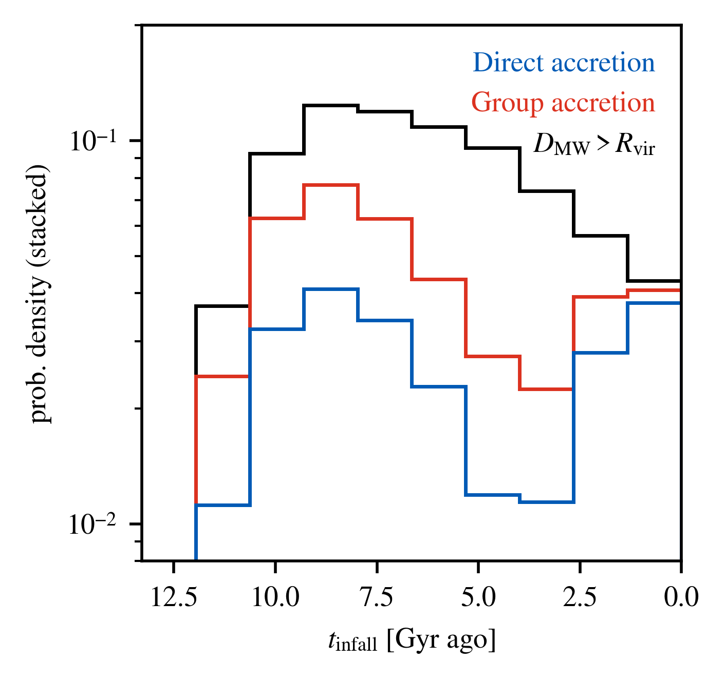
Figure 7: The stacked distribution of infall times of all surviving satellites, split into three components. Of the satellites that pass the cuts enumerated in Section 2.1, those that are directly accreted are shown in blue, while those accreted as part of a group are shown in red. Atop these is the set of “splashback galaxies,” i.e. satellites that are located at a distance from the MW, $D_{\mathrm{MW}}$, that is beyond its virial radius, $R_{\mathrm{vir}}$. Many satellites that fell in $\gtrsim 3$ Gyr ago are currently approaching their apocenters and may be instantaneously outside the virial radius of the MW at the present day. The requirement that $D_{\mathrm{MW}}\leq R_{\mathrm{vir}}$ therefore removes these splashback galaxies from our sample, leading to an apparent bimodality in the infall times of the surviving satellites in Figure 6.

A comparison of the chances of various accretion modes is shown in Figure 5—the abscissa shows the probability that a satellite is accreted with a group (as opposed to being accreted directly from the field), and the ordinate axis shows the probability that the group host survives to the present day in the case that the satellite has a parent. The satellites are selected to match the properties of the classical MW dwarfs using the $\boldsymbol{\theta}=(M_{\star},\,M_{1/2})$ inference. The SatGen analysis suggests that the classical satellites overwhelmingly form in the field, with a $23\%$ chance, on average, of entering the MW within a larger substructure. In general, SatGen predicts that satellites that match the classical dwarfs in $M_{\star}$ and $M_{1/2}$ and come in with a group only have a 16% chance of the group surviving, corresponding to an overall 4% absolute chance of having a surviving group host.

Group-accretion events are known to have an impact on the resulting satellite distribution, both in terms of the count of satellites and in their spatial distribution (Smercina et al., 2022; D’Souza & Bell, 2021). Figure 6 illustrates how the properties of the SatGen satellites vary depending on their origin. For example, the top right panel shows the inferred distance of closest approach of each satellite to the MW’s center (denoted $r_{\mathrm{peri}}$, but see caveat below), both for satellites accreted directly (blue) and for those accreted as part of a larger group (red). The bottom right panel shows the inferred mass loss in terms of the satellite’s present-day virial mass, $M_{\mathrm{vir}}$, relative to its peak mass, $M_{\mathrm{peak}}$. The latter is defined when the satellite exits the field and is accreted onto the host—either the MW, in the case of direct accretion, or the group host, in the case of group accretion.

As shown in the top right panel of Figure 6, the pericenter distribution peaks at roughly the same value for both the direct and group-accretion cases, however the former has an extended tail towards larger $r_{\mathrm{peri}}$. This is also observed as an extended tail at large $M_{\mathrm{vir}}/M_{\mathrm{peak}}$ in the bottom right panel of the figure. The extended tails in the direct-accretion satellites arise from the fact that these satellites are considered first-order as soon as they cross within the MW’s virial radius and are thus always included in our sample. In contrast, for the group-accretion scenario, the group host is the first-order satellite at infall, while objects bound to it are considered higher-order satellites of the MW. This higher-order structure must be released from the group to be included in the satellite sample considered here. As a result of this distinction, there is a population of recently accreted satellites that is present in the direct-infall population but not in the group-infall population. These satellites have little mass loss and have not completed a pericentric passage by $z=0$. Their location at $z=0$ is then their closest approach to the MW, but it is not truly their orbital pericenter. On the other hand, since groups tend to shed their satellites most efficiently near their own pericenters, the satellites contributed by such groups typically have experienced much closer approaches. In the lower panel, the mass loss of group-accreted satellites is enhanced, since they will undergo tidal stripping even before reaching the MW. Even when restricting the direct-infall population to those that have completed at least one pericentric passage, the group-accretion case prefers more recent infall times, smaller pericenters, and greater mass loss.

As a further exploration of the tidal mass loss, the left panel of Figure 6 shows the infall time into the MW, $t_{\mathrm{infall}}$, and the inferred mass at this time, $M_{\mathrm{infall}}$, for the two satellite populations. Due to the time spent evolving in the potential of their host, group-accretion satellites have a lower $M_{\mathrm{infall}}$ than those that are directly accreted, an effect exacerbated for satellites with more recent $t_{\mathrm{infall}}$ that evolved for longer within the group. The time of infall itself is also affected by the orbital dynamics of the accreting group. At very recent infall times, accretion is dominated by directly-accreting first-order satellites, since any infalling groups have not yet been stripped enough to release substructure into the MW. At slightly larger infall times there is a lull in the direct accretion, which corresponds to satellites that are at or near the apocenter of their orbit (e.g., Ludlow et al., 2009; Yun et al., 2019; Bakels et al., 2021; Engler et al., 2021). While dynamical friction efficiently pulls the groups toward low pericenters, directly-accreted satellites can maintain higher orbital energies and even exit the virial radius, becoming “splashback” satellites. Because we select only satellites with present-day distance $D_{\mathrm{MW}}$ within the MW’s virial radius $R_{\mathrm{vir}}$, splashback satellites are removed from our sample. Figure 7 demonstrates this explicitly, by plotting the distribution of infall times for both direct and group-accretion satellites, as well as the splashback satellites with $D_{\mathrm{MW}}>R_{\mathrm{vir}}$. The bimodality of $t_{\mathrm{infall}}$ is clear in the blue direct-accretion distribution, but adding in the population of splashback galaxies (black) fills in the gap between the two infall times. For completeness, the group-accreted satellites are also included in the probability distribution (red), since these three populations together comprise the entire set of surviving satellites.

While this study considers group accretion in general, these results may also be applied to the specific case of LMC-like groups. The LMC has a mass $\gtrsim 10^{11}~{}M_{\odot}$ (Vasiliev, 2023), so an interesting comparison is to restrict attention to accretion events in which the group host survives to $z=0$ with a mass $M_{\mathrm{vir}}\geq 10^{11}~{}M_{\odot}$. This happens in $\sim 10\%$ of the MW systems, although an additional $\sim 1.6$% have such an LMC-like group which has exited the MW’s virial radius. We find that the classical dwarfs in SatGen have a $\sim 0.5\%$ probability of originating from a surviving LMC host, consistent with orbital studies of these dwarfs (Sales et al., 2011; Erkal & Belokurov, 2020; Patel et al., 2020; Correa Magnus & Vasiliev, 2022; Battaglia et al., 2022; Pace et al., 2022). Restricting the analysis to LMC-like group accretion typically prefers $t_{\mathrm{infall}}\lesssim 4$ Gyr ago, since such large host halos take time to assemble and therefore would not be present in the early universe. In accordance with the lower inferred $t_{\mathrm{infall}}$, the pericenters are shifted to larger distances, although the inferred $r_{\mathrm{peri}}$ in the LMC case are often higher than other group-accretion scenarios with the same $t_{\mathrm{infall}}$, and they are also inferred to be closer to their $M_{\mathrm{peak}}$ than in the general group-accretion case. However, these trends should be understood with the warning that LMC infall events are rare and thus statistics-limited.

5 Conclusions

This work presents a novel method for inferring properties of MW dwarf galaxies using semi-analytic models of satellite systems. The foundation of the approach is a statistical sample of MW satellites generated using the semi-analytic model SatGen. This large sample, which almost completely captures cosmological halo-to-halo variance, can be produced quickly with SatGen, in contrast to $N$-body or hydrodynamical codes. One can then select in a principled way the satellites that have properties matching well-constrained observational parameters of MW dwarfs, such as their stellar mass $M_{\star}$ or total mass $M_{1/2}$ within the half-light radius. The distribution of selected SatGen satellites constitutes an inference for unknown properties of the MW dwarf itself.

We applied this method to three sets of inferences for the nine bright “classical dwarfs” of the MW. In particular, the procedure was used to:

1. infer the structural parameters $(r_{\text{max}},\,v_{\text{max}})$ describing the DM halos of the dwarfs, accounting for systematic uncertainties present in this inference due to the SMHM relation and feedback modeling. The results of this study, which are compiled in Table 3, generally agree with Jeans analyses and predictions from empirical scaling relations, but include a more comprehensive modeling of systematic uncertainties and a realistic, correlated uncertainty band on the inferred halo parameters.

2. infer the correlations between orbital parameters of a dwarf galaxy and its internal properties. Importantly, we showed that the correlation between a galaxy’s central density and pericenter provides a means to constrain uncertainties in the feedback modeling. For example, the only satellites that simultaneously matched the observed $M_{\star}$ and $M_{1/2}$ of Fornax in the APOSTLE feedback emulator (which prefers cuspier halos) had lower pericenter and higher central density than expected from observations. On the other hand, the NIHAO feedback emulator, which cores satellite galaxies more efficiently, yielded a population of high-$M_{\star}$, low-$M_{1/2}$ galaxies in much better agreement with the observed parameters for Fornax. This preference for the stronger feedback model is evinced not only by the agreement of the central densities but also in the statistical prevalence: there are very few satellites in the APOSTLE emulator sample that accurately reproduce both the $M_{\star}$ and $M_{1/2}$ of Fornax, but the NIHAO emulator produces many more, by two orders of magnitude.

3. infer the likelihood that a given dwarf is associated with the LMC or other larger structure at the time of its accretion, and to infer the differences between this case and the case of direct accretion from the field. Based solely on the present-day $M_{\star}$ and $M_{1/2}$ of the classical satellites, we found no convincing evidence that any were associated with larger systems, in agreement with detailed orbital modeling studies. In the event that they were, the inferred properties are more consistent with smaller pericenters and greater mass loss.

In each of the above scenarios, the space of MW satellites was constrained using only observations of $M_{\star}$ and $M_{1/2}$ and found to be in good agreement with analyses that leveraged more difficult observations of internal kinematics or systemic motions. Despite the successes of the method, it is important to recognize assumptions that have been made to enable efficient computation. While SatGen is well-calibrated to reproduce results from idealized and cosmological simulations, it still relies on a number of simplifying assumptions and empirical fits. For example, satellites orbit only under the influence of their immediate parent; satellites of the same host have no impact on each other; and there is no prescription for the reflex motion of the parent due to LMC-like satellites. Further, DM potentials are modeled as perfectly spherical and follow a particular functional form, with the only non-spherical component being the MW disk.

As our understanding of galaxy formation grows, semi-analytic models will continue to improve in accuracy and complexity, allowing for sharper analyses across a broader domain of parameters. One particularly promising direction is the use of semi-analytic satellite generators to constrain feedback prescriptions. As our results demonstrate, correlations between orbital parameters and internal properties of a dwarf galaxy can be used to distinguish between different feedback emulators (specifically, NIHAO and APOSTLE). An even more powerful and generic approach would be to parameterize the feedback model within SatGen, and to then directly constrain the feedback parameters on data using a full likelihood analysis. With analytic models for gas ejection (e.g. Li et al., 2023), SatGen could have a more physically-motivated parameterization for the response of the DM halo to gas ejection, rather than simply changing the inner slope and concentration. Such developments are on the horizon for semi-analytic models like SatGen, and will allow for even more robust study of baryonic feedback and the galaxy–halo connection.

Data Availability

The data underlying this article are available via Zenodo at https://zenodo.org/doi/10.5281/zenodo.10068111. The code used to perform the inferences in this work is publicly available in the GitHub repository https://github.com/folsomde/Semianalytic_Inference.

Appendix A Supplementary figures

In the main body of this paper, specific dwarfs are highlighted in the figures. For completeness, the figures below include versions of Figure 3, Figure 4, and Figure 6 for all nine bright MW spheroidal dwarfs. For more detail regarding the data shown in these figures, see the captions provided for the figures in the main text. Figure 9 has no corresponding figure in the main text; it shows the inferred inner slopes in the NIHAO and APOSTLE feedback emulators assuming the RP17 SMHM relation and is referenced in Section 3.2. Figure 10 also has no corresponding figure in the main text; it shows the inferred virial mass at the time of accretion onto the MW and the $z=0$ stellar mass for all nine satellites in the NIHAO and APOSTLE feedback emulators assuming the RP17 SMHM relation and is referenced in Section 3.2.

Figure 8: A version of Figure 3 for all classical satellites.

NIHAO, RP17 APOSTLE, RP17 Simple scaling relations E18 cored   cuspy K19 cored   cuspy A23

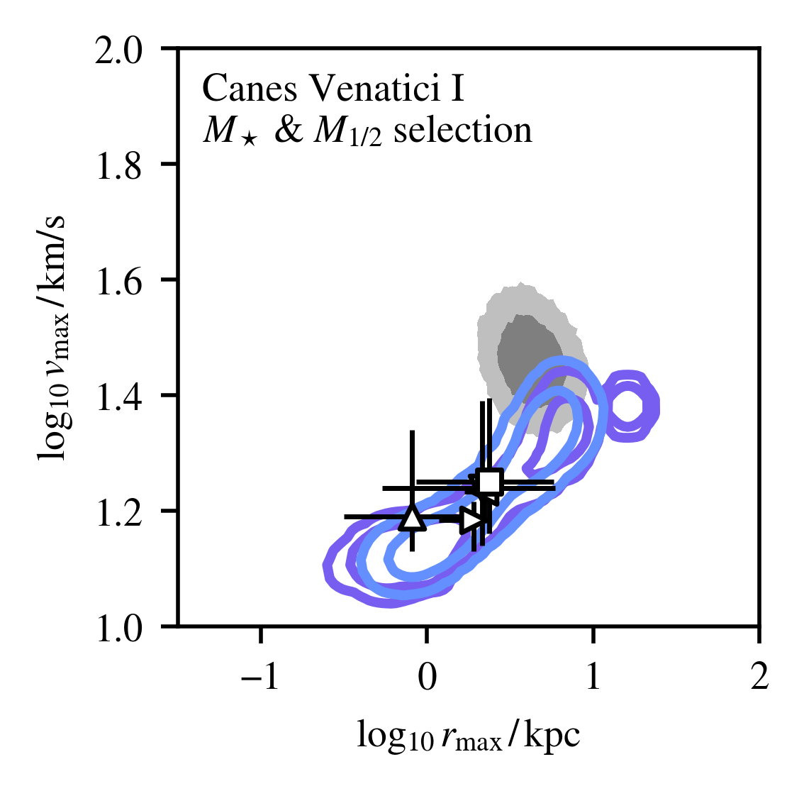
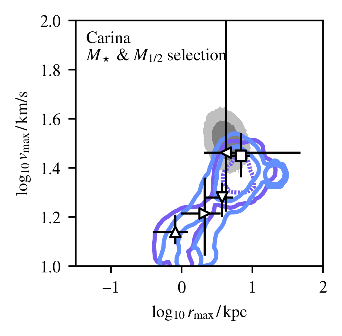
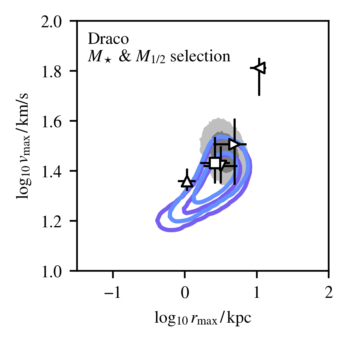
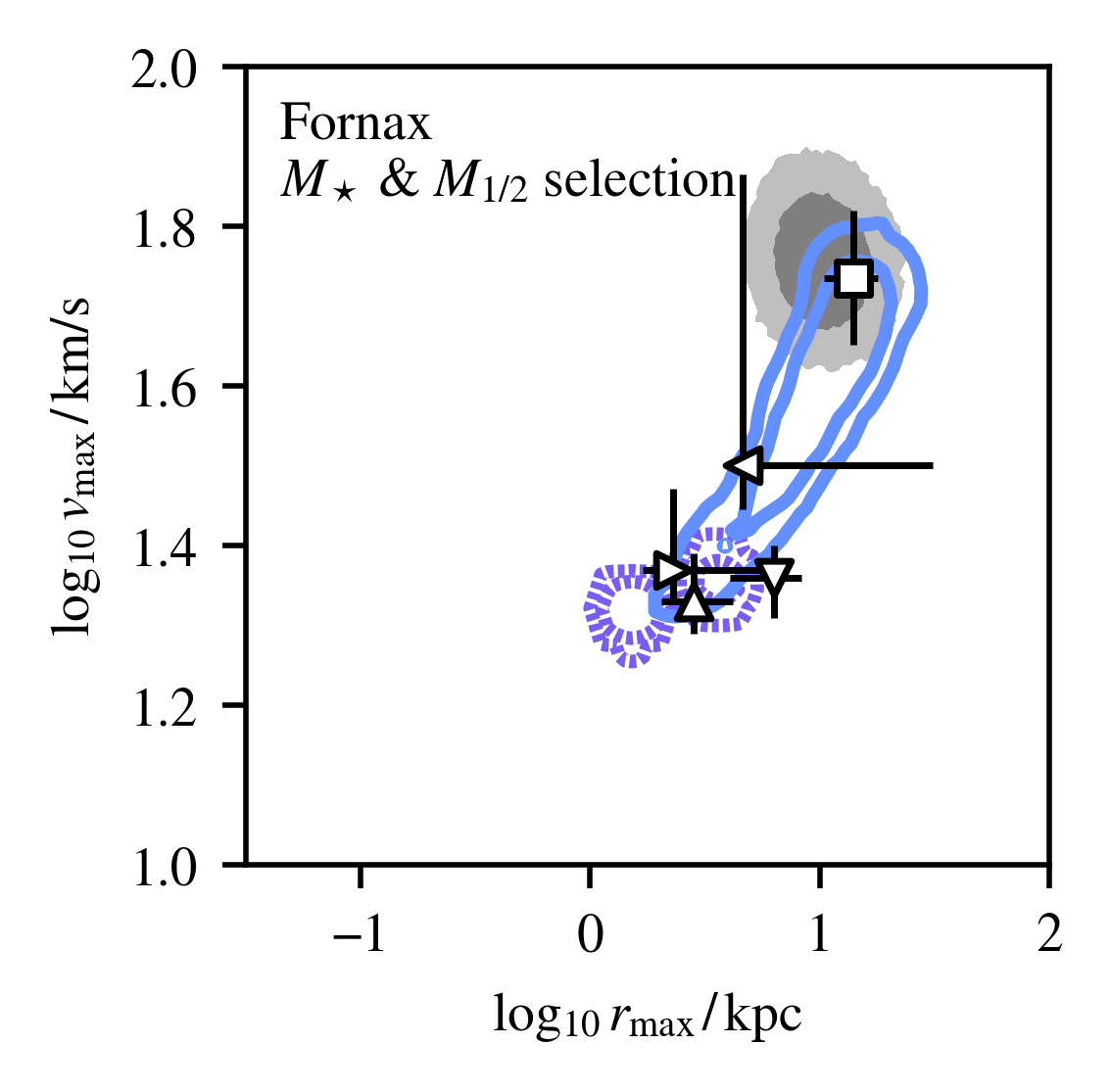
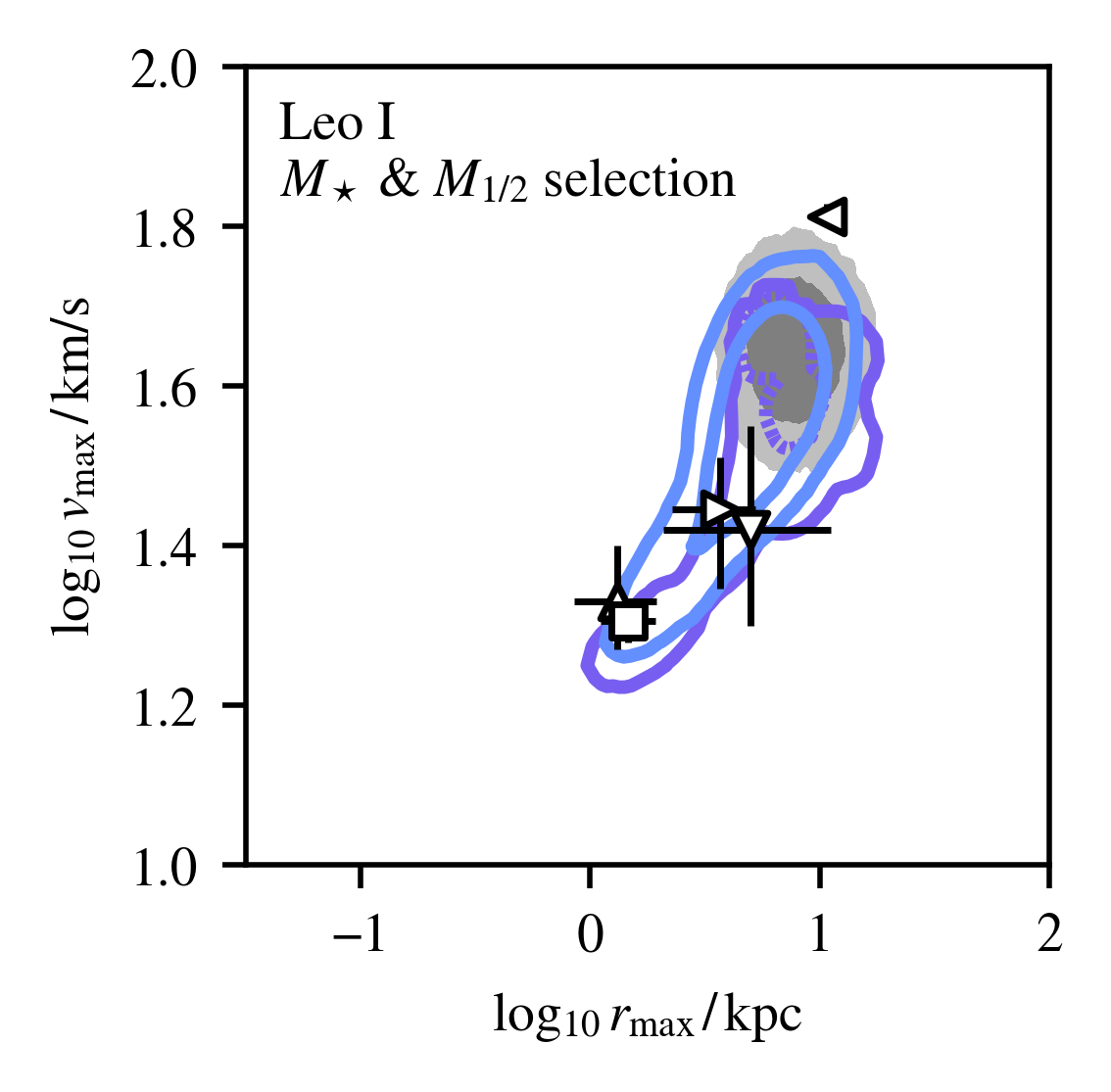
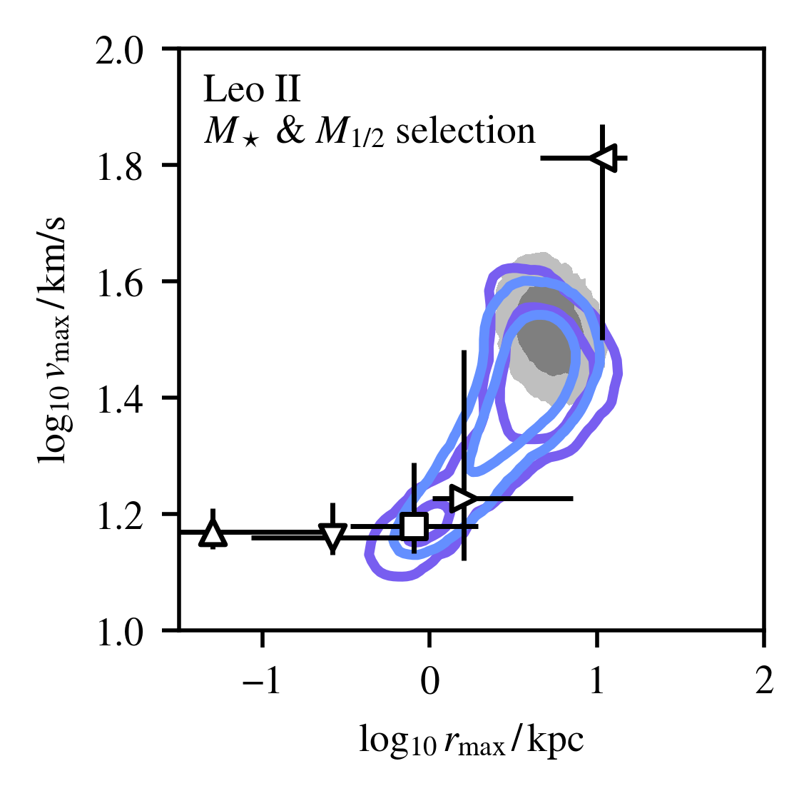
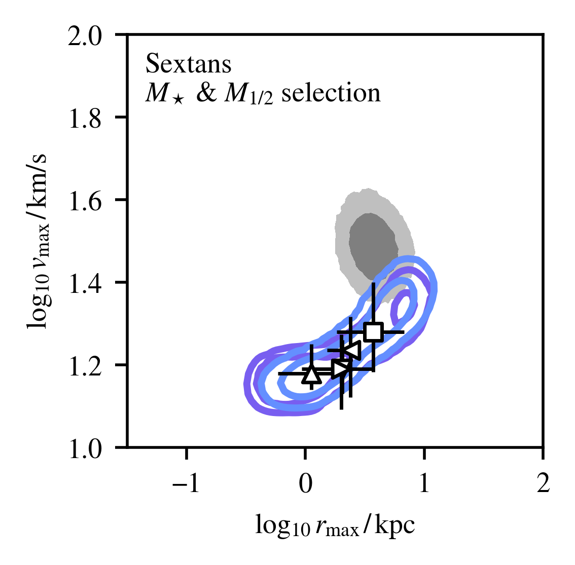
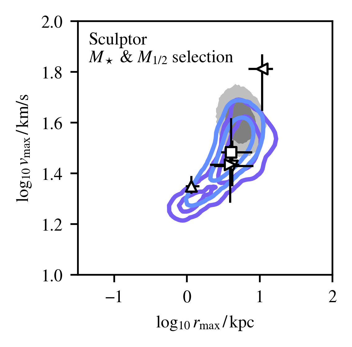
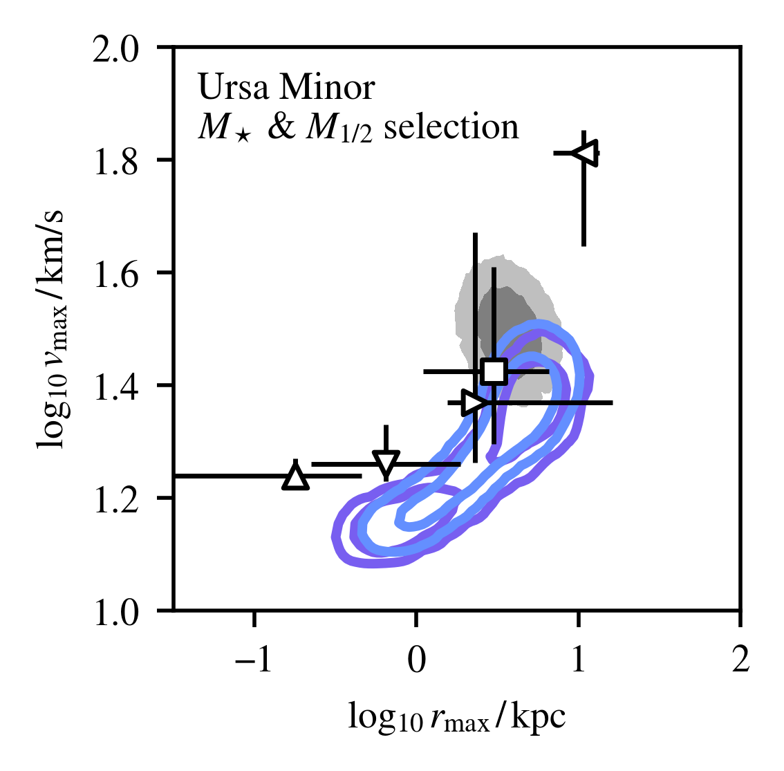
Figure 9: Inferred inner slopes for all classical satellites, assuming the RP17 SMHM relation and varying over feedback emulation. The slope is parameterized by $s_{0.01}$, which is the slope at $1\%$ of the virial radius. For an NFW profile, this will range from 1 to about 1.5 depending on the concentration, while particularly cored profiles will approach zero. The dashed lines show the median inferred slope, though the full distributions are shown for clarity. Fornax and Sextans are particularly interesting for the large difference between feedback models.

NIHAO, RP17  APOSTLE, RP17

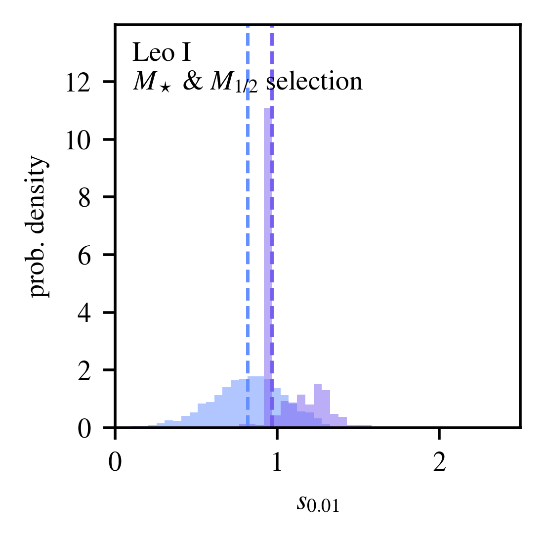
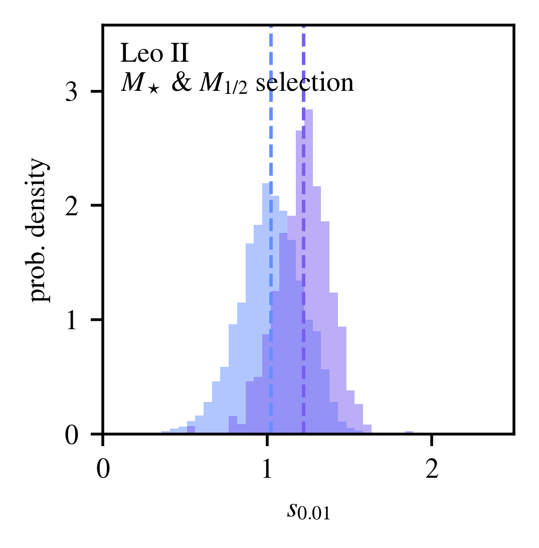
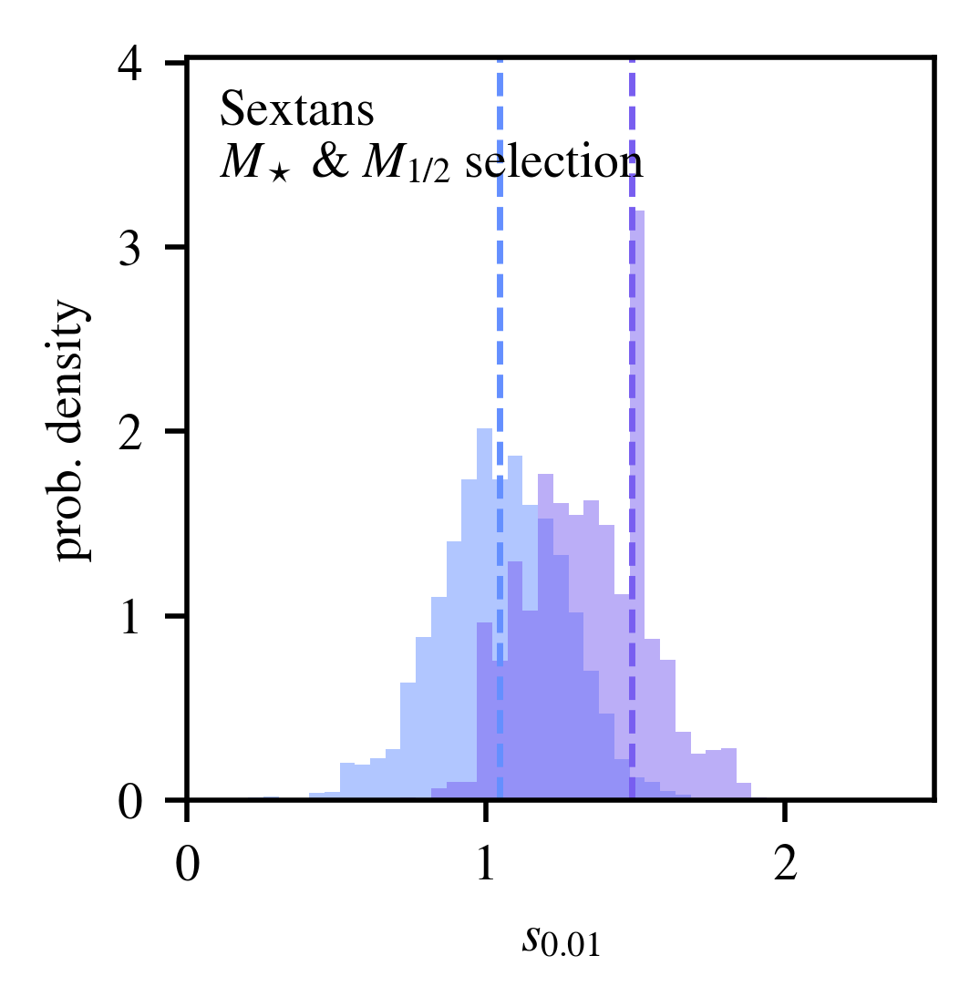
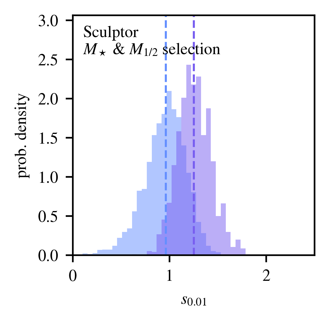
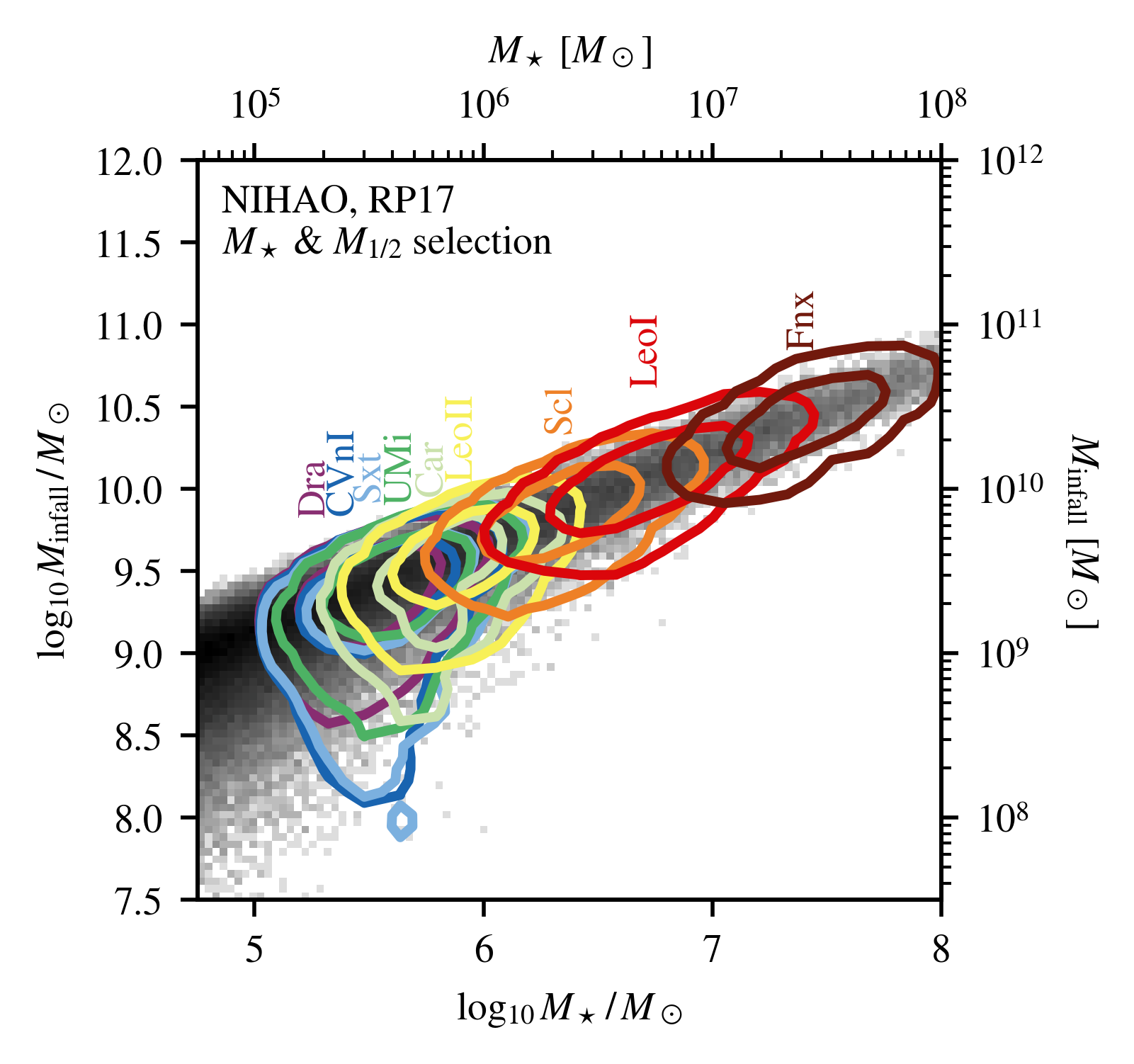
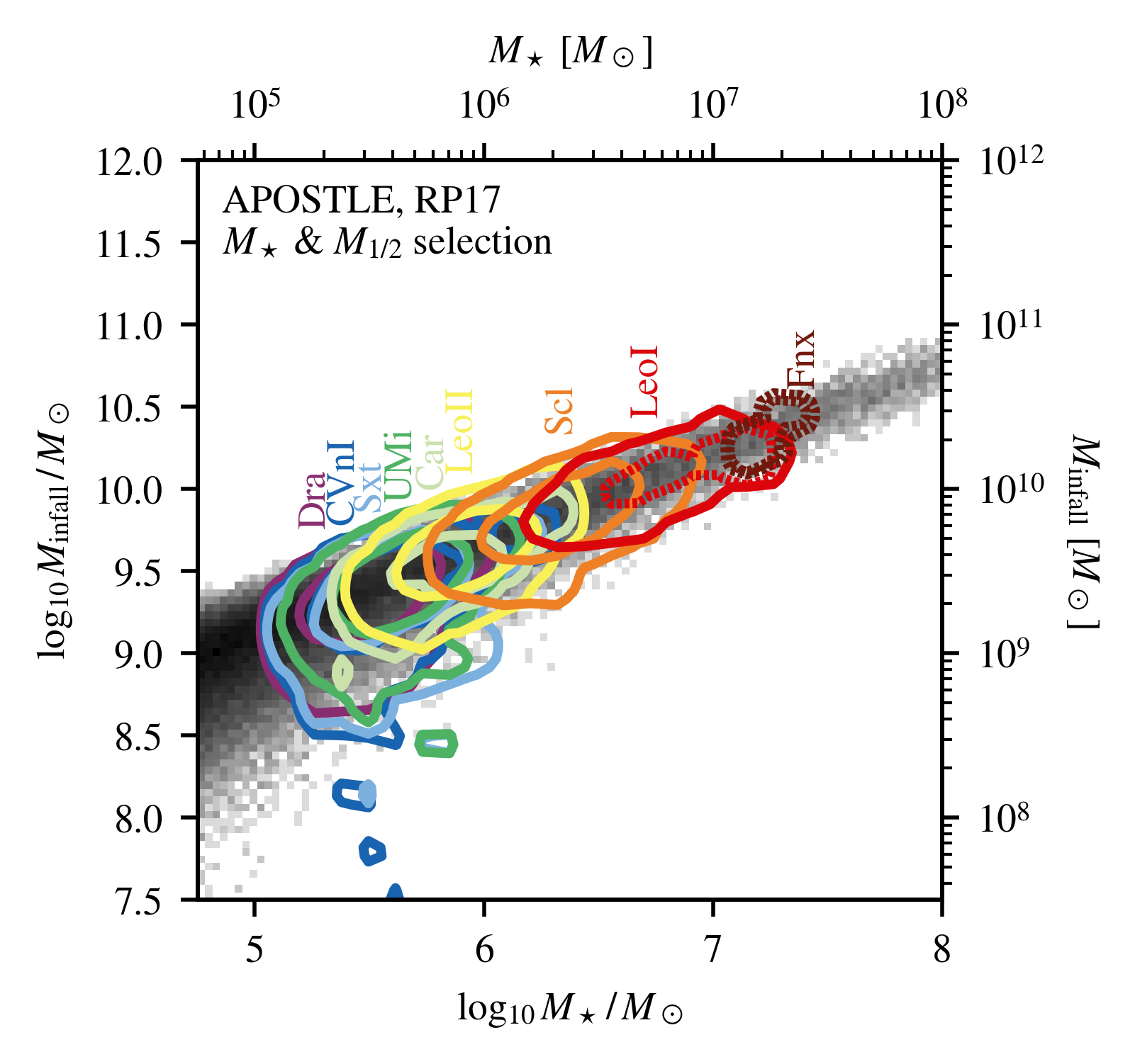
Figure 10: 68 and 95% confidence intervals for the $z=0$ stellar mass, $M_{\star}$, and the virial mass at the time of accretion into the MW, $M_{\mathrm{infall}}$, for each of the nine bright spheroidal dwarfs using the combined $M_{\star}$ and $M_{1/2}$-based inference. The gray histogram shows the overall distribution of SatGen satellites in the NIHAO feedback emulator (left) and in the APOSTLE feedback emulator (right). This is in large part set by the SMHM relation, though (i) $M_{\mathrm{infall}}$ is modified from the SMHM relation in satellites accreted as part of a group system, as they undergo tidal mass loss prior to infall, and (ii) $M_{\star}$ evolves along the Errani et al. (2018) tidal tracks, which prescribes the stellar mass lost in halos with significant DM mass loss.

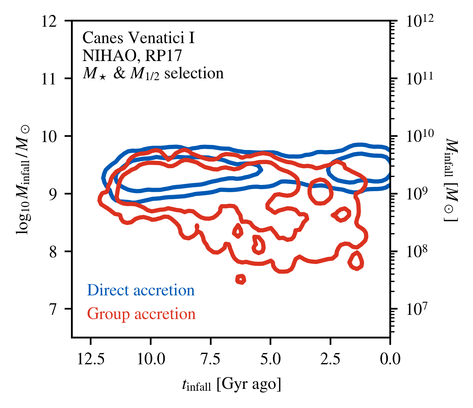
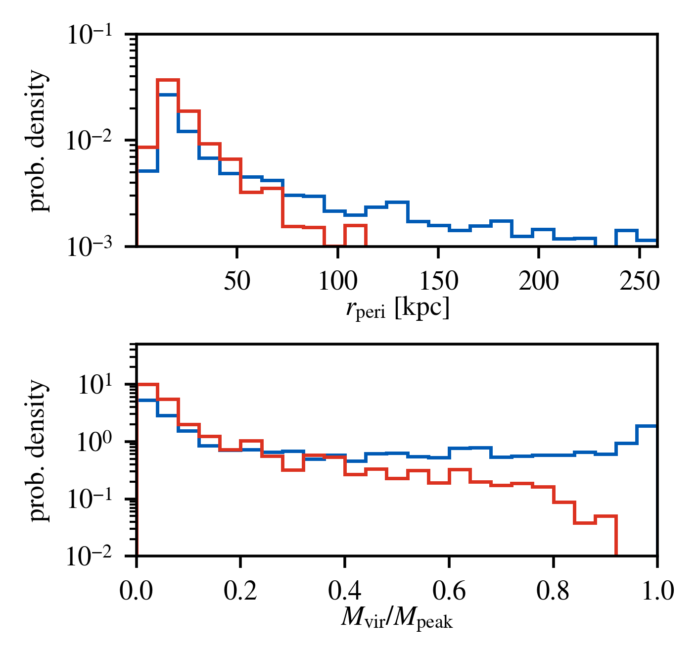
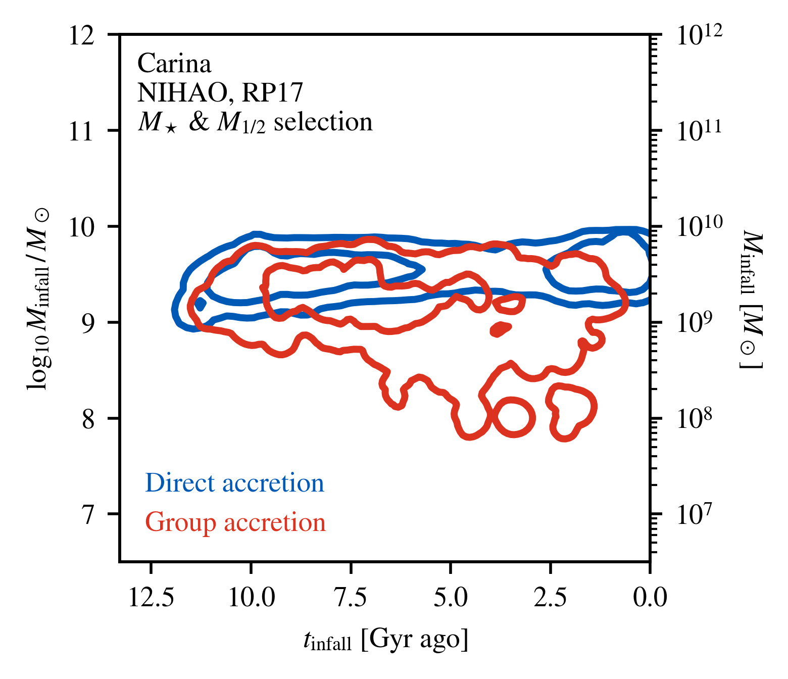
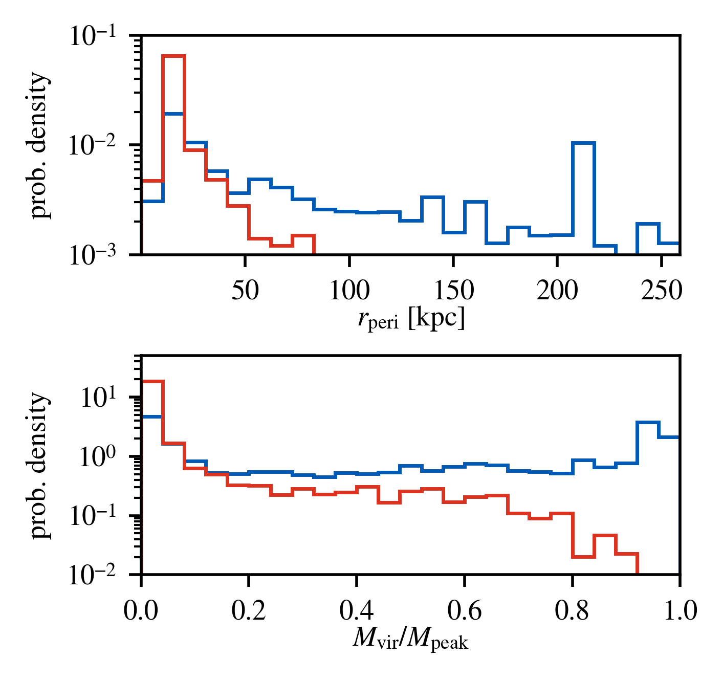
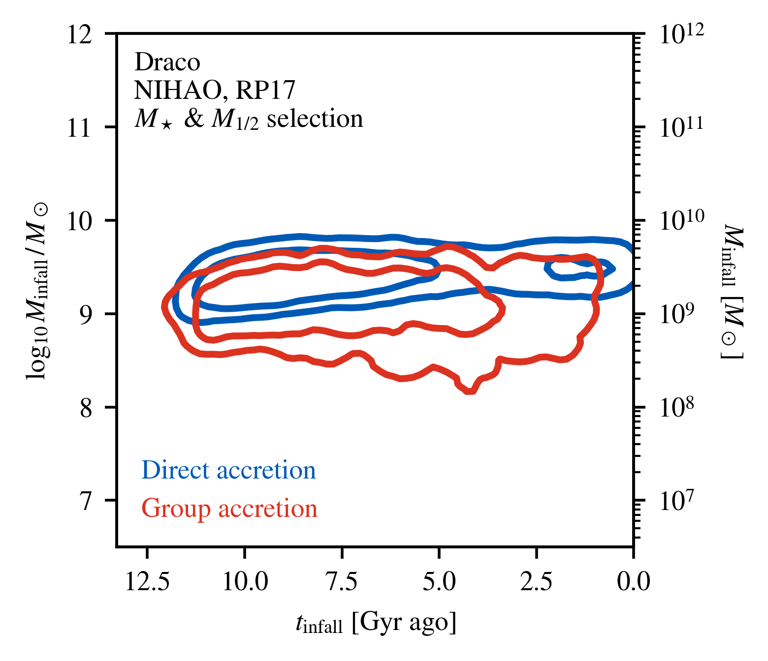
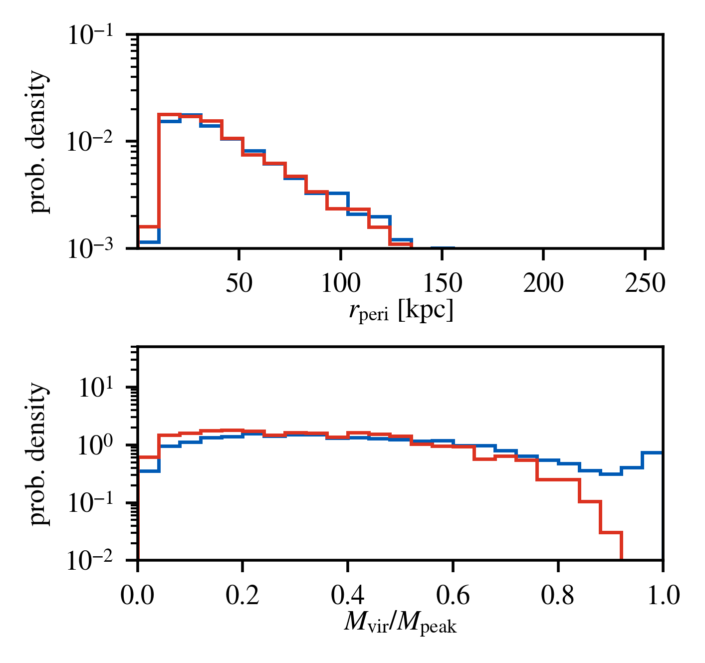
Figure 13: A version of Figure 6 for all classical satellites.

References

- Ando et al. (2020) Ando S., Geringer-Sameth A., Hiroshima N., Hoof S., Trotta R., Walker M. G., 2020, Physical Review D, 102, 061302
- Andrade et al. (2023) Andrade K. E., Kaplinghat M., Valli M., 2023, preprint, doi:10.48550/arXiv.2311.01528
- Astropy Collaboration et al. (2022) Astropy Collaboration et al., 2022, ApJ, 935, 167
- Bakels et al. (2021) Bakels L., Ludlow A. D., Power C., 2021, MNRAS, 501, 5948
- Barber et al. (2014) Barber C., Starkenburg E., Navarro J. F., McConnachie A. W., Fattahi A., 2014, MNRAS, 437, 959
- Battaglia et al. (2022) Battaglia G., Taibi S., Thomas G. F., Fritz T. K., 2022, A&A, 657, A54
- Behroozi et al. (2010) Behroozi P. S., Conroy C., Wechsler R. H., 2010, ApJ, 717, 379
- Behroozi et al. (2013) Behroozi P. S., Wechsler R. H., Conroy C., 2013, ApJ, 770, 57
- Behroozi et al. (2019) Behroozi P., Wechsler R. H., Hearin A. P., Conroy C., 2019, MNRAS, 488, 3143
- Bland-Hawthorn & Gerhard (2016) Bland-Hawthorn J., Gerhard O., 2016, ARA&A, 54, 529
- Boldrini et al. (2019) Boldrini P., Mohayaee R., Silk J., 2019, MNRAS, 485, 2546
- Brooks et al. (2013) Brooks A. M., Kuhlen M., Zolotov A., Hooper D., 2013, ApJ, 765, 22
- Chandrasekhar (1943) Chandrasekhar S., 1943, ApJ, 97, 255
- Cole et al. (2012) Cole D. R., Dehnen W., Read J. I., Wilkinson M. I., 2012, MNRAS, 426, 601
- Conroy et al. (2006) Conroy C., Wechsler R. H., Kravtsov A. V., 2006, ApJ, 647, 201
- Correa Magnus & Vasiliev (2022) Correa Magnus L., Vasiliev E., 2022, MNRAS, 511, 2610
- D’Souza & Bell (2021) D’Souza R., Bell E. F., 2021, MNRAS, 504, 5270
- Danieli et al. (2023) Danieli S., Greene J. E., Carlsten S., Jiang F., Beaton R., Goulding A. D., 2023, ApJ, 956, 6
- Dekel et al. (2017) Dekel A., Ishai G., Dutton A. A., Maccio A. V., 2017, MNRAS, 468, 1005
- Dekker et al. (2022) Dekker A., Ando S., Correa C. A., Ng K. C. Y., 2022, Physical Review D, 106, 123026
- Diemand et al. (2007) Diemand J., Kuhlen M., Madau P., 2007, ApJ, 667, 859
- Engler et al. (2021) Engler C., et al., 2021, MNRAS, 500, 3957
- Erkal & Belokurov (2020) Erkal D., Belokurov V. A., 2020, MNRAS, 495, 2554
- Errani et al. (2018) Errani R., Peñarrubia J., Walker M. G., 2018, MNRAS, 481, 5073
- Fillingham et al. (2019) Fillingham S. P., et al., 2019, preprint, doi:10.48550/arXiv.1906.04180
- Font et al. (2011) Font A. S., et al., 2011, MNRAS, 417, 1260
- Freundlich et al. (2020) Freundlich J., et al., 2020, MNRAS, 499, 2912
- Fritz et al. (2018) Fritz T. K., Battaglia G., Pawlowski M. S., Kallivayalil N., van der Marel R., Sohn S. T., Brook C., Besla G., 2018, A&A, 619, A103
- Garrison-Kimmel et al. (2017) Garrison-Kimmel S., et al., 2017, MNRAS, 471, 1709
- Genina et al. (2022) Genina A., Read J. I., Fattahi A., Frenk C. S., 2022, MNRAS, 510, 2186
- Gnedin et al. (2004) Gnedin O. Y., Kravtsov A. V., Klypin A. A., Nagai D., 2004, ApJ, 616, 16
- Green & van den Bosch (2019) Green S. B., van den Bosch F. C., 2019, MNRAS, 490, 2091
- Green et al. (2022) Green S. B., van den Bosch F. C., Jiang F., 2022, MNRAS, 509, 2624
- Guo et al. (2011) Guo Q., et al., 2011, MNRAS, 413, 101
- Guo et al. (2015) Guo Q., Cooper A. P., Frenk C., Helly J., Hellwing W. A., 2015, MNRAS, 454, 550
- Harris et al. (2020) Harris C. R., et al., 2020, Nature, 585, 357
- Hayashi et al. (2020) Hayashi K., Chiba M., Ishiyama T., 2020, ApJ, 904, 45
- Hiroshima et al. (2018) Hiroshima N., Ando S., Ishiyama T., 2018, Physical Review D, 97, 123002
- Hunter (2007) Hunter J. D., 2007, Comput. Sci. Eng., 9, 90
- Jardel & Gebhardt (2012) Jardel J. R., Gebhardt K., 2012, ApJ, 746, 89
- Jiang et al. (2019) Jiang F., et al., 2019, MNRAS, 488, 4801
- Jiang et al. (2021) Jiang F., Dekel A., Freundlich J., van den Bosch F. C., Green S. B., Hopkins P. F., Benson A., Du X., 2021, MNRAS, 502, 621
- Kaplinghat et al. (2019) Kaplinghat M., Valli M., Yu H.-B., 2019, MNRAS, 490, 231
- Kluyver et al. (2016) Kluyver T., et al., 2016, in Loizides F., Scmidt B., eds, Positioning and Power in Academic Publishing: Players, Agents and Agendas. IOS Press, pp 87–90, https://eprints.soton.ac.uk/403913/
- Koposov et al. (2009) Koposov S. E., Yoo J., Rix H.-W., Weinberg D. H., Macciò A. V., Escudé J. M., 2009, ApJ, 696, 2179
- Kowalczyk et al. (2019) Kowalczyk K., del Pino A., Łokas E. L., Valluri M., 2019, MNRAS, 482, 5241
- Kravtsov et al. (2004) Kravtsov A. V., Berlind A. A., Wechsler R. H., Klypin A. A., Gottlöber S., Allgood B., Primack J. R., 2004, ApJ, 609, 35
- Li et al. (2010) Li Y.-S., De Lucia G., Helmi A., 2010, MNRAS, 401, 2036
- Li et al. (2020) Li Z.-Z., Zhao D.-H., Jing Y. P., Han J., Dong F.-Y., 2020, ApJ, 905, 177
- Li et al. (2023) Li Z. Z., Dekel A., Mandelker N., Freundlich J., François T. L., 2023, MNRAS, 518, 5356
- Lu et al. (2016) Lu Y., Benson A., Mao Y.-Y., Tonnesen S., Peter A. H. G., Wetzel A. R., Boylan-Kolchin M., Wechsler R. H., 2016, ApJ, 830, 59
- Ludlow et al. (2009) Ludlow A. D., Navarro J. F., Springel V., Jenkins A., Frenk C. S., Helmi A., 2009, ApJ, 692, 931
- Macciò et al. (2010) Macciò A. V., Kang X., Fontanot F., Somerville R. S., Koposov S., Monaco P., 2010, MNRAS, 402, 1995
- Meadows et al. (2020) Meadows N., Navarro J. F., Santos-Santos I., Benítez-Llambay A., Frenk C., 2020, MNRAS, 491, 3336
- Miyamoto & Nagai (1975) Miyamoto M., Nagai R., 1975, PASJ, 27, 533
- Moliné et al. (2017) Moliné Á., Sánchez-Conde M. A., Palomares-Ruiz S., Prada F., 2017, MNRAS, 466, 4974
- Moliné et al. (2023) Moliné Á., et al., 2023, MNRAS, 518, 157
- Moster et al. (2013) Moster B. P., Naab T., White S. D. M., 2013, MNRAS, 428, 3121
- Muñoz et al. (2018) Muñoz R. R., Côté P., Santana F. A., Geha M., Simon J. D., Oyarzún G. A., Stetson P. B., Djorgovski S. G., 2018, ApJ, 860, 66
- Munshi et al. (2021) Munshi F., Brooks A. M., Applebaum E., Christensen C. R., Quinn T., Sligh S., 2021, ApJ, 923, 35
- Nadler et al. (2019) Nadler E. O., Mao Y.-Y., Green G. M., Wechsler R. H., 2019, ApJ, 873, 34
- Nadler et al. (2023) Nadler E. O., et al., 2023, ApJ, 945, 159
- Navarro et al. (1997) Navarro J. F., Frenk C. S., White S. D. M., 1997, ApJ, 490, 493
- Neto et al. (2007) Neto A. F., et al., 2007, MNRAS, 381, 1450
- Pace et al. (2022) Pace A. B., Erkal D., Li T. S., 2022, ApJ, 940, 136
- Parkinson et al. (2007) Parkinson H., Cole S., Helly J., 2007, MNRAS, 383, 557
- Patel et al. (2020) Patel E., et al., 2020, ApJ, 893, 121
- Pedregosa et al. (2011) Pedregosa F., et al., 2011, JMLR, 12, 2825
- Peñarrubia et al. (2009) Peñarrubia J., Navarro J. F., McConnachie A. W., Martin N. F., 2009, ApJ, 698, 222
- Peñarrubia et al. (2010) Peñarrubia J., Benson A. J., Walker M. G., Gilmore G., McConnachie A. W., Mayer L., 2010, MNRAS, 406, 1290
- Pérez & Granger (2007) Pérez F., Granger B. E., 2007, Comput. Sci. Eng., 9, 21
- Pullen et al. (2014) Pullen A. R., Benson A. J., Moustakas L. A., 2014, ApJ, 792, 24
- Read et al. (2019) Read J. I., Walker M. G., Steger P., 2019, MNRAS, 484, 1401
- Rodríguez-Puebla et al. (2017) Rodríguez-Puebla A., Primack J. R., Avila-Reese V., Faber S. M., 2017, MNRAS, 470, 651
- Sales et al. (2011) Sales L. V., Navarro J. F., Cooper A. P., White S. D. M., Frenk C. S., Helmi A., 2011, MNRAS, 418, 648
- Sanders & Evans (2016) Sanders J. L., Evans N. W., 2016, ApJ, 830, L26
- Sawala et al. (2016) Sawala T., et al., 2016, MNRAS, 457, 1931
- Smercina et al. (2022) Smercina A., Bell E. F., Samuel J., D’Souza R., 2022, ApJ, 930, 69
- Starkenburg et al. (2013) Starkenburg E., et al., 2013, MNRAS, 429, 725
- Taylor & Babul (2001) Taylor J. E., Babul A., 2001, ApJ, 559, 716
- Tollet et al. (2016) Tollet E., et al., 2016, MNRAS, 456, 3542
- Vasiliev (2023) Vasiliev E., 2023, Galaxies, 11, 59
- Virtanen et al. (2020) Virtanen P., et al., 2020, Nat. Methods, 17, 261
- Vogelsberger et al. (2020) Vogelsberger M., Marinacci F., Torrey P., Puchwein E., 2020, Nature Reviews Physics, 2, 42
- Wang et al. (2015) Wang L., Dutton A. A., Stinson G. S., Macciò A. V., Penzo C., Kang X., Keller B. W., Wadsley J., 2015, MNRAS, 454, 83
- Wang et al. (2020) Wang W., Han J., Cautun M., Li Z., Ishigaki M. N., 2020, Sci. Chin. Phys. Mech. Astron., 63, 109801
- Wechsler & Tinker (2018) Wechsler R. H., Tinker J. L., 2018, Annu. Rev. Astron. Astrophys., 56, 435
- Wolf et al. (2010) Wolf J., Martinez G. D., Bullock J. S., Kaplinghat M., Geha M., Muñoz R. R., Simon J. D., Avedo F. F., 2010, MNRAS, 406, 1220
- Woo et al. (2008) Woo J., Courteau S., Dekel A., 2008, MNRAS, 390, 1453
- Yun et al. (2019) Yun K., et al., 2019, MNRAS, 483, 1042
- Zhao (1996) Zhao H., 1996, MNRAS, 278, 488
- Zhao et al. (2009) Zhao D. H., Jing Y. P., Mo H. J., Börner G., 2009, ApJ, 707, 354
- van den Bosch & Ogiya (2018) van den Bosch F. C., Ogiya G., 2018, MNRAS, 475, 4066
- van den Bosch et al. (2018) van den Bosch F. C., Ogiya G., Hahn O., Burkert A., 2018, MNRAS, 474, 3043