First Detailed Calculation of Atmospheric Neutrino Foregrounds
to the Diffuse Supernova Neutrino Background in Super-Kamiokande

Abstract

The Diffuse Supernova Neutrino Background (DSNB) — a probe of the core-collapse mechanism and the cosmic star-formation history — has not been detected, but its discovery may be imminent. A significant obstacle for DSNB detection in Super-Kamiokande (Super-K) is detector backgrounds, especially due to atmospheric neutrinos (more precisely, these are foregrounds), which are not sufficiently understood. We perform the first detailed theoretical calculations of these foregrounds in the range 16–90 MeV in detected electron energy, taking into account several physical and detector effects, quantifying uncertainties, and comparing our predictions to the 15.9 livetime years of pre-gadolinium data from Super-K stages I–IV. We show that our modeling reasonably reproduces this low-energy data as well as the usual high-energy atmospheric-neutrino data. To accelerate progress on detecting the DSNB, we outline key actions to be taken in future theoretical and experimental work. In a forthcoming paper, we use our modeling to detail how low-energy atmospheric-neutrino events register in Super-K and suggest new cuts to reduce their impact.

I Introduction

The Diffuse Supernova Neutrino Background (DSNB) is the flux of all flavors of neutrinos and antineutrinos from massive-star core collapses in cosmic history Beacom (2010); Horiuchi et al. (2009); Jeong et al. (2018); De Gouvêa et al. (2020); Das and Sen (2021); Suliga et al. (2022); de Gouvêa et al. (2022); Bell et al. (2022); Akita et al. (2022); Suliga (2022). The first detection and eventual precision measurement of the DSNB will each be of great importance. While detecting a Milky Way supernova will precisely measure one burst Kotake et al. (2006); Dasgupta et al. (2009); Hudepohl et al. (2010); Scholberg (2012); Adams et al. (2013); Jana et al. (2022); Segerlund et al. (2021); Hansen et al. (2020); Franarin et al. (2018); Horiuchi et al. (2017); Lu et al. (2016); Fischer et al. (2015); Chang et al. (2023), detecting the DSNB will probe the average neutrino emission per core collapse, including from failed, optically dark collapses Kochanek et al. (2008); Lunardini (2009); Hidaka et al. (2015); Zaizen et al. (2018); Neustadt et al. (2021); Ivanov and Fernández (2021); Ashida and Nakazato (2022). And, while the wait for a Milky Way supernova may be long, the DSNB is always present. The strongest DSNB flux limits Malek et al. (2003); Bays et al. (2012); Zhang et al. (2015); Abe et al. (2021) are from Super-Kamiokande (Super-K), a water-Cherenkov detector with a fiducial volume of 22.5 kton Fukuda et al. (2003), which probes DSNB $\bar{\nu}_{e}$ via inverse beta decay ($\bar{\nu}_{e}+p\rightarrow e^{+}+n$) on free protons Vogel and Beacom (1999); Strumia and Vissani (2003), where the positron is detected by its Cherenkov light and the neutron is typically not detected (we focus on the 15.9 livetime years of data from Super-K stages I–IV, before gadolinium was added).

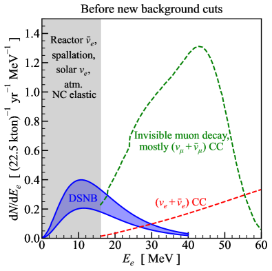
Figure 1: Schematic Super-K DSNB search. The example DSNB signal has a 6-MeV effective temperature after neutrino mixing Horiuchi et al. (2009). The example atmospheric-neutrino backgrounds, which depend on detector energy resolution and detection efficiency, are shown by Super-K’s stage-I fits Bays et al. (2012); Abe et al. (2021).

Figure 1 illustrates how the DSNB signal is presently obscured by detector backgrounds (e.g., radioactivities induced by muon spallation) and foregrounds (interactions induced by other neutrinos, which we hereafter call backgrounds, following common usage). The basic physics of these backgrounds is known, but the details are not. In the present DSNB analysis window, 16–90 MeV in electron total energy $E_{e}$, the dominant backgrounds are due to atmospheric-neutrino interactions with oxygen nuclei Malek et al. (2003); Bays et al. (2012); Zhang et al. (2015); Abe et al. (2021); below 16 MeV, several backgrounds contribute Li and Beacom (2014, 2015a, 2015b); Zhang et al. (2016); Wan et al. (2019); Locke et al. (2021); Sakai et al. (2023); Nairat et al. (in preparation). The larger atmospheric component (“the bump”) is due to the at-rest decays of invisible (sub-Cherenkov) muons, mostly produced by the charged-current (CC) interactions of ($\nu_{\mu}+\bar{\nu}_{\mu}$). The smaller component (“the ramp”) is mostly due to the CC interactions of $\nu_{e}+\bar{\nu}_{e}$. The DSNB signal and atmospheric-neutrino background rates are $\sim$ 2–4 and $\sim 50$ events/yr in 16–90 MeV. Better understanding the backgrounds will lead to new cuts to reduce them.

In this paper, we perform the first detailed calculations of atmospheric-neutrino backgrounds for DSNB searches, going well beyond earlier theoretical work Beacom and Vagins (2004); Bell et al. (2020) as well as the empirical treatment employed by Super-K in Refs. Malek et al. (2003); Bays et al. (2012); Zhang et al. (2015), where they fit the normalizations of the backgrounds to data. More recently, in Ref. Abe et al. (2021), they mention modeling the backgrounds, but almost no details or results are reported. We model the atmospheric-neutrino fluxes and their mixing, the neutrino-nucleus interactions in water, how the produced particles propagate and register in the detector, and the effects of Super-K data cuts. We take into account several effects, quantify uncertainties, and compare to data. We focus on atmospheric-neutrino CC interactions and certain high-energy NC interactions that produce events in 16–90 MeV, showing that we can also match the data at higher energies. Our results will also be useful for SK-Gd (with added gadolinium to enhance neutron detection, which began in 2020 Beacom and Vagins (2004); Abe et al. (2022); Harada et al. (2023)) and Hyper-Kamiokande Abe et al. (2018a), as well as other water Cherenkov detectors, e.g., ANNIE Anghel et al. (2015); Fischer and Weinstein (2020) and WATCHMAN Askins et al. (2015).

In Sec. II, we review the broad range of inputs needed for this work. In Sec. III, we show that our calculations reasonably reproduce the most relevant high-energy Super-K atmospheric-neutrino data, an important check. In Sec. IV and Sec. V, we show that our calculations also reasonably reproduce Super-K data in the range 16–90 MeV. This, along with our detailed accounting of the inputs and uncertainties, is our main result. In Sec. VI, we calculate the parent-particle spectra of the atmospheric-neutrino backgrounds, which provide important physical insights. In Sec. VII, we point out key actions to be taken for progress. We conclude in Sec. VIII. In a forthcoming paper Zhou and Beacom (in preparation), we detail how low-energy atmospheric events register in Super-K, which will improve how well they can be identified and controlled.

II Framing the Problem

In this section, we first review the expected DSNB signal and the observed backgrounds in Super-K. We then discuss how the atmospheric-neutrino backgrounds are formed, taking into account their fluxes and mixing, their interactions, and how these events register in the detector. Though many of these points are known, this detailed synthesis is new.

II.1 Predicted DSNB signals

The DSNB is a guaranteed flux, time-independent and isotropic, of all neutrino species Beacom (2010). Once detected, it will provide new information on the core-collapse mechanism as well as the cosmic core-collapse rate. Moreover, as core collapses that directly produce black holes have neutrino signals comparable to or larger than those that produce successful supernovae Nakazato et al. (2008); Lunardini (2009), the DSNB probes also the rate of failed supernovae Kochanek et al. (2008); Lien et al. (2010); Ashida and Nakazato (2022). If the DSNB flux is not found after modest improvements in sensitivity, then there must be surprising new physics or astrophysics.

As an example DSNB model, we use one of the predictions from Ref. Horiuchi et al. (2009) as an illustration. This model has a relatively optimistic choice of spectrum (6-MeV temperature) and an astrophysical normalization that is in good accord with subsequent work Lunardini and Tamborra (2012); Kresse et al. (2021); Horiuchi et al. (2021); Li et al. (2022); Libanov and Sharofeev (2022). There are three major inputs for the DSNB signal Beacom (2010): the neutrino emission per core collapse Ott et al. (2018); Roberts et al. (2016); Nakamura et al. (2016), the cosmic core-collapse rate Hopkins and Beacom (2006); Madau and Dickinson (2014), and the physics of detection Malek et al. (2003); Bays et al. (2012); Zhang et al. (2015); Abe et al. (2021). The first is the primary observable, as it can only be measured by neutrino experiments; it is the most uncertain. The second can be determined by electromagnetic observations, and is relatively well known. The third is very well known.

Neutrino mixing in the DSNB signal is included implicitly, as we consider only the effective neutrino spectrum outside the supernova, after all mixing effects have occurred (for active neutrinos, no mixing occurs outside the supernova because neutrinos emerge from the dense matter as incoherent mass eigenstates) Dighe and Smirnov (2000). The measured spectrum can thus be directly compared to the SN 1987A data. It is a separate problem to relate the observed spectra to the initial neutrino spectra inside the proto-neutron star.

The DSNB flux is obtained from a cosmological line-of-sight integral, with the uncertainties due to cosmological parameters being negligible. The energy-integrated flux is $\sim 10$ cm^-2 s^-1 per flavor for nominal models. The dominant contribution arises around redshift $z\sim 1$, due to the corresponding star-formation rate being $\sim 10$ times larger than the present rate and due to the contribution from higher redshifts being suppressed by the detector analysis threshold being comparable to the neutrino average energy at emission (where $\langle E\rangle\simeq 3T$, with $T$ the temperature). Currently, the best prospects for detecting the DSNB are for $\bar{\nu}_{e}$ in Super-K, due to the large cross section and the huge, low-background detector. The cross section Vogel and Beacom (1999); Strumia and Vissani (2003) is $\sigma(E_{\nu})\simeq 10^{-43}{\rm\ cm}^{2}(E_{\bar{\nu}_{e}}-1.3{\rm\ MeV})^{2}$, with the outgoing electron (hereafter, we use electron to mean electrons or positrons, unless we specify otherwise) carrying $E_{e}\simeq E_{\bar{\nu}_{e}}-1.3{\rm\ MeV}$ and being emitted near-isotropically.

II.2 Observed backgrounds in Super-K

For Super-K data, we focus on stages I–IV, for which the key DSNB search paper is Ref. Abe et al. (2021), building on prior work in Refs. Malek et al. (2003); Bays et al. (2012); Zhang et al. (2015). The energy resolution and detection efficiency vary from stage to stage, which we take into account. While added gadolinium (relevant to later data) will help with signal selection and background rejection (see Sec. II.5), the pure-water data is important because it corresponds to 15.9 livetime years. The Super-K stage IV data (more than 8 livetime years) are especially important because advances in the electronics have allowed Super-K to save detailed information on all photomultiplier (PMT) hits. This data can thus be reanalyzed as the physical understanding of the signals and backgrounds improves.

Super-K must contend with multiple backgrounds. Below 16 MeV, the backgrounds are due to reactor- and solar-neutrino interactions, spallation beta decays, and atmospheric-neutrino NC interactions. While their rates are presently large, these backgrounds can be greatly reduced with added gadolinium Beacom and Vagins (2004); Abe et al. (2022); Harada et al. (2023) (see Sec. II.5). In 16–90 MeV, while the backgrounds are substantial, they are not prohibitive. It is a remarkable achievement that the rate for these backgrounds is only about one event per week ($\sim 1.5\times 10^{-6}$ Hz). For comparison, the low-energy trigger rate is $\sim 10$ Hz, the cosmic-ray muon rate is $\sim 2$ Hz, and the rates of identified solar and higher-energy atmospheric-neutrino events are each $\sim 25$ per day ($\sim 3\times 10^{-4}$ Hz) Fukuda et al. (2003); Ashie et al. (2005a); Hosaka et al. (2006); Cravens et al. (2008); Abe et al. (2011a); Richard et al. (2016a); Abe et al. (2016).

Figure 1 shows the two components of the observed atmospheric-neutrino background: the bump and the ramp. The bump component is due to electrons from muon decay at rest, where these muons are produced with kinetic energies below the Cherenkov threshold, and hence are invisible in Super-K (visible muons are easily cut). These invisible muons are mostly produced by sub-GeV atmospheric ($\nu_{\mu}+\bar{\nu}_{\mu})$ interactions with oxygen and sometimes hydrogen nuclei. Below, we show that there is also a moderate contribution due to NC interactions of all-flavor neutrinos up to a few GeV. Once the muons decay, the isotropically emitted electrons constitute a background for the DSNB. While muon decays occur after a delay of a few microseconds, the time of the initial neutrino interaction is unknown unless a nuclear de-excitation gamma ray is produced, in which case the entire event can be recognized as a background and cut. The muon-decay spectrum shape is well known, but its normalization is not known a priori. We predict it (see Sec. IV).

The ramp component is due to promptly produced electrons from atmospheric $(\nu_{e}+\bar{\nu}_{e})$ CC interactions. This component is less important than the bump component, and it can be fit from the 60–90 MeV data, which is important to separating the ramp and bump components. Neither its spectrum shape or normalization is known a priori, though the shape seems to be simple. We predict it and the spectrum shape (see Sec. V).

II.3 Atmospheric-neutrino fluxes and mixing

To study the backgrounds induced by atmospheric neutrinos, we need the incoming fluxes and their uncertainties. For the DSNB backgrounds, the most important contributions are from neutrino energies below several GeV, and typically well below this. Atmospheric neutrinos are created through cosmic-ray interactions in the air, producing secondaries, including pions and kaons, which decay in flight, producing neutrinos Gaisser and Honda (2002); Gaisser (2005); Wendell and Okumura (2015). In this energy range, the main production mechanism is the decays of pions ($\pi^{+}\rightarrow\mu^{+}+\nu_{\mu}$ and its charge conjugate) and muons (from pion decay; $\mu^{+}\rightarrow e^{+}+\nu_{e}+\bar{\nu}_{\mu}$ and its charge conjugate). At low energies, the flux ratio (combining neutrinos and antineutrinos) is $\nu_{e}:\nu_{\mu}:\nu_{\tau}\simeq 1:2:0$ before neutrino mixing. Above several GeV, the $\nu_{e}$ fraction decreases due to some muons reaching the ground before decaying.

For the atmospheric-neutrino fluxes, we use those of Ref. Honda et al. (2015) for $E_{\nu}>100$ MeV and those of Ref. Battistoni et al. (2005) for 10–100 MeV, both evaluated at the location of Super-K. These join reasonably well; we do not adjust the normalizations so that the size of the mismatch can be judged in context of the whole spectrum. These fluxes are in reasonable accord with those in more recent work, e.g., Ref. Zhuang et al. (2022). Because we consider a long time period for Super-K stages I–IV, we use the atmospheric-neutrino flux averaged over the solar cycle; in future work, it would be interesting to take the expected flux variations into account. The neutrino flux uncertainties mostly arise from those of the primary CR flux and hadronic secondary production. To be conservative, the neutrino flux uncertainties that we adopt, following comparisons of the values quoted in Refs. Battistoni et al. (2005); Honda et al. (2007); Barr et al. (2006), are $\sim 25\%$ for 10–100 MeV, $\sim 20\%$ for 0.1–1 GeV, and $\sim 15\%$ for 1–10 GeV. These uncertainties should improve in the near future. A recent paper, Ref. Evans et al. (2017), finds smaller uncertainties in light of new cosmic-ray measurements, but its flux predictions do not yet cover the full energy range we need.

Before entering Super-K, these neutrinos undergo mixing, which depends on energy and baseline (and thus the zenith angle of the neutrino direction). The dominant effects are due to maximal $\nu_{\mu}\rightarrow\nu_{\tau}$ vacuum oscillations with the (large) atmospheric mass-squared splitting, which push the flavor ratios toward $\nu_{e}:\nu_{\mu}:\nu_{\tau}\simeq 1:1:1$, after which oscillations with the (small) solar mass-squared splitting have little effect. With increasing energy and baseline, Earth matter effects become important. We calculate the full three-flavor mixing effects (vacuum and matter) using nuCraft Wallraff and Wiebusch (2015), which computes zenith-angle, energy, and production-height dependent mixing probabilities by direct numerical integration. The uncertainties due to oscillation parameters Capozzi et al. (2017); Gariazzo et al. (2018) are smaller than those on the flux.

II.4 Neutrino interactions in water

For the DSNB signal, which ranges up to a few tens of MeV, the most important interaction is $\bar{\nu}_{e}+p\rightarrow e^{+}+n$ on free (hydrogen) protons. Interactions with nuclei are suppressed by binding effects due to the low neutrino energies and interactions with electrons are suppressed by their small masses. The signal detection cross section is well understood Vogel and Beacom (1999); Strumia and Vissani (2003).

For atmospheric neutrinos, which range from several tens of MeV to a peak in the GeV range to a falling spectrum at higher energies, the dominant interactions are with bound nucleons in oxygen. Except at the lowest neutrino energies, interactions with hydrogen are suppressed by the low number density.

In the simplest description, the two most important CC interactions that form backgrounds to the DSNB signal are $\nu_{\mu}+\,^{16}{\rm O}\rightarrow\mu^{-}+\,^{15}{\rm O}+p$ and $\bar{\nu}_{\mu}+\,^{16}{\rm O}\rightarrow\mu^{+}+\,^{15}{\rm N}+n$, where these are interactions with bound nucleons that are ejected as they are transformed by the CC weak interaction. The underlying physics of the initial neutrino-nucleon interaction may be through quasi-elastic scattering (QES), as just described, which is dominant for $E_{\nu}\lesssim 1$ GeV. At higher energies, up to $E_{\nu}\sim$ a few GeV, resonance production (RES), in which the nucleon is briefly excited to a delta resonance, is dominant. At still higher energies, deep inelastic scattering (DIS), in which the neutrino interacts with quarks, becomes dominant. These energy ranges indicate approximate guideposts, not sharp separations. We show below that for the atmospheric-neutrino events we focus on, CCQES interactions are dominant, with some contributions due to NCRES.

In slightly more detail, neutrino-nucleus interactions (both CC and NC) in this energy range are assumed to occur in two steps. First, a neutrino interacts with a single bound nucleon that has an initial momentum due to its Fermi motion. Interactions with pairs of nucleons (also called 2p/2h interactions) are also important but are less common. The interaction with the initial nucleon(s) can be affected by nuclear shadowing, and the availability of final states for the struck nucleon(s) can be affected by Pauli blocking. Second, the struck (and possibly transformed) nucleon(s), along with any other produced hadrons, travel through the nucleus, where they may interact. This is called intranuclear hadron transport or final-state interactions and it complicates the whole picture of neutrino-nucleus interactions Golan et al. (2012a); Dytman and Meyer (2011).

Because neutrino-nucleus interactions are complex and hard to handle analytically, we simulate them using GENIE, which provides a comprehensive framework Andreopoulos et al. (2010); GEN (a, b). GENIE takes into account the neutrino-nucleon/nucleus interaction vertices, nuclear effects, hadronization, final-state interactions, de-excitations of the final-state nucleus, and more, though all approximately. For the 2p/2h interactions, it uses a meson-exchange-current (MEC) model. A GENIE model set is a comprehensive model configuration (CMC) with a specific tune GEN (c). A CMC sets the models and parameters for the above physical aspects, while each CMC has several different tunes, selected to fit varying choices of datasets (neutrino-, electron-, and hadron-nucleus scattering data). The results from GENIE are surely not perfect, but they are adequate to guide our exploration of the physics of the interaction, how to improve cuts, and how to identify where new inputs are needed. In future work, it would be interesting to compare results using other neutrino-nucleus cross section codes, such as ACHILLES Isaacson et al. (2023), GIBUU Buss et al. (2012), NEUT NEU , NuWro Golan et al. (2012b), etc.

We use GENIE (v3.02.02) GEN (b) with two different model sets. The first, which is a priori expected to be more accurate, is “G18_10a_02_11b,” where “G18_10a” is the CMC name and the remainder is the tune name GEN (d). The “G18_10a” CMC embeds the best theoretical modeling elements implemented in GENIE so far GEN (a). It uses the local Fermi gas nuclear model (LFG) and an implementation of the theory calculation in Ref. Nieves et al. (2004) by Nieves, Amaro, and Valverde (NAV) for the CCQES and CC multi-nucleon processes (with Coulomb corrections included). The empirical GENIE MEC model is used for the NC multi-nucleon processes since they are not included in the calculation of Ref. Nieves et al. (2004). Hereafter, we refer to this model set simply as LFG-NAV.

For comparison, we also use the “G18_02a_00_000” model set, for which the CMC is based on the default CMC used in GENIE v2. It uses a relativistic Fermi gas nuclear model (RFG) modified by Bodek and Ritchie to incorporate short-range nucleon-nucleon correlations Bodek and Ritchie (1981). For CCQES, it uses the Llewellyn-Smith model Llewellyn Smith (1972) (LS; with Coulomb corrections not included). The empirical GENIE MEC model is used for both CC and NC multi-nucleon processes; it is known that this makes the cross sections somewhat too large Dyt . Hereafter, we refer to this model set simply as RFG-LS.

Both CMCs use the Berger-Sehgal model Berger and Sehgal (2007) for NC and CC resonance production, the Bodek-Yang model Bodek and Yang (2002) for the NC and CC shallow and deep inelastic scattering, the Berger-Sehgal model Berger and Sehgal (2009) for NC and CC coherent production of pions, the AGKY model Yang et al. (2009) for hadronization, and the INTRANUKE/hA 2018 model for final-state interactions. Other important nuclear effects are also included, including Pauli blocking, shadowing, anti-shadowing, EMC effect, de-excitation, etc. For more details, see Refs. GEN (a, c).

The neutrino-nucleus cross sections relevant to this work have large uncertainties that are not fully quantified, due to deficiencies on both the experimental and theoretical sides. We assume overall uncertainties of $\sim 20\%$ in this energy range, based on Refs. Aharmim et al. (2006); Richard et al. (2016b).

II.5 Physics of detection in Super-K

Super-K is a cylinder of diameter 39.3 m and height 41.4 m, filled with 50 ktons of ultrapure water Fukuda et al. (2003). The optically isolated inner detector has a mass of 32 kton, and its fiducial volume has a mass of 22.5 kton. Super-K detects Cherenkov light from relativistic charged particles via $\sim 11,000$ 50-cm PMTs that view the inner detector (the outer detector is viewed by a smaller number of smaller PMTs, providing an active veto layer). The inner-detector PMTs cover $\simeq 40\%$ (in Super-K stage II, it was $\simeq 20\%$, which worsened the energy resolution) of the detector wall, are sensitive to photons of wavelength $\simeq 300$–700 nm, and have a quantum efficiency of $\sim 0.1$. Below, we give more details about stage-dependent detector properties such as the energy resolution and efficiency. Very roughly, at the relevant energies, the energy resolution is $\lesssim 12\%$ ($\lesssim 18\%$ for Super-K stage II) and improving with increasing energy, while the efficiency is $\sim 90\%$ (except for Super-K stage IV at some energies, as discussed in Sec. IV.1.4).

We manage most of the detection-related calculations with our own codes. Where the physics is more complex, we simulate or check our results using FLUKA Ferrari et al. (2005), which provides a comprehensive framework for particle transport in varying media, covering particle creation, interactions and energy loss, decay and capture, and more. Here, our main use of FLUKA is the propagation of nuclear gamma rays, charged pions, and muons from neutrino interactions in water. In Ref. Zhou and Beacom (in preparation), where we detail detection signatures, we use FLUKA extensively.

To emit Cherenkov radiation, a charged particle’s speed must exceed the phase velocity of light in water, which is $c/n$, where $n\simeq 1.33$ is the refractive index of water and $c$ is the speed of light in vacuum. This sets a theoretical threshold for the lowest-speed particles that can be detected, $\beta_{th}=1/n\simeq 0.75$, or a Lorentz factor $\gamma_{th}\simeq 1.51$. For electrons, muons, pions, and protons, this corresponds to kinetic energies of 0.26, 54, 72, and 481 MeV, respectively. In practice, to be detectable, the kinetic energies must be somewhat higher, as discussed in Sec. IV.1.4. The Cherenkov angle, $\theta_{c}$, is $\cos{\theta_{c}}=1/n\beta$. For ultrarelativistic particles, $\theta_{c}=42^{\circ}$ is constant, while the angle is less for less-relativistic particles.

The pattern of PMT hits from a particle — ideally, forming a clear ring-like pattern — gives information on its type, position, energy, and direction. Its charge cannot be determined from the Cherenkov light alone. To set some relevant scales, for relativistic electrons, the light yield corresponds to about 6 detected photoelectrons per MeV and the threshold for solar-neutrino searches is $E_{e}\simeq 4$ MeV. For relativistic charged particles at higher energies, the efficiency of detection is near-perfect (this may be lowered by analysis cuts) and particle identification is very good.

Some nonrelativistic charged particles are detectable. For example, while sub-Cherenkov muons and charged pions are themselves invisible, their decays or nuclear captures almost always produce detectable signals. Also, the initial production of sub-Cherenkov muons or charged pions can be accompanied by nuclear gamma rays or neutrons. And even though neutral particles are invisible themselves, they can lead to detectable signals. Gamma rays produce detectable electrons through Compton scattering and pair production. Neutral pions quickly decay to gamma rays. Neutrons produce gamma rays through inelastic interactions with nuclei or their eventual captures on nuclei. In addition, unstable nuclei that later beta decay can be produced at the initial vertex or through particle propagation. Further details are discussed in our forthcoming paper Zhou and Beacom (in preparation).

The physical basis we use to separate DSNB signals from atmospheric-neutrino backgrounds is that DSNB $\bar{\nu}_{e}$ events produce only one electron and one neutron (the latter only detected efficiently in the presence of gadolinium), while atmospheric-neutrino events often produce different final states. The DSNB event sample is defined by several key cuts in Super-K analyses, which we follow as closely as possible when simulating neutrino interactions with GENIE and final-state particle transport with FLUKA. Events must be contained in the fiducial volume with no activity outside. The Cherenkov radiation should be only one ring, which is fuzzy due to being caused by an electron as opposed to other particles, and its angle should be about $42^{\circ}$. For the time structure, there should be only one peak (due to the decay electron), with no other activity for tens of microseconds before or after. These considerations, along with related ones for higher-energy events, help us define event classes to reproduce the Super-K data (Secs. III, IV, and V), and identify new ways to reduce backgrounds Zhou and Beacom (in preparation).

Though we focus on the pure-water data from Super-K in stages I–IV, we note that starting in 2020, Super-K began upgrading to SK-Gd by adding dissolved gadolinium sulfate, Gd₂(SO₄)₃ Beacom and Vagins (2004); Abe et al. (2022); Harada et al. (2023). In 2020, the concentration of gadolinium by mass was set to 0.01%; in 2022, it was increased to 0.03%; it may ultimately reach the originally proposed target of $0.1\%$, near which 90% of neutrons capture on gadolinium Beacom and Vagins (2004). In pure-water data, a neutron captures on a free proton, releasing a 2.2-MeV gamma ray nnd , which is hard to detect Zhang et al. (2015); Abe et al. (2021). With gadolinium, which has a huge cross section for thermal-neutron capture, the energy release is a total of $\simeq 8$ MeV in a few gamma rays nnd , which is easy to detect. The ability to tag neutrons identifies the DSNB signal (with one neutron) and rejects many backgrounds that have zero or multiple neutrons Beacom and Vagins (2004); Abe et al. (2022); Harada et al. (2023). Further progress on background rejection will come from improved spallation cuts Li and Beacom (2014, 2015a, 2015b); Zhang et al. (2016); Locke et al. (2021); Nairat et al. (in preparation) and better reconstruction of atmospheric-neutrino neutral-current (NC) events Wan et al. (2019); Sakai et al. (2023). The long-term goal is to suppress the background down to $\simeq 10$ MeV, below which reactor neutrino backgrounds will remain overwhelming.

III Calculation Validation by Matching Super-K High-Energy Atmospheric-Neutrino Data

In this section, we show that our calculations reasonably reproduce the most relevant GeV-range Super-K atmospheric-neutrino data Ashie et al. (2005b). This is a precondition to accurately predicting the low-energy (16–90 MeV) backgrounds for DSNB searches.

For the high-energy comparison, we use electron-like and muon-like data from Super-K stage I, spanning from April 1996 to July 2001 (4.1 years livetime, 22.5-kton fiducial volume). These data are near-ideal: the detection efficiency is near unity, the momentum and angular resolution values are smaller than Super-K’s bin widths, the particle identification is very good, and backgrounds are negligible. In the energy range we focus on, the physical final states and detectable event classes are relatively simple. Because our focus is on neutrino-nucleus interactions, we use Super-K’s angle-averaged spectra; the zenith-angle distributions mostly test neutrino mixing. For the Super-K data, there is a more recent paper with a much larger exposure Richard et al. (2016b), but it does not provide the charged-lepton spectra we need, instead providing only model-dependent reconstructed neutrino spectra (which our results agree with; not shown).

We focus on comparing to the angle-averaged momentum spectra of Super-K’s fully contained (FC) single-ring events, which dominate below about 1 GeV Ashie et al. (2005b). First, this energy range is closest to what we need for the calculations in Sec. IV and Sec. V. Second, then the charged leptons travel distance ranges are small compared to the detector’s size (e.g., muons travel only $\simeq 5\,{\rm m}\,(E/1\,\rm GeV)$ and electrons much less), so that the detector geometry can be ignored. For ($\nu_{e}+\bar{\nu}_{e}$), the Super-K FC event spectra start at a momentum of 0.1 GeV, while for ($\nu_{\mu}+\bar{\nu}_{\mu}$), they start at a momentum of 0.18 GeV.

The momentum spectrum of a particle $f$ can be calculated by summing the interaction channels over neutrino species, $\nu$, and targets, $T$,

$$\frac{dN_{f}}{dp_{f}}=\Delta t\sum_{\nu T\rightarrow f}N_{T}\int dE_{\nu}\,\frac{d\sigma_{\nu T\rightarrow f}}{dp_{f}}(E_{\nu},p_{f})\\ \int d\Omega_{z}\,\frac{d\Phi}{dE_{\nu}}(E_{\nu},\cos\theta_{z},\phi_{z})\,P_{\rm osc}(E_{\nu},\cos\theta_{z})\,,$$ (1)

where $\Delta t$ is the exposure time, $N_{T}$ the number of targets in the fiducial volume ($N_{\rm O}=7.5\times 10^{32}$, $N_{\rm H}=1.5\times 10^{33}$, and $N_{e}=7.5\times 10^{33}$, though interactions with electrons are negligible), and $\Omega_{z}(\cos{\theta_{z}},\phi_{z})$ is the solid angle defined with the zenith as the axis direction. The initial atmospheric-neutrino flux is ${d\Phi}/{dE_{\nu}}$, where we ignore absorption in Earth due to the low neutrino energies. The oscillation probability is $P_{\rm osc}(E_{\nu},\cos\theta_{z})$; the convolution of this with the flux over angles gives the neutrino flux after mixing. Then convolution with the differential cross section, ${d\sigma_{\nu T\rightarrow f}}/{dp_{f}}$, gives our prediction for the angle-averaged detected event spectrum.

We calculate the differential CC cross sections using GENIE simulations. For simplicity, here we calculate these without regard to Super-K’s event classes, meaning that we capture the full CC neutrino-interaction rate (NC contamination is minimal). Therefore, at sufficiently high energies, our prediction (for the total spectrum) will exceed the Super-K data (where we select the FC events only). For the event classes we neglect, these start to become important above 1 GeV. For both electron-like and muon-like events, there are contributions from multi-ring events, for which only the total visible energy is measured. And for muon-like events only, there is also a contribution from partially contained events, for which only the total contained energy is measured. As noted below, we show the energy ranges where our results should be accurate.

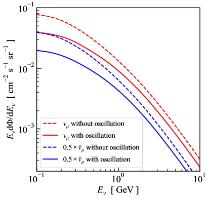
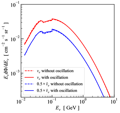
Figure 2: Angle-averaged fluxes of atmospheric neutrinos, without and with neutrino mixing, following Refs. Battistoni et al. (2005); Honda et al. (2015); Wallraff and Wiebusch (2015). We have smoothed out some small wiggles due to the discreteness of the HKKM tables. Left: Results for $\nu_{\mu}$ and $\bar{\nu}_{\mu}$. Right: Results for $\nu_{e}$ and $\bar{\nu}_{e}$ (note the change in the energy range; the notch at 0.1 GeV is due to joining different flux predictions). For $\bar{\nu}$ in both panels, we have multiplied the fluxes by 0.5 for clarity.

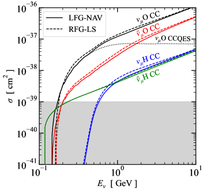
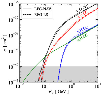
Figure 3: GENIE cross sections GEN (d) for the most important CC interactions, showing results for the two model sets used in our work (solid lines for the LFG-NAV model set and dashed lines for the RFG-LS model set). Left: Results for $\nu_{\mu}$ and $\bar{\nu}_{\mu}$. Right: Results for $\nu_{e}$ and $\bar{\nu}_{e}$ (note the change in the energy range). Below $\sim 1$ GeV, CCQES dominates, as shown for one specific channel ($\nu_{\mu}$O CCQES) in the left panel. As expected, the cross sections are somewhat larger for the RFG-LS model set. The gray shading roughly indicates the neutrino-oxygen cross section ranges that are too small to affect our results (see Figs. 7 and 8). For the neutrino-hydrogen cross section, which is more certain, somewhat smaller cross section values are relevant.

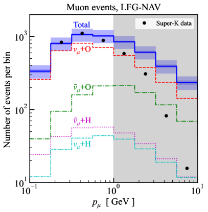
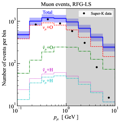
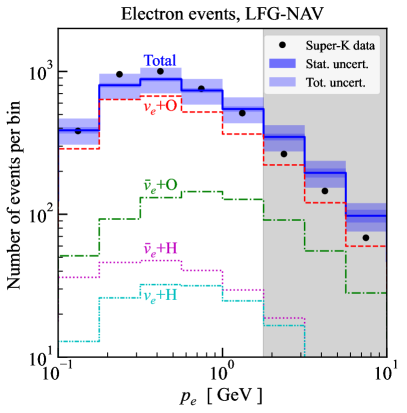
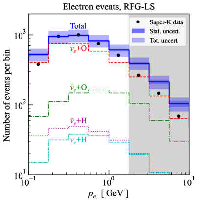
Figure 4: Our calculated results for the charged-lepton spectra induced in Super-K stage I by atmospheric neutrinos, compared to measurements (points) Ashie et al. (2005b), with the statistical and total uncertainties (i.e., statistical and systematic uncertainties added in quadrature) shown in the bands. Upper: Muon-like FC single-ring data compared to our calculations for the total rate of all event classes. In the gray region, our neglect of other event classes in the data means that our predictions should be somewhat too large. Lower: Same for electron-like events. Left: Results for the LFG-NAV model set. Right: Results for the RFG-LS model set. Both predictions agree reasonably well with data, though the RFG-LS predictions are somewhat too large at low energies, as expected.

Figure 2 shows our calculated angle-averaged atmospheric-neutrino fluxes without and with mixing (see Sec. II.3). The spectra are plotted as $EdN/dE=(2.3)^{-1}dN/d\log_{10}E$, matching the log scales on the x-axes, so that relative heights of the curves at different energies faithfully show their relative contributions to the integrated flux. The peaks near 0.1 GeV in neutrino energy follow from the peak near 1 GeV in the cosmic-ray spectrum and the kinematics of pion production and decay. At high energies, the spectra of $\nu_{\mu}$ and $\bar{\nu}_{\mu}$ follow the well-known power law for the parent cosmic rays, $dN/dE\sim E^{-2.7}$, while the spectra of $\nu_{e}$ and $\bar{\nu}_{e}$ are steeper due to some muons reaching the ground before decaying.

Figure 3 shows the most important CC cross sections, which we obtain from pre-computed tables for GENIE GEN (d). In the high-energy range, where the cross sections rise linearly, they are determined primarily by particle-physics considerations. In contrast, at lower energies, the steeper slope indicates the importance of nuclear effects and hence greater uncertainties. This is especially prominent in the $\nu_{e}$ and $\bar{\nu}_{e}$ cases, where effects due to the charged-lepton mass are negligible. For nuclear targets, antineutrinos have smaller cross sections than neutrinos, in part due to the cancellation between the vector and axial interactions Llewellyn Smith (1972); note that hydrogen targets are a special case due to the lack of neutrons. Below about 1 GeV, QES dominates; starting at few GeV, RES dominates because the thresholds for resonances are surpassed; and above several GeV, DIS dominates because the nucleons are resolved. The most important target is oxygen, due to its large number of nucleons compared to hydrogen; this changes only at the lowest energies, due to kinematic effects caused by the nuclear binding.

Figure 4 shows our calculated charged-lepton spectra for Super-K. The spectra are peaked, due to the convolution of the falling spectra (Fig. 2) and the rising cross sections (Fig. 3). In the shaded regions, the data include increasingly larger contributions from event classes besides FC single-ring events. In the non-shaded regions, the agreement for the LFG-NAV model set is within about ten percent, even better than predicted from uncertainties on the fluxes and cross sections. As expected, the RFG-LS model set gives a predicted spectrum that is somewhat too high, especially at the lowest energies, which is relevant to the calculations in Sec. IV and Sec. V.

Note that in Fig. 4, we do not show uncertainties on the Super-K data points. Instead, we show the full uncertainties on our predictions. The reason is that we want to compare specific models to measured data, as opposed to using the measured data to show the allowed range of models. In other figures below, we take a similar approach.

The results of this section thus show that the framework we use — neutrino flux, mixing, total and differential cross sections, and corresponding detector response — is adequate to reproduce the most relevant high-energy Super-K atmospheric-neutrino data. This increases our confidence in the results of the next section, where we continue to lower energies.

IV New Results on Super-K Low-Energy Atmospheric data: Invisible-Muon Component

In this section, we calculate our predictions for the invisible-muon component (the bump) of the atmospheric-neutrino background, the larger of the two components. Previously, in Refs. Malek et al. (2003); Bays et al. (2012); Zhang et al. (2015), the spectrum shape was predicted but the normalization was fit to data. More recently, in Ref. Abe et al. (2021), it is mentioned that the measured rate in 29.5–49.5 MeV is 88.8% as large as predicted, but no details or other results are given. The decay electrons from invisible muon decays follow the Michel spectrum, with a small distortion due to $\mu^{-}$ always undergoing atomic capture (mostly on oxygen) and decaying in orbit; the complete spectrum is well measured by Super-K using stopped cosmic-ray muons. (As discussed below, some $\mu^{-}$ also undergo nuclear capture, which we take into account.) When counting Michel electrons, we always mean in the energy range of 16–90 MeV. The electrons from muon decays are emitted isotropically because the muons are at rest (in any case, the atmospheric-neutrino flux is near-isotropic). Table 1 and Table 2 summarize all of our predictions. This is the first time that all of the inputs have been systematically addressed.

As noted, the DSNB signal consists of a single low-energy electron and no other measured detector activity before or after (in pure water, the probability of detecting the neutron capture is low Zhang et al. (2015); Abe et al. (2021)). This simplicity makes it straightforward for Super-K to cut backgrounds.

IV.1 Overview of the calculations

We calculate the muon initial momentum spectra using a formula similar to Eq. (1), but with some differences:

$$\frac{dN_{f}}{dp_{f}}=\Delta t\sum_{\nu T\rightarrow f}N_{T}\int dE_{\nu}\,\frac{d\sigma_{\nu T\rightarrow f}}{dp_{f}}(E_{\nu},p_{f})\otimes Cuts\otimes Corr\otimes Det\,\int d{\Omega_{z}}\,\frac{d\Phi}{dE_{\nu}}(E_{\nu},\cos\theta_{z},\phi_{z})P_{\rm osc}(E_{\nu},\cos\theta_{z})\,.$$ (2)

In this subsection, we explain the differences. First, there is one important difference in $\frac{d\sigma_{\nu T\rightarrow f}}{dp_{f}}(E_{\nu},p_{f})$ for low-energy atmospheric-neutrino events (Sec. IV.1.1). We then cover the three new terms: “$Cuts$” means the event classes defined from physically interpreting the Super-K analysis cuts (Sec. IV.1.2), “$Corr$” means several required physical corrections (Sec. IV.1.3), and “$Det$” means detection effects (Sec. IV.1.4).

IV.1.1 Basic GENIE results

In neutrino-nucleus interactions, the residual nucleus is often left in an MeV-range excited state whose decays include prompt gamma-ray emission. In water, these gamma rays deposit their energy via multiple Compton scattering and sometimes pair production. Through FLUKA simulations, we find that the total Cherenkov yield is a distribution, but that the equivalent electron energy is almost always greater than $0.75E_{\gamma}$. Given the typical nuclear gamma-ray energies here (nearly all above 5 MeV), nearly all of them should produce events in the energy range where Super-K’s efficiency is high (e.g., as in their solar-neutrino searches Hosaka et al. (2006); Cravens et al. (2008); Abe et al. (2011a, 2016)). In neutrino interactions that produce relativistic charged particles, this additional Cherenkov light is negligible, but it is important if the event has no other prompt signals, e.g., as in invisible-muon production by atmospheric neutrinos. When a nuclear gamma ray is detected a few microseconds before an electron, the event can be recognized as an invisible-muon background and rejected. There are uncertainties in both $Br_{\gamma}$ (the probability of emitting a nuclear gamma ray) and $\epsilon_{\gamma}$ (the probability of it leading to a detectable signal in Super-K) that are discussed further below.

For neutrino-oxygen interactions, GENIE models the nuclear gamma-ray emission based on Refs. Ejiri (1993); Kobayashi et al. (2005), for which $Br_{\gamma}\simeq 50\%$. Ref. Ejiri (1993) is a theoretical calculation based on the nuclear shell model, and it gives the nuclear gamma-ray energies and probabilities for the one-nucleon-hole $p_{1/2}$, $p_{3/2}$, and $s_{1/2}$ states reached via interactions with single nucleons. Where present, the emitted nuclear gamma rays are mostly above 6 MeV. Ref. Kobayashi et al. (2005) is an experimental measurement of the gamma-ray energies and probabilities for the specific case of the one-proton-hole $s_{1/2}$ state, which corresponds to a higher-energy nuclear excitation. While the probabilities of reaching these excitations are low (a few percent), the measured data are consistent with $Br_{\gamma}\simeq 50\%$ Ejiri (1993); Kobayashi et al. (2005). More recently, another theoretical calculation Ankowski et al. (2012) and an in-situ experimental measurement in T2K Abe et al. (2014, 2019) also both give results consistent with $Br_{\gamma}\simeq 50\%$.

In GENIE3 compared to GENIE2, MEC models to account for 2p/2h interactions were added to both the LFG-NAV and RFG-LS model sets. These 2p/2h interactions should also lead to final states with nuclear gamma rays, but GENIE does not include them. While Refs. Ejiri (1993); Kobayashi et al. (2005) consider only neutrino interactions with single nucleons (and not 2p/2h interactions), they do provide gamma-ray energies and emission probabilities for several cases where multiple nucleons are ejected due to the high nuclear excitations. The gamma-ray energies and probabilities should be similar regardless of the reason for ejecting multiple nucleons. Therefore, following those references, we assume that $\simeq 50\%$ of the MEC events have nuclear gamma-ray emission with energies above 5 MeV. This correction is moderately important for the LFG-NAV model set, as $\simeq 15\%$ of the invisible-muon events are due to the MEC component. It is more important for the RFG-LS model set, where the fraction is instead $\simeq 30\%$ (as noted above, the MEC component for the RFG-LS model set is known to be too large Dyt ).

IV.1.2 Cuts to GENIE results

We apply cuts to our simulation results (“$Cuts$” in Eq. (2)) to mimic the many cuts that Super-K applies to real data to isolate the DSNB signal. To define our background sample of invisible-muon events, the most important particles to keep track of are charged leptons, all types of pions, and nuclear gamma rays. We also cut other particles, like relativistic protons, but those are rare ($<1\%$ of events). To begin, we cut all events where the detectable energy or number of detectable particles is incompatible with the simple, low-energy DSNB signal.

For ($\nu_{\mu}+\bar{\nu}_{\mu}$) CC events, we then cut those where the muon is above its theoretical Cherenkov threshold ($p_{\mu}\simeq 120$ MeV). Muons with Cherenkov radiation will easily trigger the detector, typically giving a muon-like Cherenkov ring and also a decay electron a few microseconds later. Such events will be removed by Super-K’s cuts. We call our results at this step our “Naive” calculation. Below, we discuss how we must correct for muons that are not actually detectable because they are not far enough above the Cherenkov threshold.

When an invisible muon is produced, it could be accompanied by one or more pions, though the latter is rare. We cut all such events. For a $\pi^{0}$, it decays to two gamma rays, emitted in nearly opposite directions, due to the modest boosts, and these gamma rays pair-produce or Compton-scatter electrons. This causes two or more rings, allowing for these events to be cut. For a $\pi^{+}$ or a $\pi^{-}$ above the Cherenkov threshold, it will have Cherenkov radiation from itself and from its decay muon and then electron, which makes such events easy to identify. For a $\pi^{+}$ below the Cherenkov threshold, it will be cut due to the extra electron from its decay chain. A $\pi^{-}$ below the Cherenkov threshold mostly undergoes atomic capture and then nuclear capture Ponomarev (1973); Measday (2001); Czarnecki et al. (2014). These usually but not always give detectable signatures but, in any case, the total rate of such events is small.

Events with nuclear gamma rays are cut due to their “2-peak” timing features Bays et al. (2012), since these gamma rays are prompt after the neutrino interactions, whereas the Michel electrons are delayed by the muon decay time. We cut all GENIE invisible-muon events with nuclear gamma rays, plus appropriate fractions of the MEC events. We do not know the efficiency, $\epsilon_{\gamma}$, of Super-K cutting these gamma rays, as there is no clear documentation about this. In our calculation, we show results for both $\epsilon_{\gamma}=0\%$ and $\epsilon_{\gamma}=100\%$, then discuss what the observed data suggests.

IV.1.3 Physical corrections to GENIE results

There are three physical effects (“$Corr$” in Eq. (2)) that we need to apply to the GENIE results.

First, $\mu^{-}$ capture. Because of the long muon lifetime relative to the short energy-loss time, both $\mu^{-}$ and $\mu^{+}$ come to rest in matter. After that, $\mu^{+}$ decay, while $\mu^{-}$ undergo atomic capture, mostly on oxygen Ponomarev (1973); Measday (2001); Czarnecki et al. (2014). Then, our simulations using FLUKA Ferrari et al. (2005) show that $\simeq 21\%$ of $\mu^{-}$ undergo nuclear capture, producing a $\simeq 100$ MeV neutrino, which does not interact in the detector. Although $\mu^{-}$ nuclear captures may also eject nucleons and lead to nuclear de-excitation gamma rays, we find that they cannot mimic DSNB signal events in the energy range $E_{e}=$ 16–90 MeV. To account for $\mu^{-}$ capture, we reduce the overall yield of $\mu^{-}$ by $\simeq 21\%$, which affects only the $\nu_{\mu}$ CC events.

Second, a contribution from NC invisible $\pi^{+}$ channels that is missing in our treatment of ($\nu_{\mu}+\bar{\nu}_{\mu}$) CC events as the source of invisible muons. A $\pi^{+}$ below the Cherenkov threshold will decay to an invisible muon. Therefore, if a neutrino interaction produces an invisible $\pi^{+}$ and no other visible particles, it could mimic the DSNB signal. Such events can come from all-flavor NC interactions with oxygen or hydrogen, which we refer to as the NC$\pi^{+}$ channel (as noted above, $\pi^{-}$ undergo nuclear capture). There are negligible corrections from $\pi^{+}$ interacting before decaying and from $\pi^{-}$ decaying in flight. We call the calculations to this point our “Standard” calculation.

Third, Coulomb corrections due to outgoing charged particles being affected by the nuclear field. The distortion effects increase for low charged-particle energies or high nuclear charges, and are thus important for this and the following sections. For negatively charged particles, the Coulomb attraction lowers their outgoing momentum while increasing their production amplitude; the opposite occurs for positively charged particles.

Widely used Coulomb correction methods are the Fermi function and the effective momentum approximation (EMA) Traini et al. (1988); Giusti and Pacati (1987). The former only works well for electrons below $\sim 10$ MeV, and the latter only for scattering of ultrarelativistic electrons on nuclei. Here we use the modified EMA method Engel (1998), which works well for muons and electrons at the energies relevant to us. (It should also work well for charged pions.) In this method, the nucleus is approximated as a uniformly charged sphere with radius $R$ and the neutrino is assumed to interact at its center. The outgoing charged particles are thus initially subject to an electrostatic potential of $V=\pm 3Z\alpha/2R$, which is about 5.3 MeV for oxygen and 1.7 MeV for hydrogen. This potential induces a shift in the total energy of the charged particle, i.e.,

$$E\rightarrow E^{\rm eff}=E+V\,,$$ (3)

and a rescaling of the scattering amplitude, i.e.,

$$\mathcal{M}\rightarrow\mathcal{M}\sqrt{\frac{k_{\rm eff}E_{\rm eff}}{kE}}\,,$$ (4)

where $k$ and $k_{\rm eff}$ are the momentum of the charged particle before and after the shift, respectively. These changes are in the same sense because the invisible muons have a spectrum that rises with increasing momentum.

For the LFG-NAV model set, as the Coulomb corrections are already included in the CCQES model, we apply these corrections only to the NC $\pi^{+}$ channels. For the RFG-LS model set, we apply Coulomb corrections to all CC and NC $\pi^{+}$ channels. For the CC channels, the correction increases the number of invisible muons in the $\nu_{\mu}$+O CC channel and decreases those in the $\bar{\nu}_{\mu}$+O CC, $\bar{\nu}_{\mu}$+H CC, and NC $\pi^{+}$ channels. For the NC $\pi^{+}$ channel, which comes mostly from the decay of $\Delta$ baryons inside the nucleus, we ignore any corrections to the $\Delta$ baryons due to their large mass and short lifetime. For the $\pi^{+}$ from $\Delta$ decay, we do not apply the correction to the scattering amplitude because they are not directly produced by neutrino interactions, but we do include the energy shift. We call the calculations to this point our “Coulomb” calculation.

Figure 5: A test of the consistency of Super-K’s analysis results across all four Super-K stages. The integrated results for stage IV are significantly lower than the average of stages I–III, for which the reason is unknown. Note that the difference is not due to an overall factor; the ratio is energy dependent.

IV.1.4 Detection effects

The energy resolution and efficiency differ somewhat over Super-K stages I–IV, and we take this into account. While the energy resolution is somewhat worse in stage II due to the reduced number of PMTs, it remains good enough that it barely changes the results. The raw detection efficiency is near unity in all phases, though the analysis (or signal) efficiency is reduced by various cuts. The analysis efficiency is $\simeq 90\%$ for most energies in Super-K stages I–III, while it is $\simeq 70$–85% in stage IV Collaboration (2021). This is likely due to a new cut introduced for stage IV only Mic . This cut, which is on the average charge deposit per PMT (see Sec. VC5 and Fig. 14 in Ref. Abe et al. (2021)), reduces the efficiency of detecting higher-energy events.

Figure 5 shows a consistency test of the four Super-K stages, focusing on the bump data Abe et al. (2021), where we use the Super-K fits instead of the data for visual clarity. We correct for the different livetimes and efficiencies of each stage (including the new cut in stage IV), so that the curves for the four stages should agree. For stage IV, the integrated spectrum is lower than the average of stages I–III by $\simeq 35\%$, which has a statistical significance of $\simeq 7\sigma$. The reason for this discrepancy is unknown, but we must bear it in mind when comparing to data.

In the calculations above, we used the theoretical Cherenkov threshold, $\beta_{th}=1/n$, to assess if charged particles should be cut. However, if a charged particle does not have enough energy above the threshold, it will not actually produce enough Cherenkov photons to trigger the detector. Therefore, a practical Cherenkov threshold should be calculated. This is important because the spectra of charged particles in this energy range are rising with increasing momentum.

For Super-K, barely relativistic muons can be identified Bays et al. (2012). This works as long as the muon itself activates at least the super-low energy (SLE) trigger. This trigger has a threshold of 17–24 photoelectrons, where the precise value depends on the analysis period. We use the lowest number, 17, as it is believed that even a lower number of photoelectrons may still have a chance to be identified Mic . We convert this number of photoelectrons to a corrected threshold for $p_{\mu}$. First, we assume the number of photoelectrons equals the number of PMTs hit, as the total number of PMTs in Super-K’s inner detector, $>10^{4}$, is much larger. Considering the coverage and quantum efficiency of Super-K PMTs, this corresponds to about 340 Cherenkov photons with wavelengths $\lambda\simeq 300$–700 nm emitted by the muon. Finally, we convert the number of Cherenkov photons, $N_{\rm ph}$, to the momentum of the charged particles using Beacom and Palomares-Ruiz (2003); Workman et al. (2022)

$$\frac{d^{2}N_{\rm ph}}{dxd\lambda}=\frac{2\pi\alpha}{\lambda^{2}}\left[1-\frac{1}{\beta(x)^{2}n^{2}(\lambda)}\right]\,,$$ (5)

where $x$ is the distance that a charged particle travels, $\alpha$ the fine structure constant, $\beta(x)$ the velocity of the particle, and $n(\lambda)\simeq 1.33$ is the refractive index of water. For muons, this changes the Cherenkov threshold from $p_{\mu}\simeq 120$ MeV to $p_{\mu}\simeq 135$ MeV. For charged pions, this changes the Cherenkov threshold from 159 MeV to 176 MeV. Our calculation for the revised thresholds gives results consistent with those from practical Super-K detector simulations Che . These changes lead to increased numbers of predicted invisible-muon events.

IV.2 Summary of predictions and uncertainties

Table 1 summarizes our predicted numbers of decay electrons from invisible muons for Super-K stages I–IV for the two model sets of GENIE (LFG-NAV and RFG-LS; see Sec. II.4). For LFG-NAV, the predictions match the measurements of Super-K stages I–III quite well and are somewhat high for Super-K stage IV, likely due to the efficiency issue noted above (Fig. 5 and related text). For RFG-LS, the predictions are always higher than the measurements, especially for Super-K stage IV.

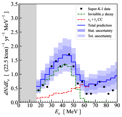
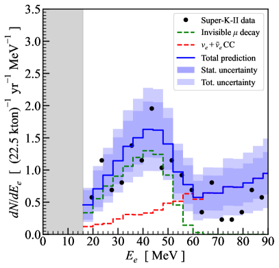
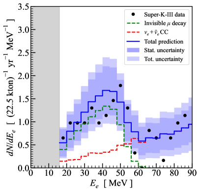
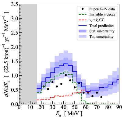
Figure 9: Same as Fig. 6, but for the RFG-LS model set. Overall, it gives a higher prediction than the data.

Figure 6 compares our LFG-NAV predictions to Super-K data in stages I–IV. (As above, we show the uncertainties on the models instead of the data.) For the invisible-muon component (the bump), we predict the normalization and the shape is known. For LFG-NAV (Fig. 6), the agreement is reasonable for all four stages, and it would not have been so without the detailed calculations above. For the RFG-LS model set (see Fig. 9 in the Appendix), the prediction is overall higher than the data for all four stages, which is expected as that MEC component is known to be too large Dyt , which explains why the LFG-NAV and RFG-LS models differ by more than the nominal $\simeq 20\%$ cross section uncertainties (Sec. II.4).

To estimate the uncertainties in our predicted yields, we consider all inputs. For the atmospheric-neutrino fluxes, we estimate the uncertainties to be $\simeq 20\%$ (Sec. II.3). For the neutrino-nucleus cross sections, we also estimate the uncertainties to be $\simeq 20\%$ (Sec. II.4). For the Cherenkov threshold correction, due to a lack of information, we estimate an uncertainty of $\simeq 20\%$. Adding these uncertainties in quadrature gives a total of $\simeq 35\%$. This is large enough to cover other uncertainties that we do not specifically note.

Table 2 shows our detailed predictions in Super-K stage IV for both the LFG-NAV and RFG-LS model sets. The results for other stages (not shown) are in similar proportions. The LFG-NAV model set embeds the best theoretical modeling elements implemented in GENIE so far GEN (a). For each model set, we show the results for the major calculational steps, represented by different columns from left to right. Until new cuts based on secondary particles are developed Zhou and Beacom (in preparation), all of the interaction channels that contribute to a given background component are indistinguishable.

• “Naive” case (Sec. IV.1.2). This is a zeroth-order approximation, with the yields of the four CC channels following their corresponding fluxes and cross sections, as in Figs. 2 and  3.

• “Standard” case (Sec. IV.1.3). We cut events with pion production and $\mu^{-}$ capture. For channels with oxygen targets, which are dominant, this removes large fractions of their events. For $\nu_{\mu}$+H CC, all events are removed due to there being no CCQES events. For $\bar{\nu}_{\mu}$+H CC, all events survive because CCQES dominates. We add NC $\pi^{+}$ channels, which contribute about 30% in the LFG-NAV model set and 20% in the RFG-LS model set, an important point that was not noted before.

• “Coulomb” case (Sec. IV.1.3). For the LFG-NAV model set, the Coulomb correction is already included in the CC channels so we apply it to the NC $\pi^{+}$ channels only. For the RFG-LS model set, we apply it to all channels. Coulomb corrections increase the yield of the $\nu_{\mu}$+O CC channel by $\simeq 35\%$ and decrease the yields of the $\bar{\nu}_{\mu}$+O CC, $\bar{\nu}_{\mu}$+H CC, and NC $\pi^{+}$ channels by $\simeq 25\%$, 10%, and 10%.

• “Threshold” case (Sec. IV.1.4). We correct the Cherenkov threshold from its theoretical value because barely relativistic charged particles may not trigger the detector. This increases the yields by $\simeq 30\%$, which is uncertain.

• Nuclear gamma rays (Sec. IV.1.2). We show two cases for the efficiency of Super-K cuts on nuclear gamma rays, as this is uncertain. We consider that either none have been removed ($\epsilon_{\gamma}=0\%$) or that all of them have ($\epsilon_{\gamma}=100\%$). To decide between these, further information from Super-K is needed.

For the nuclear gamma-ray branching ratio ($Br_{\gamma}$) and cut efficiency ($\epsilon_{\gamma}$), though they both have large uncertainties, comparing our final calculation with Super-K data gives important insights. The consistency between data and LFG-NAV prediction indicates that the choice of $Br_{\gamma}\times\epsilon_{\gamma}\simeq 50\%\times 100\%$ that we use is good. For the RFG-LS model set (Fig. 9 in Appendix A), lowering $\epsilon_{\gamma}$ would make the deviation between the prediction and the data even larger. Because we do not expect the true $Br_{\gamma}$ to be very different from $50\%$, this means that Super-K should have already efficiently cut the invisible-muon background events with nuclear gamma rays, though this is not explicitly discussed in their papers Malek et al. (2003); Bays et al. (2012); Zhang et al. (2015); Abe et al. (2021).

Table 1: Summary of the total measured (using Super-K fits Abe et al. (2021)) and predicted numbers of decay electrons ($E_{e}=$16–90 MeV) from invisible muons for Super-K stages I–IV, assuming $\epsilon_{\gamma}=100\%$. The systematic uncertainty in our prediction is about 35%. The ratios are shown in parentheses. For both model sets, the agreement is reasonable; the RFG-LS model set has some disagreement in stage IV, possibly due to the efficiency issue noted in the text.

	stage I	stage II	stage III	stage IV
Measurement	146	74	50	155
LFG-NAV prediction (ratio to measurement)	106 (0.73)	55 (0.74)	40 (0.8)	185 (1.19)
RFG-LS prediction (ratio to measurement)	148 (1.01)	77 (1.04)	57 (1.14)	259 (1.67)

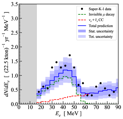
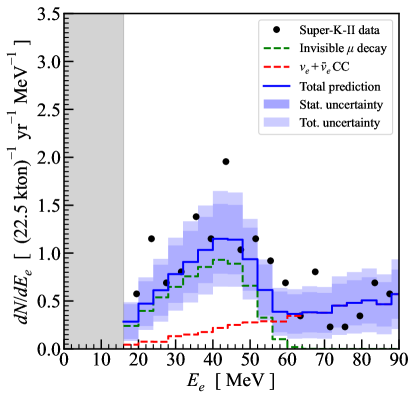
Figure 6: Our complete calculations of the atmospheric-neutrino backgrounds (using the LFG-NAV model set) compared to all four stages of Super-K data Abe et al. (2021). For the predictions, we plot the components in dashed lines and the totals in blue solid lines, with the uncertainties shown with blue bands. Although we show 4-MeV steps, we have converted the values to units of (1 MeV)^-1 (i.e., a step of height 1 contains four counts). Our calculations match the Super-K data reasonably well.

Table 2: Detailed predicted numbers of decay electrons ($E_{e}=$ 16–90 MeV) from invisible muons in Super-K stage IV. Top panel: Results for the GENIE LFG-NAV model set. Bottom panel: Results for the GENIE RFG-LS model set. Numbers in boldface are our final predictions. The columns show the steps of including various effects, concluding with the “Threshold” column. The CC channels of the LFG-NAV model set (upper table) intrinsically include Coulomb corrections, so the numbers remain unchanged when moving from the “Standard” column. We show results for two assumptions about nuclear gamma rays, where the discussion in the text favors $\epsilon_{\gamma}=100\%$. Note that while $Br_{\gamma}\simeq 50\%$, it varies between interaction channels. The total number of decay electrons passing all cuts in Super-K stage IV is 155 (from Super-K’s fits to the data) Abe et al. (2021).

Interaction channel	$Br_{\gamma}=50\%$, $\epsilon_{\gamma}=0\%$				$Br_{\gamma}=50\%$, $\epsilon_{\gamma}=100\%$
	Naive	Standard	Coulomb	Threshold	Standard	Coulomb	Threshold
$\nu_{\mu}$+O CC	159	107	107	143	56	56	75
$\bar{\nu}_{\mu}$+O CC	35	30	30	39	14	14	19
$\nu_{\mu}$+H CC	7	0	0	0	0	0	0
$\bar{\nu}_{\mu}$+H CC	24	23	23	30	23	23	30
NC $\pi^{+}$		92	84	107	51	46	61
Total	226	253	245	319	145	140	185
Total/Super-K-IV (155)	1.45	1.63	1.58	2.05	0.93	0.90	1.19

Interaction channel	$Br_{\gamma}=50\%$, $\epsilon_{\gamma}=0\%$				$Br_{\gamma}=50\%$, $\epsilon_{\gamma}=100\%$
	Naive	Standard	Coulomb	Threshold	Standard	Coulomb	Threshold
$\nu_{\mu}$+O CC	223	158	215	282	84	115	150
$\bar{\nu}_{\mu}$+O CC	48	40	29	42	20	15	20
$\nu_{\mu}$+H CC	9	0	0	0	0	0	0
$\bar{\nu}_{\mu}$+H CC	24	23	21	27	23	21	27
NC $\pi^{+}$		96	88	111	52	48	61
Total	302	317	353	461	178	198	259
Total/Super-K-IV (155)	1.94	2.04	2.27	2.96	1.15	1.27	1.67

V New results on Super-K Low-Energy Atmospheric data:
($\nu_{e}+\bar{\nu}_{e}$) CC component

In this section, we calculate our predictions for the ($\nu_{e}+\bar{\nu}_{e}$) CC component (the ramp) of the atmospheric-neutrino background, the smaller of the two components. Previously, in Super-K’s Refs. Malek et al. (2003); Bays et al. (2012); Zhang et al. (2015); Abe et al. (2021), neither the shape nor the normalization was given, though their Ref. Abe et al. (2021) mentions that modeling was done. These interactions produce a single primary electron. While these events have some directionality in principle, the low statistics and the near-isotropy of the atmospheric-neutrino flux make this hard to exploit.

Our calculation is similar to that for the invisible muon component, but there are some differences. First, here we must also take into account the atmospheric-neutrino fluxes below 100 MeV, for which we use the results of Ref. Battistoni et al. (2005). Second, here we assume that, effectively, $\epsilon_{\gamma}=0\%$ because the energy in any nuclear gamma rays (and the secondary electrons they produce) is much less than that in the primary electron from the CC interaction. Third, here no NC channels contribute.

The uncertainty in calculating the ($\nu_{e}+\bar{\nu}_{e}$) CC component is larger than for the invisible muon component. The neutrino fluxes are more uncertain because the energies are lower and because the $\nu_{e}$ and $\bar{\nu}_{e}$ fluxes arise from a further step in the decay chains, i.e., $\pi\rightarrow\mu\rightarrow e$. The neutrino cross sections are more uncertain because the interactions are more in the nuclear than the particle regime. Quantitatively, we expect the total uncertainty to be $\simeq$ 45%, arising from uncertainties in the flux (25%), cross section (30%), and Coulomb correction (20%), combined in quadrature.

Figure 6 compares our LFG-NAV predictions of the ($\nu_{e}+\bar{\nu}_{e}$) CC component to the data in Super-K stages I–IV. The spectrum rises because both the flux (Fig. 2) and cross section (Fig. 3) do. With the detailed calculations described above, the predictions from LFG-NAV (Fig. 6) agree reasonably well with the data, though the uncertainties are large. There is one peculiarity to mention. In stages I–III, the data ranged up to 90 MeV. In stage III, there are some rather high points at the highest energies. Then, in stage IV, Super-K truncated the highest energies without explanation. In fact, we recommend extending, not truncating, the range. Figure 9 in the Appendix shows the same for the RFG-LS model set, where, as for the invisible muon component, the predictions are somewhat too large.

Figure 7: Spectra of parent neutrinos for the invisible-muon component of the atmospheric-neutrino backgrounds in Super-K stage IV, calculated for the LFG-NAV model set. Left: ($\nu_{\mu}+\bar{\nu}_{\mu}$) CC component ($\simeq 70\%$ of total). Right: NC $\pi^{+}$ component ($\simeq 30\%$ of total); note changes in the axis ranges. For the RFG-LS model set, see Fig. 10 in Appendix A.

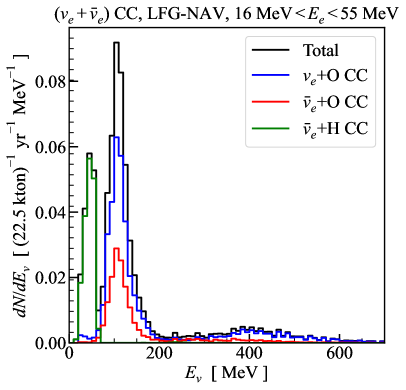
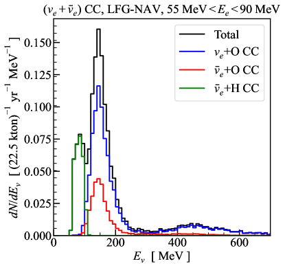
Figure 8: Spectra of parent neutrinos for the ($\nu_{e}+\bar{\nu}_{e}$) CC component of the atmospheric-neutrino backgrounds in Super-K stage IV, calculated for the LFG-NAV model set (Sec. V). Left: Results for $E_{e}=$ 16–55 MeV (45% of the total counts). Right: Results for $E_{e}=$ 55–90 MeV (55% of the total counts). For the RFG-LS model set, see Fig. 11 in Appendix A.

VI Parent Neutrino Spectra

In this section, we calculate the parent neutrino spectra for the two components of the low-energy atmospheric-neutrino backgrounds. These spectra are needed to determine how to best focus work on reducing uncertainties.

Figure 7 shows our LFG-NAV results for the invisible-muon component for Super-K stage IV. For the CC contributions (left panel), the dominant part is from $\nu_{\mu}+{\rm O}$ CC interactions, with a smaller part from $\bar{\nu}_{\mu}+{\rm O}$ CC interactions, both in the range $\simeq 100$–400 MeV, mostly due to CCQES. The small bump between $\simeq 400$ and 800 MeV is due to MEC and RES contributions. There is also a contribution from $\bar{\nu}_{\mu}+{\rm H}$ CC interactions that starts at lower energies due to having no nuclear threshold. In a simple CCQES model, the $\bar{\nu}_{\mu}+{\rm O}$ and $\bar{\nu}_{\mu}+{\rm H}$ interactions would produce neutrons that can be tagged by capture on gadolinium, while the $\nu_{\mu}+{\rm O}$ would not. However, as we show in Ref. Zhou and Beacom (in preparation), the more realistic picture is in fact more favorable, with a substantial fraction of $\nu_{\mu}+{\rm O}$ events also producing neutrons due to nuclear effects. For the NC contribution (right panel), the dominant part is from $\Delta$ resonance production that decays to a sub-Cherenkov $\pi^{+}$. The large majority of these NC events produce neutrons.

Figure 8 shows the results for the ($\nu_{e}+\bar{\nu}_{e}$) CC component. Most of the parent neutrinos are in the range 20–200 MeV, and the $\nu_{e}+{\rm O}$ channel is dominant. There is a small bump between about 300 and 600 MeV, again due to MEC and RES. The relative contributions from different channels are similar to the CC component of the invisible muons. We split the results at $E_{e}=55$ MeV, roughly where the invisible-muon and ($\nu_{e}+\bar{\nu}_{e}$) CC components of the background cross in Fig. 6.

Overall, the shapes of these spectra primarily follow from the competition between the rising charged-particle spectra at low energies and the higher probability of final states at high energies being subject to cuts. For both background components, the most striking point is that the neutrino energies are much higher than the measured electron energies. (For the signal, these are separated by only $\simeq$ 1.3 MeV.) For the invisible-muon component, this is because the electrons are produced through muon decay at rest, which obscures the initial muon energy. For the ($\nu_{e}+\bar{\nu}_{e}$) CC component, this is because the neutrino interaction rate only becomes appreciable at high enough neutrino energies; the low observed electron energies arise through the low-energy tail of the neutrino-oxygen differential cross section, plus neutrino-hydrogen interactions.

The fact that many of the background parent neutrino energies are relatively high is encouraging for cutting those events through the other secondary particles that are produced but for which cuts have yet to be devised. For example, the DSNB-induced neutrons are mostly $<1$ MeV, but atmospheric-neutrino-induced neutrons could be as energetic as 100 MeV and can travel much further Beacom and Vagins (2004). These points are detailed in our forthcoming paper Zhou and Beacom (in preparation). Knowing the parent-neutrino energy distributions is also helpful for assessing the effects of neutrino mixing and solar modulation.

VII Outline of Ways Forward

In this section, we discuss ways to reduce uncertainties on the predictions of the DSNB detector backgrounds. While our results above are adequate to start to guide strategies to reduce these backgrounds, improved precision would help. Because detection of the DSNB in Super-K is so close, even modest improvements are important. Here we focus on the most significant needs.

VII.1 Input data: atmospheric neutrino fluxes and neutrino-interaction modeling

For the atmospheric-neutrino fluxes, the uncertainties are presently $\simeq 20\%$ in the neutrino energy ranges that generate most of the DSNB backgrounds, but these uncertainties should be reducible. The flux predictions that we use — from Refs. Honda et al. (2015); Battistoni et al. (2005) — are based on old cosmic-ray data, whereas Ref. Evans et al. (2017) has shown that updating with more recent measurements can reduce uncertainties by about a factor of two. New 3D calculations using these and other contemporary inputs are needed.

For the neutrino-nucleus cross sections, the uncertainties are presently at least $\simeq 20\%$ in the most important energy ranges, but these should also be reducible. These cross sections are primarily characterized numerically through simulation codes Andreopoulos et al. (2010); Buss et al. (2012); Golan et al. (2012b); Isaacson et al. (2023); NEU that use a theoretical framework calibrated to neutrino and other scattering data, though direct neutrino-oxygen measurements Gran et al. (2006); Abe et al. (2014); Wan et al. (2019); Abe et al. (2019, 2020); Sakai et al. (2023) are scarce. These simulation codes should be updated to incorporate Coulomb and other corrections. Finally, it would be valuable for the authors of the simulation codes to compare results on a variety of predictions and to use these results to better quantify uncertainties.

It is especially important to better characterize the emission of final-state particles besides charged leptons, as this will help develop better cuts. As detailed in Sec. IV.1.1, there are significant uncertainties about nuclear gamma-ray emission; these uncertainties need to be reduced through new experimental and theoretical studies. Now that Super-K is running with added gadolinium, another critical question is about primary or secondary neutron emission, as explored in Ref. Zhou and Beacom (in preparation). The SNO (heavy water; completed) and SNO+ (light water phase; completed) experiments, while they have low rates of atmospheric-neutrino interactions, have the potential to make important measurements of gamma-ray and neutron production due to their very low background rates. Measurements with ANNIE, an accelerator neutrino experiment with a gadolinium-loaded water target, will be important for measuring both cross sections and the emission of neutrons and gamma rays Back et al. (2017, 2020).

VII.2 Super-K atmospheric analyses

New work is urgently needed on Super-K analyses of atmospheric neutrinos. (As a reminder, we focus on their pre-gadolinium data, as it has the longest exposure; first results from their DSNB search with post-gadolinium data are given in Ref. Harada et al. (2023).) One fundamental difficulty is that there are two disconnected data samples, split at roughly 100 MeV, and not quite overlapping. The higher-energy sample Ashie et al. (2005b); Wendell et al. (2010); Abe et al. (2011b); Richard et al. (2016a); Abe et al. (2018b); Jiang et al. (2019) is analyzed as a signal to measure neutrino mixing, but the lower-energy sample Malek et al. (2003); Bays et al. (2012); Zhang et al. (2015); Abe et al. (2021) is treated only as a background to the DSNB. For our purposes here, the deficiencies of the higher-energy analysis are that it uses only the cleanest events and does not adequately specify how neutrino events register in the detector. The deficiencies of the lower-energy analysis are that it does not compare to theoretical predictions (hence the need for this paper) and also does not adequately specify how neutrino events register in the detector. A new approach is needed to better connect these analyses, focusing on using all the data to accurately measure the fluxes and event rates, presenting results as a function of detected energy. For this purpose, the neutrino-mixing parameters can be taken from laboratory experiments.

It would be very helpful for future Super-K DSNB papers to provide details comparable to what we do above. In addition, key questions to resolve include:

1. For invisible-muon events with nuclear gamma rays, what are the gamma-ray probabilities and energies? For $(\nu_{e}+\bar{\nu}_{e})$ CC interactions, can nuclear gamma rays be identified?

2. How do the spectra of the low-energy events ($<$100 MeV) in detected energy connect to those at energies up through a few hundred MeV?

3. What are detection thresholds for barely relativistic muons and pions (Sec. IV.1.4)?

4. Why are the low-energy spectra observed in Super-K stage IV inconsistent with those in earlier stages (Sec. IV.1.4)?

5. Thinking ahead to future analyses, what are the details of the spallation and atmospheric NC events below 16 MeV, both before and after cuts?

Last, it would be helpful if Super-K would provide full event data for every low-energy event, as this would enable independent analyses.

VIII Conclusions

The first detection of the DSNB will be of great importance, as it will test the neutrino emission per core collapse and the cosmic core-collapse rate. Super-K is large enough to have collected $\sim 50$–100 DSNB events in total above an electron energy of $E_{e}=16$ MeV (and many more at lower energies) in its $\gtrsim 25$ years of operation, but these events are presently obscured by detector backgrounds. The largest backgrounds are due to atmospheric-neutrino interactions with nuclei. The bump component arises from the electrons produced through the decays of invisible (sub-Cherenkov) muons, and the ramp component arises from electrons produced through ($\nu_{e}+\bar{\nu}_{e}$) CC interactions.

New theoretical work is needed to better understand the physical origins of these backgrounds and how to cut them further. This matters both for reanalyzing past data as well as for making the most of new data since 2020, when Super-K began adding dissolved gadolinium to tag neutrons, which will greatly reduce detector backgrounds and allow a lower analysis threshold Beacom and Vagins (2004); Abe et al. (2022); Harada et al. (2023).

In this paper, we perform the first detailed calculations of the dominant atmospheric-neutrino backgrounds for DSNB searches in Super-K, taking into account neutrino mixing, neutrino-nucleus interactions, and how events register in Super-K. As a bottom line, our calculations can reasonably reproduce Super-K’s observed atmospheric-neutrino backgrounds in the range $E_{e}=16$–90 MeV, which are mostly produced by neutrinos in the range up to about 400 MeV. Our key results are shown in Fig. 6, Table 1, and Table 2. Achieving this agreement required taking into account several physical and detector effects, as well as checking that our calculations reasonably reproduce Super-K’s GeV-range atmospheric-neutrino data. The detailed results and comprehensive roadmap provided in this paper will help Super-K improve sensitivity to the DSNB. In our next paper Zhou and Beacom (in preparation), we go further by detailing proposed new cuts.

This program of work will not only be useful for reducing backgrounds for DSNB (and dark matter Palomares-Ruiz and Pascoli (2008); Bell et al. (2020, 2022)) searches. Put another way, Super-K has a large atmospheric-neutrino dataset below about 100 MeV that has never been exploited as a signal. The counts are large, about 50 events/year after cuts for about 25 years, so about 1250 events in total. Without cuts, these event counts would be more than a factor of two larger. Combined with data from other detectors, an exciting new frontier in low-energy atmospheric neutrinos could be opened Wan et al. (2019); Kelly et al. (2019); Newstead et al. (2021); Cheng et al. (2021a, b); Chauhan et al. (2022); Kelly et al. (2022); Denton and Pestes (2021); Zhuang et al. (2022); Kelly et al. (2023); Suliga and Beacom (2023); Sakai et al. (2023). This would allow new tests of neutrino mixing and neutrino-nucleus interactions.

Appendix A Results from the RFG-LS model set

In this section, we show our predictions from the RFG-LS model set. The predictions are larger than Super-K data and the predictions for the LFG-NAV model set, which match Super-K data better. All the figures in this section are referred to in the main text.

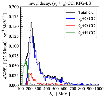
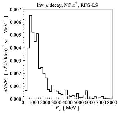
Figure 10: Same as Fig. 7, but for the RFG-LS model set.

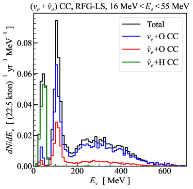
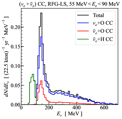
Figure 11: Same as Fig. 8, but for the RFG-LS model set.

References

- Beacom (2010) John F. Beacom, “The Diffuse Supernova Neutrino Background,” Ann. Rev. Nucl. Part. Sci. 60, 439–462 (2010), arXiv:1004.3311 [astro-ph.HE] .
- Horiuchi et al. (2009) Shunsaku Horiuchi, John F. Beacom, and Eli Dwek, “The Diffuse Supernova Neutrino Background is detectable in Super-Kamiokande,” Phys. Rev. D79, 083013 (2009), arXiv:0812.3157 [astro-ph] .
- Jeong et al. (2018) Yu Seon Jeong, Sergio Palomares-Ruiz, Mary Hall Reno, and Ina Sarcevic, “Probing secret interactions of eV-scale sterile neutrinos with the diffuse supernova neutrino background,” JCAP 06, 019 (2018), arXiv:1803.04541 [hep-ph] .
- De Gouvêa et al. (2020) André De Gouvêa, Ivan Martinez-Soler, Yuber F. Perez-Gonzalez, and Manibrata Sen, “Fundamental physics with the diffuse supernova background neutrinos,” Phys. Rev. D 102, 123012 (2020), arXiv:2007.13748 [hep-ph] .
- Das and Sen (2021) Anirban Das and Manibrata Sen, “Boosted dark matter from diffuse supernova neutrinos,” Phys. Rev. D 104, 075029 (2021), arXiv:2104.00027 [hep-ph] .
- Suliga et al. (2022) Anna M. Suliga, John F. Beacom, and Irene Tamborra, “Towards probing the diffuse supernova neutrino background in all flavors,” Phys. Rev. D 105, 043008 (2022), arXiv:2112.09168 [astro-ph.HE] .
- de Gouvêa et al. (2022) André de Gouvêa, Ivan Martinez-Soler, Yuber F. Perez-Gonzalez, and Manibrata Sen, “Diffuse supernova neutrino background as a probe of late-time neutrino mass generation,” Phys. Rev. D 106, 103026 (2022), arXiv:2205.01102 [hep-ph] .
- Bell et al. (2022) Nicole F. Bell, Matthew J. Dolan, and Sandra Robles, “Dark matter pollution in the Diffuse Supernova Neutrino Background,” JCAP 11, 060 (2022), arXiv:2205.14123 [hep-ph] .
- Akita et al. (2022) Kensuke Akita, Sang Hui Im, and Mehedi Masud, “Probing non-standard neutrino interactions with a light boson from next galactic and diffuse supernova neutrinos,” JHEP 12, 050 (2022), arXiv:2206.06852 [hep-ph] .
- Suliga (2022) Anna M. Suliga, “Diffuse Supernova Neutrino Background,” in Handbook of Nuclear Physics, edited by Isao Tanihata, Hiroshi Toki, and Toshitaka Kajino (2022) pp. 1–18, arXiv:2207.09632 [astro-ph.HE] .
- Kotake et al. (2006) Kei Kotake, Katsuhiko Sato, and Keitaro Takahashi, “Explosion mechanism, neutrino burst, and gravitational wave in core-collapse supernovae,” Rept. Prog. Phys. 69, 971–1144 (2006), arXiv:astro-ph/0509456 [astro-ph] .
- Dasgupta et al. (2009) Basudeb Dasgupta, Amol Dighe, Georg G. Raffelt, and Alexei Yu. Smirnov, “Multiple Spectral Splits of Supernova Neutrinos,” Phys. Rev. Lett. 103, 051105 (2009), arXiv:0904.3542 [hep-ph] .
- Hudepohl et al. (2010) L. Hudepohl, B. Muller, H. T. Janka, A. Marek, and G. G. Raffelt, “Neutrino Signal of Electron-Capture Supernovae from Core Collapse to Cooling,” Phys. Rev. Lett. 104, 251101 (2010), [Erratum: Phys. Rev. Lett.105,249901(2010)], arXiv:0912.0260 [astro-ph.SR] .
- Scholberg (2012) Kate Scholberg, “Supernova Neutrino Detection,” Ann. Rev. Nucl. Part. Sci. 62, 81–103 (2012), arXiv:1205.6003 [astro-ph.IM] .
- Adams et al. (2013) Scott M. Adams, C. S. Kochanek, John F. Beacom, Mark R. Vagins, and K. Z. Stanek, “Observing the Next Galactic Supernova,” Astrophys. J. 778, 164 (2013), arXiv:1306.0559 [astro-ph.HE] .
- Jana et al. (2022) Sudip Jana, Yago P. Porto-Silva, and Manibrata Sen, “Exploiting a future galactic supernova to probe neutrino magnetic moments,” JCAP 09, 079 (2022), arXiv:2203.01950 [hep-ph] .
- Segerlund et al. (2021) Manne Segerlund, Erin O’Sullivan, and Evan O’Connor, “Measuring the distance and mass of galactic core-collapse supernovae using neutrinos,” (2021), arXiv:2101.10624 [astro-ph.HE] .
- Hansen et al. (2020) Rasmus S. L. Hansen, Manfred Lindner, and Oliver Scholer, “Timing the neutrino signal of a Galactic supernova,” Phys. Rev. D 101, 123018 (2020), arXiv:1904.11461 [hep-ph] .
- Franarin et al. (2018) Tarso Franarin, Jonathan H. Davis, and Malcolm Fairbairn, “Prospects for detecting eV-scale sterile neutrinos from a galactic supernova,” JCAP 09, 002 (2018), arXiv:1712.03836 [astro-ph.HE] .
- Horiuchi et al. (2017) Shunsaku Horiuchi, Ko Nakamura, Tomoya Takiwaki, and Kei Kotake, “Estimating the core compactness of massive stars with Galactic supernova neutrinos,” J. Phys. G 44, 114001 (2017), arXiv:1708.08513 [astro-ph.HE] .
- Lu et al. (2016) Jia-Shu Lu, Yu-Feng Li, and Shun Zhou, “Getting the most from the detection of Galactic supernova neutrinos in future large liquid-scintillator detectors,” Phys. Rev. D 94, 023006 (2016), arXiv:1605.07803 [hep-ph] .
- Fischer et al. (2015) V. Fischer et al., “Prompt directional detection of galactic supernova by combining large liquid scintillator neutrino detectors,” JCAP 08, 032 (2015), arXiv:1504.05466 [astro-ph.IM] .
- Chang et al. (2023) Po-Wen Chang, Ivan Esteban, John F. Beacom, Todd A. Thompson, and Christopher M. Hirata, “Toward Powerful Probes of Neutrino Self-Interactions in Supernovae,” Phys. Rev. Lett. 131, 071002 (2023), arXiv:2206.12426 [hep-ph] .
- Kochanek et al. (2008) C. S. Kochanek, J. F. Beacom, M. D. Kistler, J. L. Prieto, K. Z. Stanek, T. A. Thompson, and H. Yuksel, “A Survey About Nothing: Monitoring a Million Supergiants for Failed Supernovae,” Astrophys. J. 684, 1336–1342 (2008), arXiv:0802.0456 [astro-ph] .
- Lunardini (2009) Cecilia Lunardini, “Diffuse neutrino flux from failed supernovae,” Phys. Rev. Lett. 102, 231101 (2009), arXiv:0901.0568 [astro-ph.SR] .
- Hidaka et al. (2015) Jun Hidaka, Grant J. Mathews, Toshitaka. Kajino, and Jutaro Suzuki, “Equation of State of Proto-Neutron Star and Failed Supernova Neutrino,” JPS Conf. Proc. 6, 030137 (2015).
- Zaizen et al. (2018) Masamichi Zaizen, Takashi Yoshida, Kohsuke Sumiyoshi, and Hideyuki Umeda, “Collective neutrino oscillations and detectabilities in failed supernovae,” Phys. Rev. D 98, 103020 (2018), arXiv:1811.03320 [astro-ph.HE] .
- Neustadt et al. (2021) J. M. M. Neustadt, C. S. Kochanek, K. Z. Stanek, C. M. Basinger, T. Jayasinghe, C. T. Garling, S. M. Adams, and J. Gerke, “The search for failed supernovae with the Large Binocular Telescope: a new candidate and the failed SN fraction with 11 yr of data,” Mon. Not. Roy. Astron. Soc. 508, 516–528 (2021), arXiv:2104.03318 [astro-ph.SR] .
- Ivanov and Fernández (2021) Mario Ivanov and Rodrigo Fernández, “Mass ejection in failed supernovae: equation of state and neutrino loss dependence,” Astrophys. J. 911, 6 (2021), arXiv:2101.02712 [astro-ph.HE] .
- Ashida and Nakazato (2022) Yosuke Ashida and Ken’ichiro Nakazato, “Exploring the Fate of Stellar Core Collapse with Supernova Relic Neutrinos,” Astrophys. J. 937, 30 (2022), arXiv:2204.04880 [astro-ph.HE] .
- Malek et al. (2003) M. Malek et al. (Super-Kamiokande), “Search for supernova relic neutrinos at SUPER-KAMIOKANDE,” Phys. Rev. Lett. 90, 061101 (2003), arXiv:hep-ex/0209028 [hep-ex] .
- Bays et al. (2012) K. Bays et al. (Super-Kamiokande), “Supernova Relic Neutrino Search at Super-Kamiokande,” Phys. Rev. D 85, 052007 (2012), arXiv:1111.5031 [hep-ex] .
- Zhang et al. (2015) H. Zhang et al. (Super-Kamiokande), “Supernova Relic Neutrino Search with Neutron Tagging at Super-Kamiokande-IV,” Astropart. Phys. 60, 41–46 (2015), arXiv:1311.3738 [hep-ex] .
- Abe et al. (2021) K. Abe et al. (Super-Kamiokande), “Diffuse supernova neutrino background search at Super-Kamiokande,” Phys. Rev. D 104, 122002 (2021), arXiv:2109.11174 [astro-ph.HE] .
- Fukuda et al. (2003) Y. Fukuda et al. (Super-Kamiokande), “The Super-Kamiokande detector,” Advanced computing and analysis techniques in physics research. Proceedings, 8th International Workshop, ACAT 2002, Moscow, Russia, June 24-28, 2002, Nucl. Instrum. Meth. A501, 418–462 (2003).
- Vogel and Beacom (1999) P. Vogel and John F. Beacom, “Angular distribution of neutron inverse beta decay, anti-neutrino(e) + p —¿ e+ + n,” Phys. Rev. D60, 053003 (1999), arXiv:hep-ph/9903554 [hep-ph] .
- Strumia and Vissani (2003) Alessandro Strumia and Francesco Vissani, “Precise quasielastic neutrino/nucleon cross-section,” Phys. Lett. B564, 42–54 (2003), arXiv:astro-ph/0302055 [astro-ph] .
- Li and Beacom (2014) Shirley Weishi Li and John F. Beacom, “First calculation of cosmic-ray muon spallation backgrounds for MeV astrophysical neutrino signals in Super-Kamiokande,” Phys. Rev. C89, 045801 (2014), arXiv:1402.4687 [hep-ph] .
- Li and Beacom (2015a) Shirley Weishi Li and John F. Beacom, “Spallation Backgrounds in Super-Kamiokande Are Made in Muon-Induced Showers,” Phys. Rev. D91, 105005 (2015a), arXiv:1503.04823 [hep-ph] .
- Li and Beacom (2015b) Shirley Weishi Li and John F. Beacom, “Tagging Spallation Backgrounds with Showers in Water-Cherenkov Detectors,” Phys. Rev. D92, 105033 (2015b), arXiv:1508.05389 [physics.ins-det] .
- Zhang et al. (2016) Y. Zhang et al. (Super-Kamiokande), “First measurement of radioactive isotope production through cosmic-ray muon spallation in Super-Kamiokande IV,” Phys. Rev. D 93, 012004 (2016), arXiv:1509.08168 [hep-ex] .
- Wan et al. (2019) L. Wan et al. (Super-Kamiokande), “Measurement of the neutrino-oxygen neutral-current quasielastic cross section using atmospheric neutrinos at Super-Kamiokande,” Phys. Rev. D 99, 032005 (2019), arXiv:1901.05281 [hep-ex] .
- Locke et al. (2021) S. Locke et al. (Super-Kamiokande), “New Methods and Simulations for Cosmogenic Induced Spallation Removal in Super-Kamiokande-IV,” (2021), arXiv:2112.00092 [hep-ex] .
- Sakai et al. (2023) S. Sakai et al., “Measurement of the neutrino-oxygen neutral-current quasielastic cross section using atmospheric neutrinos in the SK-Gd experiment,” (2023), arXiv:2311.03842 [hep-ex] .
- Nairat et al. (in preparation) O. Nairat, S. W. Li, and J. F. Beacom, (in preparation).
- Beacom and Vagins (2004) John F. Beacom and Mark R. Vagins, “GADZOOKS! Anti-neutrino spectroscopy with large water Cherenkov detectors,” Phys. Rev. Lett. 93, 171101 (2004), arXiv:hep-ph/0309300 [hep-ph] .
- Bell et al. (2020) Nicole F. Bell, Matthew J. Dolan, and Sandra Robles, “Searching for Sub-GeV Dark Matter in the Galactic Centre using Hyper-Kamiokande,” JCAP 09, 019 (2020), arXiv:2005.01950 [hep-ph] .
- Abe et al. (2022) K. Abe et al. (Super-Kamiokande), “First gadolinium loading to Super-Kamiokande,” Nucl. Instrum. Meth. A 1027, 166248 (2022), arXiv:2109.00360 [physics.ins-det] .
- Harada et al. (2023) M. Harada et al. (Super-Kamiokande), “Search for Astrophysical Electron Antineutrinos in Super-Kamiokande with 0.01% Gadolinium-loaded Water,” Astrophys. J. Lett. 951, L27 (2023), arXiv:2305.05135 [astro-ph.HE] .
- Abe et al. (2018a) K. Abe et al. (Hyper-Kamiokande), “Hyper-Kamiokande Design Report,” (2018a), arXiv:1805.04163 [physics.ins-det] .
- Anghel et al. (2015) I. Anghel et al. (ANNIE), “Letter of Intent: The Accelerator Neutrino Neutron Interaction Experiment (ANNIE),” (2015), arXiv:1504.01480 [physics.ins-det] .
- Fischer and Weinstein (2020) V. Fischer and A. Weinstein (ANNIE), “ANNIE: Neutron multiplicity in neutrino interactions and new technologies,” J. Phys. Conf. Ser. 1468, 012226 (2020).
- Askins et al. (2015) M. Askins et al. (WATCHMAN), “The Physics and Nuclear Nonproliferation Goals of WATCHMAN: A WAter CHerenkov Monitor for ANtineutrinos,” (2015), arXiv:1502.01132 [physics.ins-det] .
- Zhou and Beacom (in preparation) Bei Zhou and John F. Beacom, “ ,” (in preparation).
- Nakazato et al. (2008) Ken’ichiro Nakazato, Kohsuke Sumiyoshi, Hideyuki Suzuki, and Shoichi Yamada, “Oscillation and Future Detection of Failed Supernova Neutrinos from Black Hole Forming Collapse,” Phys. Rev. D78, 083014 (2008), [Erratum: Phys. Rev.D79,069901(2009)], arXiv:0810.3734 [astro-ph] .
- Lien et al. (2010) Amy Lien, Brian D. Fields, and John F. Beacom, “Synoptic Sky Surveys and the Diffuse Supernova Neutrino Background: Removing Astrophysical Uncertainties and Revealing Invisible Supernovae,” Phys. Rev. D81, 083001 (2010), arXiv:1001.3678 [astro-ph.CO] .
- Lunardini and Tamborra (2012) Cecilia Lunardini and Irene Tamborra, “Diffuse supernova neutrinos: oscillation effects, stellar cooling and progenitor mass dependence,” JCAP 1207, 012 (2012), arXiv:1205.6292 [astro-ph.SR] .
- Kresse et al. (2021) Daniel Kresse, Thomas Ertl, and Hans-Thomas Janka, “Stellar Collapse Diversity and the Diffuse Supernova Neutrino Background,” Astrophys. J. 909, 169 (2021), arXiv:2010.04728 [astro-ph.HE] .
- Horiuchi et al. (2021) Shunsaku Horiuchi, Tomoya Kinugawa, Tomoya Takiwaki, Koh Takahashi, and Kei Kotake, “Impact of binary interactions on the diffuse supernova neutrino background,” Phys. Rev. D 103, 043003 (2021), arXiv:2012.08524 [astro-ph.HE] .
- Li et al. (2022) Yu-Feng Li, Mark Vagins, and Michael Wurm, “Prospects for the Detection of the Diffuse Supernova Neutrino Background with the Experiments SK-Gd and JUNO,” Universe 8, 181 (2022), arXiv:2201.12920 [astro-ph.HE] .
- Libanov and Sharofeev (2022) Alexander Libanov and Andrey Sharofeev, “Diffuse supernova neutrino background in the standard and double collapse models,” Phys. Rev. D 106, 123012 (2022), arXiv:2202.01206 [astro-ph.HE] .
- Ott et al. (2018) C. D. Ott, L. F. Roberts, A. da Silva Schneider, J. M. Fedrow, R. Haas, and E. Schnetter, “The Progenitor Dependence of Core-collapse Supernovae from Three-dimensional Simulations with Progenitor Models of 12–40 M⊙,” Astrophys. J. Lett. 855, L3 (2018), arXiv:1712.01304 [astro-ph.HE] .
- Roberts et al. (2016) Luke F. Roberts, Christian D. Ott, Roland Haas, Evan P. O’Connor, Peter Diener, and Erik Schnetter, “General Relativistic Three-Dimensional Multi-Group Neutrino Radiation-Hydrodynamics Simulations of Core-Collapse Supernovae,” Astrophys. J. 831, 98 (2016), arXiv:1604.07848 [astro-ph.HE] .
- Nakamura et al. (2016) Ko Nakamura, Shunsaku Horiuchi, Masaomi Tanaka, Kazuhiro Hayama, Tomoya Takiwaki, and Kei Kotake, “Multimessenger signals of long-term core-collapse supernova simulations: synergetic observation strategies,” Mon. Not. Roy. Astron. Soc. 461, 3296–3313 (2016), arXiv:1602.03028 [astro-ph.HE] .
- Hopkins and Beacom (2006) Andrew M. Hopkins and John F. Beacom, “On the normalisation of the cosmic star formation history,” Astrophys. J. 651, 142–154 (2006), arXiv:astro-ph/0601463 .
- Madau and Dickinson (2014) Piero Madau and Mark Dickinson, “Cosmic Star Formation History,” Ann. Rev. Astron. Astrophys. 52, 415–486 (2014), arXiv:1403.0007 [astro-ph.CO] .
- Dighe and Smirnov (2000) Amol S. Dighe and Alexei Yu. Smirnov, “Identifying the neutrino mass spectrum from the neutrino burst from a supernova,” Phys. Rev. D 62, 033007 (2000), arXiv:hep-ph/9907423 .
- Ashie et al. (2005a) Y. Ashie et al. (Super-Kamiokande), “A Measurement of atmospheric neutrino oscillation parameters by SUPER-KAMIOKANDE I,” Phys. Rev. D 71, 112005 (2005a), arXiv:hep-ex/0501064 .
- Hosaka et al. (2006) J. Hosaka et al. (Super-Kamiokande), “Solar neutrino measurements in super-Kamiokande-I,” Phys. Rev. D 73, 112001 (2006), arXiv:hep-ex/0508053 .
- Cravens et al. (2008) J. P. Cravens et al. (Super-Kamiokande), “Solar neutrino measurements in Super-Kamiokande-II,” Phys. Rev. D 78, 032002 (2008), arXiv:0803.4312 [hep-ex] .
- Abe et al. (2011a) K. Abe et al. (Super-Kamiokande), “Solar neutrino results in Super-Kamiokande-III,” Phys. Rev. D 83, 052010 (2011a), arXiv:1010.0118 [hep-ex] .
- Richard et al. (2016a) E. Richard et al. (Super-Kamiokande), “Measurements of the atmospheric neutrino flux by Super-Kamiokande: energy spectra, geomagnetic effects, and solar modulation,” Phys. Rev. D 94, 052001 (2016a), arXiv:1510.08127 [hep-ex] .
- Abe et al. (2016) K. Abe et al. (Super-Kamiokande), “Solar Neutrino Measurements in Super-Kamiokande-IV,” Phys. Rev. D 94, 052010 (2016), arXiv:1606.07538 [hep-ex] .
- Gaisser and Honda (2002) T. K. Gaisser and M. Honda, “Flux of atmospheric neutrinos,” Ann. Rev. Nucl. Part. Sci. 52, 153–199 (2002), arXiv:hep-ph/0203272 [hep-ph] .
- Gaisser (2005) Thomas K. Gaisser, “Atmospheric neutrino fluxes,” Proceedings, Nobel Symposium 129: Neutrion Physics: Enkoeping, Sweden, August 19-24, 2004, Phys. Scripta T121, 51–56 (2005), arXiv:astro-ph/0502380 [astro-ph] .
- Wendell and Okumura (2015) Roger Wendell and Kimihiro Okumura, “Recent progress and future prospects with atmospheric neutrinos,” New J. Phys. 17, 025006 (2015).
- Honda et al. (2015) M. Honda, M. Sajjad Athar, T. Kajita, K. Kasahara, and S. Midorikawa, “Atmospheric neutrino flux calculation using the NRLMSISE-00 atmospheric model,” Phys. Rev. D92, 023004 (2015), arXiv:1502.03916 [astro-ph.HE] .
- Battistoni et al. (2005) G. Battistoni, A. Ferrari, T. Montaruli, and P. R. Sala, “The atmospheric neutrino flux below 100-MeV: The FLUKA results,” Astropart. Phys. 23, 526–534 (2005).
- Zhuang et al. (2022) Yi Zhuang, Louis E. Strigari, and Rafael F. Lang, “Time variation of the atmospheric neutrino flux at dark matter detectors,” Phys. Rev. D 105, 043001 (2022), arXiv:2110.14723 [hep-ph] .
- Honda et al. (2007) Morihiro Honda, T. Kajita, K. Kasahara, S. Midorikawa, and T. Sanuki, “Calculation of atmospheric neutrino flux using the interaction model calibrated with atmospheric muon data,” Phys. Rev. D75, 043006 (2007), arXiv:astro-ph/0611418 [astro-ph] .
- Barr et al. (2006) G. D. Barr, T. K. Gaisser, S. Robbins, and Todor Stanev, “Uncertainties in Atmospheric Neutrino Fluxes,” Phys. Rev. D74, 094009 (2006), arXiv:astro-ph/0611266 [astro-ph] .
- Evans et al. (2017) Justin Evans, Diego Garcia Gamez, Salvatore Davide Porzio, Stefan Söldner-Rembold, and Steven Wren, “Uncertainties in Atmospheric Muon-Neutrino Fluxes Arising from Cosmic-Ray Primaries,” Phys. Rev. D 95, 023012 (2017), arXiv:1612.03219 [astro-ph.HE] .
- Wallraff and Wiebusch (2015) Marius Wallraff and Christopher Wiebusch, “Calculation of oscillation probabilities of atmospheric neutrinos using nuCraft,” Comput. Phys. Commun. 197, 185–189 (2015), arXiv:1409.1387 [astro-ph.IM] .
- Capozzi et al. (2017) Francesco Capozzi, Eleonora Di Valentino, Eligio Lisi, Antonio Marrone, Alessandro Melchiorri, and Antonio Palazzo, “Global constraints on absolute neutrino masses and their ordering,” Phys. Rev. D95, 096014 (2017), arXiv:1703.04471 [hep-ph] .
- Gariazzo et al. (2018) S. Gariazzo, M. Archidiacono, P. F. de Salas, O. Mena, C. A. Ternes, and M. Tórtola, “Neutrino masses and their ordering: Global Data, Priors and Models,” JCAP 1803, 011 (2018), arXiv:1801.04946 [hep-ph] .
- Golan et al. (2012a) Tomasz Golan, Cezary Juszczak, and Jan T. Sobczyk, “Final State Interactions Effects in Neutrino-Nucleus Interactions,” Phys. Rev. C86, 015505 (2012a), arXiv:1202.4197 [nucl-th] .
- Dytman and Meyer (2011) S. A. Dytman and A. S. Meyer, “Final state interactions in GENIE,” Proceedings, 7th International Workshop on Neutrino-nucleus interactions in the few GeV region (NUINT 11): Dehradun, India, March 7-11, 2011, AIP Conf. Proc. 1405, 213–218 (2011).
- Andreopoulos et al. (2010) C. Andreopoulos et al., “The GENIE Neutrino Monte Carlo Generator,” Nucl. Instrum. Meth. A614, 87–104 (2010), arXiv:0905.2517 [hep-ph] .
- GEN (a) https://genie-docdb.pp.rl.ac.uk/DocDB/0000/000002/007/man.pdf (a).
- GEN (b) http://www.genie-mc.org/ (b).
- GEN (c) https://hep.ph.liv.ac.uk/~costasa/genie/tunes.html (c).
- Isaacson et al. (2023) Joshua Isaacson, William I. Jay, Alessandro Lovato, Pedro A. N. Machado, and Noemi Rocco, “Introducing a novel event generator for electron-nucleus and neutrino-nucleus scattering,” Phys. Rev. D 107, 033007 (2023), arXiv:2205.06378 [hep-ph] .
- Buss et al. (2012) O. Buss, T. Gaitanos, K. Gallmeister, H. van Hees, M. Kaskulov, O. Lalakulich, A. B. Larionov, T. Leitner, J. Weil, and U. Mosel, “Transport-theoretical Description of Nuclear Reactions,” Phys. Rept. 512, 1–124 (2012), arXiv:1106.1344 [hep-ph] .
- (94) https://www.actaphys.uj.edu.pl/fulltext?series=Reg&vol=40&page=2477.
- Golan et al. (2012b) T. Golan, J. T. Sobczyk, and J. Zmuda, “NuWro: the Wroclaw Monte Carlo Generator of Neutrino Interactions,” Nucl. Phys. B Proc. Suppl. 229-232, 499–499 (2012b).
- GEN (d) https://scisoft.fnal.gov/scisoft/packages/genie_xsec/v3_02_00/ (d).
- Nieves et al. (2004) J. Nieves, Jose Enrique Amaro, and M. Valverde, “Inclusive quasi-elastic neutrino reactions,” Phys. Rev. C 70, 055503 (2004), [Erratum: Phys.Rev.C 72, 019902 (2005)], arXiv:nucl-th/0408005 .
- Bodek and Ritchie (1981) A. Bodek and J. L. Ritchie, “Further Studies of Fermi Motion Effects in Lepton Scattering from Nuclear Targets,” Phys. Rev. D24, 1400 (1981).
- Llewellyn Smith (1972) C. H. Llewellyn Smith, “Neutrino Reactions at Accelerator Energies,” Gauge Theories and Neutrino Physics, Jacob, 1978:0175, Phys. Rept. 3, 261–379 (1972).
- (100) Steve Dytman (private communication).
- Berger and Sehgal (2007) Ch. Berger and L. M. Sehgal, “Lepton mass effects in single pion production by neutrinos,” Phys. Rev. D 76, 113004 (2007), arXiv:0709.4378 [hep-ph] .
- Bodek and Yang (2002) A. Bodek and U. K. Yang, “Modeling deep inelastic cross-sections in the few GeV region,” Nucl. Phys. B Proc. Suppl. 112, 70–76 (2002), arXiv:hep-ex/0203009 .
- Berger and Sehgal (2009) Ch. Berger and L. M. Sehgal, “PCAC and coherent pion production by low energy neutrinos,” Phys. Rev. D 79, 053003 (2009), arXiv:0812.2653 [hep-ph] .
- Yang et al. (2009) T. Yang, C. Andreopoulos, H. Gallagher, K. Hoffmann, and P. Kehayias, “A Hadronization Model for Few-GeV Neutrino Interactions,” Eur. Phys. J. C 63, 1–10 (2009), arXiv:0904.4043 [hep-ph] .
- Aharmim et al. (2006) B. Aharmim et al. (SNO), “A Search for Neutrinos from the Solar hep Reaction and the Diffuse Supernova Neutrino Background with the Sudbury Neutrino Observatory,” Astrophys. J. 653, 1545–1551 (2006), arXiv:hep-ex/0607010 [hep-ex] .
- Richard et al. (2016b) E. Richard et al. (Super-Kamiokande), “Measurements of the atmospheric neutrino flux by Super-Kamiokande: energy spectra, geomagnetic effects, and solar modulation,” Phys. Rev. D94, 052001 (2016b), arXiv:1510.08127 [hep-ex] .
- Ferrari et al. (2005) Alfredo Ferrari, Paola R. Sala, Alberto Fasso, and Johannes Ranft, “FLUKA: A multi-particle transport code (Program version 2005),” (2005), 10.2172/877507.
- (108) https://www.nndc.bnl.gov/.
- Ashie et al. (2005b) Y. Ashie et al. (Super-Kamiokande), “A Measurement of atmospheric neutrino oscillation parameters by SUPER-KAMIOKANDE I,” Phys. Rev. D71, 112005 (2005b), arXiv:hep-ex/0501064 [hep-ex] .
- Ejiri (1993) H. Ejiri, “Nuclear deexcitations of nucleon holes associated with nucleon decays in nuclei,” Phys. Rev. C48, 1442–1444 (1993).
- Kobayashi et al. (2005) K. Kobayashi et al., “Detection of nuclear de-excitation gamma-rays in water Cherenkov detector,” Proceedings, 3rd International Workshop on Neutrino-nucleus interactions in the few GeV region (NUINT 04): Assergi, Italy, March 17-21, 2004, Nucl. Phys. Proc. Suppl. 139, 72–76 (2005), [,72(2005)].
- Ankowski et al. (2012) Artur M. Ankowski, Omar Benhar, Takaaki Mori, Ryuta Yamaguchi, and Makoto Sakuda, “Analysis of -ray production in neutral-current neutrino-oxygen interactions at energies above 200 MeV,” Phys. Rev. Lett. 108, 052505 (2012), arXiv:1110.0679 [nucl-th] .
- Abe et al. (2014) K. Abe et al. (T2K), “Measurement of the neutrino-oxygen neutral-current interaction cross section by observing nuclear deexcitation rays,” Phys. Rev. D 90, 072012 (2014), arXiv:1403.3140 [hep-ex] .
- Abe et al. (2019) K. Abe et al. (T2K), “Measurement of neutrino and antineutrino neutral-current quasielasticlike interactions on oxygen by detecting nuclear deexcitation rays,” Phys. Rev. D 100, 112009 (2019), arXiv:1910.09439 [hep-ex] .
- Ponomarev (1973) L. I. Ponomarev, “Molecular structure effects on atomic and nuclear capture of mesons,” Ann. Rev. Nucl. Part. Sci. 23, 395–430 (1973).
- Measday (2001) D. F. Measday, “The nuclear physics of muon capture,” Phys. Rept. 354, 243–409 (2001).
- Czarnecki et al. (2014) Andrzej Czarnecki, Matthew Dowling, Xavier Garcia i Tormo, William J. Marciano, and Robert Szafron, “Michel decay spectrum for a muon bound to a nucleus,” Phys. Rev. D 90, 093002 (2014), arXiv:1406.3575 [hep-ph] .
- Traini et al. (1988) M. Traini, Sylvaine Turck-Chieze, and A. Zghiche, “Deep Inelastic Electron Scattering in the Distorted Wave Born Approximation: An Analytic Approach,” Phys. Rev. C38, 2799–2812 (1988).
- Giusti and Pacati (1987) C. Giusti and F. D. Pacati, “Electron distortion in quasifree (e,e?p) reactions,” Nucl. Phys. A473, 717–735 (1987).
- Engel (1998) Jonathan Engel, “Approximate treatment of lepton distortion in charged current neutrino scattering from nuclei,” Phys. Rev. C57, 2004–2009 (1998), arXiv:nucl-th/9711045 [nucl-th] .
- Collaboration (2021) Super-Kamiokande Collaboration, “Data release of ref. Abe et al. (2021),” (2021).
- (122) Private communication with Michael Smy.
- Beacom and Palomares-Ruiz (2003) John F. Beacom and Sergio Palomares-Ruiz, “Neutral current atmospheric neutrino flux measurement using neutrino proton elastic scattering in Super-Kamiokande,” Phys. Rev. D67, 093001 (2003), arXiv:hep-ph/0301060 [hep-ph] .
- Workman et al. (2022) R. L. Workman et al. (Particle Data Group), “Review of Particle Physics,” PTEP 2022, 083C01 (2022).
- (125) Private communication with Chenyuan Xu.
- Gran et al. (2006) R. Gran et al. (K2K), “Measurement of the quasi-elastic axial vector mass in neutrino-oxygen interactions,” Phys. Rev. D 74, 052002 (2006), arXiv:hep-ex/0603034 .
- Abe et al. (2020) K. Abe et al. (T2K), “Simultaneous measurement of the muon neutrino charged-current cross section on oxygen and carbon without pions in the final state at T2K,” Phys. Rev. D 101, 112004 (2020), arXiv:2004.05434 [hep-ex] .
- Back et al. (2017) A. R. Back et al. (ANNIE), “Accelerator Neutrino Neutron Interaction Experiment (ANNIE): Preliminary Results and Physics Phase Proposal,” (2017), arXiv:1707.08222 [physics.ins-det] .
- Back et al. (2020) A. R. Back et al. (ANNIE), “Measurement of Beam-Correlated Background Neutrons from the Fermilab Booster Neutrino Beam in ANNIE Phase-I,” JINST 15, P03011 (2020), arXiv:1912.03186 [physics.ins-det] .
- Wendell et al. (2010) R. Wendell et al. (Super-Kamiokande), “Atmospheric neutrino oscillation analysis with sub-leading effects in Super-Kamiokande I, II, and III,” Phys. Rev. D 81, 092004 (2010), arXiv:1002.3471 [hep-ex] .
- Abe et al. (2011b) K. Abe et al. (Super-Kamiokande), “Search for Differences in Oscillation Parameters for Atmospheric Neutrinos and Antineutrinos at Super-Kamiokande,” Phys. Rev. Lett. 107, 241801 (2011b), arXiv:1109.1621 [hep-ex] .
- Abe et al. (2018b) K. Abe et al. (Super-Kamiokande), “Atmospheric neutrino oscillation analysis with external constraints in Super-Kamiokande I-IV,” Phys. Rev. D 97, 072001 (2018b), arXiv:1710.09126 [hep-ex] .
- Jiang et al. (2019) M. Jiang et al. (Super-Kamiokande), “Atmospheric Neutrino Oscillation Analysis with Improved Event Reconstruction in Super-Kamiokande IV,” PTEP 2019, 053F01 (2019), arXiv:1901.03230 [hep-ex] .
- Palomares-Ruiz and Pascoli (2008) Sergio Palomares-Ruiz and Silvia Pascoli, “Testing MeV dark matter with neutrino detectors,” Phys. Rev. D 77, 025025 (2008), arXiv:0710.5420 [astro-ph] .
- Kelly et al. (2019) Kevin James Kelly, Pedro A. N. Machado, Ivan Martinez Soler, Stephen J Parke, and Yuber F Perez Gonzalez, “Sub-GeV Atmospheric Neutrinos and CP-Violation in DUNE,” Phys. Rev. Lett. 123, 081801 (2019), arXiv:1904.02751 [hep-ph] .
- Newstead et al. (2021) Jayden L. Newstead, Rafael F. Lang, and Louis E. Strigari, “Atmospheric neutrinos in next-generation xenon and argon dark matter experiments,” Phys. Rev. D 104, 115022 (2021), arXiv:2002.08566 [astro-ph.CO] .
- Cheng et al. (2021a) Jie Cheng, Yu-Feng Li, Liang-Jian Wen, and Shun Zhou, “Neutral-current background induced by atmospheric neutrinos at large liquid-scintillator detectors: I. model predictions,” Phys. Rev. D 103, 053001 (2021a), arXiv:2008.04633 [hep-ph] .
- Cheng et al. (2021b) Jie Cheng, Yu-Feng Li, Hao-Qi Lu, and Liang-Jian Wen, “Neutral-current background induced by atmospheric neutrinos at large liquid-scintillator detectors. II. Methodology for measurements,” Phys. Rev. D 103, 053002 (2021b), arXiv:2009.04085 [hep-ex] .
- Chauhan et al. (2022) Bhavesh Chauhan, Basudeb Dasgupta, and Amol Dighe, “Large-energy single hits at JUNO from atmospheric neutrinos and dark matter,” Phys. Rev. D 105, 095035 (2022), arXiv:2111.14586 [hep-ph] .
- Kelly et al. (2022) Kevin J. Kelly, Pedro A. N. Machado, Ivan Martinez-Soler, and Yuber F. Perez-Gonzalez, “DUNE atmospheric neutrinos: Earth tomography,” JHEP 05, 187 (2022), arXiv:2110.00003 [hep-ph] .
- Denton and Pestes (2021) Peter B. Denton and Rebekah Pestes, “Neutrino oscillations through the Earth’s core,” Phys. Rev. D 104, 113007 (2021), arXiv:2110.01148 [hep-ph] .
- Kelly et al. (2023) Kevin J. Kelly, Pedro A. N. Machado, Nityasa Mishra, Louis E. Strigari, and Yi Zhuang, “There and back again: Solar cycle effects in future measurements of low-energy atmospheric neutrinos,” (2023), arXiv:2304.04689 [hep-ph] .
- Suliga and Beacom (2023) Anna M. Suliga and John F. Beacom, “Distinctive nuclear signatures of low-energy atmospheric neutrinos,” Phys. Rev. D 108, 043035 (2023), arXiv:2306.11090 [hep-ph] .