Non-convex potential game approach to global solution in sensor network localization

Abstract

Sensor network localization (SNL) problems require determining the physical coordinates of all sensors in a network. This process relies on the global coordinates of anchors and the available measurements between non-anchor and anchor nodes. Attributed to the intrinsic non-convexity, obtaining a globally optimal solution to SNL is challenging, as well as implementing corresponding algorithms. In this paper, we formulate a non-convex multi-player potential game for a generic SNL problem to investigate the identification condition of the global Nash equilibrium (NE) therein, where the global NE represents the global solution of SNL. We employ canonical duality theory to transform the non-convex game into a complementary dual problem. Then we develop a conjugation-based algorithm to compute the stationary points of the complementary dual problem. On this basis, we show an identification condition of the global NE: the stationary point of the proposed algorithm satisfies a duality relation. Finally, simulation results are provided to validate the effectiveness of the theoretical results.

I INTRODUCTION

Wireless sensor networks (WSNs), due to their capabilities of sensing, processing, and communication, have a wide range of applications [1, 2], such as target tracking and detection [3, 4], environment monitoring [5], area exploration [6], data collection and cooperative robot tasks [7]. For all of these applications, it is essential to determine the location of every sensor with the desired accuracy. Estimating locations of the sensor nodes based on measurements between neighboring nodes has attracted many research interests in recent years [8, 9]. Range-based methods constitute a common inter-node measurement approach utilizing signal transmission based techniques such as time of arrival, time-difference of arrival, and strength of received radio frequency signals [10]. Due to limited transmission power, the measurements can only be obtained within a radio range. A pair of nodes are called neighbors if their distance is less than this radio range [11]. Also, there are some anchor nodes whose global positions are known [12]. Then a sensor network localization (SNL) problem is defined as follows: Given the positions of the anchor nodes of the WSN and the measurable information among each non-anchor node and its neighbors, find the positions of the rest of non-anchor nodes.

To better describe a WSN and each sensor’s possible and ideal localization actions, game theory is found useful in modeling WSNs and SNL problems [13, 14, 15]. The Nash equilibrium (NE) is a prominent concept in game theory, which characterizes a profile of stable strategies where rational sensor nodes would not choose to deviate from their location strategies [16, 17]. Particularly, potential game is well-suited to model the strategic behavior in SNL problems [13, 18]. Note that the sensors need to consider the positioning accuracy of the whole WSN while ensuring their own positioning accuracy through the given information. The potential game framework can guarantee such an alignment between the individual sensor’s profit and the global network’s objective by characterizing a global unified potential function. In this way, it is natural and essential to seek a global NE of the whole sensor network rather than local NE and approximate solutions, since a global NE is equal to a global optimum of the potential function denoting the network’s precise localization.

Nevertheless, non-convexity is an intrinsic challenge of SNL problems, which cannot be avoided by selecting modeling methods. It is the status quo that finding the global optimum or equilibrium in non-convex SNL problems is still an open problem [19, 20, 11]. The existing research methods for SNL problems mostly provide local or approximate solutions. Some relaxation methods such as semi-definite programming (SDP) [19] and second-order cone programming [20] are employed to transform the non-convex original problem into a convex optimization. They ignore the non-convex constraints, yielding only approximate solutions. The alternating rank minimization (ARMA) algorithm [11] has been considered to obtain an exact solution by mapping the rank constraints into complementary constraints. Nevertheless, this technique only guarantees the local convergence.

In this paper, we aim to seek global solutions for SNL problems. Specifically, we formulate a non-convex SNL potential game, where both payoff function and potential function are characterized by continuous fourth-order polynomials. This formualtion enables us to avoid the non-smoothness in [13, 18], so as to effectively deal with the non-convex structures therein. We reveal the existence and uniqueness of the global NE, which represents the global localization solution to SNL. Moreover, we employ the canonical duality theory to transform the non-convex game into a complementary dual problem and design a conjugation-based algorithm to compute the stationary points therein. Then, we provide a sufficient condition to identify the global NE: the stationary point to the proposed algorithm is the global NE if a duality relation is satisfied. Finally, we illustrate the effectiveness of our approach by numerical simulation results.

II Problem formulation

In this section, we first introduce the range-based SNL problem of interest and then formulate it as a potential game.

Consider a static sensor network in $\mathbb{R}^{n}$ ($n=2$ or 3) composed of $M$ anchor nodes whose positions are known and $N$ non-anchor sensor nodes whose positions are unknown (usually $M<N$). Let a graph $\mathcal{G}=(\mathcal{N},\mathcal{E})$ represent the sensing relationships between sensors, where $\mathcal{N}$ is the sensor node set and $\mathcal{E}\subseteq\mathcal{N}\times\mathcal{N}$ is the edge set between sensors. Specifically, $\mathcal{N}=\mathcal{N}_{s}\cup\mathcal{N}_{a}$, where $\mathcal{N}_{s}=\{1,2,\dots,N\}$ and $\mathcal{N}_{a}=\{N+1,N+2,\dots,N+M\}$ correspond to the sets of non-anchor nodes and anchor nodes, respectively. Let $x_{i}^{\star}\in\mathbb{R}^{n}$ for $i\in\mathcal{N}_{s}$ denote the actual position of the $i$-th non-anchor node, and $x_{N+k}^{\star}\in\mathbb{R}^{n}$ for $k\in\{1,2,\dots,M\}$ denote the actual position of anchor node $N+k\in\mathcal{N}_{a}$. For a pair of sensor nodes $i$ and $j$, their Euclidean distance is denoted as $d_{ij}$. Each sensor has the capability of sensing range measurements from other sensors within a fixed range $R_{s}$, and $\mathcal{E}=\{(i,j)\in\mathcal{N}\times\mathcal{N}:\|x_{i}^{\star}-x_{j}^{\star}\|\leq R_{s},i\neq j\}\cup\{(i,j)\in\mathcal{N}_{a}\times\mathcal{N}_{a},i\neq j\}$ define the edge set, i.e., there is an edge between two nodes if and only if either they are neighbors or they are both anchors. Denote $\mathcal{N}_{s}^{i}$ as the neighbor set of non-anchor nodes $j\in\mathcal{N}_{s}$ with $(i,j)\in\mathcal{E}$. Also, suppose that the measurements $d_{ij}$ are noise-free and all anchor positions $x_{l}$, $l\in\mathcal{N}_{a}$ are accurate.

Let us define the SNL problem as an $N$-player SNL potential game $G=\{\mathcal{N}_{s},\{\Omega_{i}\}_{i\in\mathcal{N}_{s}},\{J_{i}\}_{i\in\mathcal{N}_{s}}\}$, where $\mathcal{N}_{s}=\{1,\dots,N\}$ corresponds to the player set, $\Omega_{i}$ is player $i$’s local feasible set, which is convex and compact, and $J_{i}$ is player $i$’s payoff function. In this context, we map the position estimated by each non-anchor node as each player’s strategy, i.e., the strategy of the player $i$ (non-anchor node) is the estimated position $x_{i}\in\Omega_{i}$. Denote $\boldsymbol{\Omega}\triangleq\prod_{i=1}^{N}\Omega_{i}\subseteq\mathbb{R}^{nN}$, $\boldsymbol{x}\triangleq\operatorname{col}\{x_{1},\dots,x_{N}\}\in\boldsymbol{\Omega}$ as the position estimate strategy profile for all players, and $\boldsymbol{x}_{-i}\triangleq\operatorname{col}\{x_{1},\dots,x_{i-1},x_{i+1},\dots,x_{N}\}\subseteq\mathbb{R}^{n(N-1)}$ as the position estimate strategy profile for all players except player $i$. For $i\in\mathcal{N}_{s}$, the payoff function $J_{i}$ is constructed as

$$J_{i}(x_{i},\boldsymbol{x}_{-i})\!=\!\sum_{j\in\mathcal{N}_{s}^{i}}(\|x_{i}-x_{j}\|^{2}\!-d_{ij}^{2})^{2},$$

where $(\|x_{i}-x_{j}\|^{2}\!-d_{ij}^{2})^{2}$ in $J_{i}$ measures the localization accuracy between non-anchor node $i$ and its neighbor $j\in\mathcal{N}_{s}^{i}$.

The individual objective of each non-anchor node is to ensure its position accuracy, i.e.,

$$\min\limits_{x_{i}\in\Omega_{i}}J_{i}\left(x_{i},\boldsymbol{x}_{-i}\right).\quad$$ (1)

In the SNL problem, each non-anchor node needs to consider the location accuracy of the whole sensor network while ensuring its own positioning accuracy through the given information. In other words, each non-anchor node needs to guarantee consistency between its individual objective and collective objective. To this end, by regarding the individual payoff $J_{i}$ as a marginal contribution to the whole network’s collective objective [21, 13], we consider the following measurement of the overall performance of sensor nodes

$$P\!\left(x_{1},\!\dots,\!x_{N}\right)\!=\sum_{(i,j)\in\mathcal{E}}(\|x_{i}-x_{j}\|^{2}\!-d_{ij}^{2})^{2}.$$ (2)

Here, $J_{i}$ denotes the localization accuracy of non-anchor node $i$, which depends on the strategies of $i$’s neighbors, while $P$ denotes the localization accuracy of the entire network $\mathcal{G}$. Then we introduce the concept of potential game [22].

Definition 1 (potential game).

A game $G=\{\mathcal{N}_{s},\{\Omega_{i}\}_{i\in\mathcal{N}_{s}},\{J_{i}\}_{i\in\mathcal{N}_{s}}\}$ is a potential game if there exists a potential function $P$ such that, for $i\in\mathcal{N}_{s}$,

$$P(x_{i}^{\prime},\boldsymbol{x}_{-i})-P\left(x_{i},\boldsymbol{x}_{-i}\right)=J_{i}(x_{i}^{\prime},\boldsymbol{x}_{-i})-J_{i}\left(x_{i},\boldsymbol{x}_{-i}\right),$$ (3)

for every $\boldsymbol{x}\in\boldsymbol{\Omega}$, and unilateral deviation $x_{i}^{\prime}\in\Omega_{i}$.

It follows from Definition 1 that any unilateral deviation from a strategy profile always results in the same change in both individual payoffs and a unified potential function. This indicates the alignment between each non-anchor node’s selfish individual goal and the whole network’s objective.

Then we verify that $P$ in (2) satisfies the potential function in Definition 1 with the proof given in Appendix I.

Proposition 1.

With function $P$ in (2) and payoffs $J_{i}$ for $i\in\mathcal{N}_{s}$ in (1), the game ${{G}}=\{\mathcal{N}_{s},\{\Omega_{i}\}_{i\in\mathcal{N}_{s}},\{J_{i}\}_{i\in\mathcal{N}_{s}}\}$ is a potential game.

Moreover, to attain an optimal value for $J_{i}\left(x_{i},\boldsymbol{x}_{-i}\right)$, players need to engage in negotiations and alter their optimal strategies. The best-known concept that describes an acceptable result achieved by all players is the NE [16], whose definition is formulated below.

Definition 2 (Nash equilibrium).

A profile $\boldsymbol{x}^{\star}=\operatorname{col}\{x_{1}^{\star},\dots,x_{N}^{\star}\}\in\boldsymbol{\Omega}\subseteq\mathbb{R}^{nN}$ is said to be a Nash equilibrium (NE) of game (1) if for any $x_{i}\in\Omega_{i}$ we have

$$J_{i}\left(x_{i}^{\star},\boldsymbol{x}_{-i}^{\star}\right)\leq J_{i}\left(x_{i},\boldsymbol{x}_{-i}^{\star}\right),\;\forall i\in\mathcal{N}_{s}.$$ (4)

It follows from Definition 1 that an NE of a potential game ensures not only that each non-anchor node can adopt its optimal location strategy from the individual perspective, but also that the sensor network as a whole can achieve a precise localization from the global perspective. Here, we call NE as global NE due to the non-convex SNL formulation in this paper. This is different from the concept of local NE [23, 24], which only satisfies condition (4) within a small neighborhood of $x_{i}^{\star}$ for $i\in\mathcal{N}_{s}$, rather than the whole $\Omega_{i}$. We also consider another mild but well-known concept to help characterize the solutions to (1).

Definition 3 (Nash stationary point).

A strategy profile $\boldsymbol{x}^{\star}$ is said to be a Nash stationary point of (1) if for all $i\in\mathcal{N}_{s}$,

$$\mathbf{0}_{n}\in\nabla_{x_{i}}J_{i}(x_{i}^{\star},\boldsymbol{x}_{-i}^{\star})+\mathcal{N}_{\Omega_{i}}({x_{i}^{\star}}),$$ (5)

where $\mathcal{N}_{\Omega_{i}}(x_{i}^{\star})=\{e\in\mathbb{R}^{n}:e^{T}(x-x_{i}^{\star})\leq 0,\forall x\in\Omega_{i}\}$ is the normal cone at point $x_{i}^{\star}$ on set $\Omega_{i}$.

It is not difficult to reveal that in non-convex games, if $\boldsymbol{x}^{\star}$ is a global NE, then it must be a NE stationary point, but not vice versa.

Next, we show that global NE $\boldsymbol{x}^{\star}$ is unique and represents the actual position profile of all non-anchor nodes, which is equal to the global solution of the SNL. We first consider an $n$-dimensional representation of sensor network graph $\mathcal{G}$, which is a mapping of $\mathcal{G}(\mathcal{N},\mathcal{E})$ to the point formations $\bar{\boldsymbol{x}}:\mathcal{N}\rightarrow\mathbb{R}^{n}$, where $\bar{\boldsymbol{x}}(i)=x_{i}^{\operatorname{T}}$ is the row vector of the coordinates of the $i$-th node in $\mathbb{R}^{n}$ and $x_{i}\in\mathbb{R}^{n}$. In this paper, the $x_{i}$ is the actual position of sensor node $i$. Given the graph $\mathcal{G}(\mathcal{N},\mathcal{E})$ and an $n$-dimensional representation $\bar{\boldsymbol{x}}$ of it, the pair $(\mathcal{G},\bar{\boldsymbol{x}})$ is called a $n$-dimensional framework. A framework $(\mathcal{G},\bar{\boldsymbol{x}})$ is called generic if the set containing the coordinates of all its points is algebraically independent over the rationales [25]. A framework $(\mathcal{G},\bar{\boldsymbol{x}})$ is called rigid if there exists a sufficiently small positive constant $\epsilon$ such that if every framework $(\mathcal{G},\bar{\boldsymbol{y}})$ satisfies $\|x_{i}-y_{i}\|\leq\epsilon$ for $i\in\mathcal{N}$ and $\|x_{i}-x_{j}\|=\|y_{i}-y_{j}\|$ for every pair $i,j\in\mathcal{N}$ connected by an edge in $\mathcal{E}$, then $\|x_{i}-x_{j}\|=\|y_{i}-y_{j}\|$ holds for any node pair $i,j\in\mathcal{N}$ no matter there is an edge between them. Graph $\mathcal{G}(\mathcal{N},\mathcal{E})$ is called generically $n$-rigid or simply rigid (in $n$ dimensions) if any generic framework $(\mathcal{G},\bar{\boldsymbol{x}})$ is rigid. A framework $(\mathcal{G},\bar{\boldsymbol{x}})$ is globally rigid if every framework $(\mathcal{G},\bar{\boldsymbol{y}})$ satisfying $\|x_{i}-x_{j}\|=\|y_{i}-y_{j}\|$ for any node pair $i,j\in\mathcal{N}$ connected by an edge in $\mathcal{E}$ and $\|x_{i}-x_{j}\|=\|y_{i}-y_{j}\|$ for any node pair $i,j\in\mathcal{N}$ that are not connected by a single edge. Graph $\mathcal{G}(\mathcal{N},\mathcal{E})$ is called generically globally rigid if any generic framework $(\mathcal{G},\bar{\boldsymbol{x}})$ is globally rigid [25, 26, 27]. On this basis, we make the following basic assumption.

Assumption 1.

The sensor topology graph $\mathcal{G}$ is undirected and generically globally rigid.

The undirected graph topology is usually a common assumption in many graph-based approaches [28, 4]. The connectivity of $\mathcal{G}$ can also be induced by some disk graph [11], which ensures the validity of the information transmission between nodes. The generic global rigidity of $\mathcal{G}$ has been widely employed in SNL problems to guarantee the graph structure invariant, which indicates a unique localization of the sensor network [29, 30, 31]. Besides, there have been extensive discussions on graph rigidity in existing works [11, 32], but it is not the primary focus of our paper.

The following lemma reveals the existence and uniqueness of global NE $\boldsymbol{x}^{\star}$, whose proof is given in Appendix II.

Lemma 1.

Under Assumption 1, the global NE $\boldsymbol{x}^{\star}$ of the potential game G is unique and corresponds to the actual position profile of all non-anchor nodes, which represents the global solution of the SNL.

While we have obtained guarantees regarding the existence and uniqueness of global NE of the SNL problem, the identification and computation of it is a challenging task, since $J_{i}$ and $P$ are non-convex functions in our model. Actually, as for convex games, most of the existing research works seek global NE via investigating first-order stationary points under Definition 3 [33, 34, 28]. However, in such a non-convex regime (2), one cannot expect to find a global NE easily following this way, because stationary points in non-convex settings are not equivalent to global NE anymore. Such similar potential game models have also been considered in [13, 18]. As different from the use of the Euclidean norm in [13, 18], i.e., $\|\|x_{i}-x_{j}\|\!-d_{ij}\|$, we adopt the square of Euclidean norm to characterize $J_{i}$ and $P$, i.e., $\|\|x_{i}-x_{j}\|^{2}-d_{ij}^{2}\|^{2}$. These functions endowed with continuous fourth-order polynomials enable us to avoid the non-smoothness and deal with the inherent non-convexity of SNL with useful technologies, so as to get the global NE. On the other hand, previous efforts merely yield an approximate solution or a local NE by relaxing non-convex constraints or relying on additional convex assumptions, either under potential games or other modeling methods [29, 11]. Thus, they fail to adequately address the intrinsic non-convexity of SNL.

To this end, we investigate the identification condition of the global NE in the SNL problem. Specifically, we aim to find the conditions that a stationary point of (1) is consistent with the global NE and design an algorithm to solve it.

III Derivation of the global Nash equilibrium

In this section, we explore the identification condition of the global NE of the SNL problem by virtue of canonical dual theory and develop a conjugation-based algorithm to compute it.

It is hard to directly identify whether a stationary point is the global NE on the non-convex potential function (2). Here, we employ canonical duality theory [35] to transform (2) into a complementary dual problem and investigate the relationship between a stationary point of the dual problem and the global NE of game (1).

Canonical transformation We first reformulate (2) in a canonical form. Define

$$\xi_{ij}={\Lambda_{ij}(\boldsymbol{x})}=\|x_{i}-x_{j}\|^{2}$$

in (2) and define the profiles

$${\Lambda}(\boldsymbol{x})=\operatorname{col}\{\Lambda_{ij}(\boldsymbol{x})\}_{(i,j)\in\mathcal{E}},\;{\xi}=\operatorname{col}\{\xi_{ij}\}_{(i,j)\in\mathcal{E}}\in\Xi.$$ (6)

Here, ${\Lambda}(\boldsymbol{x})$ map the decision variables in domain $\boldsymbol{{\Omega}}$ to the quadratic functions in space $\Xi\subseteq\mathbb{R}^{|\mathcal{E}|}$. Moreover, we introduce quadratic functions $\Phi:\Xi\rightarrow\mathbb{R}$

$$\Phi({\xi})\!=\sum_{(i,j)\in\mathcal{E}}(\xi_{ij}-\!d_{ij}^{2})^{2}.$$ (7)

Thus, the potential function (2) can be rewritten as:

$$P(\boldsymbol{x})=\Phi({\Lambda}(\boldsymbol{x})).$$

Note that the gradients $\nabla\Phi:\Xi\rightarrow\Xi^{*}$ is a one-to-one mapping, where $\Xi^{*}$ is the range space of the gradient. Thus, recalling [35], $\Phi:\Xi\rightarrow\mathbb{R}$ is a convex differential canonical function. This indicates that the following one-to-one duality relation is invertible on $\Xi\times\Xi^{*}$:

$$\begin{array}[]{ll}\tau_{ij}=\nabla_{\xi_{ij}}\Phi({\xi})=2(\xi_{ij}-d_{ij}^{2}),&(i,j)\in\mathcal{E}.\end{array}$$ (8)

Denote the profiles

$$\tau=\operatorname{col}\{\tau_{ij}\}_{(i,j)\in\mathcal{E}}\in\Xi^{*}\subseteq\mathbb{R}^{q},$$

where $q=\left|\mathcal{E}\right|$ is the total number of elements in the edge sets $\mathcal{E}$. Based on (8), the Legendre conjugates of $\Phi$ can be uniquely defined by

$$\Phi^{*}({\tau}) =(\xi)^{\operatorname{T}}\tau-\Phi(\xi)=\sum\nolimits_{(i,j)\in\mathcal{E}}\frac{1}{4}(\tau_{ij})^{2}+d_{ij}^{2}\tau_{ij},$$ (9)

where $(\xi,\tau)$ is called the Legendre canonical duality pair on $\Xi\times\Xi^{*}$. We regard $\tau$ as a canonical dual variable on the dual space $\Xi^{*}$. Then, based on the canonical duality theory [35], we define the following the complementary function $\Psi:\boldsymbol{\Omega}\times\Xi^{*}\rightarrow\mathbb{R}$,

$$\Psi\left(x_{1},\!\dots,\!x_{N},\tau\right)= (\xi)^{\operatorname{T}}\tau-\Phi^{*}(\tau)$$ (10)

$$= \!\!\sum_{(i,j)\in\mathcal{E}}\!\!\!\!\tau_{ij}(\|x_{i}-x_{j}\|^{2}-d_{ij}^{2})\!-\!\!\sum_{(i,j)\in\mathcal{E}}\!\!\!\!\frac{(\tau_{ij})^{2}}{4}.$$

So far, we have transformed the non-convex function (2) into a complementary dual problem (10). We have the following result about the equivalency relationship of stationary points between (10) and (2), whose proof is shown in Appendix III.

Theorem 1.

For a profile $\boldsymbol{x}^{\star}$, if there exists ${\tau}^{\star}\in{\Xi}^{*}$ such that for $i\in\mathcal{N}_{s}$, $(\boldsymbol{x}^{\star},{\tau^{\star}})$ is a stationary point of complementary function $\Psi(\boldsymbol{x},\tau)$, then $\boldsymbol{x}^{\star}$ is a Nash stationary point of game (1).

By Theorem 1, the equivalency of stationary points between (10) and (1) is due to the fact that the duality relations (8) are unique and invertible on $\boldsymbol{\Omega}\times\Xi^{*}$, thereby closing the duality gap between the non-convex original game and its canonical dual problem.

Sufficient feasible domain Next, we introduce a sufficient feasible domain for the introduced conjugate variable $\tau$, in order to investigate the global optimality of the stationary points in (10). Consider the second-order derivative of $\Psi\left(\boldsymbol{x},\tau\right)$ in $\boldsymbol{x}$. Due to the expression of (10), we can find that $\Psi$ is quadratic in $\boldsymbol{x}$. Thus, $\nabla^{2}_{\boldsymbol{x}}\Psi$ is $\boldsymbol{x}$-free, and is indeed a linear combination for the elements of $\tau$. In this view, we denote $Q(\tau)=\nabla^{2}_{\boldsymbol{x}}\Psi$. On this basis, we introduce the following set of $\tau$

$$\mathbb{E}^{+}=\Xi^{*}\cap\{\tau:Q(\tau)\succeq\boldsymbol{0}_{nN}\}.$$ (11)

$\mathbb{E}^{+}$ can be regarded as a sufficient convex feasible domain for $\tau$.

Algorithm design Then, we design a conjugation-based algorithm to compute the stationary points of the SNL problem with the assisted complementary information (the Legendre conjugate of $\Phi$ and the canonical conjugate variable $\tau$).

In Algorithm 1, the terms about $-\nabla_{x_{i}}\Psi(\boldsymbol{x}[k],\tau[k])$ for $i\in\mathcal{N}_{s}$ and $\nabla_{\tau}\Psi(\boldsymbol{x}[k],\tau[k])$ represent the directions of gradient descent and ascent according to $\Psi$. The terms about $\Pi_{\mathbb{E}^{+}}$ and $\Pi_{\Omega_{i}}$ are projection operators. When $\tau\in\mathbb{E}^{+}$, the positive semi-definiteness of $Q(\tau)$ implies that $\Psi(\boldsymbol{x},{\tau})$ is convex with respect to $\boldsymbol{x}$. Besides, the convexity of $\Phi(\xi)$ derives that its Legendre conjugate $\Phi^{*}(\tau)$ is also convex, implying that the complementary function $\Psi(\boldsymbol{x},{\tau})$ is concave in $\tau$. Together with the non-expansiveness of projection operators and a decaying step size $\{\alpha[k]\}$, this convex-concave property of $\Psi$ implies the convergence of Algorithm 1 and enables us to identify the global NE.

Algorithm 1 Conjugation-based SNL algorithm

0:  Step size $\{\alpha[k]\}$.

0:  Set $\tau[0]\in{\mathbb{E}^{+}},x_{i}[0]\in\Omega_{i},\,i\in\{1,\dots,N\}$,

1:  for $k=1,2,\dots$ do

2:     update the shared canonical dual variable:  $\tau[k+1]=\Pi_{\mathbb{E}^{+}}(\tau[k]+\alpha[k]\nabla_{\tau}\Psi(\boldsymbol{x}[k],\tau[k]))$

3:     for $i=1,\dots N$ do

4:        update the decision variable of non-anchor node $i$:  $x_{i}[k+1]=\Pi_{\Omega_{i}}(x_{i}[k]-\alpha[k]\nabla_{x_{i}}\Psi(\boldsymbol{x}[k],\tau[k]))$

5:     end for

6:  end for

Equilibrium design Based on the above step, we establish the relationship between the global NE in (2) and a stationary point computed from Algorithm 1. The proof is shown in Appendix IV.

Theorem 2.

Under Assumption 1, profile $\boldsymbol{x}^{\star}$ is the global NE of non-convex game ${{G}}$ if there exists ${\tau}^{\star}\in\mathbb{E}^{+}$ such that a stationary point $(\boldsymbol{x}^{\star},{\tau}^{\star})\in\boldsymbol{\Omega}\times\mathbb{E}^{+}$ obtained from Algorithm 1 satisfies

$$\tau_{ij}^{\star}=\nabla_{\xi_{ij}}\Phi({\xi})|_{\xi_{ij}=\|x_{i}^{\star}-x_{j}^{\star}\|^{2}},\forall(i,j)\in\mathcal{E}.$$

The result in Theorem 2 reveals that once the stationary point of Algorithm 1 is obtained, we can check whether the duality relation $\tau_{ij}^{\star}=\nabla_{\xi_{ij}}\Phi({\xi})|_{\xi_{ij}=\|x_{i}^{\star}-x_{j}^{\star}\|^{2}},\forall(i,j)\in\mathcal{E}$ holds, so as to identify whether the solution of Algorithm 1 is the global NE. In fact, it is necessary to check the duality for the convergent point $(\boldsymbol{x}^{\star},\tau^{\star})$ of Algorithm 1, because the computation of $\tau^{\star}$ is restricted on the sufficient domain $\mathbb{E}^{+}$ instead of the original $\Xi^{*}$. In this view, the gradient of $\tau^{\star}$ may fall into the normal cone $\mathcal{N}_{\mathbb{E}^{+}}(\tau^{\star})$ instead of being equal to $\boldsymbol{0}_{q}$, thereby losing the one-to-one relationship with $\boldsymbol{x}^{\star}$. Thus, $\boldsymbol{x}^{\star}$ may not be the global NE. In addition, we cannot directly employ the standard Lagrange multiplier method and the associated Karush-Kuhn-Tucker (KKT) theory herein, because we need to first confirm a feasible domain of $\tau$ by utilizing canonical duality information (referring to $\Xi^{*}$). In other words, once the duality relation is verified, we can say that the convergent point $(\boldsymbol{x}^{\star},\tau^{\star})$ of Algorithm 1 is indeed the global NE of game (1).

We summarize a road map for seeking global NE in this non-convex SNL problem for friendly comprehension. That is, once the problem is defined and formulated, we first transform the original SNL potential game into a dual complementary problem. Then we seek the stationary point of $\Psi(\boldsymbol{x},\tau)$ via algorithm iterations, wherein the dual variable $\tau$ is restricted on $\mathbb{E}^{+}$. Finally, after obtaining the stationary point by convergence, we identify whether the convergent point satisfies the duality relation. If so, the convergent point is the global NE.

IV Numerical Experiments

In this section, we examine the effectiveness of our approach to seek the global NE of the SNL problem.

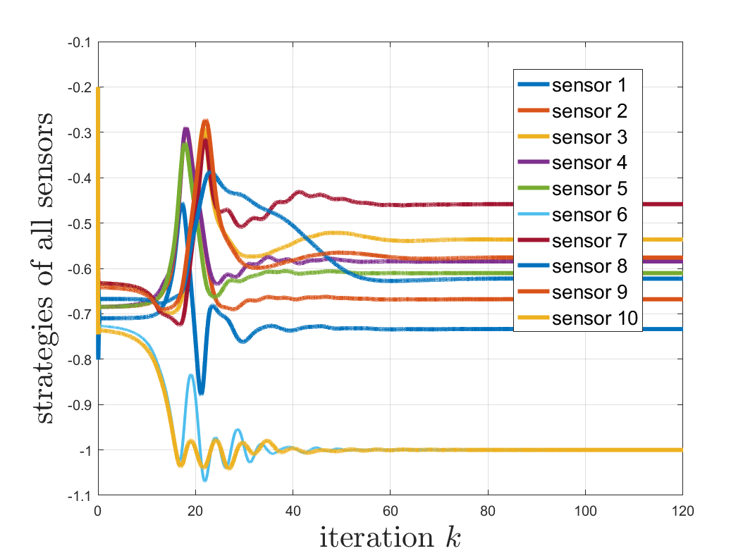
Figure 1: Convergence of all non-anchor nodes’ decisions

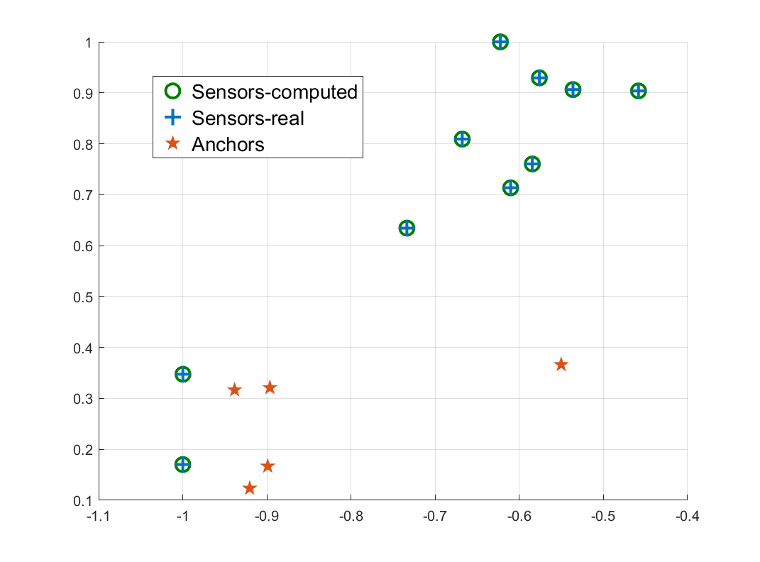
(a) $N=10$

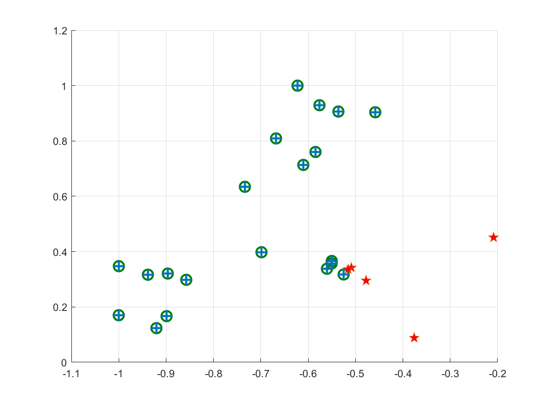
(b) $N=20$

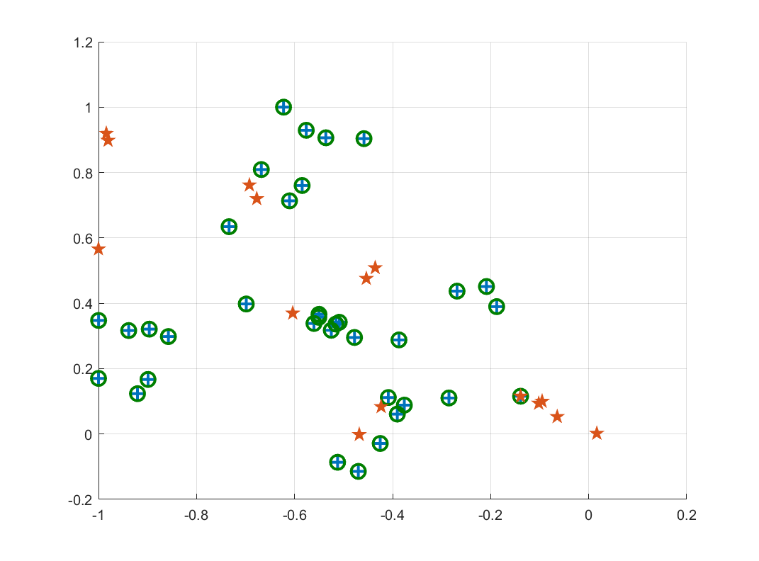
(c) $N=35$

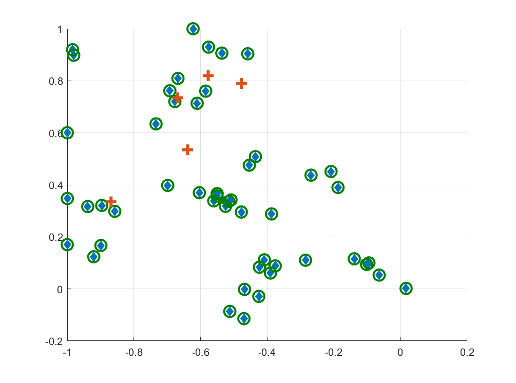
(d) $N=50$

Figure 2: Computed sensor location results with different configurations.

We first consider a two-dimensional case based on the UJIIndoorLoc dataset. The UJIIndoorLoc dataset was introduced in 2014 at the International Conference on Indoor Positioning and Indoor Navigation, which estimates user location based on building and floor. The dataset is available on the UC Irvine Machine Learning Repository website [36]. We extract the latitude and longitude coordinates of part of the sensors and standardize the data by doing min-max normalization. We employ Algorithm 1 to solve this problem. Set the tolerance $t_{tol}=10^{-5}$ and the terminal criterion $\|\boldsymbol{x}[k+1]-\boldsymbol{x}[k]\|\leq t_{tol},\;\|{\tau}[k+1]-{\tau}[k+1]\|\leq t_{tol}.$

TABLE I: MLE of four methods with three initializations in three iterations.

Initialization	Iteration	Values of $\operatorname{MLE}$
		Alg. 1 (ours)	Alg-SDP [37]	Alg-ARMA [11]	Alg-RBR[13]
$x_{11}[0]=5$	5	2.5781	2.7839	3.8108	3.8028
	50	0.9440	2.1493	2.8007	2.7902
	500	0.0002	1.5621	1.1114	1.4677
$x_{11}[0]=-5$	5	7.9650	8.1795	5.2786	11.8006
	50	1.5621	4.8478	3.9916	3.3692
	200	0.0002	2.9352	2.7148	2.7900
$x_{11}[0]=-0.5$	5	4.1795	4.5695	3.5691	3.6195
	50	2.7465	3.9715	2.8426	2.8426
	200	0.0002	2.6960	2.7517	2.7517

We show the effectiveness of Algorithm 1 for SNL problems with different node configurations. Take $N=10$ and $M=5$. In Fig. 1, we show the trajectories of these ten non-anchor nodes’ strategies in Algorithm 1 with respect to one certain dimension. This reveals that each non-anchor node finds its appropriate localization on account of the convergence, which actually serves as the desired global NE. Moreover, consider the effectiveness of our approach under different sensor network sizes. Take $N=10,20,35,50$ and different numbers of anchor nodes. Fig. 2 shows the computed sensor location results in these cases. The anchor nodes and the true locations of non-anchor nodes are shown by red stars and blue asterisks, and the computed locations are shown by green circles. We can see that Algorithm 1 can localize all sensors in either small or large sensor network sizes.

For further illustration in this task, we compare Algorithm 1 with several existing methods for the SNL problem. These compared algorithms include SDP-based algorithm [37], ARMA-based algorithm [11], and random best response (RBR) algorithm [13]. The performance of these methods can be evaluated by the mean localization error:

$$\operatorname{MLE}=\frac{1}{N}\sqrt{\sum_{i=1}^{N}\|x_{i}-x_{i}^{\star}\|^{2}}.$$

Take $N=25$. We randomly generate three different initial points as three cases and record the value of $\operatorname{MLE}$ of several methods under $5$, $50$, $500$ iterations respectively to measure the accuracy of the computed locations. All results are listed in Table I. In the first case $x^{0}_{11}=5$, only Algorithm 1 locates the non-anchor nodes accurately, while others remain with some errors. The value of $\operatorname{MLE}$ decreases with the increase of iterations. Also, in the other two cases $x^{0}_{11}=-5$ and $x^{0}_{11}=-0.5$, the advantage of Algorithm 1 is displayed while the errors of other methods are increased. This is because Algorithm 1 is insusceptible wherever the initial point lies and can efficiently handle the non-convex structures of this problem.

V Conclusion

In this paper, we have focused on the non-convex SNL problems. We have presented novel results on the identification condition of the global solution and the position-seeking algorithms. By formulating a non-convex SNL potential game, we have shown that the global NE exists and is unique. Then based on the canonical duality theory, we have proposed a conjugation-based algorithm to compute the stationary point of a complementary dual problem, which actually induces the global NE if a duality relation can be checked. Finally, the computational efficiency of our algorithm has been illustrated by several experiments.

In the future, we may extend our current results to more complicated cases such as i) generalizing the algorithm to distributed situations, ii) generalizing the model to cases with measurement noise, and iii) exploring milder graph conditions.

Appendix A Proof of Proposition 1

Given that the non-anchor nodes’ payoff functions $J_{i}$ are continuously differentiable, it follows from [22] that the condition (3) in Definition 1 is equivalent to

$$\frac{\partial J_{i}(x_{i},\boldsymbol{x}_{-i})}{\partial x_{i}}=\frac{\partial P(x_{i},\boldsymbol{x}_{-i})}{\partial x_{i}},\quad\text{ for }i\in\{1,\dots,N\}.$$

By computing the partial derivatives of $J_{i}$ and $P$, respectively, we can verify that $G$ is a potential game. $\square$

Appendix B Proof of Lemma 1

Recall the formulation of the non-convex function $P$. If all the non-anchor nodes are localized accurately such that $\|x_{i}^{\star}-x_{j}^{\star}\|^{2}-d_{ij}^{2}=0$ for any $(i,j)\in\mathcal{E}$, then $P(\boldsymbol{x}^{\star})$ tends to be zero. Thus $\boldsymbol{x}^{\star}$ is the global minimum of $P$. Moreover, referring to [38, 39], Assumption 1 guarantees that the global minimum of $P$ is unique and corresponds to the actual position profile $\boldsymbol{x}^{\star}$.

On the other hand, referring to Proposition 1, a global NE is equal to a global minimum of the potential function $P$. Since the global minimal of $P$ corresponds to the unique localization $\boldsymbol{x}^{\star}$ of the WSN, we can yield the conclusion. $\square$

Appendix C Proof of Theorem 1

If there exists ${\tau}^{\star}\in\Xi^{*}$ such that $(\boldsymbol{x}^{\star},\tau^{\star})$ is a stationary point of $\Psi(\boldsymbol{x},\tau)$, then it satisfies the first-order condition, that is

$$\mathbf{0}_{nN}\in\nabla_{\boldsymbol{x}}\,\tau^{\star\operatorname{T}}\Lambda\left(\boldsymbol{x}^{\star}\right)+\mathcal{N}_{\boldsymbol{\Omega}}(\boldsymbol{x}^{\star}),$$ (12a)

$$\mathbf{0}_{q}\in-\Lambda(\boldsymbol{x}^{\star})+\nabla\Phi^{*}(\tau^{\star})+\mathcal{N}_{\Xi^{*}}(\tau^{\star}),$$ (12b)

Moreover, based on the invertible one-to-one duality relation (8), for given $\xi\in\Xi$ with $\xi=\Lambda(\boldsymbol{x}^{\star})$, we have

$$\tau_{ij}^{\star}=\nabla_{\xi_{ij}}\Phi({\xi})|_{\xi_{ij}=\|x_{i}^{\star}-x_{j}^{\star}\|^{2}}\Leftrightarrow\xi_{ij}=\nabla\Phi^{*}(\tau_{ij}^{\star})$$

for $(i,j)\in\mathcal{E}$. By employing this relation in (12b), we have

$$\mathbf{0}_{q}=-\Lambda(\boldsymbol{x}^{\star})+\nabla\Phi^{*}(\tau^{\star}),$$

which implies

$$\tau^{\star}=\nabla\Phi(\Lambda(\boldsymbol{x}^{\star})).$$

By substituting $\tau^{\star}$ with $\nabla\Phi(\Lambda(\boldsymbol{x}^{\star}))$, we have

$$\mathbf{0}_{nN}\in\nabla_{\boldsymbol{x}}\,\Phi(\Lambda(\boldsymbol{x}^{\star}))^{\operatorname{T}}\Lambda\left(\boldsymbol{x}^{\star}\right)+\mathcal{N}_{\boldsymbol{\Omega}}(\boldsymbol{x}^{\star}).$$ (13)

According to the chain rule, $\nabla\Phi(\Lambda(\boldsymbol{x}^{\star}))^{\operatorname{T}}\Lambda\left(\boldsymbol{x}^{\star}\right)=\nabla_{\boldsymbol{x}}\Phi(\boldsymbol{x}^{\star}).$ Therefore, (13) is equivalent to

$$\mathbf{0}_{nN}\in\nabla_{\boldsymbol{x}}\Phi(\boldsymbol{x}^{\star})+\mathcal{N}_{\boldsymbol{\Omega}}(\boldsymbol{x}^{\star}).$$ (14)

According to the definition of potential game, (14) implies

$$\mathbf{0}_{n}\in\nabla_{x_{i}}J_{i}(x_{i}^{\star},\boldsymbol{x}_{-i}^{\star})+\mathcal{N}_{\Omega_{i}}({x_{i}^{\star}}),$$ (15)

which yields the conclusion. $\square$

Appendix D Proof of Theorem 2

If there exists ${\tau}^{\star}\in\mathbb{E}^{+}$ such that the pair $(\boldsymbol{x}^{\star},\tau^{\star})$ is a stationary point of Algorithm 1, then it satisfies the first-order condition with respect to $\Psi(x_{i},\boldsymbol{x}_{-i},\tau)$, that is

$$\mathbf{0}_{nN}\in\nabla_{\boldsymbol{x}}\,\tau^{\star\operatorname{T}}\Lambda\left(\boldsymbol{x}^{\star}\right)+\mathcal{N}_{\boldsymbol{\Omega}}(\boldsymbol{x}^{\star}),$$ (16a)

$$\mathbf{0}_{q}\in-\Lambda(\boldsymbol{x}^{\star})+\nabla\Phi^{*}(\tau^{\star})+\mathcal{N}_{\mathbb{E}^{+}}(\tau^{\star}),$$ (16b)

Together with $\tau_{ij}^{\star}=\nabla_{\xi_{ij}}\Phi({\xi})|_{\xi_{ij}=\|x_{i}^{\star}-x_{j}^{\star}\|^{2}},\forall(i,j)\in\mathcal{E}$, we claim that the canonical duality relation holds over $\boldsymbol{\Omega}\times\mathbb{E}^{+}$. Thus, (16b) becomes

$$\mathbf{0}_{q}=-\Lambda(\boldsymbol{x}^{\star})+\nabla\Phi^{*}(\tau^{\star}).$$

This indicates that the stationary point $(\boldsymbol{x}^{\star},{\tau^{\star}})$ of $\Psi(x_{i},\boldsymbol{x}_{-i},\tau)$ on $\boldsymbol{\Omega}\times\mathbb{E}^{+}$ is also a stationary point profile of $\Psi$ on $\boldsymbol{\Omega}\times\Xi^{*}$. Based on Theorem 1, we can further derive that the profile $\boldsymbol{x}^{\star}$ with respect to the stationary point $(\boldsymbol{x}^{\star},{\tau^{\star}})$ of $\Psi$ on $\boldsymbol{\Omega}\times\mathbb{E}^{+}$ is a Nash stationary point of game (1).

Moreover, recall

$$\mathbb{E}^{+}=\Xi^{*}\cap\{\tau:Q(\tau)\succeq\boldsymbol{0}_{nN}\}$$

with $Q(\tau)=\nabla^{2}_{\boldsymbol{x}}\Psi$. This indicates that $\Psi(\boldsymbol{x},\tau)$ is convex in $\boldsymbol{x}$. Also, note that $\Psi(\boldsymbol{x},\tau)$ is concave in dual variable $\tau$ due to the convexity of $\Phi(\cdot)$.

Thus, we can obtain the globally optimality of $(\boldsymbol{x}^{\star},\boldsymbol{\tau}^{\star})$ on $\boldsymbol{\Omega}\times\mathbb{E}^{+}$, that is, for $\boldsymbol{x}\in\boldsymbol{\Omega}$ and $\tau\in\mathbb{E}^{+}$,

$$\Psi(\boldsymbol{x}^{\star},\tau)\leq\Psi(\boldsymbol{x}^{\star},\tau^{\star})\leq\Psi(\boldsymbol{x},\tau^{\star}).$$

The inequality relation above tells that

$$J_{i}(x_{i}^{\star},\boldsymbol{x}_{-i}^{\star})\leq J_{i}(x_{i},\boldsymbol{x}_{-i}^{\star}),\quad\forall x_{i}\in\Omega_{i},\quad\forall i\in\mathcal{N}_{s}.$$

This confirms that $\boldsymbol{x}^{\star}$ is the global NE of (1), which completes the proof. $\square$

References

- [1] I. F. Akyildiz, W. Su, Y. Sankarasubramaniam, and E. Cayirci, “Wireless sensor networks: a survey,” Computer Networks, vol. 38, no. 4, pp. 393–422, 2002.
- [2] Q. Liu, Z. Wang, X. He, and D.-H. Zhou, “Event-based recursive distributed filtering over wireless sensor networks,” IEEE Transactions on Automatic Control, vol. 60, no. 9, pp. 2470–2475, 2015.
- [3] N. Marechal, J.-M. Gorce, and J.-B. Pierrot, “Joint estimation and gossip averaging for sensor network applications,” IEEE Transactions on Automatic Control, vol. 55, no. 5, pp. 1208–1213, 2010.
- [4] G. Jing, C. Wan, and R. Dai, “Angle-based sensor network localization,” IEEE Transactions on Automatic Control, vol. 67, no. 2, pp. 840–855, 2021.
- [5] G. Sun, G. Qiao, and B. Xu, “Corrosion monitoring sensor networks with energy harvesting,” IEEE Sensors Journal, vol. 11, no. 6, pp. 1476–1477, 2010.
- [6] T. Sun, L.-J. Chen, C.-C. Han, and M. Gerla, “Reliable sensor networks for planet exploration,” in Proceedings. 2005 IEEE Networking, Sensing and Control, 2005. IEEE, 2005, pp. 816–821.
- [7] G. Jing, G. Zhang, H. W. Joseph Lee, and L. Wang, “Weak rigidity theory and its application to formation stabilization,” SIAM Journal on Control and optimization, vol. 56, no. 3, pp. 2248–2273, 2018.
- [8] D. Estrin, R. Govindan, and J. Heidemann, “Embedding the internet: introduction,” Communications of the ACM, vol. 43, no. 5, pp. 38–41, 2000.
- [9] A. Savvides, C.-C. Han, and M. B. Strivastava, “Dynamic fine-grained localization in ad-hoc networks of sensors,” in Proceedings of the 7th annual international conference on Mobile computing and networking, 2001, pp. 166–179.
- [10] G. Mao, B. Fidan, and B. D. Anderson, “Wireless sensor network localization techniques,” Computer Networks, vol. 51, no. 10, pp. 2529–2553, 2007.
- [11] C. Wan, G. Jing, S. You, and R. Dai, “Sensor network localization via alternating rank minimization algorithms,” IEEE Transactions on Control of Network Systems, vol. 7, no. 2, pp. 1040–1051, 2019.
- [12] S. P. Ahmadi, A. Hansson, and S. K. Pakazad, “Distributed localization using levenberg-marquardt algorithm,” EURASIP Journal on Advances in Signal Processing, vol. 2021, no. 1, pp. 1–26, 2021.
- [13] J. Jia, G. Zhang, X. Wang, and J. Chen, “On distributed localization for road sensor networks: A game theoretic approach,” Mathematical Problems in Engineering, vol. 2013, 2013.
- [14] B. Bejar, P. Belanovic, and S. Zazo, “Cooperative localisation in wireless sensor networks using coalitional game theory,” in 2010 18th European Signal Processing Conference. IEEE, 2010, pp. 1459–1463.
- [15] G. Chen, G. Xu, F. He, Y. Hong, L. Rutkowski, and D. Tao, “Global nash equilibrium in non-convex multi-player game: Theory and algorithms,” arXiv preprint arXiv:2301.08015, 2023.
- [16] J. Nash, “Non-cooperative games,” Annals of Mathematics, pp. 286–295, 1951.
- [17] G. Xu, G. Chen, H. Qi, and Y. Hong, “Efficient algorithm for approximating Nash equilibrium of distributed aggregative games,” IEEE Transactions on Cybernetics, 2022.
- [18] M. Ke, Y. Xu, A. Anpalagan, D. Liu, and Y. Zhang, “Distributed TOA-based positioning in wireless sensor networks: A potential game approach,” IEEE Communications Letters, vol. 22, no. 2, pp. 316–319, 2017.
- [19] Z. Wang, S. Zheng, S. Boyd, and Y. Ye, “Further relaxations of the SDP approach to sensor network localization,” Tech. Rep., 2006.
- [20] P. Tseng, “Second-order cone programming relaxation of sensor network localization,” SIAM Journal on Optimization, vol. 18, no. 1, pp. 156–185, 2007.
- [21] J. R. Marden, G. Arslan, and J. S. Shamma, “Cooperative control and potential games,” IEEE Transactions on Systems, Man, and Cybernetics, Part B (Cybernetics), vol. 39, no. 6, pp. 1393–1407, 2009.
- [22] D. Monderer and L. S. Shapley, “Potential games,” Games and Economic Behavior, vol. 14, no. 1, pp. 124–143, 1996.
- [23] M. Nouiehed, M. Sanjabi, T. Huang, J. D. Lee, and M. Razaviyayn, “Solving a class of non-convex min-max games using iterative first order methods,” Advances in Neural Information Processing Systems, vol. 32, 2019.
- [24] M. Heusel, H. Ramsauer, T. Unterthiner, B. Nessler, and S. Hochreiter, “Gans trained by a two time-scale update rule converge to a local Nash equilibrium,” Advances in Neural Information Processing Systems, vol. 30, 2017.
- [25] B. D. Anderson, I. Shames, G. Mao, and B. Fidan, “Formal theory of noisy sensor network localization,” SIAM Journal on Discrete Mathematics, vol. 24, no. 2, pp. 684–698, 2010.
- [26] B. Fidan, J. M. Hendrickx, and B. D. Anderson, “Closing ranks in rigid multi-agent formations using edge contraction,” International Journal of Robust and Nonlinear Control, vol. 20, no. 18, pp. 2077–2092, 2010.
- [27] T.-S. Tay and W. Whiteley, “Generating isostatic frameworks,” Structural Topology 1985 Núm 11, 1985.
- [28] G. Chen, Y. Ming, Y. Hong, and P. Yi, “Distributed algorithm for -generalized Nash equilibria with uncertain coupled constraints,” Automatica, vol. 123, p. 109313, 2021.
- [29] G. C. Calafiore, L. Carlone, and M. Wei, “Distributed optimization techniques for range localization in networked systems,” in 49th IEEE Conference on Decision and Control (CDC). IEEE, 2010, pp. 2221–2226.
- [30] Q. Shi, C. He, H. Chen, and L. Jiang, “Distributed wireless sensor network localization via sequential greedy optimization algorithm,” IEEE Transactions on Signal Processing, vol. 58, no. 6, pp. 3328–3340, 2010.
- [31] B. D. Anderson, C. Yu, B. Fidan, and J. M. Hendrickx, “Rigid graph control architectures for autonomous formations,” IEEE Control Systems Magazine, vol. 28, no. 6, pp. 48–63, 2008.
- [32] K. Cao, Z. Han, Z. Lin, and L. Xie, “Bearing-only distributed localization: A unified barycentric approach,” Automatica, vol. 133, p. 109834, 2021.
- [33] F. Facchinei and C. Kanzow, “Penalty methods for the solution of generalized Nash equilibrium problems,” SIAM Journal on Optimization, vol. 20, no. 5, pp. 2228–2253, 2010.
- [34] J. Koshal, A. Nedić, and U. V. Shanbhag, “Distributed algorithms for aggregative games on graphs,” Operations Research, vol. 64, no. 3, pp. 680–704, 2016.
- [35] D. Y. Gao, V. Latorre, and N. Ruan, Canonical Duality Theory: Unified Methodology for Multidisciplinary Study. Springer, 2017.
-
[36]
D. Dua and C. Graff,
http://archive.ics.uci.edu/dataset/343/ujiindoorloc+m
ag, Accessed on 2019. - [37] K. W. K. Lui, W.-K. Ma, H.-C. So, and F. K. W. Chan, “Semi-definite programming algorithms for sensor network node localization with uncertainties in anchor positions and/or propagation speed,” IEEE Transactions on Signal Processing, vol. 57, no. 2, pp. 752–763, 2008.
- [38] T. Eren, O. Goldenberg, W. Whiteley, Y. R. Yang, A. S. Morse, B. D. Anderson, and P. N. Belhumeur, “Rigidity, computation, and randomization in network localization,” in IEEE INFOCOM 2004, vol. 4. IEEE, 2004, pp. 2673–2684.
- [39] J. Aspnes, T. Eren, D. K. Goldenberg, A. S. Morse, W. Whiteley, Y. R. Yang, B. D. Anderson, and P. N. Belhumeur, “A theory of network localization,” IEEE Transactions on Mobile Computing, vol. 5, no. 12, pp. 1663–1678, 2006.