The chiral condensate at large $N$

Abstract

We present results for the large-$N$ limit of the chiral condensate computed from twisted reduced models. We followed a two-fold strategy, one constiting in extracting the condensate from the quark-mass dependence of the pion mass, the other consisting in extracting the condensate from the mode number of the Dirac operator.

1 Introduction

Lattice strategies to study the large-$N$ limit of gauge theories can be mainly divided into two broad classes:

• Standard approaches, namely, numerical results obtained from theories discretized on regular extended lattices for $N\lesssim 10$ are extrapolated towards $1/N\to 0$ [1, 2, 3, 4, 5, 6, 7, 8, 9, 10, 11];

• Reduced models [12, 13, 14, 15], namely, calculations are performed for $N=O(100)$ or larger (i.e., practically already in the large-$N$ limit), with the lattice volume either very small or completely reduced to just a single point [16, 18, 19, 20, 21, 22, 23, 24, 25, 26, 27, 28, 29].

These two different methods can be regarded as complementary. On one hand, the excellent agreement found for the large-$N$ limit of several observables obtained from these two different methods is highly non-trivial. On the other hand, since the finite-$N$ corrections of the reduced models are different from those of the standard approach, results from both methods can be combined to extract the actual $N$-dependence of a given observable.

This manuscript deals with the computation of the large-$N$ limit of an observable which plays an intriguing role both from the theoretical and the phenomenological point of view: the chiral condensate. The computation of this observable has been performed for $\mathrm{SU}(3)$ with a variety of lattice discretizations and fermion contents [30, 31, 32, 33, 34, 35, 36, 37], but so far only few large-$N$ determinations have been given in the literature, either involving just one lattice spacing [38, 6], or presenting a preliminary study of the large-$N$ limit [11]. This proceeding reports on the main results of [39], where the large-$N$ limit of the chiral condensate is computed using the Twisted Eguchi–Kawai (TEK) model [14, 15]. In particular, we obtain the chiral condensate at large $N$ from the low-lying spectrum of the Dirac operator, and we perform controlled continuum and chiral extrapolations to provide a solid determination of this quantity in the large-$N$ limit. Perfectly compatible results are obtained from the quark mass dependence of the pion mass, as we will show in the following.

This paper is organized as follows: in Sec. 2 we briefly summarize our numerical setup; in Sec. 3 we present and discuss the main results of [39] about the large-$N$ limit of the chiral condensate; finally in Sec. 4 we draw our conclusions.

2 Numerical setup

Below we briefly summarize our TEK lattice discretization, as well as the Giusti–Lüscher method to extract the chiral condensate from the low-lying spectrum of the lattice Dirac–Wilson operator.

2.1 Lattice discretization

The pure-gauge TEK model is a matrix model where the dynamical degrees of freedom are $d=4$ $\mathrm{SU}(N)$ matrices. It can be thought of as the reduction on a single site lattice of an ordinary Wilson lattice Yang–Mills theory defined on a discretized torus with twisted periodic boundary conditions. The Wilson pure-gauge TEK action reads:

$$S_{\mathrm{W}}^{(\mathrm{TEK})}[U]=-Nb\sum_{\nu\neq\mu}z_{\nu\mu}\mathrm{Tr}\left\{U_{\mu}U_{\nu}U_{\mu}^{\dagger}U_{\nu}^{\dagger}\right\},$$ (1)

where $1/b$ is the bare ’t Hooft coupling, $U_{\mu}$ are the $\mathrm{SU}(N)$ $d=4$ link matrices, $N=L^{2}$, and $z_{\nu\mu}=z_{\mu\nu}^{*}=\exp\left\{i\frac{2\pi k(N)}{\sqrt{N}}\right\}$ ($\nu>\mu$) is the twist factor, with $k(N)$ an integer number co-prime with $\sqrt{N}\in\mathbb{Z}$. There is now plenty of theoretical and numerical evidence that this model reproduces the infinite-volume large-$N$ behavior of ordinary Yang–Mills gauge theories [18, 24, 20, 21, 25, 27]. Concerning Monte Carlo methods, gauge configurations were generated using the over-relaxation algorithm described in [23].

In our work we do not consider any dynamical fermion, as in the large-$N$ limit the contributions of fundamental flavors is exactly zero. We will however consider one flavor of Dirac–Wilson fermions in the valence sector. In this case the lattice Dirac operator reads [24]:

$$D_{\mathrm{W}}^{(\mathrm{TEK})}[U]=\frac{1}{2\kappa}-\frac{1}{2}\sum_{\mu}\left[(\mathbb{I}+\gamma_{\mu})\otimes\mathcal{W}_{\mu}[U]+(\mathbb{I}-\gamma_{\mu})\otimes\mathcal{W}_{\mu}^{\dagger}\right],$$ (2)

with $\kappa$ the hopping parameter and $\mathcal{W}_{\mu}[U]\equiv U_{\mu}\otimes\Gamma_{\mu}^{*}$, where $\Gamma_{\mu}$ represent the twist eaters, satisfying $\Gamma_{\mu}\Gamma_{\nu}=z_{\nu\mu}^{*}\Gamma_{\nu}\Gamma_{\mu}$.

2.2 The Giusti–Lüscher method

The Banks–Casher relation equates the chiral condensate to the spectral density $\rho$ of the eigenmodes of the Dirac operator in the origin:

$$\frac{\Sigma}{\pi}=\lim_{\lambda\to 0}\lim_{m\to 0}\lim_{V\to\infty}\rho(\lambda,m)$$ (3)

Another physical quantity that is equivalent to $\rho$, but that is more convenient to be computed on the lattice, is the mode number of the massive Dirac operator:

$$\braket{\nu(M)} \equiv \braket{\#\,\,}{i\lambda+m}{\leq M}$$ (4)

$$= V\int_{-\Lambda}^{\Lambda}\rho(\lambda,m)d\lambda,\qquad\Lambda^{2}\equiv M^{2}-m^{2}.$$ (5)

Being the mode number and the spectral density connected by an integral relation, it is clear that the Banks–Casher implies a linear behavior of $\braket{\nu(M)}$ as a function of $\Lambda$:

$$\braket{\nu(M)}=\frac{2}{\pi}V\Sigma\Lambda+o(\Lambda),$$ (6)

where higher-order terms in $\Lambda$ are sub-leading in $1/N$ [40, 41].

The Giusti–Lüscher method [42] consists in obtaining the chiral condensate $\Sigma$ from a numerical lattice computation of the slope of the mode number of the Dirac operator as:

$$\Sigma^{(\mathrm{eff})}(m) = \frac{\pi}{2V}\sqrt{1-\left(\frac{m}{\overline{M}}\right)^{2}}\left[\frac{\partial\braket{\nu(M)}}{\partial M}\right]\Bigg{|}_{M=\overline{M}}\longleftarrow\text{slope of $\braket{\nu(M)}$ in $M=\overline{M}$},$$ (7)

$$\Sigma = \lim_{m\to 0}\Sigma^{(\mathrm{eff})}(m),$$ (8)

where $\overline{M}$ is the point in which the slope is computed.

As a final comment, let us here stress that, within TEK models, the obtained results should be thought of as if they were obtained on a lattice with effective size $\ell=aL=a\sqrt{N}$. Therefore, the volume appearing in (7) is given by $V=a^{4}(\sqrt{N})^{4}=a^{4}N^{2}$.

3 Results

In this manuscript, we will mainly refer to results obtained for $N=289$, for which the $k$ parameter appearing in the twist factor defined in the previous section was chosen to be $k=5$. Since we expect the following large-$N$ scaling for the chiral condensate:

$$\Sigma(N)=N\left[\bar{\Sigma}+O\left(\frac{1}{N^{2}}\right)\right],$$ (9)

in the following we will always report results for $\Sigma/N$, which we expect to approach a finite large-$N$ limit. Finally, all reported results for the renormalized chiral condensate are always expressed in the $\overline{\mathrm{MS}}$ scheme at the conventional renormalization scale $\mu=2~{}\mathrm{GeV}$.

3.1 Best fit of the mode number

Let us summarize our practical numerical implementation of the Giusti–Lüscher method, as well as the procedure we followed to compute the chiral condensate from our Dirac spectra:

• Renormalization properties: $\braket{\nu}=\braket{\nu_{\mathrm{R}}}$, $\quad M_{\mathrm{R}}=M/Z_{\mathrm{P}}$, $\quad\lambda_{\mathrm{R}}=\lambda/Z_{\mathrm{P}}$;

• Scale setting: determinations of the string tension $a\sqrt{\sigma}$ obtained from the TEK model in Refs. [18, 27];

• We solved numerically the eigenproblem $(\gamma_{5}D^{(\mathrm{TEK})}_{\mathrm{W}}[U])u_{\lambda}=\lambda u_{\lambda}$ for 100 well-decorrelated gauge configurations using the ARPACK library, and computed the first 300 lowest-lying eigenvalues and eigenvectors;

• From the knowledge of $Z_{\mathrm{A}}$ and $m_{\mathrm{PCAC}}$ (computed at large-$N$ from the TEK model in Ref. [27]), we obtained the renormalized eigenvalues as: $\lambda_{\mathrm{R}}/m_{\mathrm{R}}=\lambda/(Z_{\mathrm{A}}m_{\mathrm{PCAC}})$;

• We counted the renormalized modes $\lambda_{\mathrm{R}}/m_{\mathrm{R}}$ below the threshold $M_{\mathrm{R}}/m_{\mathrm{R}}$ to obtain $\braket{\nu(M_{\mathrm{R}})}=\braket{\nu_{\mathrm{R}}(M_{\mathrm{R}})}$;

• From a linear best fit of $\braket{\nu_{\mathrm{R}}(M_{\mathrm{R}})}/N$ vs $M_{\mathrm{R}}/m_{\mathrm{R}}$ we obtain the slope $\left[\frac{\partial\braket{\nu(M)}}{\partial M}\right]\Big{|}_{M=\overline{M}}$, where $\overline{M}$ is the middle point of the fit range (cf. Fig. 1, top panel);

• From the slope of the mode number we extract the RG-invariant quantity $\Sigma^{(\mathrm{eff})}_{\mathrm{R}}m_{\mathrm{R}}/(\sigma^{2}N)$ from Eq. (7);

• Using $Z_{\mathrm{A}}m_{\mathrm{PCAC}}=Z_{\mathrm{P}}m_{\mathrm{R}}$ and the conventional value $\sqrt{\sigma}=440$ MeV, we get rid of the quark mass and finally obtain the bare effective chiral condensate $\Sigma^{(\mathrm{eff})}_{\mathrm{R}}/(\sigma^{3/2}NZ_{\mathrm{P}})$ in MeV³;

• All our results where obtained for $N=289$, but we explicitly checked that results obtained for $N=361$ gave perfectly agreeing results (cf. Fig. 1, bottom panel).

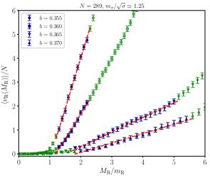
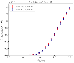
Figure 1: Linear best fit of the mode number $\braket{\nu_{\mathrm{R}}}/N$ as a function of $M_{\mathrm{R}}/m_{\mathrm{R}}$ for 4 different values of the ’t Hooft coupling $1/b$, and for 4 different values of $\kappa$ tuned to correspond approximately to the same value of the pion mass $m_{\pi}$ (top plot). Filled points correspond to the fitted ones. All our results refer to $N=289$, but in one case (bottom plot) we also checked that results obtained for $N=361$ where perfectly agreeing (in the latter case, $k=7$ was used for the twist factor).

3.2 Chiral limit at fixed lattice spacing

After obtaining the bare effective chiral condensate from the Giusti–Lüscher method, we need to extrapolate our determinations towards the chiral limit, in order to get rid of the finite quark mass we have used to determine our Dirac spectra. Our extrapolations towards the chiral limit, shown in Fig. 2, are done according to the Chiral Perturbation Theory (ChPT) prediction:

$$\Sigma^{(\mathrm{eff})}(m) = \Sigma+k\,m+o(m)$$ (10)

$$= \Sigma+k^{\prime}\,m_{\pi}^{2}+o(m_{\pi}^{2}),$$ (11)

with $\Sigma^{(\mathrm{eff})}=\Sigma^{(\mathrm{eff})}_{\mathrm{R}}/Z_{\mathrm{P}}$. Our chiral extrapolations will be performed, in all cases, at fixed $b$, i.e., at fixed lattice spacing. Thus, the renormalization constant $Z_{\mathrm{P}}$ will be, at fixed $b$, the same for all explored values of the pion mass $m_{\pi}$.

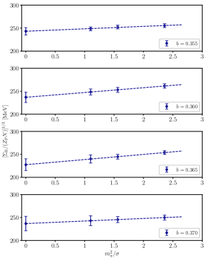
Figure 2: Extrapolation towards the chiral limit of the bare effective chiral condensate $[\Sigma^{(\mathrm{eff})}_{\mathrm{R}}/(NZ_{\mathrm{P}})]^{1/3}$ expressed in MeV physical units for all explored values of the ’t Hooft coupling.

3.3 Continuum limit

In order to extrapolate our results towards the chiral limit, we renormalize our large-$N$ determinations of $\Sigma_{\mathrm{R}}$ using the large-$N$ non-perturbative determinations of $Z_{\mathrm{P}}$ reported in [43], where we refer the reader for more details about the numerical techniques to compute this renormalization constant from lattice simulations.

The continuum extrapolation of our spectral determinations of the chiral condensate, shown in Fig. 3 (top panel), are done assuming leading $O(a^{2})$ corrections as usual:

$$\Sigma_{\mathrm{R}}(a)=\Sigma_{\mathrm{R}}+c\,a^{2}+o(a^{2}).$$ (12)

In the top panel of Fig. 3 we also show the renormalized determinations of the chiral condensate obtained from the Gell-Man–Oakes–Renner (GMOR) relation,

$$m_{\pi}^{2}=2\frac{\Sigma}{F_{\pi}^{2}}m=2\frac{\Sigma_{\mathrm{R}}}{F_{\pi}^{2}}m_{\mathrm{R}},$$ (13)

according to the large-$N$ TEK determinations of the pion mass and of the pion decay constant of Ref. [27]. We find perfectly agreeing results once the continuum limit is taken. Thus, we perform a combined continuum limit (see bottom panel of Fig. 3), giving the joint estimate:

$$(\Sigma_{\mathrm{R}}/N)^{1/3}=184(13)~{}\mathrm{MeV}.$$ (14)

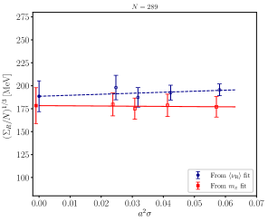
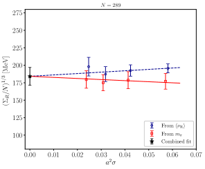
Figure 3: Extrapolation towards the chiral limit of the spectral determinations of the chiral condensate obtained from the Giusti–Lüscher method, compared with the determinations obtained from the GMOR relation (13) and using the determinations of $m_{\pi}$ vs $m$ and of $F_{\pi}$ of Ref. [27]. In the top panel we show individual fits of the two data sets, in the bottom panel we show instead the combined fit of the two data sets.

4 Conclusions

This manuscript reports on the main results of Ref. [39], which presents a solid computation of the large-$N$ chiral condensate from TEK models using the Giusti–Lüscher spectral method for $N=289$, using 4 lattice spacings and 3 pion masses each to provide controlled chiral and continuum extrapolations. The obtained results are in perfect agreement with those obtained from the quark mass dependence of the pion mass and the GMOR relation, giving a joint estimate of:

$$\lim_{N\to\infty}\frac{\Sigma_{\mathrm{R}}(N)}{N}=[184(13)\text{ MeV}]^{3},\qquad\text{ ($\overline{\mathrm{MS}}$, $\,\,\mu=2~{}\mathrm{GeV}$, $\,\,\sqrt{\sigma}=440$ MeV)}$$ (15)

Our final result is in remarkable agreement with the FLAG21 [44] world-average for 2-flavor QCD $\Sigma_{\mathrm{R}}(N=3)/3=[184(7)\text{ MeV}]^{3}$ when using $\sqrt{\sigma}$ to set the scale. Our calculation thus points out that $1/N^{2}$ corrections are small and $N=3$ is already very close to $N=\infty$. Such conclusion fits very well with other large-$N$ calculations pointing towards the same scenario [1, 2, 3, 4, 6, 7, 8, 9, 10].

In the next future, we plan to extend our calculation of the chiral condensate to the case of adjoint Majorana fermions, which is of great theoretical interest.

References

- [1] B. Lucini and M. Panero, SU() gauge theories at large , Phys. Rept. 526 (2013) 93 [1210.4997].
- [2] G. S. Bali, F. Bursa, L. Castagnini, S. Collins, L. Del Debbio, B. Lucini et al., Mesons in large-N QCD, JHEP 06 (2013) 071 [1304.4437].
- [3] C. Bonati, M. D’Elia, P. Rossi and E. Vicari, dependence of 4D gauge theories in the large- limit, Phys. Rev. D 94 (2016) 085017 [1607.06360].
- [4] M. Cè, M. Garcia Vera, L. Giusti and S. Schaefer, The topological susceptibility in the large- limit of SU() Yang-Mills theory, Phys. Lett. B 762 (2016) 232 [1607.05939].
- [5] T. DeGrand and Y. Liu, Lattice study of large QCD, Phys. Rev. D 94 (2016) 034506 [1606.01277].
- [6] P. Hernández, C. Pena and F. Romero-López, Large scaling of meson masses and decay constants, Eur. Phys. J. C 79 (2019) 865 [1907.11511].
- [7] E. Bennett, J. Holligan, D. K. Hong, J.-W. Lee, C. J. D. Lin, B. Lucini et al., Color dependence of tensor and scalar glueball masses in Yang-Mills theories, Phys. Rev. D 102 (2020) 011501 [2004.11063].
- [8] C. Bonanno, C. Bonati and M. D’Elia, Large- Yang-Mills theories with milder topological freezing, JHEP 03 (2021) 111 [2012.14000].
- [9] A. Athenodorou and M. Teper, SU(N) gauge theories in 3+1 dimensions: glueball spectrum, string tensions and topology, JHEP 12 (2021) 082 [2106.00364].
- [10] C. Bonanno, M. D’Elia, B. Lucini and D. Vadacchino, Towards glueball masses of large-N SU(N) pure-gauge theories without topological freezing, Phys. Lett. B 833 (2022) 137281 [2205.06190].
- [11] T. A. DeGrand and E. Wickenden, Lattice study of the chiral properties of large QCD, 2309.12270.
- [12] T. Eguchi and H. Kawai, Reduction of dynamical degrees of freedom in the large- gauge theory, Phys. Rev. Lett. 48 (1982) 1063.
- [13] G. Bhanot, U. M. Heller and H. Neuberger, The quenched Eguchi-Kawai model, Physics Letters B 113 (1982) 47.
- [14] A. Gonzalez-Arroyo and M. Okawa, A twisted model for large- lattice gauge theory, Physics Letters B 120 (1983) 174.
- [15] A. Gonzalez-Arroyo and M. Okawa, Twisted-eguchi-kawai model: A reduced model for large- lattice gauge theory, Phys. Rev. D 27 (1983) 2397.
- [16] A. Gonzalez-Arroyo and M. Okawa, Large reduction with the Twisted Eguchi-Kawai model, JHEP 07 (2010) 043 [1005.1981].
- [17] A. Hietanen and R. Narayanan, Numerical evidence for non-analytic behavior in the beta function of large N SU(N) gauge theory coupled to an adjoint Dirac fermion, Phys. Rev. D 86 (2012) 085002 [1204.0331].
- [18] A. Gonzalez-Arroyo and M. Okawa, The string tension from smeared Wilson loops at large N, Phys. Lett. B 718 (2013) 1524 [1206.0049].
- [19] R. Lohmayer and R. Narayanan, Weak-coupling analysis of the single-site large- gauge theory coupled to adjoint fermions, Phys. Rev. D 87 (2013) 125024 [1305.1279].
- [20] A. Gonzalez-Arroyo and M. Okawa, Testing volume independence of SU(N) pure gauge theories at large N, JHEP 12 (2014) 106 [1410.6405].
- [21] M. García Pérez, A. González-Arroyo, L. Keegan and M. Okawa, The twisted gradient flow running coupling, JHEP 01 (2015) 038 [1412.0941].
- [22] M. García Pérez, A. González-Arroyo, L. Keegan and M. Okawa, Mass anomalous dimension of Adjoint QCD at large N from twisted volume reduction, JHEP 08 (2015) 034 [1506.06536].
- [23] M. García Pérez, A. González-Arroyo, L. Keegan, M. Okawa and A. Ramos, A comparison of updating algorithms for large N reduced models, JHEP 06 (2015) 193 [1505.05784].
- [24] A. González-Arroyo and M. Okawa, Large N meson masses from a matrix model, Phys. Lett. B 755 (2016) 132 [1510.05428].
- [25] M. García Pérez, A. González-Arroyo and M. Okawa, Perturbative contributions to Wilson loops in twisted lattice boxes and reduced models, JHEP 10 (2017) 150 [1708.00841].
- [26] M. García Pérez, Prospects for large N gauge theories on the lattice, PoS LATTICE2019 (2020) 276 [2001.10859].
- [27] M. García Pérez, A. González-Arroyo and M. Okawa, Meson spectrum in the large limit, JHEP 04 (2021) 230 [2011.13061].
- [28] P. Butti, M. García Pérez, A. Gonzalez-Arroyo, K.-I. Ishikawa and M. Okawa, Scale setting for large-N SUSY Yang-Mills on the lattice, JHEP 07 (2022) 074 [2205.03166].
- [29] P. Butti and A. Gonzalez-Arroyo, Asymptotic scaling in Yang-Mills theory at large-, PoS LATTICE2023 (2023) 381.
- [30] G. P. Engel, L. Giusti, S. Lottini and R. Sommer, Spectral density of the Dirac operator in two-flavor QCD, Phys. Rev. D 91 (2015) 054505 [1411.6386].
- [31] P. A. Boyle et al., Low energy constants of SU(2) partially quenched chiral perturbation theory from Nf=2+1 domain wall QCD, Phys. Rev. D 93 (2016) 054502 [1511.01950].
- [32] C. Wang, Y. Bi, H. Cai, Y. Chen, M. Gong and Z. Liu, Quark chiral condensate from the overlap quark propagator, Chin. Phys. C 41 (2017) 053102 [1612.04579].
- [33] C. Alexandrou, A. Athenodorou, K. Cichy, M. Constantinou, D. P. Horkel, K. Jansen et al., Topological susceptibility from twisted mass fermions using spectral projectors and the gradient flow, Phys. Rev. D 97 (2018) 074503 [1709.06596].
- [34] JLQCD collaboration, S. Aoki, G. Cossu, H. Fukaya, S. Hashimoto and T. Kaneko, Topological susceptibility of QCD with dynamical Möbius domain-wall fermions, PTEP 2018 (2018) 043B07 [1705.10906].
- [35] Extended Twisted Mass collaboration, C. Alexandrou et al., Quark masses using twisted-mass fermion gauge ensembles, Phys. Rev. D 104 (2021) 074515 [2104.13408].
- [36] J. Liang, A. Alexandru, Y.-J. Bi, T. Draper, K.-F. Liu and Y.-B. Yang, Detecting flavor content of the vacuum using the Dirac operator spectrum, 2102.05380.
- [37] C. Bonanno, F. D’Angelo and M. D’Elia, The chiral condensate of QCD from the spectrum of the staggered Dirac operator, 2308.01303.
- [38] R. Narayanan and H. Neuberger, Chiral symmetry breaking at large , Nucl. Phys. B 696 (2004) 107 [hep-lat/0405025].
- [39] C. Bonanno, P. Butti, M. García Peréz, A. González-Arroyo, K.-I. Ishikawa and M. Okawa, The large- limit of the chiral condensate from twisted reduced models, 2309.15540.
- [40] A. Smilga and J. Stern, On the spectral density of euclidean dirac operator in qcd, Physics Letters B 318 (1993) 531.
- [41] J. C. Osborn, D. Toublan and J. J. M. Verbaarschot, From chiral random matrix theory to chiral perturbation theory, Nucl. Phys. B 540 (1999) 317 [hep-th/9806110].
- [42] L. Giusti and M. Lüscher, Chiral symmetry breaking and the Banks-Casher relation in lattice QCD with Wilson quarks, JHEP 03 (2009) 013 [0812.3638].
- [43] L. Castagnini, Meson spectroscopy in Large- QCD, [inspirehep/1411974] (2015) .
- [44] Flavour Lattice Averaging Group (FLAG) collaboration, Y. Aoki et al., FLAG Review 2021, Eur. Phys. J. C 82 (2022) 869 [2111.09849].