Approximation Algorithms for Line Planning with Resource Constraints

Abstract

Our study aims to maximize the total reward in a transportation system with $M$ buses that serve specific Origin-Destination (OD) pairs. Each bus can operate on at most one line from a set of candidate lines. Operating a line incurs different types of resource costs. The goal is to efficiently assign the buses to the lines to serve integral portions of given OD demands while respecting bus capacity, resource limits, and demand constraints.

We propose a series of algorithms that address various facets of the problem. For a scenario where all lines costs are zero, we achieve an optimal approximation ratio of $1-\frac{1}{e}$, assuming $P\neq NP$. For instances with sufficiently small line costs, our algorithm reaches an approximation ratio of $1-\frac{1}{e}-\eta$. For the most general case, we obtain an approximation ratio of $\frac{1}{2}-\frac{1}{2e}-\eta$. Lastly, we offer an approach that ensures an approximation ratio of $1-\frac{1}{e}-\eta$ while limiting resource usage to at most $1+\tau$ units for each type of resource. Here $\eta$ and $\tau$ are arbitrary fixed constants.

Our results also extend current methods and provide new avenues for addressing a broad class of assignment problems involving multiple resource constraints.

1 The Problem

We consider a transportation system composed of $M$ buses operating in a transportation network. Each bus, labeled by $b$, has a set $\mathcal{L}_{b}$ of candidate lines on which it can operate. Each line can be viewed as a directed path (possibly closed). This system is designed to serve a collection $D$ of Origin-Destination (OD) pairs. Each OD pair $(i,j)$ has demand $d_{(i,j)}$ which can be interpreted as the number of people who need to go from location $i$ to location $j$ in a given time span. We can serve an integral portion of the demand $d_{(i,j)}$, denoted by $\xi_{b,l,(i,j)}\in\left[0,d_{(i,j)}\right]\cap\mathbb{Z}$, with bus $b$ operating on line $l$, provided that line $l$ goes through the locations $i$ and $j$ in the direction from $i$ to $j$. The associated reward is $v_{b,l,(i,j)}\cdot\xi_{b,l,(i,j)}$. We assume that the per unit reward $v_{b,l,(i,j)}$ is $0$ if line $l$ does not pass from $i$ to $j$. There are $K$ types of resources. We assume that the resource units are scaled so there is a budget of one unit of each resource available. Resource consumption will be interpreted as incurring the corresponding cost; when bus $b$ operates on line $l$, it incurs a cost $c_{b,l}^{(k)}$ for each resource type $k$ in $[K]$, where $c_{b,l}^{(k)}\in[0,1]$ and $[K]=\{1,...,K\}$ . If the bus does not operate on any lines, then it incurs zero cost for each resource type. In this work, we assume $K$ to be a constant. As an example, the resources may represent limits on bus traffic (or related noise / pollution) in different areas / edges imposed by local authorities.

The aim of this problem is to identify an assignment of buses to lines and allocation of integer portions of the OD demands to the buses such that the total reward generated is maximized. More formally, we need to consider the following constraints:

1. Each bus should be assigned to exactly one line. For convenience of presentation, we assume that each $\mathcal{L}_{b}$ contains a line with 0 costs and 0 rewards; assigning a bus to that line is equivalent to not using the bus.

2. The total usage of the resources should not exceed one unit for each resource type.

3. For each OD pair $(i,j)$, the total demand served by all buses must not exceed $d_{(i,j)}$.

4. Only an integer portion of the demand of any OD pair can be served by any bus.

5. For a particular bus $b$ and line $l$, the total demand for all OD pairs served should not exceed the capacity of the bus $C_{b}\in{\mathbb{Z}}$ at any point (in any arc), i.e., the demand allocation should reside in $\mathcal{P}(b,l)\cap{\mathbb{Z}}^{|D|}$, where $\mathcal{P}(b,l)$ is a polyhedron defined as follows:

   $$\mathcal{P}(b,l):=\Bigg{\{}\xi_{b,l}\in\prod_{(i,j)\in D}\left[0,d_{(i,j)}\right]: \sum_{\begin{subarray}{c}(i,j)\in D:\\ e\in r_{(i,j),l}\end{subarray}}\xi_{b,l,(i,j)}\leq C_{b},~{}~{}\forall e\in r_{l}\Bigg{\}},\mbox{ for }b\in[M],l\in\mathcal{L}_{b}.$$

   Here $r_{l}$ is the route of line $l$ and $r_{(i,j),l}$ is the sub-path of line $l$ connecting the OD pair $(i,j)$. This ensures that the cumulative demand carried by bus $b$ in any arc $e$ of line $l$ does not exceed the capacity of that bus, $C_{b}$.

This problem is formulated as a linear integer programming problem that seeks to optimize both binary decisions (selection of lines for buses) and bounded-integer decisions (the demand portions to be served by specific buses) simultaneously. We refer to this problem as Line Planning with Resource Constraints (LPRC). The problem can be formulated as follows:

$$\max_{\lambda,\xi}~{}~{}~{}~{}~{}~{}~{}~{}~{}~{} \sum_{b\in[M]}\sum_{l\in\mathcal{L}_{b}}\sum_{(i,j)\in D}v_{b,l,(i,j)}\xi_{b,l,(i,j)}$$ (1.1a)

$$s.t.~{}~{}~{}~{}~{}~{}~{}~{}~{}~{}~{}~{} \sum_{l\in\mathcal{L}_{b}}\lambda_{b,l}=1~{}~{}~{}~{}\forall b\in[M]$$ (1.1b)

$$\sum_{b\in[M]}\sum_{l\in\mathcal{L}_{b}}c_{b,l}^{(k)}\cdot\lambda_{b,l}\leq 1~{}~{}~{}~{}\forall k\in[K]$$ (1.1c)

$$\sum_{b\in[M]}\sum_{l\in\mathcal{L}_{b}}\xi_{b,l,(i,j)}\leq d_{(i,j)}~{}~{}~{}~{}\forall(i,j)\in D$$ (1.1d)

$$\xi_{b,l,(i,j)}\leq\lambda_{b,l}\cdot d_{(i,j)}~{}~{}~{}\forall b\in[M],l\in\mathcal{L}_{b},(i,j)\in D$$ (1.1e)

$$\left(\xi_{b,l,(i,j)}\right)_{(i,j)\in D}\in\mathcal{P}(b,l)~{}~{}~{}\forall b\in[M],l\in\mathcal{L}_{b}$$ (1.1f)

$$\lambda_{b,l}\in\{0,1\}~{}~{}~{}\forall b\in[M],l\in\mathcal{L}_{b}$$ (1.1g)

$$\xi_{b,l,(i,j)}\in{\mathbb{Z}}~{}~{}~{}\forall b\in[M],l\in\mathcal{L}_{b},(i,j)\in D$$ (1.1h)

Here, binary decision variable $\lambda_{b,l}$ indicates whether bus $b$ is assigned to line $l$ or not. If $\lambda_{b,l}=1$, bus $b$ is assigned to line $l$. If $\lambda_{b,l}=0$, bus $b$ is not assigned to line $l$. Integer decision variable $\xi_{b,l,(i,j)}$ represents the demand from an OD pair $(i,j)$ that is served by bus $b$ on line $l$.

The objective function represents the total generated reward. Constraint (1.1b) ensures that each bus is assigned to exactly one line. Constraint (1.1c) guarantees that the costs incurred by line assignments do not exceed the available resources. Constraint (1.1d) ensures that the total demand for each OD pair is not over-served. Constraint (1.1e) ensures that we can only allocate a portion of the demand of OD pair $(i,j)$ to bus $b$ operating on line $l$ if bus $b$ runs on line $l$. Constraint (1.1f) ensures that the total demand served by a bus on a line for all OD pairs does not exceed the bus capacity $C_{b}$.

2 Related Work and Contributions

2.1 Related Work

The resource-unconstrained version of LPRC can be considered as a generalization of the Separable Assignment Problem (SAP). In the standard SAP, there are $L$ bins and $P$ items. A reward $v_{lp}$ is generated when item $p$ is assigned to bin $l$. Additionally, each bin $l$ has its own packing constraint, which dictates that only certain subsets of items can be assigned to bin $l$. The goal is to optimize the total reward by finding an assignment of items to bins that satisfies all packing constraints and ensures that each item is allocated to at most one bin. Fleischer et al. [7] present a randomized $\left(1-\frac{1}{e}\right)$-approximation algorithm for SAP, contingent upon the existence of a polynomial-time algorithm for the single-bin subproblem.

There are two key differences that distinguish resource-unconstrained LPRC from SAP:

1. In LPRC, each item (representing an OD pair demand) can be divided into integral portions that can be allocated to different bins (referred to as buses in LPRC).

2. More importantly, the reward for assigning a unit of the same item to the same bin can vary in LPRC (as it depends not only on the bus but also on the line), whereas in SAP it remains constant (depends only on the bin).

To the best of our knowledge, no existing work in the current literature addresses the challenges posed by the combination of these two differences.

Périvier et al. [15] explore the Real-Time Line Planning Problem (RLPP), which can be considered as a special case of LPRC with the following restrictions: each OD pair has a maximum demand of $1$, each bus is restricted to a single candidate line, and there is only one resource constraint. To address RLPP, the authors employ a randomized rounding algorithm, drawing inspiration from [7]. This yields a $\left(1-\frac{1}{e}-\epsilon\right)$-approximate solution with the probability of resource constraint violation limited to $e^{-\frac{k}{3}\epsilon^{2}}$, where $k=\frac{1}{\max_{b\in[M]}c_{b}}$, and $c_{b}$ denotes the cost for bus $b$.

In a subsequent contribution, Jiang et al. [9] propose a randomized algorithm specifically for RLPP, attaining an approximation ratio of $\frac{1}{2}\left(1-\frac{1}{\sqrt{k}}-\epsilon\right)$.

There is a wide range of literature studying traditional line-planning problems. For additional literature on line planning problems in public transportation, readers are directed to [16].

Another area extensively studied in the literature involves optimizing nonnegative submodular functions subject to knapsack constraints. A function $f:2^{V}\rightarrow\mathbb{R}$ is submodular if $f(S\cup T)+f(S\cap T)\leq f(S)+f(T)$ for all $S,T\subseteq V$. With knapsack constraints, a subset $S$ of $V$ is feasible only if $\sum_{x\in S}w^{k}\cdot x\leq W^{k}$, where $w^{k}_{x}$ and $W^{k}$ are the weights and the capacity corresponding to the $k$-th knapsack, respectively. Numerous studies have been conducted on this particular subject (for further reading, refer to [10, 12, 4, 3, 6, 11], for example). Methods developed for maximizing submodular functions are not directly applicable to LPRC because of the absence of the submodularity property in LPRC, as shown in [15, Proposition 4.10]. This holds true even when fractional assignment of passengers is allowed.

There is also literature on algorithms with probabilistic guarantees for other knapsack-type problems (e.g., [1]).

2.2 Contributions

In this work, we present a number of new results for LPRC assuming that $K$ is a constant, and $\eta$ and $\tau$ are arbitrarily small positive constants:

• For the specific case where $c_{b,l}^{(k)}=0$ for all $b\in[M]$, $l\in\mathcal{L}_{b}$, and $k\in[K]$, we introduce a randomized Algorithm NC. This algorithm achieves an expected approximation ratio of $\left(1-\frac{1}{e}\right)$. Though Algorithm NC can be viewed as an extension of the methods presented in [7], the analysis required to establish its performance is non-trivial and not directly derivable from existing results. We further establish the optimality of this approximation ratio for LPRC, as demonstrated in Theorem 4.13, under the assumption that $P\neq NP$.

• We then present Algorithm LC, a randomized algorithm tailored for LPRC instances with sufficiently small line costs (see Assumption 5.1). This algorithm, adapted from Algorithm NC, attains an expected approximation ratio of $1-\frac{1}{e}-\eta$.

• Building upon Algorithm NC and Algorithm LC, we develop a randomized approximation algorithm (Algorithm C) for general LPRC. This algorithm yields an expected approximation ratio of $\frac{1}{2}-\frac{1}{2e}-\eta$.

• Finally, we offer a modified version of Algorithm LC for LPRC (Algorithm C-Tol) that ensures an expected approximation ratio of $\left(1-\frac{1}{e}-\eta\right)$ while limiting the resource usage to at most $1+\tau$ units for each resource type. This approximation ratio is shown to be nearly tight, as corroborated by Theorem 4.13 when all resource costs are set to zero.

The methodology for developing and analyzing Algorithm LC and Algorithm C is inspired by the heavy/light item approach of Lee et al. [12, Section 3]. We note that methods for maximizing submodular functions, such as those in works cited in Section 2.1, depend on submodularity. As a result, they are not adaptable to LPRC, based on our current understanding.

It is worth highlighting that Algorithm NC can be considered as an extension of the work presented in [7]. Consequently, our framework can be readily extended to a broader class of generalized (integral and fractional) assignment problems that incorporate multiple resource constraints.

3 Linear Relaxation of (1.1)

Assume that the set of integer points in the polytope $\mathcal{P}(b,l)$ has cardinality $n_{b,l}$. Let ${\theta}^{(t)}_{b,l}:=\left({\theta}^{(t)}_{b,l,(i,j)}\right)_{(i,j)\in D}$ represent an integer point of $\mathcal{P}(b,l)$ for $t\in[n_{b,l}]$. Then it is clear that (3.1) is an LP relaxation of (1.1).

$$\max_{\lambda}~{}~{}~{}~{}~{}~{}~{}~{}~{}~{} \sum_{b\in[M]}\sum_{l\in\mathcal{L}_{b}}\sum_{t\in[n_{b,l}]}\sum_{(i,j)\in D}v_{b,l,(i,j)}{\theta}_{b,l,(i,j)}^{(t)}\lambda_{b,l}^{(t)}$$ (3.1a)

$$s.t.~{}~{}~{}~{}~{}~{}~{}~{}~{}~{}~{}~{} \sum_{l\in\mathcal{L}_{b}}\sum_{t\in[n_{b,l}]}\lambda_{b,l}^{(t)}=1~{}~{}~{}~{}\forall b\in[M]$$ (3.1b)

$$\sum_{b\in[M]}\sum_{l\in\mathcal{L}_{b}}\sum_{t\in[n_{b,l}]}c_{b,l}^{(k)}\cdot\lambda_{b,l}^{(t)}\leq 1~{}~{}~{}~{}\forall k\in[K]$$ (3.1c)

$$\sum_{b\in[M]}\sum_{l\in\mathcal{L}_{b}}\sum_{t\in[n_{b,l}]}\lambda_{b,l}^{(t)}{\theta}_{b,l,(i,j)}^{(t)}\leq d_{(i,j)}~{}~{}~{}~{}\forall(i,j)\in D$$ (3.1d)

$${\lambda_{b,l}^{(t)}}\geq 0$$ (3.1e)

Note that (3.1) has an exponential number of variables but a polynomial number of constraints.

Lemma 3.1.

The LP relaxation (3.1) can be solved in polynomial time.

Proof.

To solve the LP relaxation (3.1), we can solve its dual problem using the ellipsoid method. The approach is inspired by  [7] combined with observations about the structure of $\mathcal{P}(b,l)$. The dual problem can be written as:

$$\min_{q,u,w}~{}~{}~{}~{}~{}~{}~{}~{}~{} \sum_{b\in[M]}q_{b}+\sum_{(i,j)\in D}d_{(i,j)}\cdot w_{(i,j)}+\sum_{k\in[K]}u_{k}$$ (3.2a)

s.t. $$q_{b}+\sum_{(i,j)\in D}\theta_{b,l,(i,j)}^{(t)}w_{(i,j)}+\sum_{k\in[K]}c_{b,l}^{(k)}\cdot u_{k}\geq\sum_{(i,j)\in D}v_{b,l,(i,j)}\theta_{b,l,(i,j)}^{(t)}~{}~{}~{}~{}\forall b,~{}l,~{}t$$ (3.2b)

$$w_{(i,j)}\geq 0\mbox{ and }u_{k}\geq 0$$ (3.2c)

It has an exponential number of constraints and a polynomial number of variables. Given specific values for the dual variables, $q^{*}$, $u^{*}$ and $w^{*}$, we can check feasibility considering separately each $b\in[M]$ and $l\in\mathcal{L}_{b}$. That is, we need to check whether a $\theta_{b,l}^{(t)}$ exists for some $t\in[n_{b,l}]$, such that $\sum_{(i,j)\in D}\left(v_{b,l,(i,j)}-w^{*}_{(i,j)}\right)\theta_{b,l,(i,j)}^{(t)}$ exceeds $q^{*}_{b}+\sum_{k\in[K]}c_{b,l}^{(k)}\cdot u^{*}_{k}$. To do this, for each $b\in[M]$ and $l\in\mathcal{L}_{b}$, it is sufficient to solve:

$$\max_{\theta}~{}~{}~{}~{} \sum_{(i,j)\in D}\left(v_{b,l,(i,j)}-w^{*}_{(i,j)}\right)\theta_{b,l,(i,j)}$$

$$s.t.~{}~{}~{} \theta_{b,l}\in\mathcal{P}(b,l)\cap{\mathbb{Z}}^{D}$$

For each $b$ and $l$, the $0$-$1$ coefficient matrix formed by the constraints $\sum_{\begin{subarray}{c}(i,j)\in D:{\mathchoice{\mbox{\boldmath$\displaystyle\bf e$}}{\mbox{\boldmath$\textstyle\bf e$}}{\mbox{\boldmath$\scriptstyle\bf e$}}{\mbox{\boldmath$\scriptscriptstyle\bf e$}}}\in r_{(i,j),l}\end{subarray}}\xi_{b,l,(i,j)}\leq C_{b}$ of $\mathcal{P}(b,l)$ has columns with consecutive $1$s. This is because $r_{(i,j),l}$ comprises consecutive arcs of line $l$. Consequently, this matrix is totally unimodular [8]. Since $C_{b}\in{\mathbb{Z}}$ and $d_{(i,j)}\in{\mathbb{Z}}$ for each $(i,j)\in D$, the extreme points of $\mathcal{P}(b,l)$ are integral. Therefore, we only need to solve the following polynomial-size LP.

$$\max_{\theta}~{}~{}~{}~{} \sum_{(i,j)\in D}\left(v_{b,l,(i,j)}-w^{*}_{(i,j)}\right)\theta_{b,l,(i,j)}$$ (3.3a)

$$s.t.~{}~{}~{} \theta_{b,l}\in\mathcal{P}(b,l).$$ (3.3b)

With the application of the regular ellipsoid method, we can solve the dual problem and subsequently the LP relaxation problem (3.1), in polynomial time. Specifically, in each iteration, we need to check feasibility of the current dual solution, which is done in polynomial time as described above; hence, for each $b$ and $l\in\mathcal{L}_{b}$, a new point $\theta_{b,l}^{(t)}$ is generated in the set $\mathcal{P}(b,l)\cap\mathbb{Z}^{D}$ by solving (3.3). As discussed above, this point is an extreme point of $\mathcal{P}(b,l)$. This point corresponds to a constraint defined by (3.2b) in the dual problem, and to a variable in the primal problem (3.1). If the current dual solution is infeasible, the next dual solution (and the next ellipsoid) is obtained based on the found violated constraint (3.2b); otherwise, based on the objective function. Since the ellipsoid method runs in polynomial number of iterations, a polynomial number of extreme points of $\mathcal{P}(b,l)$ are generated; a subset of the corresponding primal variables will be non-zero in the optimal solution of the primal problem (3.1). ∎

Remark 3.2.

For the remainder of this paper, let $\widehat{n}_{b,l}$ represent the number of extreme points of $\mathcal{P}(b,l)$ generated by the ellipsoid method for bus $b$ and line $l$ as described above. These extreme points are assumed to be indexed by $t\in\left[\widehat{n}_{b,l}\right]$.

4 LPRC without Line Costs

In this section, we assume that $c_{b,l}^{(k)}=0$ for all $b\in[M]$, $l\in\mathcal{L}_{b}$ and $k\in[K]$. Thus we can omit resource constraints (1.1c) in (1.1) and (3.1c) in the LP relaxation (3.1) in this section.

Finding and analyzing a solution for (1.1): To obtain the solution to problem (1.1) we first solve the LP relaxation (3.1) of (1.1) and then apply a randomized rounding algorithm (Algorithm NC) to the LP solution. .

To establish the approximation ratio: (1) First we analyze an alternative algorithm (Algorithm 4 described in Section 4.2) that terminates in a finite number of steps (possibly non-polynomial) and prove a theoretical guarantee for this algorithm. (2) Then we show that Algorithm NC yields superior results to Algorithm 4, thereby demonstrating that the theoretical guarantees of Algorithm 4 extend to Algorithm NC.

In Algorithm 4, we first convert the original ILP (1.1) into an expanded-size ILP defined in Section 4.2.1. A solution to the linear relaxation of this expanded ILP is derived based on the obtained solution to the linear relaxation (3.1) of the original ILP; this is done by Algorithm 3 described in Section 4.2.2. Then, we use an LP-based randomized rounding procedure (Algorithm 2 described in Section 4.2.1) to obtain a solution to the expanded ILP.

For clarity and ease of reference, we describe the workflow of this section in Figure 1.

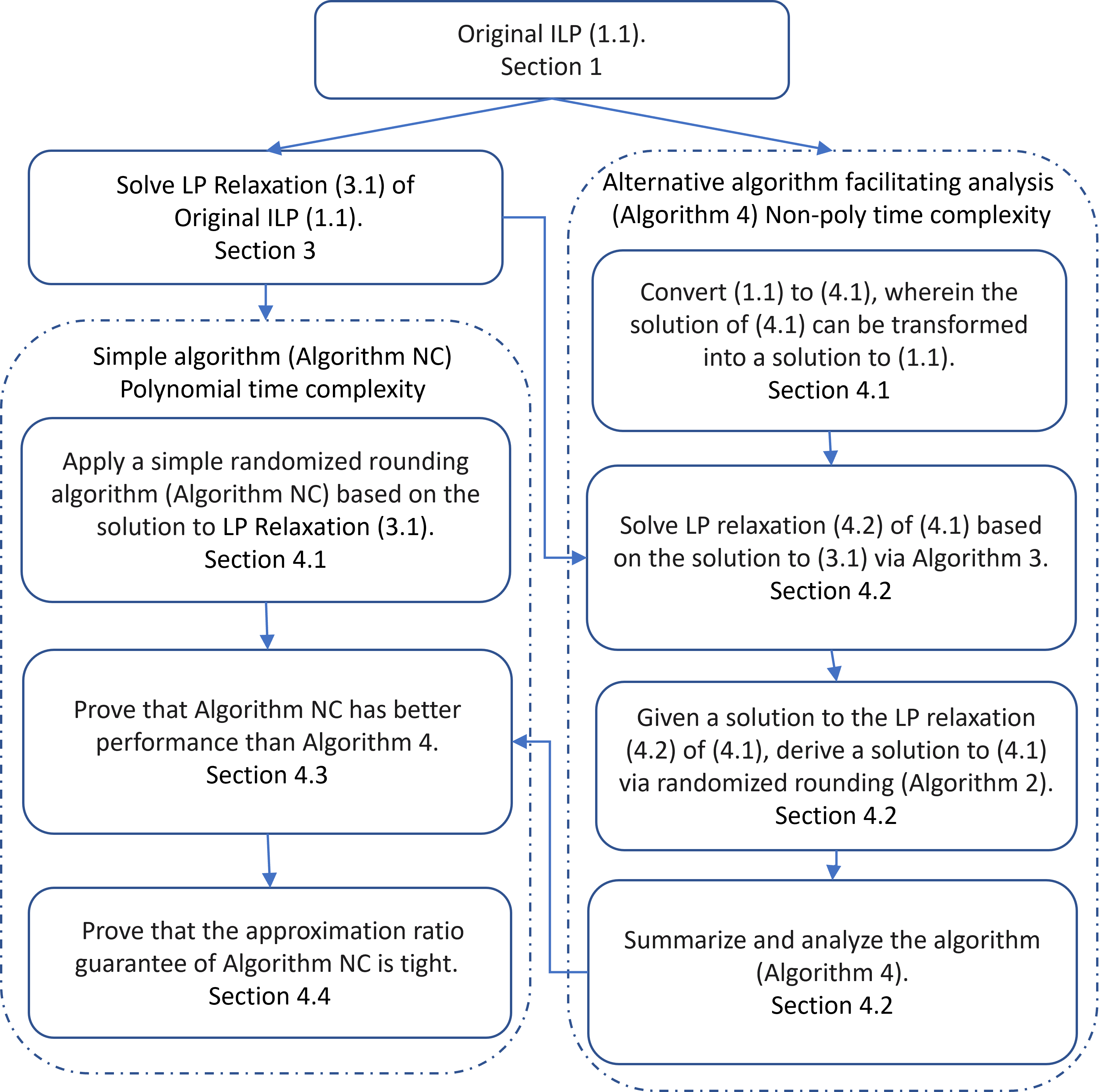
Figure 1: Approach to finding and analyzing a solution for (1.1).

4.1 A Simple Randomized Rounding Algorithm

Given an optimal solution to (3.1), we propose a simple randomized rounding algorithm for solving (1.1).

Algorithm NC.

Input: LP relaxation (3.1), and its optimal solution. Let $\widehat{n}_{b,l}$ be defined as in Remark 3.2. Let $\left\{\widehat{\lambda}_{b,l}^{(t)}:b\in[M],l\in\mathcal{L},t\in\left[\widehat{n}_{b,l}\right]\right\}$ represent the optimal solution to the LP relaxation (3.1).

Output: A (randomized) solution to (1.1).

Steps:

1. For each $b\in[M]$, a tuple $(l,t)$ is randomly selected (sampled) based on the selection probabilities given by $\widehat{\lambda}_{b,l}^{(t)}$. Denote the selected tuple for each $b\in[M]$ as $(b,l_{b},t_{b})$.

2. Given the sampling realization, for each OD pair $(i,j)\in D$, assume that $v_{1,l_{1},(i,j)}\geq v_{2,l_{2},(i,j)}\geq\ldots\geq v_{M,l_{M},(i,j)}$. Proceed by sequentially assigning $\theta_{b,l_{b},(i,j)}^{(t_{b})}$ to $b$ operating on line $l_{b}$, from $b=1$ to $b=M$. If the total assigned demand for the OD pair $(i,j)$ exceeds $d_{(i,j)}$, discard the excess part that was allocated last, ensuring that the total assigned demand does not exceed $d_{(i,j)}$. $\triangleleft$

The following observation is straightforward.

Lemma 4.1.

The demand assignments produced by Algorithm NC are integral.

Let $\Gamma$ be the optimal objective value of LP relaxation (3.1). We will prove the following theorem in Section 4.3 by demonstrating the superiority of Algorithm NC over auxiliary Algorithm 4 introduced in Section 4.2.

Theorem 4.2.

The expected reward of the solution obtained by Algorithm NC is at least

$$\left(1-\frac{1}{e}\right)\cdot\sum_{b\in[M]}\sum_{l\in\mathcal{L}_{b}}\sum_{t\in[n_{b,l}]}\sum_{(i,j)\in D}v_{b,l,(i,j)}{\theta}_{b,l,(i,j)}^{(t)}\widehat{\lambda}_{b,l}^{(t)}~{}=~{}\left(1-\frac{1}{e}\right)\Gamma.$$

4.2 An Alternative Algorithm Facilitating Analysis

In this section, we present an alternative randomized rounding algorithm to solve (1.1). The algorithm terminates in a finite, albeit non-polynomial, number of steps and focuses on solving an expanded-size ILP. We show that the alternative algorithm achieves the bound in Theorem 4.2, and that it is inferior to Algorithm NC, thereby proving Theorem 4.2.

4.2.1 Converting (1.1) to an Expanded-Size ILP

In Section 4.2.1, we study an altered ILP (4.1) where each OD pair’s demand is split into $d_{(i,j)}$ individuals. Let $P:=\sum_{(i,j)\in D}d_{(i,j)}$. Furthermore, let $\mathcal{P}_{ij}$ be a subset of $[P]$ such that $\left|\mathcal{P}_{ij}\right|=d_{(i,j)}$ and $\cup_{(i,j)\in D}\mathcal{P}_{ij}=[P]$. Note that the sets in the collection $\left\{\mathcal{P}_{ij}\right\}_{(i,j)\in D}$ are mutually exclusive. The elements of $\mathcal{P}_{ij}$ are identified with the individuals of the OD pair $(i,j)$. (Here, and in the rest of the paper, for brevity we use the expression “individual of the OD pair” to mean “individual from the OD pair’s demand”.) Define $\mathcal{I}_{b,l}$ as the set of all feasible assignment configurations of individuals to bus $b$ operating on line $l$. That is, every element in $\mathcal{I}_{b,l}$ represents a feasible allocation of individuals to bus $b$ on line $l$, respecting the bus capacity constraints. More formally, an element $S\in\mathcal{I}_{b,l}$ can be described by an element in the set below:

$$\widetilde{\mathcal{P}}(b,l):=\Bigg{\{} x_{(i,j),p}\in\{0,1\},~{}\forall(i,j)\in D,~{}p\in\mathcal{P}_{ij}:$$

$$\sum_{\begin{subarray}{c}(i,j):e\in r_{(i,j),l}\end{subarray}}\sum_{p\in\mathcal{P}_{ij}}x_{(i,j),p}\leq C_{b},~{}~{}\forall e\in r_{l}\Bigg{\}}~{}~{}~{}\mbox{ for }b\in[M],l\in\mathcal{L}_{b}.$$

Here, $r_{(i,j),l}$ is the subpath of line $l$ connecting the OD pair $(i,j)$, as defined in Section 1.

Given bus $b$, line $l$, an individual $p$ of OD pair $(i,j)$, and a feasible assignment configuration $S\in\mathcal{I}_{b,l}$, we say $p\in S$ if $p$ is assigned to bus $b$ operating on line $l$ in assignment configuration $S$.

Now the line planning problem can be formulated as follows:

$$\max_{X}~{}~{}~{} \sum_{(i,j)\in D}\sum_{p\in\mathcal{P}_{ij}}\sum_{b\in[M]}\sum_{l\in\mathcal{L}_{b}}\sum_{S\in\mathcal{I}_{b,l}:p\in S}v_{b,l,(i,j)}\cdot X_{b,l,S}$$ (4.1a)

$$s.t.~{}~{}~{} \sum_{l\in\mathcal{L}_{b}}\sum_{S\in\mathcal{I}_{b,l}}X_{b,l,S}=1~{}~{}~{}\forall b\in[M]$$ (4.1b)

$$\sum_{b\in[M]}\sum_{l\in\mathcal{L}_{b}}\sum_{S\in\mathcal{I}_{b,l}:p\in S}X_{b,l,S}\leq 1~{}~{}~{}\forall(i,j)\in D,~{}p\in\mathcal{P}_{ij}$$ (4.1c)

$$X_{b,l,S}\in\{0,1\}$$ (4.1d)

The first constraint ensures that each bus is assigned to a unique line $l$ and serves the individuals on that line according to a particular feasible assignment configuration $S\in\mathcal{I}_{b,l}$. The second constraint ensures that each individual of OD pair $(i,j)$ can be served by at most one bus.

Apparently, a feasible solution of (4.1) can be easily converted to a feasible solution for (1.1) with the same objective value, and vice versa. Hence, the optimal objective values of (4.1) and (1.1) are the same.

Consider the following linear relaxation of (4.1):

$$\max_{X}~{}~{}~{} \sum_{(i,j)\in D}\sum_{p\in\mathcal{P}_{ij}}\sum_{b\in[M]}\sum_{l\in\mathcal{L}_{b}}\sum_{S\in\mathcal{I}_{b,l}:p\in S}v_{b,l,(i,j)}\cdot X_{b,l,S}$$ (4.2a)

$$s.t.~{}~{}~{} \sum_{l\in\mathcal{L}_{b}}\sum_{S\in\mathcal{I}_{b,l}}X_{b,l,S}=1~{}~{}~{}\forall b\in[M]$$ (4.2b)

$$\sum_{b\in[M]}\sum_{l\in\mathcal{L}_{b}}\sum_{S\in\mathcal{I}_{b,l}:p\in S}X_{b,l,S}\leq 1~{}~{}~{}\forall(i,j)\in D,~{}p\in\mathcal{P}_{ij}$$ (4.2c)

$$X_{b,l,S}\in[0,1]$$ (4.2d)

Let $\Gamma^{\prime}$ be the optimal objective value of (4.2). A feasible solution to (4.2) can be easily converted into a feasible solution for (3.1) with the same objective value. Hence, $\Gamma\geq\Gamma^{\prime}$. We will show in Section 4.2.2 how to convert an optimal solution to (3.1) into a feasible solution for (4.2) with the same objective value, thus establishing $\Gamma\leq\Gamma^{\prime}$; this will imply that the optimal objective values of the LP relaxations (4.2) and (3.1) are the same ($\Gamma=\Gamma^{\prime}$).

For now we assume that we are given an optimal solution $\left\{\widehat{X}_{b,l,S}:~{}b\in[M],~{}l\in\mathcal{L}_{b},~{}S\in\mathcal{I}_{b,l}\right\}$ to (4.2), leaving the discussion of how to find it to Section 4.2.2. Using a modification of the randomized rounding approach from [7], now we derive an integer solution to (4.1).

Algorithm 2.

Input: LP relaxation (4.2), and its optimal solution: $\left\{\widehat{X}_{b,l,S}:~{}b\in[M],~{}l\in\mathcal{L}_{b},~{}S\in\mathcal{I}_{b,l}\right\}$.

Output: A (randomized) solution to (4.1).

Steps:

1. For each bus $b$, one candidate line $l$ with an assignment configuration $S$ is randomly selected (sampled) based on selection probabilities given by $\widehat{X}_{b,l,S}$.

2. If an individual $p$ of OD pair $(i,j)$ has been assigned to more than one bus, assign $p$ to the bus with the highest $R_{b,(i,j),p}$ value, where $R_{b,(i,j),p}$ is defined as:

   $$R_{b,(i,j),p}=\frac{\sum_{l\in\mathcal{L}_{b}}\sum_{S\in\mathcal{I}_{b,l}:p\in S}v_{b,l,(i,j)}\cdot\widehat{X}_{b,l,S}}{\sum_{l\in\mathcal{L}_{b}}\sum_{S\in\mathcal{I}_{b,l}:p\in S}\widehat{X}_{b,l,S}}.$$

$\triangleleft$

Theorem 4.3.

The expected objective value of the integer solution obtained using Algorithm 2 is at least

$$\left(1-\frac{1}{e}\right)\sum_{(i,j)\in D}\sum_{p\in\mathcal{P}_{ij}}\sum_{b\in[M]}\sum_{l\in\mathcal{L}_{b}}\sum_{S\in\mathcal{I}_{b,l}:p\in S}v_{b,l,(i,j)}\cdot\widehat{X}_{b,l,S}~{}=~{}\left(1-\frac{1}{e}\right)\Gamma^{\prime}.$$

To prove Theorem 4.3, it suffices to individually analyze the expected reward generated by the assignment of each individual of each OD pair. By showing the desired result for each individual assignment, we can conclude that the expected total reward meets the required bound. To do this, we need only to prove the lemma below.

Lemma 4.4.

By applying Algorithm 2, the expected reward generated from assigning individual $p$ of OD pair $(i,j)$ is at least

$$\left(1-\frac{1}{e}\right)\sum_{b\in[M]}\sum_{l\in\mathcal{L}_{b}}\sum_{S\in\mathcal{I}_{b,l}:p\in S}v_{b,l,(i,j)}\cdot\widehat{X}_{b,l,S}$$

.

Proof.

For the sake of analysis, we can assume without loss of generality that $R_{1,(i,j),p}\geq R_{2,(i,j),p}\geq\ldots R_{M,(i,j),p}$. Let us define a random variable $Z_{b}$ with the following probability distribution:

$$P\left(Z_{b}=v_{b,l,(i,j)}\right)=\sum_{S\in\mathcal{I}_{b,l}:p\in S}\widehat{X}_{b,l,S}$$

$$P(Z_{b}=0)=1-\sum_{l\in\mathcal{L}_{b}}\sum_{S\in\mathcal{I}_{b,l}:p\in S}\widehat{X}_{b,l,S}.$$

Additionally, define another set of indicator random variables $Z^{\prime}_{b}$ as follows: $Z^{\prime}_{1}$ is equal to 1 if $Z_{1}>0$. For $b>1$, $Z^{\prime}_{b}$ is equal to 1 only if $\sum_{j=1}^{b-1}Z^{\prime}_{j}=0$ and $Z_{b}>0$, else $Z^{\prime}_{b}=0$.

Consequently, $\mathbb{E}\left[\sum_{b\in[M]}Z^{\prime}_{b}\cdot Z_{b}\right]$ represents the expected reward derived from the assignment of individual $p$ of the OD pair $(i,j)$ according to Algorithm 2. Let $\lambda_{b}:=\sum_{l\in\mathcal{L}_{b}}\sum_{S\in\mathcal{I}_{b,l}:p\in S}\widehat{X}_{b,l,S}$. Then we have $\sum_{b\in[M]}\lambda_{b}=\sum_{b\in[M]}\sum_{l\in\mathcal{L}_{b}}\sum_{S\in\mathcal{I}_{b,l}:p\in S}\widehat{X}_{b,l,S}\leq 1$ and

$$\mathbb{E}\left[\sum_{b\in[M]}Z^{\prime}_{b}\cdot Z_{b}\right] =\sum_{b\in[M]}\mathbb{E}\left[Z_{b}|Z^{\prime}_{b}=1\right]\cdot P\left(Z^{\prime}_{b}=1\right)$$

$$=\sum_{b\in[M]}\mathbb{E}\left[Z_{b}|Z^{\prime}_{b}=1\right]\cdot\prod_{j=1}^{b-1}\left(1-\lambda_{j}\right)\lambda_{b}$$

$$= \sum_{b\in[M]}R_{b,(i,j),p}\prod_{j=1}^{b-1}\left(1-\lambda_{j}\right)\lambda_{b}\geq\left(1-\frac{1}{e}\right)\sum_{b\in[M]}R_{b,(i,j),p}\lambda_{b}$$ (4.3)

$$= \left(1-\frac{1}{e}\right)\sum_{b\in[M]}\sum_{l\in\mathcal{L}_{b}}\sum_{S\in\mathcal{I}_{b,l}:p\in S}v_{b,l,(i,j)}\cdot\widehat{X}_{b,l,S}$$

The inequality in (4.3) is due to [7, Lemma 2.1]. ∎

Remark 4.5.

The assignment problem considered in [7] is structurally different from that in (4.1). In the former, the reward generated from assigning an item (corresponding to an individual in (4.1)) to a container (corresponding to a bus in (4.1)) remains the same for all configurations feasible for this container that include the item. On the other hand, in the context (4.1), the reward is configuration-dependent since it depends also on the line.

Remark 4.6.

Another important point is that the conflict resolution approach of Algorithm 2 based on using values $R_{b,(i,j),p}$ is not the best for (4.1); clearly, resolving assignment conflicts based on sample-dependent values $v_{b,l_{b},(i,j)}$, where $l_{b}$ is the line selected (randomly) for bus $b$ in Algorithm 2, would result in a higher expected reward. The approach of Algorithm 2 is chosen specifically to meet the bound in Theorem 4.3 but at the same time to ensure that Algorithm NC has better performance, as will be shown later. Using values $R_{b,(i,j),p}$ is a new feature that can be used for analyzing performance of randomized algorithms for assignment problems with configuration-dependent rewards.

4.2.2 Generating an optimal solution for (4.2).

Our next goal is to show that an optimal solution to (3.1) can be converted to a feasible solution of (4.2) with the same objective value. The previous discussion implies that this will prove $\Gamma=\Gamma^{\prime}$ and that the converted solution is optimal for (4.2). Also, the construction will allow us to show that Algorithm NC has better performance than Algorithm 2, which will complete the proof of Theorem 4.2.

The idea of the approach. Let $\{\widehat{\lambda}_{b,l}^{(t)}\}$ be the obtained optimal solution to the LP relaxation (3.1). A natural idea is to represent each allocation variant $\theta_{b,l}^{(t)}$ that corresponds to a non-zero variable $\widehat{\lambda}_{b,l}^{(t)}$ with some assignment configurations $S\in\mathcal{I}_{b,l}$, splitting the value $\widehat{\lambda}_{b,l}^{(t)}$ between the corresponding variables $X_{b,l,S}$ of (4.2). The difficulty is that allocation variants $\theta_{b,l}^{(t)}$ are in “aggregate” form, specifying only the amounts of the demand of each OD pair allocated to bus - line combinations, while assignment configurations $S$ are in much more detailed form, actually listing specific individuals allocated; additionally, different allocation variants $\theta_{b,l}^{(t)}$ have different “weights” $\widehat{\lambda}_{b,l}^{(t)}$. This makes it non-obvious how to represent allocation variants with assignment configurations and how to split the corresponding “weights” $\widehat{\lambda}_{b,l}^{(t)}$ so as to ensure that the constraint (4.2c) is honored for each individual $p$. Since constraints (4.2c) are for each individual, selection of specific individuals for assignment configurations $S$, and the way of splitting $\widehat{\lambda}_{b,l}^{(t)}$ between the corresponding $X_{b,l,S}$, are important.

Note that we do not need to use (4.1) and (4.2) for solving LPRC; these formulations are introduced only for the sake of theoretical analysis, to prove Theorem 4.2. Hence, we do not need to worry about the computational complexity of the procedures related with the analysis of these formulations. Therefore, although the obtained optimal solution $\{\widehat{\lambda}_{b,l}^{(t)}\}$ to LP relaxation (3.1) is of polynomial size if we consider only non-zero variables, the corresponding “equivalent” solution to (4.2) that we are going to construct can be very large and the “procedure” of constructing it can be very long. With that in mind, we do the following. Each allocation variant $\theta_{b,l}^{(t)}$ that corresponds to a non-zero variable $\widehat{\lambda}_{b,l}^{(t)}$ will be represented by a large number of assignment configurations $S\in\mathcal{I}_{b,l}$ (some of which may be identical) each having aggregate demand allocation numbers the same as $\theta_{b,l}^{(t)}$ and a small “atom” weight $X_{b,l,S}$. The atom weights of all such assignment configurations will be the same irrespective of the allocation variant $\theta_{b,l}^{(t)}$ and the corresponding $\widehat{\lambda}_{b,l}^{(t)}$ that they represent, but the number of assignment configurations representing $\theta_{b,l}^{(t)}$ will be proportional to $\widehat{\lambda}_{b,l}^{(t)}$, so that the total of atom weights of all assignment configurations representing $\theta_{b,l}^{(t)}$ is $\widehat{\lambda}_{b,l}^{(t)}$. We will populate these assignment configurations with specific individuals in a greedy fashion, ensuring that all individuals from an OD pair’s demand are used in the same number of configurations. Since all configurations have the same atom weight and all individuals from an OD pair’s demand are used in the same number of configurations, and there are $d_{(i,j)}$ individuals for each OD pair $(i,j)$, and since values $\widehat{\lambda}_{b,l}^{(t)}$ satisfy constraints (3.1b) and (3.1d), the constraints of (4.2) will be met, and the objective value of this solution will be $\Gamma$.

Now we provide a more detailed overview.

Algorithm Overview: Let $\Delta$ be a small positive number such that $\frac{1}{\Delta}\in{\mathbb{Z}}$ and $\frac{\widehat{\lambda}_{b,l}^{(t)}}{\Delta}\in{\mathbb{Z}}$ for all $(b,l,t)$. Let $N_{b,l}^{(t)}:=\frac{\widehat{\lambda}_{b,l}^{(t)}}{\Delta}$. (Note that $N_{b,l}^{(t)}=0$ if $\widehat{\lambda}_{b,l}^{(t)}=0$.) For each tuple $(b,l,t,s)$ where $s\in\left[N_{b,l}^{(t)}\right]$, the algorithm creates a feasible assignment configuration, denoted by $S(b,l,t,s)$, that includes $\theta_{b,l,(i,j)}^{(t)}$ individuals from each OD pair $(i,j)$. Hence, there will be $N_{b,l}^{(t)}$ assignment configurations representing an allocation variant $\theta_{b,l}^{(t)}$, all having the same “aggregate” assignment numbers $\theta_{b,l,(i,j)}^{(t)}$ but possibly including different individuals. A greedy strategy guides the process of assigning specific individuals to these assignment configurations. In this process, for each individual we use a counter to track the number of assignment configurations that this individual has been assigned to; we use these counters to ensure that all individuals of an OD pair are used equally. Initially, individual counters are set to zero and all sets $S(b,l,t,s)$ are empty. The algorithm then iterates over OD pairs, populating $S(b,l,t,s)$ by selecting individuals with lower counter values from the corresponding OD pair and updating the counters respectively. The decision variables $X_{b,l,S(b,l,t,s)}$, which for simplicity will be denoted $X_{b,l,S(t,s)}$, that correspond to the created assignment configurations $S(b,l,t,s)$ in the LP relaxation (4.2) are all set to $\Delta$ (atom weight), while all other variables are set to zero.

Let $\widehat{n}_{b,l}$ be defined as in Remark 3.2. Below is the formal description of the algorithm.

Algorithm 3.

Input: $\left\{\widehat{\lambda}_{b,l}^{(t)},\Delta,N_{b,l}^{(t)}=\frac{\widehat{\lambda}_{b,l}^{(t)}}{\Delta}:b\in[M],l\in\mathcal{L}_{b},t\in\left[\widehat{n}_{b,l}\right]\right\}$ and $\left\{{\theta}_{b,l}^{(t)}:b\in[M],l\in\mathcal{L}_{b},t\in\left[\widehat{n}_{b,l}\right]\right\}$.

Output: $\left\{S(b,l,t,s)\text{ and }\widehat{X}_{b,l,S(t,s)}:b\in[M],l\in\mathcal{L}_{b},t\in\left[\widehat{n}_{b,l}\right],s\in\left[N_{b,l}^{(t)}\right]\right\}$

1. For each tuple $(b,l,t,s)$, initialize $S(b,l,t,s)=\emptyset$. For each $p\in[P]$, initialize a counter of $p$, denoted by $\#(p)$, as $0$.

2. Iterate over each OD pair $(i,j)\in D$, and do the following:

   1. Iterate over each tuple $(b,l,t,s)$, and do the following:

      1. Update $S(b,l,t,s)$ by including $\theta_{b,l,(i,j)}^{(t)}$ individuals from OD pair $(i,j)$ with the smallest $\theta_{b,l,(i,j)}^{(t)}$ counter values. Note that $\theta_{b,l,(i,j)}^{(t)}\leq d_{(i,j)}$.

      2. For the individuals of OD pair $(i,j)$ included in $S(b,l,t,s)$ in the previous step, increase their counter values by $1$.

3. $\widehat{X}_{b,l,S(t,s)}=\Delta$ for all $(b,l,t,s)$. All the other decision variables of $(\ref{LP-relaxation-detour})$ are set to be $0$. $\triangleleft$

Lemma 4.7.

For each $(b,l,t,s)$, the set $S(b,l,t,s)$ constructed by Algorithm 3 is a feasible assignment configuration for bus $b$ operating on line $l$. Specifically, it satisfies the following conditions:

1. Each individual is included at most once in $S(b,l,t,s)$.

2. It respects the capacity constraints for bus $b$ operating on line $l$.

Moreover, the solution for (4.2) obtained by Algorithm 3 satisfies constraints (4.2b) and (4.2c), and has objective value equal to $\Gamma$.

Proof.

Condition (i) is guaranteed by Step 2 of Algorithm 3. Condition (ii) is guaranteed since $S(b,l,t,s)$ include $\theta_{b,l,(i,j)}^{(t)}$ individuals of OD pair $(i,j)$, and $\theta_{b,l}^{(t)}$ is a point of $\mathcal{P}(b,l)$.

For each $b\in[M]$,

$$\sum_{l\in\mathcal{L}_{b}}\sum_{t\in\left[\widehat{n}_{b,l}\right]}\sum_{s\in\left[N_{b,l}^{(t)}\right]}\widehat{X}_{b,l,S(t,s)}=\sum_{l\in\mathcal{L}_{b}}\sum_{t\in\left[\widehat{n}_{b,l}\right]}\sum_{s\in\left[N_{b,l}^{(t)}\right]}\Delta=\sum_{l\in\mathcal{L}_{b}}\sum_{t\in\left[\widehat{n}_{b,l}\right]}\widehat{\lambda}_{b,l}^{(t)}=1.$$

Thus, Constraint (4.2b) is satisfied.

For each $p\in\mathcal{P}_{ij}$, we have that $\#(p)\leq\frac{1}{\Delta}$ after Algorithm 3 finishes. This is again ensured by Step 2 of Algorithm 3, and the facts that $\lvert\mathcal{P}_{ij}\rvert=d_{(i,j)}$ and

$$\sum_{b\in[M]}\sum_{l\in\mathcal{L}_{b}}\sum_{t\in\left[\widehat{n}_{b,l}\right]}\theta_{b,l,(i,j)}^{(t)}\cdot\widehat{\lambda}_{b,l}^{(t)}\leq d_{(i,j)}$$

$$\Rightarrow \sum_{b\in[M]}\sum_{l\in\mathcal{L}_{b}}\sum_{t\in\left[\widehat{n}_{b,l}\right]}\sum_{s\in\left[N_{b,l}^{(t)}\right]}\theta_{b,l,(i,j)}^{(t)}\cdot\Delta\leq d_{(i,j)}$$

$$\Rightarrow \sum_{b\in[M]}\sum_{l\in\mathcal{L}_{b}}\sum_{t\in\left[\widehat{n}_{b,l}\right]}\sum_{s\in\left[N_{b,l}^{(t)}\right]}\theta_{b,l,(i,j)}^{(t)}\leq d_{(i,j)}\cdot\frac{1}{\Delta}$$

Consequently, we have

$$\sum_{b\in[M]}\sum_{l\in\mathcal{L}_{b}}\sum_{(t,s):p\in S(b,l,t,s)}\widehat{X}_{b,l,S(t,s)}$$

$$= \sum_{b\in[M]}\sum_{l\in\mathcal{L}_{b}}\sum_{(t,s):p\in S(b,l,t,s)}\Delta$$

$$\leq \Delta\cdot\frac{1}{\Delta}\leq 1.$$

Therefore, Constraint (4.2c) is satisfied.

The objective value of the constructed solution is

$$\sum_{b\in[M]}\sum_{(i,j)\in D}\sum_{l\in\mathcal{L}_{b}}\sum_{t\in\left[\widehat{n}_{b,l}\right]}\sum_{s\in\left[N_{b,l}^{(t)}\right]}v_{b,l,(i,j)}\widehat{X}_{b,l,S(t,s)}\cdot\lvert S(b,l,t,s)\cap\mathcal{P}_{ij}\rvert$$

$$= \sum_{b\in[M]}\sum_{l\in\mathcal{L}_{b}}\sum_{t\in[\widehat{n}_{b,l}]}\sum_{s\in\left[N_{b,l}^{(t)}\right]}\sum_{(i,j)\in D}v_{b,l,(i,j)}{\theta}_{b,l,(i,j)}^{(t)}\widehat{\lambda}_{b,l}^{(t,s)}$$

$$= \sum_{b\in[M]}\sum_{l\in\mathcal{L}_{b}}\sum_{t\in[\widehat{n}_{b,l}]}\sum_{(i,j)\in D}v_{b,l,(i,j)}{\theta}_{b,l,(i,j)}^{(t)}\widehat{\lambda}_{b,l}^{(t)}=\Gamma.$$

This finishes the proof. ∎

Remark 4.8.

As follows from the previous discussion, Lemma 4.7 implies that $\Gamma=\Gamma^{\prime}$.

4.2.3 Summary of the Algorithm

Here we summarize the alternative (non-polynomial) algorithm defined in Section 4.2.1 and Section 4.2.2 for solving (1.1).

Algorithm 4.

Input: An instance of our line planning problem.

Output: A (randomized) solution to the given instance.

Steps:

1. Solve the LP relaxation (3.1) of (1.1). Let $\{\widehat{\lambda}_{b,l}^{(t)}\}$ represent the optimal solution to the LP relaxation (3.1). Let $\widehat{n}_{b,l}$ be defined as in Remark 3.2.

2. Define $\Delta$ as a small positive number such that $\frac{1}{\Delta}\in\mathbb{Z}$ and $\frac{\widehat{\lambda}_{b,l}^{(t)}}{\Delta}\in\mathbb{Z}$ for all $(b,l,t)$. Let $N_{b,l}^{(t)}:=\frac{\widehat{\lambda}_{b,l}^{(t)}}{\Delta}$.

3. Utilizing the optimal solution to (3.1), apply Algorithm 3 to solve the LP relaxation (4.2) of (4.1), providing a solution represented by $\widehat{X}_{b,l,S(t,s)}$ for $b\in[M]$, $l\in\mathcal{L}_{b}$, $t\in\left[\widehat{n}_{b,l}\right]$ and $s\in\left[N_{b,l}^{(t)}\right]$.

4. Apply Algorithm 2 to convert this LP solution into an integer solution to (4.1), thereby providing a solution to (1.1). $\triangleleft$

The theoretical guarantee for Algorithm 4 can be immediately derived from Lemma 4.7, Theorem 4.3, and Remark 4.8:

Theorem 4.9.

The expected reward obtained by applying Algorithm 4 is at least $\left(1-\frac{1}{e}\right)\Gamma$.

4.3 Algorithm NC Has Better Performance in Expectation

To prove Theorem 4.2, it suffices to prove the following theorem.

Theorem 4.10.

The expected reward generated by Algorithm NC is at least as large as that generated by Algorithm 4.

Proof.

Informally, the reason why Algorithm NC achieves a better expected reward than Algorithm 4 (or Algorithm 2) is as follows. Both Algorithm NC and Algorithm 2 start from an optimal solution to LP relaxation (3.1) (or its equivalent (4.2)), so at the randomization step (Step 1 of Algorithm NC or Step 1 of Algorithm 2) they generate the same expected reward (but the obtained solutions may be infeasible). However, at the next step (enforcing feasibility), they employ different strategies for resolving conflicts. Algorithm NC uses sample-dependent values $v_{k,l_{k},(i,j)}$ to decide which excessive allocated demand of each OD pair $(i,j)$ should be removed; so, this excess removal strategy is the best possible. Algorithm 2 uses sample-independent values $R_{b,(i,j),p}$ which is suboptimal (see Remark 4.6). Additionally, Algorithm 2 considers conflicts on “per individual” basis which can produce more conflicts to resolve, as opposed to conflicts in aggregate numbers (excess) in Algorithm NC.

Now we provide a more formal argument. Algorithm 4 starts by solving the LP relaxation (3.1). With its optimal solution at hand, it then employs Algorithm 3 to derive an optimal solution for (4.2). Then, a tuple $(l,S)$ is randomly sampled for each $b\in[M]$ by Algorithm 2. Denote the result of this sampling process as $(b,l_{b},S_{b})$ for every $b\in[M]$. Assume that the tuple $(b,l_{b},S_{b})$ corresponds to $(b,l_{b},t_{b},s_{b})$, meaning that $S_{b}=S(b,l_{b},t_{b},s_{b})$. Note that the probability of sampling the tuple $(l_{b},S_{b})$ for $b\in[M]$ by Algorithm 2 is the same as the probability of sampling $(l_{b},t_{b})$ for $b$ by Algorithm NC.

Given the sampling outcome, for every OD pair $(i,j)$, Algorithm 2 allocates a portion of its demand to each $(b,l_{b})$. This allocated demand does not exceed $\theta_{b,l_{b},(i,j)}^{(t_{b})}$, and the total assigned demand for each OD pair $(i,j)$ remains under $d_{(i,j)}$. It is clear that, given the sampling outcome, the reward gained in this process for OD pair $(i,j)$ cannot exceed the reward that would be obtained by the alternative procedure below (called “Eqv-Step”):

1. Suppose, for argument’s sake, that $v_{1,l_{1},(i,j)}\geq v_{2,l_{2},(i,j)}\geq\ldots\geq v_{M,l_{M},(i,j)}$. Assign consecutively demand $\theta_{b,l_{b},(i,j)}^{(t_{b})}$ of OD pair $(i,j)$ to $b$ on $l_{b}$, starting from $b=1$ and proceeding up to $b=M$. If the cumulative assigned demand for the OD pair $(i,j)$ exceeds $d_{(i,j)}$, we discard the surplus part that was assigned later, ensuring that the total assigned demand is $d_{(i,j)}$.

Observe that

1. Based on the definition of $\widehat{X}_{b,l,S(t,s)}$, the probability of the event that the sampling outcome in Algorithm 2 is $\left\{b,l_{b},t_{b},s\right\}$ for any $s\in[N_{b,l}^{(t)}]$ equals to the probability of obtaining $\left\{b,l_{b},t_{b}\right\}$ as the sampling outcome in Algorithm NC.

2. Eqv-Step is independent of the index $s$ and equivalent to Step 2 of Algorithm NC.

Thus the expected reward of the solution from Algorithm NC exceeds that from Algorithm 4.

∎

4.4 Tightness Result

In this section, we demonstrate that the approximation ratio for LPRC cannot exceed $\left(1-\frac{1}{e}\right)$, and thus that Algorithm NC achieves the optimal theoretical bound. We use a known hardness result for the max $k$-cover problem. We show that any instance of the max $k$-cover problem can be transformed into an instance of LPRC, which implies that the hardness result extends to LPRC.

Definition 4.11.

Given a set of $n$ elements: $G=\{p_{1},\dots,p_{n}\}$, and a collection of subsets of $G$: $F=\{G_{1},G_{2},\dots,G_{L}\}$, and an integer $k>0$, max $k$-cover is the problem of selecting $k$ sets from $F$ such that their union contains as many elements as possible.

The following hardness result has been proven in [5].

Theorem 4.12.

[5] For any constant $\epsilon>0$, unless $P=NP$, max $k$-cover problem cannot be approximated in polynomial time with an approximation ratio of $(1-\frac{1}{e}+\epsilon)$.

Theorem 4.13.

LPRC cannot be approximated in polynomial time within an approximation ratio of $(1-\frac{1}{e}+\epsilon)$ for any constant $\epsilon>0$, unless $P=NP$.

Proof.

Given an instance $(G=\{p_{1},\dots,p_{n}\},~{}F=\{G_{1},G_{2},\dots,G_{L}\},~{}k)$ of the max $k$-cover problem, we construct an equivalent instance of LPRC as follows. This instance will have $k$ buses, each with unit capacity, and a set of $L$ candidate lines.

The underlying network will have $2n$ vertices $o_{i,1},o_{i,2}$ for ${i\in[n]}$, and a set $D$ of $n$ OD pairs $(o_{i,1},o_{i,2})$ each having unit demand. The OD pair $(o_{i,1},o_{i,2})$ corresponds to the element $p_{i}$ and will be identified with this element. For any set $G_{j}:=\{p_{j_{1}},\dots,p_{j_{|G_{j}|}}\}$ from $F$ with $j_{1}\leq j_{2}\leq\dots\leq j_{|G_{j}|}$, we create a candidate line $j$ that can only serve the OD pairs from $G_{j}$, see the illustrative example in Figure 2. The line includes arcs from $o_{j_{i},1}$ to $o_{j_{i},2}$ for each $i\in\left[|G_{j}|\right]$, and arcs from $o_{j_{i},2}$ and $o_{j_{i+1},1}$ for each $i\in\left[|G_{j}|-1\right]$, thereby establishing a directed path. Note that line $j$ can only serve the OD pairs from $G_{j}$ since for any OD pair $p_{i^{\prime}}$ not in $G_{j}$, no path exists from $o_{i^{\prime},1}$ to $o_{i^{\prime},2}$ on line $j$. We assign a reward of $1$ for each unit of demand served by any bus on any line.

The equivalence of the obtained instance of LPRC and the original instance of max $k$-cover is straightforward. ∎

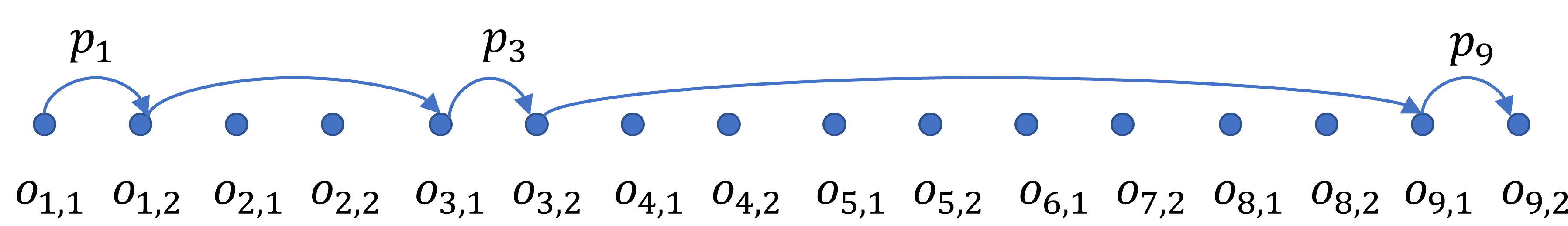
Figure 2: This figure illustrates a graph with $18$ vertices denoted by $\left\{o_{i,1},o_{i,2}\right\}_{i\in[9]}$. There are $9$ OD pairs represented as $\left\{p_{1},p_{2},\ldots,p_{9}\right\}$, where each pair $p_{i}$ plans to traverse from $o_{i,1}$ to $o_{i,2}$. Given a set $G_{1}:=\left\{p_{1},p_{3},p_{9}\right\}$, we construct line $1$ by sequentially connecting vertices $o_{1,1}$, $o_{1,2}$, $o_{3,1}$, $o_{3,2}$, $o_{9,1}$, and $o_{9,2}$. Note that this line can only serve OD pairs $p_{1}$, $p_{3}$, and $p_{9}$.

5 LPRC with Small Line Costs

In this section, we introduce a randomized algorithm tailored for LPRC instances where line costs are small. We formalize this condition with the following assumption given a constant $\eta\in(0,\frac{1}{2})$.

Assumption 5.1.

We assume that

$$\max_{b\in[M],l\in\mathcal{L}_{b},k\in[K]}c_{b,l}^{(k)}\leq\frac{\eta^{3}}{256K^{3}}.$$

Intuitive Overview: We use a randomized rounding mechanism similar to Algorithm NC but with somewhat smaller selection probabilities, introducing some additional probability that some buses will not be utilized. With that, for each resource, the expected resource usage will be somewhat smaller than the limit; then, since costs are small, the probability of exceeding the resource limit will be small. If the randomized solution exceeds the limit for some resource, we discard the solution (do not utilize the buses at all); since the probability of exceeding the resource limit is small, this does not affect significantly the expected reward.

Algorithm LC.

Input: LP relaxation (3.1), and its optimal solution $\left\{\widehat{\lambda}_{b,l}^{(t)}:b\in[M],l\in\mathcal{L}_{b},t\in\left[\widehat{n}_{b,l}\right]\right\}$, where $\widehat{n}_{b,l}$ is defined as in Remark 3.2.

Output: A (randomized) solution to (1.1).

Steps:

1. Let $q=\frac{4}{\eta}$ and $\epsilon=\frac{1}{q\cdot K}$. Observe that $\epsilon<\frac{\eta}{2}$. For each $b\in[M]$, sample a tuple $(l,t)$ with the selection probability given by $(1-\epsilon)\widehat{\lambda}_{b,l}^{(t)}$. Denote the sampled tuple for each $b\in[M]$ as $(b,l_{b},t_{b})$. The total of the selection probabilities for bus $b$ is less than 1, so if no tuple is selected, the bus is not used (assigned to a “dummy” line with zero costs and rewards).

2. Same as Step 2 in Algorithm NC.

3. If the solution meets the resource constraints, it becomes the final output. Otherwise, no lines are assigned to buses, and the reward generated is $0$. $\triangleleft$

Recall that $\Gamma:=\sum_{b\in[M]}\sum_{l\in\mathcal{L}_{b}}\sum_{t\in[n_{b,l}]}\sum_{(i,j)\in D}v_{b,l,(i,j)}{\theta}_{b,l,(i,j)}^{(t)}\widehat{\lambda}_{b,l}^{(t)}$ is the optimal objective value of the LP relaxation (3.1). We first analyze the solution provided by Steps 1 and 2 of Algorithm LC.

Lemma 5.2.

The randomized solution returned by Steps 1 and 2 of Algorithm LC has the following properties:

1. The expected return is at least $\left(1-\frac{1}{e}-\epsilon\right)\Gamma$.

2. Consider the event that the solution uses more than $\psi$ units of at least one resource, where $\psi\geq 1$. The probability of this event occurring is bounded above by $K\cdot e^{-(\psi\epsilon^{2})/(4\delta)}$, where $\delta=\frac{\eta^{3}}{256K^{3}}$.

3. If the solution uses no more than $\psi+1$ units of each resource, the resulting reward is bounded above by $(\psi+1)\cdot\Gamma$.

Proof.

Property (1) can be established by employing an analysis similar to that used in the proof of Theorem 4.2. The presence of the term $\epsilon$ in the approximation ratio arises from the adjustment of the sampling probabilities by a scaling factor of $(1-\epsilon)$.

Property (2) will be proven by applying Chernoff bounds [14]. Particularly, let $Y_{b,l}$ be the random indicator variable denoting the event that bus $b$ is assigned to line $l$. Note that if $Y_{b,l}=0$ for all $l\in\mathcal{L}_{b}$, then it means that bus $b$ is not utilized in the randomized solution. For a given $k\in[K]$, we have that

$$P\left(\sum_{b\in[M]}\sum_{l\in\mathcal{L}_{b}}Y_{b,l}\cdot c_{b,l}^{(k)}\geq\psi(1+\epsilon)(1-\epsilon)\right)=P\left(\sum_{b\in[M]}\sum_{l\in\mathcal{L}_{b}}Y_{b,l}\cdot\frac{c_{b,l}^{(k)}}{\delta}\geq\psi(1+\epsilon)\frac{(1-\epsilon)}{\delta}\right)\leq e^{-(\psi\epsilon^{2})/(4\delta)}$$

The last inequality is due to $\sum_{l\in\mathcal{L}_{b}}Y_{b,l}\cdot\frac{c_{b,l}^{(k)}}{\delta}\in[0,1]$ according to Assumption 5.1 , and $\sum_{b\in[M]}\sum_{l\in\mathcal{L}_{b}}\mathbb{E}\left[Y_{b,l}\right]\cdot c_{b,l}^{(k)}\leq(1-\epsilon)$, and Chernoff bounds. Now by taking a union bound over all $K$ resources, we can finish the proof.

Property (3) can be verified using concavity of the optimal objective value of a maximization linear programming problem with respect to right-hand sides of resource limit constraints. ∎

The following theorem establishes the expected approximation ratio of the randomized solution generated by Algorithm LC. The underlying intuition for the proof is that Steps 1 and 2 of Algorithm LC yield a solution with an expected approximation ratio of $\left(1-\frac{1}{e}-\epsilon\right)$. Violation of the resource constraints occurs with low probability, and the objective values are upper-bounded due to Lemma 5.2. Consequently, we demonstrate that the feasible solutions have an expected value closely approximating $\left(1-\frac{1}{e}-\epsilon\right)$.

Theorem 5.3.

The expected reward of the solution obtained by Algorithm LC is at least $\left(1-\frac{1}{e}-\eta\right)\cdot\Gamma$ under Assumption 5.1.

Proof.

Let $q=\frac{4}{\eta}$ and $\delta=\frac{1}{4q^{3}K^{3}}=\frac{\eta^{3}}{256K^{3}}$. Let $\mathcal{B}_{\psi}$ be the event that Steps 1 and 2 of Algorithm LC return a randomized solution which utilizes at least $\psi$ units for one or more resources, but does not exceed $\psi+1$ units for any resource. We define $P_{\psi}:=P(\mathcal{B}_{\psi})$ and

$$E_{\psi}:=\mathbb{E}\left[\text{Objective value of the randomized solution generated by Step \ref{alg-step:LC-sample} and \ref{alg-step:LC-rounding} of Algorithm \ref{alg:low-costs-feasible}}~{}\Big{|}~{}\mathcal{B}_{\psi}\right].$$

With this notation, $E_{0}\cdot P_{0}$ is the expected objective value of the solution yielded by Algorithm LC.

By definitions and Lemma 5.2, we have that

$$\left(1-\frac{1}{e}-\epsilon\right)\Gamma\leq E_{0}\cdot P_{0}+\sum_{\psi=1}^{\infty}E_{\psi}\cdot P_{\psi}$$

$$\leq E_{0}\cdot P_{0}+\sum_{\psi=1}^{\infty}(\psi+1)\Gamma\cdot K\cdot e^{-\psi\epsilon^{2}/4\delta}=E_{0}\cdot P_{0}+\Gamma\cdot\sum_{\psi=1}^{\infty}(\psi+1)\cdot K\cdot e^{-\psi Kq}$$

$$\leq E_{0}\cdot P_{0}+2\Gamma\cdot\sum_{\psi=1}^{\infty}\psi\cdot K\cdot e^{-\psi Kq}\leq E_{0}\cdot P_{0}+2\Gamma\cdot\sum_{t=1}^{\infty}t\cdot e^{-t\cdot q}$$

$$\leq E_{0}\cdot P_{0}+\frac{2}{q}\cdot\Gamma=E_{0}\cdot P_{0}+\frac{\eta}{2}\cdot\Gamma.$$

The last inequality is due to the fact that $q=\frac{4}{\eta}>4$, and

$$\sum_{t=1}^{\infty}t\cdot e^{-t\cdot q}=e^{-q}+\sum_{t=2}^{\infty}t\cdot e^{-t\cdot q}\leq e^{-q}+\int_{1}^{\infty}(x+1)e^{-x\cdot q}dx=\frac{e^{-q}}{q}\cdot(2+\frac{1}{q}+q)\leq\frac{1}{q}.$$

Since $\epsilon\leq\frac{\eta}{2}$, we have $E_{0}\cdot P_{0}\geq\left(1-\frac{1}{e}-\eta\right)\cdot\Gamma$. ∎

6 LPRC with General Line Costs

In this section, we introduce an approximation algorithm for general LPRC that achieves an expected approximation ratio of $\left(\frac{1}{2}-\frac{1}{2e}-\eta\right)$ for any constant $\eta\in(0,1/4)$. The algorithm categorizes the set of candidate lines into two distinct subsets: the first consists of low-cost candidate lines, and the second comprises the remaining candidate lines. We consider separately two subproblems: the problem restricted to the low-cost lines, and the problem restricted to the other lines. For the first subproblem, we employ Algorithm LC to find a solution. For the second subproblem, we resort to enumeration: we evaluate each enumerated scenario (a feasible assignment of buses to the lines) by solving the corresponding LP-relaxation, choose the scenario with the best LP-relaxation objective value, and apply Algorithm NC to this scenario. The algorithm ultimately selects the better of the two obtained solutions as the final output.

Remark 6.1.

The algorithm described below uses a slightly different logic: instead of obtaining randomized solutions for both the problem restricted to the low-cost lines and the problem restricted to the best (in terms of the LP relaxation objective value) enumerated scenario, we obtain a randomized solution for only one of these two problems (one that has a better LP relaxation objective value). Both versions have the same theoretical guarantee, with the same arguments.

Before detailing the algorithm, it is essential to define some specific sets and functions for formalization.

Definition 6.2.

Consider an instance (1.1) of LPRC. Let $\mathcal{A}$ be the set of all binary vectors $\omega=(\omega_{b,l})_{b\in[M],l\in\mathcal{L}_{b}}$ such that the following conditions are met: $\sum_{b\in[M],l\in\mathcal{L}_{b}}c_{b,l}^{(k)}\cdot\omega_{b,l}\leq 1$, for all $k\in[K]$, and $\sum_{l\in\mathcal{L}_{b}}\omega_{b,l}=1$, for all $b\in[M]$.

We introduce a function $f_{L}:\mathcal{A}\rightarrow\mathbb{Q}_{+}$. For $\omega\in\mathcal{A}$, $f_{L}(\omega)$ denotes the optimal objective value for the LP relaxation (3.1) subject to the additional constraints that $\lambda_{b,l}^{(t)}=0$ whenever $\omega_{b,l}=0$. We use $\text{LP}(\omega)$ to denote this restricted LP formulation.

Thus, each element in $\mathcal{A}$ specifies an assignment of candidate lines to buses that complies with the resource constraints, and $\mathcal{A}$ includes all such assignments. Additionally, $\text{LP}(\omega)$ is the LP relaxation of LPRC with the candidate line assignments fixed as defined by $\omega$.

Definition 6.3.

Given a constant $\delta\in(0,1)$, for each $b\in[M]$, define the set $\mathcal{L}_{b}^{\delta}$ as follows:

$$\mathcal{L}_{b}^{\delta}:=\left\{l\in\mathcal{L}_{b}:c_{b,l}^{(k)}\leq\delta\text{ for all }k\in[K]\right\}.$$

This set contains the candidate lines of bus $b$ for which all associated costs are not greater than $\delta$. Define the set $\mathcal{A}_{\delta}$ as:

$$\mathcal{A}_{\delta}:=\left\{\omega\in\mathcal{A}:\omega_{b,l}=0\text{ if }l\in\mathcal{L}_{b}^{\delta}\right\}.$$

This set includes all feasible line assignments limited to lines not in $\mathcal{L}_{b}^{\delta}$.

Let $\text{LP}_{\delta}$ be the LP relaxation (3.1) subject to extra constraints $\lambda_{b,l}^{(t)}=0$ whenever $l\notin\mathcal{L}_{b}^{\delta}$, and let $\Gamma_{\delta}$ be its optimal objective value. $\text{LP}_{\delta}$ represents the LP relaxation of LPRC including only the lines with all costs not greater than $\delta$.

Algorithm Overview: The core concept of the algorithm is to initially identify a candidate line assignment $\omega^{*}$ in $\mathcal{A}_{\delta}$ that yields the best LP-relaxation objective value $f_{L}(\omega^{*})$, and then compare $f_{L}(\omega^{*})$ with the objective value $\Gamma_{\delta}$ of $\text{LP}_{\delta}$. Subsequently, we apply the appropriate randomized rounding algorithm to the better (in terms of the optimal objective value) of these two LP relaxations, to obtain a final solution for LPRC. (Alternatively, we can apply the appropriate randomized rounding to the optimal solution of $\text{LP}_{\delta}$ and to the optimal solution of $\text{LP}(\omega^{*})$, and choose the best of the two obtained solutions.)

Algorithm C.

Input: An instance of LPRC (1.1), and $\eta\in\left(0,\frac{1}{2}\right)$.

Output: A (randomized) solution to (1.1).

Steps:

1. Define $q=\frac{4}{\eta}$ and $\delta=\frac{1}{4q^{3}K^{3}}=\frac{\eta^{3}}{256K^{3}}$. Solve $LP(\omega)$ for all $\omega\in\mathcal{A}_{\delta}$. Let $\omega^{*}\in\operatorname*{argmax}_{\omega\in\mathcal{A}_{\delta}}\left\{f_{L}(\mathbf{\omega})\right\}.$

2. If $\Gamma_{\delta}\geq f_{L}(\mathbf{\omega^{*}})$, then apply Algorithm LC to derive a solution to (1.1) based on $\text{LP}_{\delta}$.

3. Otherwise, apply Algorithm NC to derive a solution to (1.1) based on $\text{LP}(\omega^{*})$. $\triangleleft$

The following result guarantees that Algorithm C can be completed in polynomial time. Note that according to the assumptions made, $\frac{K}{\delta}$ is a constant.

Lemma 6.4.

Let $L:=\max_{b\in[M]}|\mathcal{L}_{b}|$. Then, we can bound $|\mathcal{A}_{\delta}|$ as follows:

$$|\mathcal{A}_{\delta}|\leq\frac{K}{\delta}\cdot(M\cdot L)^{\frac{K}{\delta}}.$$

Proof.

By the pigeonhole principle, at most $\frac{K}{\delta}$ lines with at least one type of cost larger than $\delta$ can be utilized while satisfying all resource constraints. Since each bus can choose from a maximum of $L$ candidate lines, the bound on $|\mathcal{A}_{\delta}|$ is established. ∎

The next lemma is needed for performance analysis.

Lemma 6.5.

$$\max\left\{f_{L}(\mathbf{\omega^{*}}),\Gamma_{\delta}\right\}\geq\frac{1}{2}\text{OPT}_{\text{IP}},$$

where $\text{OPT}_{\text{IP}}$ is the optimal objective value of LPTR.

Proof.

Define the set $\overline{\mathcal{A}}_{\delta}$:

$$\overline{\mathcal{A}}_{\delta}:=\left\{\omega\in\mathcal{A}:\omega_{b,l}=0\text{ if }l\notin\mathcal{L}_{b}^{\delta}\right\}.$$

Given the preceding definitions, for each $\omega\in\mathcal{A}$, vectors $\omega^{\prime}\in\mathcal{A}_{\delta}$ and $\omega^{\prime\prime}\in\overline{\mathcal{A}}_{\delta}$ exist such that $\omega^{\prime}+\omega^{\prime\prime}=\omega$. Consequently, the inequality $\Gamma_{\delta}+f_{L}(\omega^{\prime})\geq f_{L}(\omega)$ holds. This follows from the observation that a feasible solution for $\text{LP}(\omega)$ can be decomposed into distinct solutions for $\text{LP}_{\delta}$ and $\text{LP}(\omega^{\prime})$. Thus we have

$$\max\left\{f_{L}(\mathbf{\omega^{*}}),\Gamma_{\delta}\right\}\geq\frac{1}{2}\max_{\omega\in\mathcal{A}_{\delta}}\left(\Gamma_{\delta}+f_{L}(\omega)\right)\geq\frac{1}{2}\max_{\omega\in\mathcal{A}}f_{L}(\omega)\geq\frac{1}{2}\text{OPT}_{\text{IP}}.$$

∎

Combining Theorem 4.2, Theorem 5.3 and Lemma 6.5 immediately leads to the following result.

Theorem 6.6.

The expected approximation ratio of the solution given by Algorithm C is at least $\frac{1}{2}-\frac{1}{2e}-\eta$ for any constant $\eta\in(0,1/4)$.

7 LPRC with $\tau-$Tolerance in Resource Constraints

In this section, we present a randomized approximation algorithm with expected approximation ratio $\left(1-\frac{1}{e}-\eta\right)$ while ensuring that the solution utilizes no more than $1+\tau$ units of each resource type, for any given constants $\eta,\tau\in\left(0,\frac{1}{2}\right)$. It is worth noting that this approximation ratio is nearly tight. Specifically, when all costs are set to $0$, the hardness result from Theorem 4.13 can be directly applied here.

Algorithm Overview: In our algorithm, we enumerate all feasible line assignments restricted to the lines with at least one type of cost exceeding a predefined threshold; such lines will be called high-cost lines, and such feasible assignments will be called high-cost assignments. As shown in Section 6, the number of high-cost assignments is polynomial. For each enumerated case of a high-cost assignment, we adjust the remaining resources by removing those consumed by the assigned lines, and then augment each type of the residual resource by $\tau$. After scaling, the adjusted residual resources can then be used for the lines with all costs below the threshold (low-cost lines). Then, a modified version of the LP relaxation (3.1) is solved for each enumerated case where assignment of large-cost lines is fixed according to the case, and the case with the largest objective value of the modified LP relaxation is selected. Then, Algorithm LC is applied to the optimal solution of the modified LP relaxation for the selected case, and the obtained solution is presented as the final output.

Below, we define the modified LP relaxation. The notation introduced in the previous section applies.

Definition 7.1.

Given $\delta\leq\tau\in(0,\frac{1}{2})$, for each feasible vector $\omega\in\mathcal{A}_{\delta}$, let $\text{LP}_{\delta,\tau}(\omega)$ denote the modified LP relaxation (3.1). In $\text{LP}_{\delta,\tau}(\omega)$, the following adjustments are made:

1. Add constraints $\lambda_{b,l}^{(t)}=0$ whenever $l\notin\mathcal{L}_{b}^{\delta}$ and $\omega_{b,l}=0$.

2. Add constraints $\lambda_{b,l}^{(t)}=0$ whenever $\sum_{l^{\prime}\in\mathcal{L}_{b}}\omega_{b,l^{\prime}}=1$ and $\omega_{b,l}=0$.

3. Replace $c_{b,l}^{(k)}$ with $\widehat{c}_{b,l}^{(k)}$, where $\widehat{c}_{b,l}^{(k)}=0$ if $l\notin\mathcal{L}_{b}^{\delta}$, and $\widehat{c}_{b,l}^{(k)}=\frac{{c}_{b,l}^{(k)}}{1-\sum_{b,l}c_{b,l}^{(k)}\omega_{b,l}+\tau}$ otherwise.

4. Define $f_{L}^{{\delta,\tau}}:\mathcal{A}_{\delta}\rightarrow\mathbb{R}_{+}$. For each $\omega\in\mathcal{A}_{\delta}$, let $f_{L}^{\delta,\tau}(\mathbf{\omega})$ be the optimal objective value of $\text{LP}_{\delta,\tau}(\mathbf{\omega})$.

Step 1 filters out high-cost lines not in $\omega$. Step 2 ensures that buses assigned to the lines included in $\omega$ cannot be used for other lines. Step 3 sets the costs to $0$ for the high-cost lines (lines not in $\mathcal{L}_{b}^{\delta}$) and scales the costs for the low-cost lines to account for the resources consumed by the assigned high-cost lines and the adjustment of the resource limit by $\tau$ since the right-hand sides of all resource constraints in LP relaxation (3.1) are 1.

Since we apply scaling of the costs of low-cost lines, we need to make sure that after the scaling the conditions of applicability of Algorithm LC are still met. This is done by a proper choice of $\delta$.

Lemma 7.2.

Given $\tau,\eta\in(0,\frac{1}{2})$, let $q=\frac{4}{\eta}$ and $\delta=\frac{1}{4q^{3}K^{3}}\cdot\tau$. For any vector $\omega\in\mathcal{A}_{\delta}$ and its associated $\text{LP}_{\delta,\tau}(\mathbf{\omega})$, the parameter $\left(\widehat{c}_{b,l}^{(k)}\right)_{b\in[M],l\in\mathcal{L}_{b},k\in[K]}$ satisfies the criterion specified in Assumption 5.1. Specifically, we have:

$$\max_{b\in[M],l\in\mathcal{L}_{b},k\in[K]}\widehat{c}_{b,l}^{(k)}\leq\frac{\eta^{3}}{256K^{3}}.$$

Therefore, we can apply Algorithm LC to $\text{LP}_{\delta,\tau}(\mathbf{\omega})$ with costs set as $\left(\widehat{c}_{b,l}^{(k)}\right)_{b\in[M],l\in\mathcal{L}_{b},k\in[K]}$.

Proof.

The result is established through the following inequalities:

$$\widehat{c}_{b,l}^{(k)} \leq\frac{\delta}{1-\sum_{b,l}c_{b,l}^{(k)}\omega_{b,l}+\tau}\leq\frac{\delta}{\tau}\leq\frac{1}{4q^{3}K^{3}}=\frac{\eta^{3}}{256K^{3}}.$$

∎

We are now ready to outline our algorithm, guided by Lemma 7.2 in choosing the line cost threshold based on $\eta$ and $\tau$.

Algorithm C-Tol.

Input: An instance of LPRC (1.1), and $\tau,\eta\in\left(0,\frac{1}{2}\right)$.

Output: A (randomized) solution to (1.1).

Steps:

1. Define $q=\frac{4}{\eta}$ and $\delta=\frac{1}{4q^{3}K^{3}}\cdot\tau$.

2. For each $\omega\in\mathcal{A}_{\delta}$, compute $f_{L}^{{\delta,\tau}}(\omega)$. Let $\omega^{*}:=\operatorname*{argmax}_{\omega\in\mathcal{A}_{\delta}}f_{L}^{{\delta,\tau}}(\omega)$.

3. Apply Algorithm LC to $\text{LP}_{\delta,\tau}(\omega^{*})$ with costs set as $\left(\widehat{c}_{b,l}^{(k)}\right)_{b\in[M],l\in\mathcal{L}_{b},k\in[K]}$. To clarify, the final solution adheres to the following conditions: $\sum_{b\in[M],l\in\mathcal{L}_{b}}\widehat{c}_{b,l}^{(k)}\cdot\widetilde{\lambda}_{b,l}\leq 1.$ Here, $\left(\widetilde{\lambda}_{b,l}\right)_{b\in[M],l\in\mathcal{L}_{b}}$ is a binary vector that indicates whether bus $b$ operates on line $l$ in the final solution. $\triangleleft$

The following results provide theoretical performance guarantees for Algorithm C-Tol. The key insight is that Lemma 7.2 enables the application of Algorithm LC to the optimal solution of the modified LP relaxation for the enumerated case with the best optimal objective value of the corresponding modified LP relaxation, with the theoretical guarantee provided by Theorem 5.3, and that the optimal objective value of this modified LP relaxation is an upper bound for the optimal reward in LPRC.

Lemma 7.3.

Given an instance of LPRC (1.1) and $\tau,\eta\in(0,\frac{1}{2})$, let $\text{OPT}_{\text{IP}}$ be the optimal objective value for the instance. With the same notations as in Algorithm C-Tol, we have that $\max_{\omega\in\mathcal{A}_{\delta}}f_{L}^{{\delta,\tau}}(\omega)\geq\text{OPT}_{\text{IP}}.$

Proof.

For an optimal solution to (1.1), let $\widehat{\lambda}_{b,l}=1$ if bus $b$ operates on line $l$, and $0$ otherwise. Let $\widehat{\xi}_{b,l,(i,j)}$ be the number of passengers from OD pair $(i,j)$ assigned to bus $b$ on line $l$ in the solution. Let $\widetilde{\omega}_{b,l}=\widehat{\lambda}_{b,l}$ if $l\notin\mathcal{L}_{b}^{\delta}$, and $0$ otherwise. Then according to the definition of $\mathcal{A}_{\delta}$, we have that $\mathbf{\widetilde{\omega}}:=\left(\widetilde{\omega}_{b,l}\right)_{b\in[M],l\in\mathcal{L}_{b}}\in\mathcal{A}_{\delta}$. Without loss of generality, assume $\theta_{b,l,(i,j)}^{(1)}=\widehat{\xi}_{b,l,(i,j)}$, $\lambda_{b,l}^{(1)}=\widehat{\lambda}_{b,l}$ and $\lambda_{b,l}^{(t)}=0$ for all $t\geq 2$, $(i,j)\in D$, $b\in[M]$ and $l\in\mathcal{L}_{b}$. Then it can be checked that this defines a feasible solution to $\text{LP}_{\delta,\tau}\left(\mathbf{\widetilde{\omega}}\right)$, and its objective value is $\text{OPT}_{\text{IP}}$. Therefore, we have that $\text{OPT}_{\text{IP}}\leq f_{L}^{{\delta,\tau}}\left(\mathbf{\widetilde{\omega}}\right)\leq\max_{\omega\in\mathcal{A}_{\delta}}f_{L}^{{\delta,\tau}}(\omega)$. ∎

Theorem 7.4.

Algorithm C-Tol has an expected approximation ratio of at least $\left(1-\frac{1}{e}-\eta\right)$ while using at most $1+\tau$ units of each resource.

Proof.

Due to Lemma 7.2, we can directly apply Theorem 5.3 to demonstrate that the expected objective value of the solution returned by Algorithm C-Tol is at least $\left(1-\frac{1}{e}-\eta\right)f_{L}^{{\delta,\tau}}(\omega^{*})$. This, in conjunction with Lemma 7.3, establishes the approximation ratio.

Let $\left(\widetilde{\lambda}_{b,l}\right)_{b\in[M],l\in\mathcal{L}_{b}}$ be the binary vector that indicates whether bus $b$ operates on line $l$ in the solution returned by Algorithm C-Tol. By the definition of $\text{LP}_{\delta,\tau}(\mathbf{\omega^{*}})$ and Algorithm LC, we observe that $\widetilde{\lambda}_{b,l}=0$ whenever $l\notin\mathcal{L}_{b}^{\delta}$ and $\omega_{b,l}^{*}=0$, and $\widetilde{\lambda}_{b,l}\leq 1$ otherwise. This leads to

$$\sum_{b\in[M],l\in\mathcal{L}_{b}}c_{b,l}^{(k)}\cdot\widetilde{\lambda}_{b,l}\leq \sum_{b,l}c_{b,l}^{(k)}\omega^{*}_{b,l}+\sum_{b\in[M],l\in\mathcal{L}_{b}^{\delta}}c_{b,l}^{(k)}\cdot\widetilde{\lambda}_{b,l}$$

$$= \sum_{b,l}c_{b,l}^{(k)}\omega^{*}_{b,l}+\left(1-\sum_{b,l}c_{b,l}^{(k)}\omega^{*}_{b,l}+\tau\right)\cdot\sum_{b\in[M],l\in\mathcal{L}_{b}^{\delta}}\frac{c_{b,l}^{(k)}}{1-\sum_{b,l}c_{b,l}^{(k)}\omega^{*}_{b,l}+\tau}\cdot\widetilde{\lambda}_{b,l}$$

$$= \sum_{b,l}c_{b,l}^{(k)}\omega^{*}_{b,l}+\left(1-\sum_{b,l}c_{b,l}^{(k)}\omega^{*}_{b,l}+\tau\right)\cdot\sum_{b\in[M],l\in\mathcal{L}_{b}^{\delta}}\widehat{c}_{b,l}^{(k)}\cdot\widetilde{\lambda}_{b,l}\leq 1+\tau$$

Hence, the upper bound on the utilization of the $k$-th resource is $1+\tau$. ∎

8 Numerical experiments (Ongoing)

We conduct numerical experiments for Algorithm NC based on the data provided in Bertsimas et al. [2]. The experiments are conducted using the road network of the greater Boston area. Trip requests data is obtained from the Massachusetts Bay Transit Authority [13]. The total demand consists of $93,826$ passenger requests, with $597$ origin-destination pairs. For more detailed information about the data, please refer to [2].

We conduct numerical simulations for four sets of buses: $600$, $800$, $1000$, and $1200$ buses, respectively. Each experiment includes bus capacities of $25$, $30$, $35$, and $40$ passengers, with each capacity represented by a quarter of all buses (so, for example, if the total number of buses is 600, 150 of them have capacity 25). A candidate set of $1000$ lines is generated by following the method introduced by Silman et al. [17]. All the buses share the same candidate line set in the experiments.

When a passenger takes line $l$ on bus $b$ with capacity $C_{b}$, we calculate the reward based on their subroute distance $D_{l}$ on line $l$ and the shortest distance between their origin and destination, $D_{s}$. The reward is set to be $\max\left\{0,\frac{1.5\cdot D_{s}-D_{l}}{\sqrt{C_{b}}}\right\}$.

To practically implement Algorithm NC, we utilize the naive column generation method instead of the ellipsoid method to solve the associated linear program. We conduct $1000$ simulations of randomized rounding based on the corresponding LP solution for each experiment. Additionally, as a point of comparison, we solve the original IP problem (1.1). To expedite computation with Gurobi, we set the MIP gap at $2\%$.

Figure 3 illustrates the comparison, with the $x$-axis denoting the number of simulations and the $y$-axis representing the objective value of the best solution attained thus far. We can see that for all the experiments, the approximation ratio of Algorithm NC attains around $90\%$ compared with the IP solution we computed.

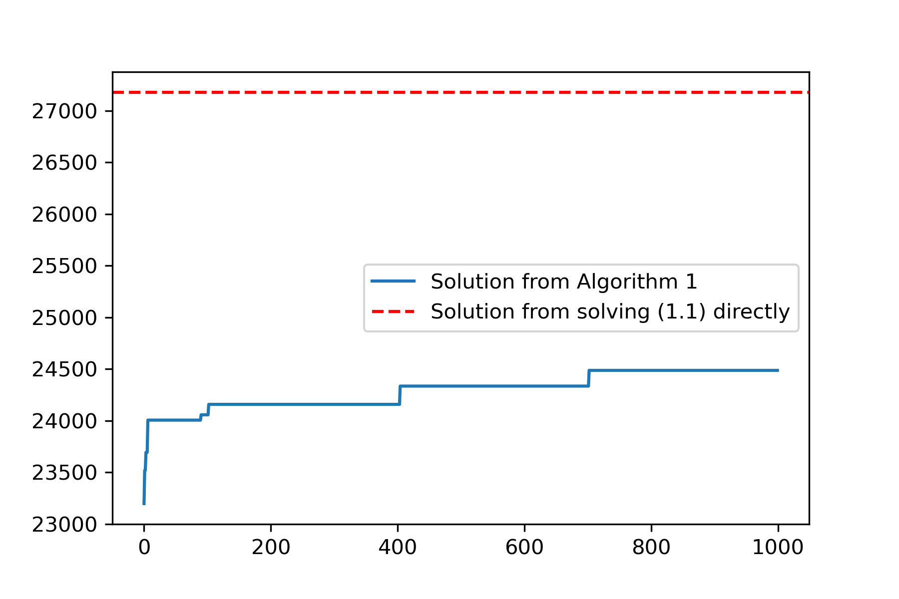
(a) The 600-bus experiment, with an approximation ratio of $90.1\%$.

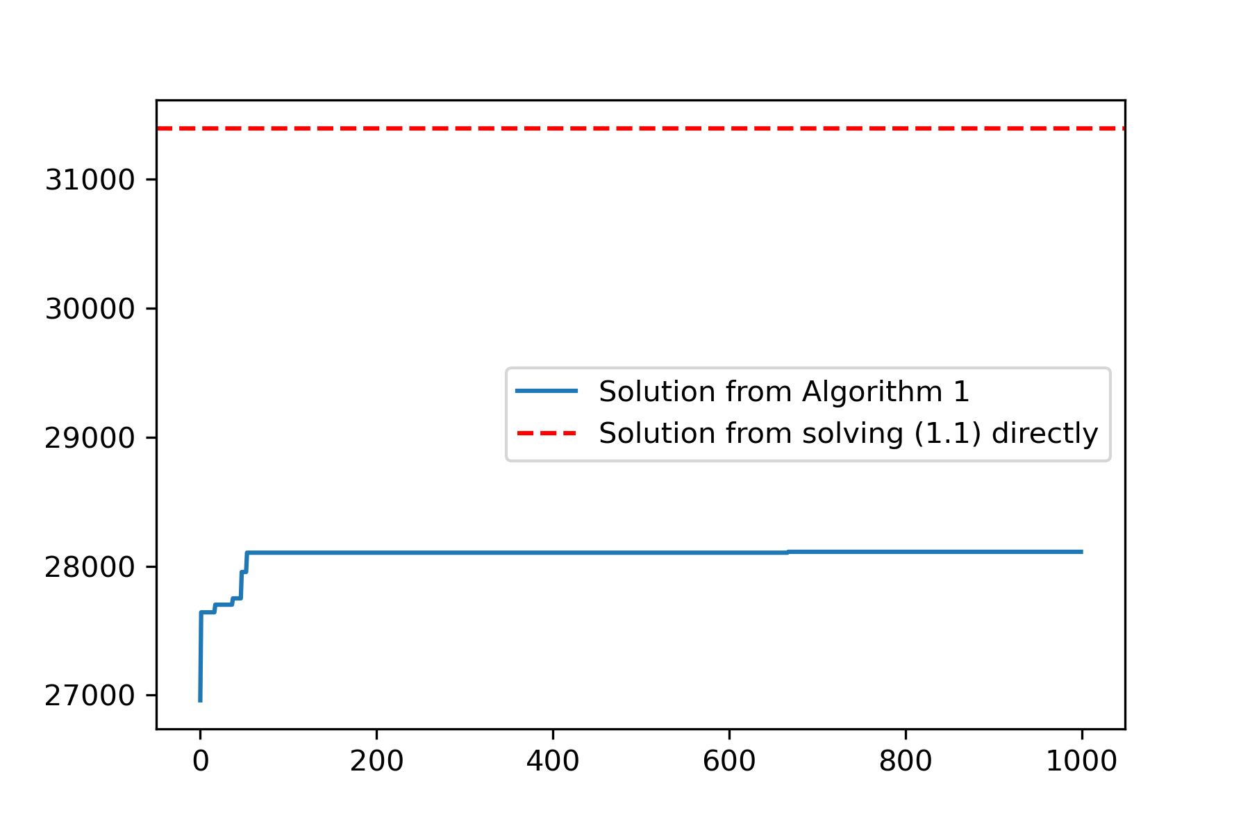
(b) The 800-bus experiment, with an approximation ratio of $89.5\%$.

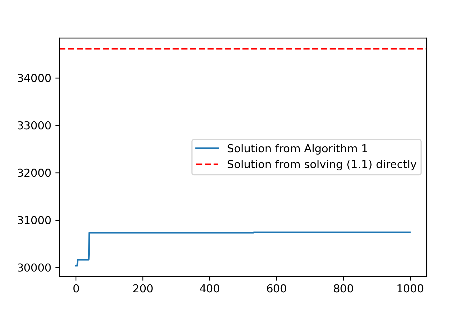
(c) The 1000-bus experiment, with an approximation ratio of $88.8\%$.

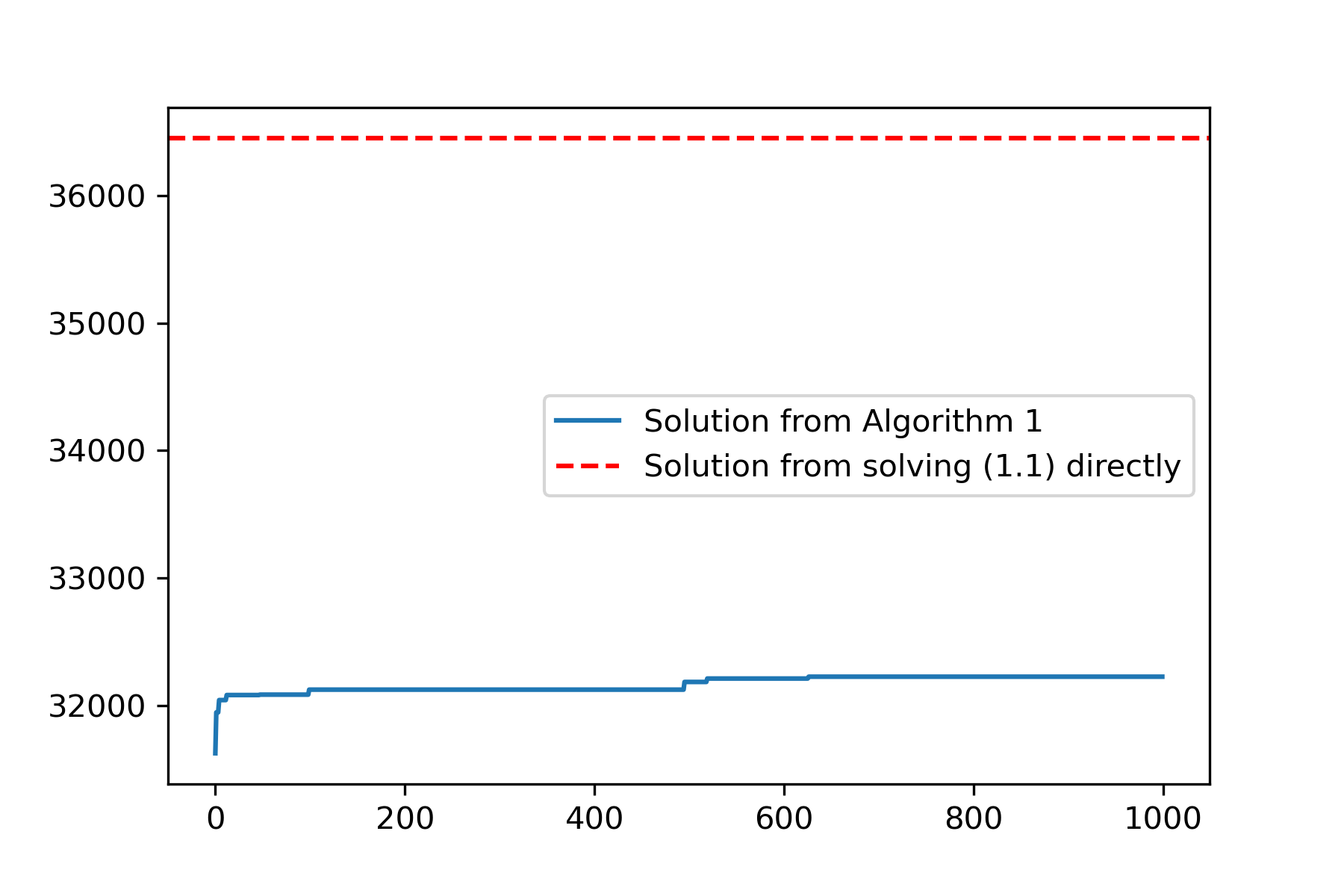
(d) The 1200-bus experiment, with an approximation ratio of $88.4\%$.

Figure 3: Results of four experiments

References

- [1] Igor Averbakh. Probabilistic properties of the dual structure of the multidimensional knapsack problem and fast statistically efficient algorithms. Mathematical Programming, 65(1-3):311–330, 1994.
- [2] Dimitris Bertsimas, Yee Sian Ng, and Julia Yan. Data-driven transit network design at scale. Operations Research, 69(4):1118–1133, 2021.
- [3] Chandra Chekuri, Jan Vondrák, and Rico Zenklusen. Submodular function maximization via the multilinear relaxation and contention resolution schemes. SIAM Journal on Computing, 43(6):1831–1879, 2014.
- [4] Salman Fadaei, MohammadAmin Fazli, and MohammadAli Safari. Maximizing non-monotone submodular set functions subject to different constraints: Combined algorithms. Operations research letters, 39(6):447–451, 2011.
- [5] Uriel Feige. A threshold of for approximating set cover. Journal of the ACM (JACM), 45(4):634–652, 1998.
- [6] Moran Feldman, Joseph Naor, and Roy Schwartz. A unified continuous greedy algorithm for submodular maximization. In 2011 IEEE 52nd annual symposium on foundations of computer science, pages 570–579. IEEE, 2011.
- [7] Lisa Fleischer, Michel X Goemans, Vahab S Mirrokni, and Maxim Sviridenko. Tight approximation algorithms for maximum separable assignment problems. Mathematics of Operations Research, 36(3):416–431, 2011.
- [8] Delbert Fulkerson and Oliver Gross. Incidence matrices and interval graphs. Pacific journal of mathematics, 15(3):835–855, 1965.
- [9] Hongyi Jiang and Samitha Samaranayake. Approximation algorithms for capacitated assignment with budget constraints and applications in transportation systems. In International Computing and Combinatorics Conference (COCOON), pages 94–105. Springer, 2022.
- [10] Ariel Kulik, Hadas Shachnai, and Tami Tamir. Maximizing submodular set functions subject to multiple linear constraints. In Proceedings of the twentieth annual ACM-SIAM symposium on Discrete algorithms, pages 545–554. SIAM, 2009.
- [11] Ariel Kulik, Hadas Shachnai, and Tami Tamir. Approximations for monotone and nonmonotone submodular maximization with knapsack constraints. Mathematics of Operations Research, 38(4):729–739, 2013.
- [12] Jon Lee, Vahab S Mirrokni, Viswanath Nagarajan, and Maxim Sviridenko. Non-monotone submodular maximization under matroid and knapsack constraints. In Proceedings of the forty-first annual ACM symposium on Theory of computing, pages 323–332, 2009.
- [13] Massachusetts Bay Transit Authority. GTFS developers. Accessed August 2, 2018, 2014.
- [14] Rajeev Motwani and Prabhakar Raghavan. Randomized algorithms. Cambridge university press, 1995.
- [15] Noémie Périvier, Chamsi Hssaine, Samitha Samaranayake, and Siddhartha Banerjee. Real-time approximate routing for smart transit systems. Proceedings of the ACM on Measurement and Analysis of Computing Systems, 5(2):1–30, 2021.
- [16] Anita Schöbel. Line planning in public transportation: models and methods. OR spectrum, 34(3):491–510, 2012.
- [17] Lionel Adrian Silman, Zeev Barzily, and Ury Passy. Planning the route system for urban buses. Computers & operations research, 1(2):201–211, 1974.