Joint Problems in Learning Multiple Dynamical Systems

Abstract

Clustering of time series is a well-studied problem, with applications ranging from quantitative, personalized models of metabolism obtained from metabolite concentrations to state discrimination in quantum information theory. We consider a variant, where given a set of trajectories and a number of parts, we jointly partition the set of trajectories and learn linear dynamical system (LDS) models for each part, so as to minimize the maximum error across all the models. We present globally convergent methods and EM heuristics, accompanied by promising computational results.

1 Introduction

Clustering of time series is a well-studied problem [1, 2], with applications ranging from studying mobility patterns [3] to improving Apple Maps [4], through quantitative, personalized models of metabolism obtained from metabolite concentrations, all the way to state discrimination problems in quantum information theory [5].

We consider a variant, where given a set of trajectories and a number of parts, we jointly partition the set of trajectories and learn the autonomous discrete-time Linear Dynamical System (LDS) [6] models:

$$\phi_{t} =\mathbf{G}\phi_{t-1}+\textrm{normally distributed noise},$$ (1)

$$x_{t} =\mathbf{F^{\prime}}\phi_{t}+\textrm{normally distributed noise},$$

for each cluster, where $\phi_{t}$ are the hidden states and $x_{t}$ are the observations. The cluster-specific LDSs may exhibit similar behaviors in terms of system matrices $\mathbf{F},\mathbf{G}$, or not. The observations convey information about the cluster-specific LDSs.

The main contributions of this paper are the following.

• We propose a novel problem in the clustering time-series considering Linear Dynamic System [6] models for each cluster. The linearity assumption comes without a loss of generality as any non-linear system can be modeled as an LDS [7], in a sufficiently higher dimension.

• We provide an abstract formulation within Non-Commutative Polynomial Optimization (NCPOP). NCPOP [8] is a framework for operator-valued optimization problems, and thus does not require the dimension of the hidden state to be known ahead of time, which had been known [9] to be a major limitation of LDS-based methods. This paper is one of the first applications of NCPOP in machine learning.

• As a complement to the NCPOP formulation, we provide an efficient Expectation-Maximization (EM) procedure [10]. Through iterative measurement of prediction errors and systematic updates to the system matrix, we can effectively identify the per-cluster LDSs and the assignment of time series to clusters.

Considering these contributions together with previous work in this direction, notably [11, 12, 13], one obtains a method that:

• learns temporal dynamics in the data and produces the related, interpretable features, unlike methods relying on deep learning.

• does not make any assumptions about the periodic nature of the time series and can handle multiple time lags within the time series, unlike methods based on Fourier coefficients [14].

• does not make any linear-algebraic assumptions, unlike subspace methods [15, 16] that assume the existence of a subspace, which might not necessarily be true. The assumption that the time series were generated by an LDS does not cause any loss of generality.

• does not make any assumptions about the dimension of the hidden state, unlike previous methods utlizing LDS [11, 9, 17, 13].

• improves upon previously proposed methods based on Fast Fourier Transform (FFT) [14] and Dynamic Time Warping (DTW) [18, 19, 20] in practical experiments of Section 5.

2 Background

This section provides an overview and necessary definitions of the background, problems, and algorithms. To orientate the reader, we summarize the notations that we used in this section as Table 1.

2.1 System Identification and Linear Dynamic Systems (LDS)

There is a long history of work in system identification [21] and related approaches in Bayesian statistics [6]. Let $n$ be the hidden state dimension and $m$ be the observational dimension. A linear dynamic system (LDS) $\mathbf{L}$ is defined as a quadruple $(\mathbf{G},\mathbf{F},\mathbf{\Sigma}_{H},\mathbf{\Sigma}_{O})$, where $\mathbf{G}$ and $\mathbf{F}$ are system matrices of dimension $n\times n$ and $n\times m$, respectively. $\mathbf{\Sigma}_{H}\in\mathbb{R}^{n\times n}$ and $\mathbf{\Sigma}_{O}\in\mathbb{R}^{m\times m}$ are covariance matrices [6]. Hence, a single realization of the LDS of length $T$, denoted $\mathbf{X}=\{x_{1},x_{2},\ldots,x_{T}\}\in\mathbb{R}^{m\times T}$, is called a trajectory, and is defined by initial conditions $\phi_{0}$, and realization of noises $\upsilon_{t}$ and $\omega_{t}$ as

$$\phi_{t} =\mathbf{G}\phi_{t-1}+\omega_{t},$$ (2)

$$x_{t} =\mathbf{F}^{\prime}\phi_{t}+\upsilon_{t},$$ (3)

where $\phi_{t}\in\mathbb{R}^{n}$ is the vector autoregressive processes with hidden components and $\left\{\omega_{t},\upsilon_{t}\right\}_{t\in\{1,2,\ldots,T\}}$ are normally distributed process and observation noises with zero mean and covariance of $\mathbf{\Sigma}_{H}$ and $\mathbf{\Sigma}_{O}$ respectively, i.e., $\omega_{t}\sim N(0,\mathbf{\Sigma}_{H})$ and $\upsilon_{t}\sim N(0,\mathbf{\Sigma}_{O})$. The transpose of $\mathbf{F}$ is denoted as $\mathbf{F}^{\prime}$. Vector $x_{t}\in\mathbb{R}^{m}$ serves as an observed output of the system. Recently, Zhou and Marecek [22] proposed to find the global optimum of the objective function subject to the feasibility constraints arising from (2) and (3):

$$\min_{f_{t},\phi_{t},\mathbf{G},\mathbf{F},\omega_{t},\upsilon_{t}}\sum_{t\in\{1,2,\ldots,T\}}\|X_{t}-f_{t}\|_{2}^{2}+\|\omega_{t}\|_{2}^{2}+\|\upsilon_{t}\|_{2}^{2},$$ (4)

for a $L_{2}$-norm $\|\cdot\|_{2}$. In the joint problem we are given $N$ trajectories $\mathbf{X}\in\mathbb{R}^{m\times T}$. A natural problem to solve is to find the parameters of the LDS that generated the trajectories. In other words, we are interested in finding the optimal objective values, as well as system matrices $\mathbf{G},\mathbf{F}$, and the noise vectors $\upsilon_{t}$, $\omega_{t}$ that belong to each LDS.

One should like to remark that learning the LDS is an NP-Hard problem. This is easy to see when one realizes [23] that Gaussian mixture models (GMM), autoregressive models, and hidden Markov models are all special cases of LDS, and whose learning is all NP-Hard, even in very special cases such as spherical Gaussians [24] in a GMM. Furthermore, there are also inapproximability results [24] suggesting that there exists an approximation ratio, at which no polynomial-time algorithm is possible unless P = NP.

Table 1: A Table of Notation.

Symbol	Representation
$i$	Trajectory index
$\mathbf{X}^{i}$	Observation for a trajectory
$t$	Time index
$T$	Length of a trajectory
$K$	Number of clusters
$N$	Number of trajectories
$\phi_{t}$	Hidden state processes
$f_{t}$	Optimal trajectory estimates
$\omega_{t}$	Hidden state noises
$\upsilon_{t}$	Observation error
$n$	Hidden state dimension
$m$	Observational dimension
$\mathbf{L}$	LDS systems specified on $(\mathbf{G},\mathbf{F},\mathbf{\Sigma}_{H},\mathbf{\Sigma}_{O})$
$\mathbf{G}$	System matrix
$\mathbf{F}$	System matrix
$\mathbf{\Sigma}_{H}$	Hidden state noises covariance matrix
$\mathbf{\Sigma}_{O}$	Observation error covariance matrix
$l_{i}$	Assignment of the trajectory $i$
$f^{l_{i}}_{t}$	Optimal trajectory estimates on ${l_{i}}$
$c$	Cluser index
$C_{c}$	Set of trajectories assigned to c
$\mathbf{L_{c}}$	LDS systems generated by $C_{c}$
$\mathbf{G}_{c}$	System matrix of $\mathbf{L_{c}}$
$\mathbf{F}_{c}$	System matrix of $\mathbf{L_{c}}$
$\mathbf{\Sigma}_{H}^{c}$	Hidden covariance matrix of $\mathbf{L_{c}}$
$\mathbf{\Sigma}_{O}^{c}$	Observation covariance matrix of $\mathbf{L_{c}}$
$\phi_{t}^{c}$	Hidden state processes of $\mathbf{L_{c}}$
$\omega_{t}^{c}$	Hidden state noises produced by $\mathbf{L_{c}}$
$\upsilon_{t}^{c}$	Observation error produced by $\mathbf{L_{c}}$

2.2 Clustering with LDS Assumptions

The problem of clustering of time series is relevant in many fields, including [25, 26] applications in Bioinformatics, Multimedia, Robotics, Climate, and Finance. There are a variety of existing methods, including those based on (Fast) Discrete Fourier Transforms (FFTs), Wavelet Transforms, Discrete Cosine Transformations, Singular Value Decomposition, Levenshtein distance, and Dynamic Time Warping (DTW). We compare our method with the FFT- and DTW-based methods below.

There are a number of methods that combine the ideas of system identification and clustering, sometimes providing tools for clustering time series generated by LDSs, similar to our paper. With three related papers at ICML 2023, perhaps this could even be seen as a hot topic. We stress that neither of the papers has formulated the problem as either a mixed-integer program or an NCPOP, or attempted to solve the joint problem without decomposition into multiple steps, which necessarily restricts both the quality of the solutions one can obtain in practice, as well as the strength of the guarantees that can be obtained in theory.

To our knowledge, the first mention of clustering with LDS assumptions is in the paper of [11], who introduced ComplexFit, a novel EM algorithm to learn the parameters for complex-valued LDSs and utilized it in clustering. In [9], regularization has been used in learning linear dynamical systems for multivariate time series analysis. In a little-known but excellent paper at AISTATS 2021, Hsu et al. [12] consider clustering with LDS assumptions, but argue for clustering on the eigenspectrum of the state-transition matrix ($\mathbf{G}$ in our notation), which can be identified for unknown linear dynamics without full system identification. The main technical contribution is bidirectional perturbation bounds to prove that two LDSs have similar eigenvalues if and only if their output time series have similar parameters within Autoregressive-Moving-Average (ARMA) models. Standard consistent estimators for the autoregressive model parameters of the ARMA models are then used to estimate the LDS eigenvalues, allowing for linear-time algorithms. We stress that the eigenvalues may not be interpretable as features; one has to provide the dimension of the hidden state as an input.

At ICML 2023, Bakshi et al. [17] presented an algorithm to learn a mixture of linear dynamic systems. Each trajectory is generated so that an LDS is selected on the basis of the weights of the mixture, and then a trajectory is drawn from the LDS. Their approach is, unlike ours, based on moments and the Ho-Kalman algorithm and tensor decomposition, which is generalized to work with the mixture. Empirically, [17] outperforms the previous work of Chen et al. [27] of the previous year, which works in fully observable settings. In the first step, the latter algorithm [17] finds subspaces that separate the trajectories. In the second step, a similarity matrix is calculated, which is then used in clustering and consequently can be used to estimate the model parameters. The paper [17] also discusses the possibility of classification of new trajectories and provides guarantees on the error of the final clustering.

Also at ICML 2023, [28] presented learning of mixtures of Hidden Markov Models and Markov Chains. The method estimates subspaces first, then uses spectral clustering and MDP transition matrices estimation step followed by the possibility to classify new trajectories. The paper provides performance guarantees for each step.

Still at the same conference, [29] consider the learning of a single LDS across all trajectories and fine-tuning the target policy for some subsets thereof. The main contribution of [29] is a bound on the imitation gap over trajectories generated by the learned target policy.

Finally, there is a notable arxiv pre-print. A joint problem related to [29] is being considered by [13], who propose to jointly estimate transition matrices of multiple linear time-invariant dynamic systems, where the transition matrices are all linear functions of some shared unknown base matrix. Also, as opposed to our method, the state of the system is assumed to be fully observable.

There are also first applications of the joint problems in the domain-specific literature. Similarly to the previous paper, a fully observable setting of vector autoregressive models is considered in [30], with applications in Psychology, namely on depression-related symptoms of young women. Similarly to our method, the least-squares objective is minimized to provide clustering in a manner similar to the EM-heuristic. See also [31] for further applications in Psychology. One can easily envision a number of further uses across Psychology and Neuroscience, especially when the use of mixed-integer programming solvers simplifies the time-consuming implementation of EM algorithms.

2.3 Mixed-Integer Programming (MIP)

To search for global optima, we developed relaxations to bound the optimal objective values in non-convex Mixed-Integer Nonlinear Programs (MINLPs) [32]. Our study is based on the Mixed-Integer Nonlinear Programs of the form:

$$\min f(x,y,z)$$ (MINLP)

$$\textrm{s.t. }g_{i}(x,y,z)\leq 0, \quad\forall i\in I,$$ (5)

$$h_{j}(x)\leq 0, \quad\text{if }z_{j}=1,\forall j\in J,$$ (6)

$$\quad x\in\mathbb{R}^{n},y\in\mathbb{Z}^{m}$$

where functions $f$, $g_{i}$ and $h_{j}$ are assumed to be continuous and twice differentiable. Such problems are non-convex, both in terms of featuring integer variables and in terms of the functions $f,g_{i}$.

While MINLP problems may seem too general a model for our joint problem, notice that the NP-hardness and inapproximability results discussed in Section 2.1 suggest that this may be the appropriate framework. For bounded variables, standard branch-and-bound-and-cut algorithms run in finite time. Both in theory – albeit under restrictive assumptions, such as in [33] – and in practice, the expected runtime is often polynomial. In the formulation of the next section, $f,g_{i}$ are trilinear, and various monomial envelopes have been considered and implemented in global optimization solvers such as BARON [34], SCIP [35], and Gurobi. In our approach, we consider a mixed-integer programming formulation of a piecewise polyhedral relaxation of a multilinear term using its convex-hull representation.

2.4 Non-Commutative Polynomial Optimization (NCPOP)

To extend the search for global optima from a fixed finite-dimensional state to an operator in an unknown dimension, we formulate the problem as a non-commutative polynomial optimization problem (NCPOP), cf. [36] . Our study is based on NCPOP: (H,X,ψ) ⟨ψ,p(X)ψ⟩P^*= q_i(X)≽0, i=1,…,m ⟨ψ,ψ⟩= 1, where $X=(X_{1},\ldots,X_{n})$ is a tuple of bounded operators on a Hilbert space $\mathcal{H}$. In contrast to traditional scalar-valued, vector-valued, or matrix-valued optimization techniques, the dimension of variables $X$ is unknown a priori. Let $[X,X^{{\dagger}}]$ denotes these $2n$ operators, with the ${\dagger}$-algebra being conjugate transpose. The normalized vector $\psi$, i.e., $\|\psi\|^{2}=1$ is also defined on $\mathcal{H}$ with the inner product $\langle\psi,\psi\rangle=1$. $p(X)$ and $q_{i}(X)$ are polynomials and $q_{i}(X)\succcurlyeq 0$ denotes that the operator $q_{i}(X)$ is positive semidefinite. Polynomials $p(X)$ and $q_{i}(X)$ of degrees $\deg(p)$ and $\deg(q_{i})$, respectively, can be written as:

$$p(X)=\sum_{|\omega|\leq\deg(p)}p_{\omega}\omega,\quad q_{i}(X)=\sum_{|\mu|\leq\deg(q_{i})}q_{i,\mu}\mu,$$ (7)

where $i=1,\ldots,m$ and $\deg(p)$ refers to the polynomial degree of $p$. Monomials $\omega,\mu,u$ and $\nu$ in following text are products of powers of variables from $[X,X^{{\dagger}}]$. The degree of a monomial, denoted by $|\omega|$, refers to the sum of the exponents of all operators in the monomial $\omega$. Let $\mathcal{W}_{k}$ denote the collection of all monomials whose degrees $|\omega|\leq k$, or less than infinity if not specified. If $(\mathcal{H},X,\psi)$ is feasible, one can utilize the Sums of Squares theorem of [37] and [38] to derive semidefinite programming (SDP) relaxations of the Navascules-Pironio-Acin (NPA) hierarchy [39, 40]. There are also variants [41, 42, 43] that exploit various forms of sparsity.

3 Problem Formulation

Suppose that we have $N$ trajectories denoted by $\mathbf{X}^{i}\in\mathbb{R}^{m\times T}$ for $i\in\{1,2,\ldots,N\}$. We assume that those trajectories were from $K(=2)$ clusters, $C_{0}$ and $C_{1}$. The trajectory of the cluster $C_{0}$ (resp. $C_{1}$) was generated by a LDS $\mathbf{L_{0}}$ (resp. $\mathbf{L_{1}}$). We aim to jointly partition the given set of trajectories into $K(=2)$ clusters and recover the parameters of the LDSs systems of both clusters $C_{0},C_{1}$. To solve these joint optimization problems, we can introduce an indicator function to determine how the $N$ trajectories are assigned to two clusters:

$$l_{i}=\begin{cases}0,&\text{if}\ i\in C_{0},\\ 1,&\text{if}\ i\in C_{1},\end{cases}$$ (8)

for $i\in\{1,2,\ldots,N\}$.

3.1 Least-Squares Objective Function

We define the optimization problem with a least-squares objective that minimizes the difference of measurement estimates $f^{0}_{t}\in\mathbb{R}^{n\times T}$, $f^{1}_{t}\in\mathbb{R}^{n\times T}$ and the corresponding measurements. Other variables include noise vectors that come with the estimates, indicator function $l_{i}$ that assigns the trajectories to the clusters, and parameters of systems $\mathbf{L_{0}}$ and $\mathbf{L_{1}}$ (also known as system matrices). The objective function reads:

$$\min_{\begin{subarray}{c}f^{0}_{t},\mathbf{F}_{0},\mathbf{G}_{0},\upsilon^{0}_{t},\omega^{0}_{t},\phi_{0}^{0},\\ f^{1}_{t},\mathbf{F}_{1},\mathbf{G}_{1},\upsilon^{1}_{t},\omega^{1}_{t},\phi_{0}^{1}\\ l_{i}\end{subarray}}\sum_{i=1}^{N}\sum_{t=1}^{T}\|X^{i}_{t}-f^{l_{i}}_{t}\|_{2}^{2}\\ +\sum_{c\in\{0,1\}}\sum_{t=1}^{T}\left[\|\upsilon_{t}^{c}\|_{2}^{2}+\|\omega_{t}^{c}\|_{2}^{2}\right]\\ \omega_{t}^{c}\sim N(0,\mathbf{\Sigma}_{H}^{c}),\upsilon_{t}^{c}\sim N(0,\mathbf{\Sigma}_{O}^{c}),$$ (9)

where $\upsilon^{c},\omega^{c}$ are defined above and $\|\cdot\|_{2}$ denotes the $L_{2}$ norm. Note that the indicator index $l_{i}$ in the superscript in (9) can be replaced by multiplication with the indicator function, i.e.,

$$\|X^{i}_{t}-f^{l_{i}}_{t}\|_{2}^{2}=\|X^{i}_{t}-f^{0}_{t}\|_{2}^{2}\cdot(1-l_{i})+\|X^{i}_{t}-f^{1}_{t}\|_{2}^{2}\cdot l_{i}.$$ (10)

In the first part of the optimization criterion (9), we have a sum of squares of the difference between trajectory estimate $f_{t}^{l_{i}}$ and observations of the trajectories assigned to cluster $C_{c}$ for $c=0,1$. The second part of the optimization criterion (10) provides a form of regularization.

3.2 Feasible Set in State Space

The feasible set given by constraints is as follows:

$$\phi^{c}_{t} =\mathbf{G}_{c}\phi^{c}_{t-1}+\omega^{c}_{t}, \forall t=2,\dots,T, \forall c=0,1,$$ (11)

$$f^{c}_{t} =\mathbf{F}^{{}^{\prime}}_{c}\phi^{c}_{t}+\upsilon^{c}_{t}, \forall t=1,\dots,T, \forall c=0,1,$$ (12)

$$l_{i}^{2} =l_{i} \forall i=1,\dots,N.$$ (13)

The first two equations in the set of constraints, (11) and (12), encode that the system is an LDS with system matrices $\mathbf{F}$ and $\mathbf{G}$. For brevity of the notation, both equations are indexed by the cluster index $c$, which can be rewritten as twice as many equations, one with $f^{0}_{t},\mathbf{F}_{0},\mathbf{G}_{0},\upsilon^{0}_{t},\omega^{0}_{t}$, and $\phi_{t}^{0}$, the second one with $f^{1}_{t},\mathbf{F}_{1},\mathbf{G}_{1},\upsilon^{1}_{t},\omega^{1}_{t}$, and $\phi_{t}^{1}$. The third equation (13) encodes that the indicator function is $0$ or $1$ for each trajectory.

We can also add redundant constraints for all $i=1,2,\ldots,N$:

$$l_{i}\phi^{1}_{t} =l_{i}(\mathbf{G}_{1}\phi^{1}_{t-1}+\omega^{1}_{t}), \forall t=2,\dots,T,$$

$$l_{i}f^{1}_{t} =l_{i}(\mathbf{F}^{{}^{\prime}}_{1}\phi^{1}_{t}+\upsilon^{1}_{t}), \forall t=1,\dots,T,$$

$$(1-l_{i})\phi^{0}_{t} =(1-l_{i})(\mathbf{G}_{0}\phi^{0}_{t-1}+\omega^{0}_{t}), \forall t=2,\dots,T,$$

$$(1-l_{i})f^{0}_{t} =(1-l_{i})(\mathbf{F}^{{}^{\prime}}_{0}\phi^{l}_{t}+\upsilon^{0}_{t}), \forall t=1,\dots,T,$$

or even a weighted combination of the redundant constraints in the spirit of Gomory. While these strengthen the relaxations, the higher-degree polynomials involved come at a considerable cost.

3.3 Variants and Guarantees

There are several variants of the formulation above. Clearly, one can:

• consider a fixed, finite dimension of the hidden state $\phi$ to be known and to solve a finite-dimensional (MINLP) – or to consider the dimension to be unknown and to solve an operator-valued problem as in Zhou and Marecek [22].

• consider side constraints on the system matrices $\mathbf{F},\mathbf{G}$, as in Ahmadi and El Khadir [44] – or not. At least requiring the norm of $\mathbf{G}$ to be 1 is without loss of generality.

• bound the magnitude of the process noise $\omega^{c}$ and observation noise $\upsilon^{c}$, or other shape constraints thereupon – or not.

• bound the cardinality of the clusters – or not.

Throughout, one obtains asymptotic guarantees on the convergence of the NCPOP, or guarantees of finite convergence in the case of the MINLP.

4 EM Heuristic

In addition to tackling the optimization problem in Section 3.1, we provide an alternative solver using the Expectation-Maximization (EM) heuristic [10]. The main idea of the algorithm is to avoid the direct optimization of the criterion in (9). Instead, the indicator function is treated separately. In the expectation step, the parameters of the LDSs are fixed, and the assignment of the trajectories to the clusters (i.e., the indicator function) is calculated. Then, in the maximization step, the criterion is optimized, and the LDS parameters are calculated with the indicator function fixed. See Algorithm 1 for the pseudocode. First, the algorithm randomly partitions the trajectories into the clusters. Then, for each cluster, the parameters of the LDSs are found, and with the parameters known, the optimization criterion is recalculated, and each trajectory is put to the cluster, which lowers the error in (9).

The advantage is that the problem of finding the parameters and an optimal trajectory for a set of trajectories is easier than clustering the trajectories. The problem was already studied in [22]. Another advantage of the EM heuristic is that it can be easily generalized to an arbitrary number of clusters $K$, generally for any $K>1$.

function EM-clustering($N$ trajectories $\mathbf{X}^{i}\in\mathbb{R}^{m\times T}$, $K$)

     $\triangleright$ Generate a random partitioning into two clusters.

     $l_{i}\leftarrow\textsc{RandomInt}(\{0,1,\ldots,K-1\})$

     

     $\triangleright$ Iterate until convergence.

     while $l_{i}$ changes for any $i\in\{1,2,\ldots,N\}$ do

         $\triangleright$ For each cluster find cluster parameters

         for $c\in\{0,1,\ldots,K\}$ do

              Find the cluster $C_{c}$ parameters by solving

$$\min_{\begin{subarray}{c}f^{c}_{t},\mathbf{F}_{c},\mathbf{G}_{c},\upsilon^{c}_{t},\omega^{c}_{t},\phi_{c}^{0}\end{subarray}}\left[\sum_{i=1}^{N}\sum_{t=1}^{T}\|X^{i}_{t}-f^{c}_{t}\|_{2}^{2}\right]+\|\upsilon^{c}\|_{2}^{2}+\|\omega^{c}\|_{2}^{2}$$

         end for

         

         $\triangleright$ Reassign the trajectories to the clusters.

         for $i\in\{1,2,\ldots N\}$ do

              $l_{i}\leftarrow\displaystyle\mathop{\mathrm{arg\,min}}_{c\in\{0,1,\ldots,K-1\}}\sum_{t=1}^{T}\|X^{i}_{t}-f^{c}_{t}\|_{2}^{2}$

         end for

     end while

end function

Algorithm 1 The EM heuristic.

5 Experiments

In this section, we present a comprehensive set of experiments to evaluate the effectiveness of the proposed (MINLP) and EM heuristic, without considering any side constraints and without any shape constraints. Our experiments are conducted on Google Colab with two Intel(R) Xeon(R) (2.20GHz) CPUs and Ubuntu 22.04. The source code is included in the Supplementary Material.

5.1 Methods and Solvers

MIP-IF

Our formulation for MIP-IF uses equations (10) subject to (11–13). We specify the dimensions of system matrices, i.e., $n$ and $m$ as hyperparameters. For every data set, we perform $50$ experiments, in which different random seeds are employed to initialize the indicator function in each iteration. These MIP instances are solved via Bonmin [45].

EM Heuristic

Iterated EM Heuristic clustering is presented in Algorithm 1. As in MIP-IF, dimensions of system matrices $n$ and $m$ are required. In each iteration, the cluster partition is randomly initialized and we conduct $50$ trials with various random seeds for every dataset.

The discussion of runtime As a subroutine of the EM Heuristic, the LDS identification in equation (9) is solved via Bonmin, with runtime presented in the right subplot of Figure 3. When the dimensions of system matrices are not assumed, the LDS identification becomes an NCPOP, and the runtime increase exponentially if using NPA hierarchy [39, 40] is used to find the global optimal solutions, but stay relatively modest if sparity exploit variants [41, 42, 43] are used.

Baselines

We consider the following traditional time series clustering methods as baselines:

• Dynamic Time Warping (DTW) is used for measuring similarity between given time series [18, 19]. We utilize K-means on DTW distance with tslearn [46] package.

• Fast Fourier Transform (FFT) is utilized to obtain the Fourier coefficients and the distance between time series is evaluated as the L2-norm of the difference in their respective Fourier coefficients. Subsequently, K-means is employed to cluster time series using this distance.

5.2 Clustering Performance Metrics

The $F_{1}$ score, which has been widely used in classification performance measurements, is defined as

$$F_{1}=2\cdot\frac{\textrm{precision}\cdot\textrm{recall}}{\textrm{precision}+\textrm{recall}}$$ (14)

where precision $=\frac{TP}{TP+FP}$ and recall $=\frac{TP}{TP+FN}$ and $TP$, $FP$, and $FN$ are the numbers of true positives, false positives, and false negatives, respectively. We calculate the $F_{1}$ score twice for each class, once with one class labeled as positive and once with the other class labeled as positive, and then we select the higher score for each class. This approach is used because there is no predefined positive and negative labels.

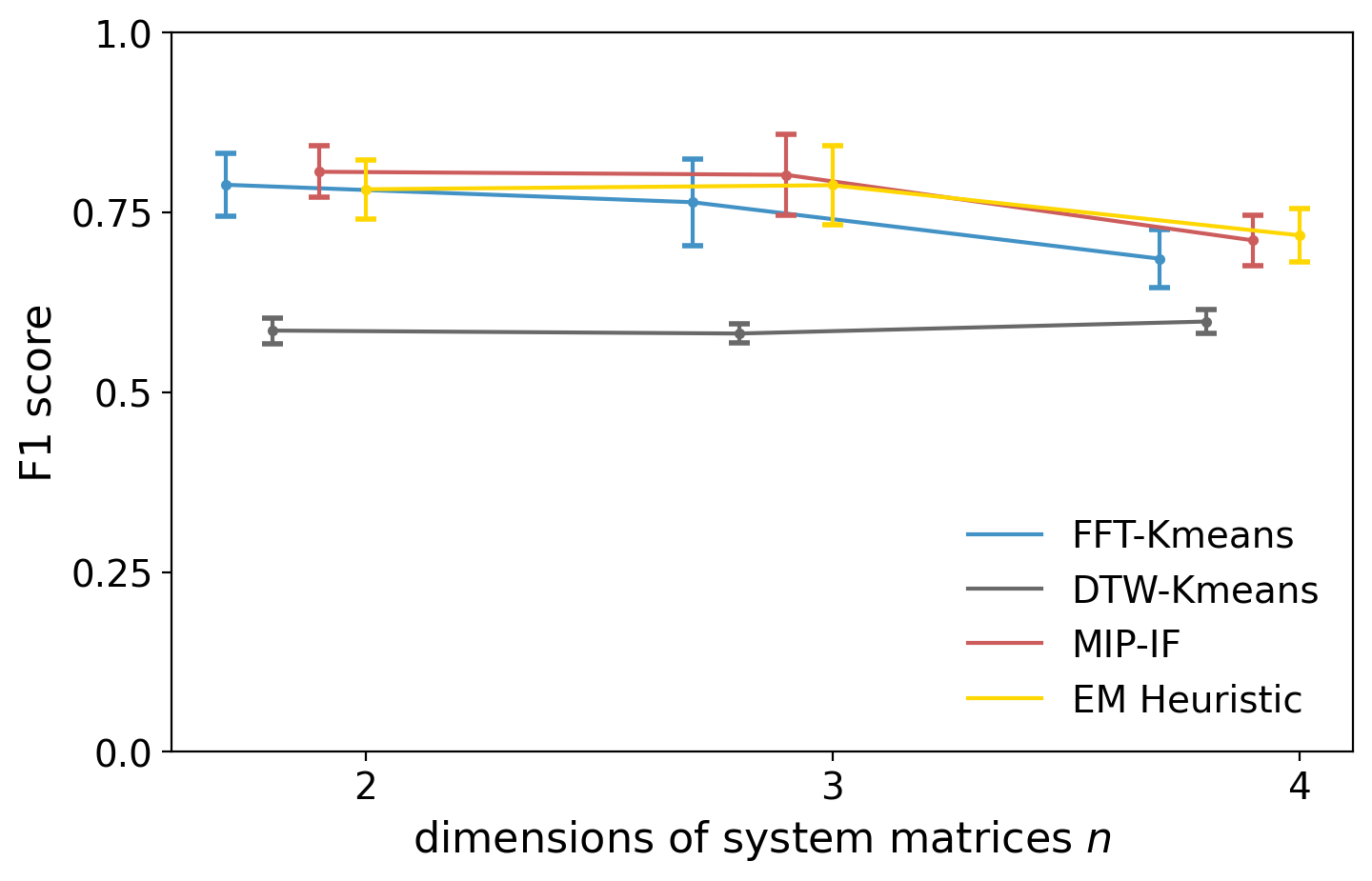
Figure 1: $F_{1}$ scores of proposed methods compared to baselines. The results are based on the data generated by LDSs with hidden state dimensions $n\in\{2,3,4\}$ respectively. The vertical error bars show the $95\%$ confidence intervals of the $50$ trials. A higher $F_{1}$ score indicates better clustering performance.

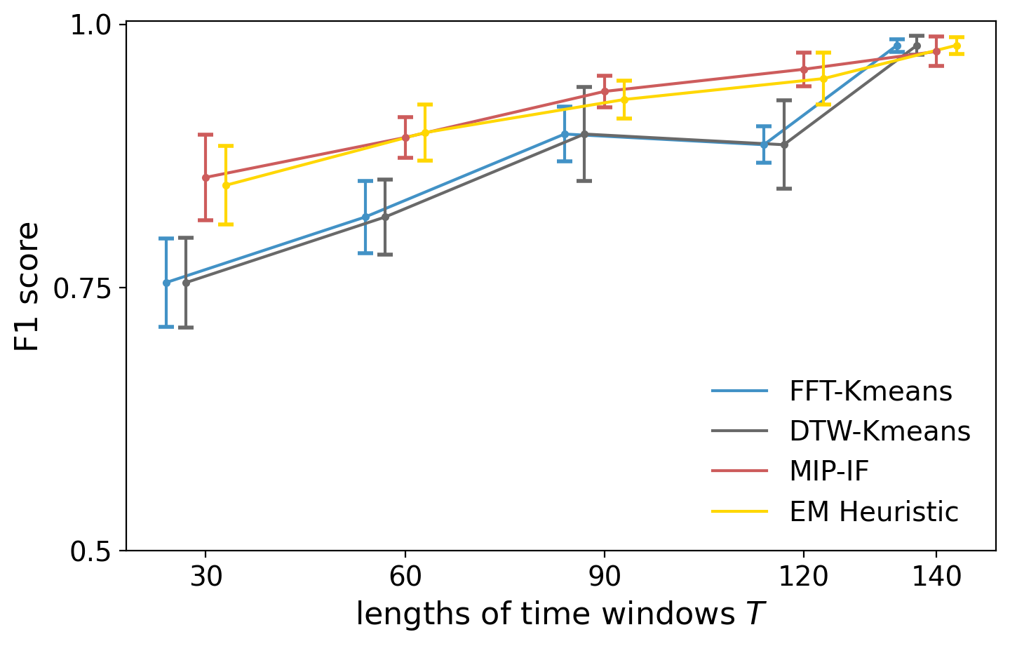
Figure 2: $F_{1}$ scores of proposed methods compared to baselines. The results are based on data sampled from ECG5000 with various time window $T$ chosen from $\{30,60,90,120,140\}$. For MIP-IF and EM Heuristic, $F_{1}$ scores are generated with hidden state dimension $n=3$. A higher $F_{1}$ score indicates better clustering performance.

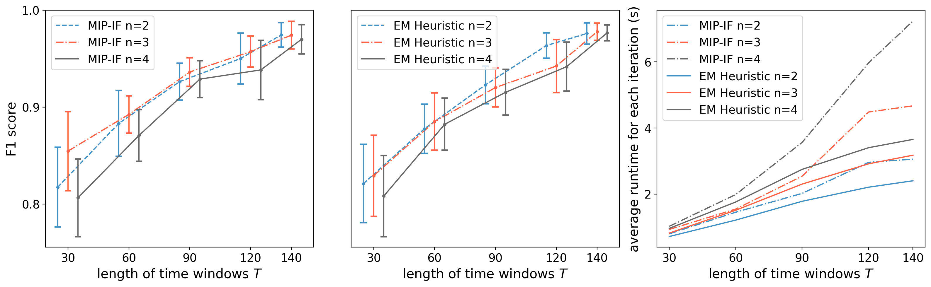
Figure 3: Left and Center: $F_{1}$ scores of MIP-IF and EM Heuristic with various hidden state dimension $n$ chosen from $\{2,3,4\}$ respectively. Right: Runtime of these two methods under distinct settings.

5.3 Experiments on Synthetic Data

Data Generation

We generate LDSs by specifying the quadruple $(\mathbf{G},\mathbf{F},\mathbf{\Sigma}_{H},\mathbf{\Sigma}_{O})$ and the initial hidden state $\phi_{0}$. $\mathbf{G}$ and $\mathbf{F}$ are system matrices of dimensions $n\times n$ and $n\times m$, respectively. For each cluster, we derive $\frac{N}{2}$ trajectories including $T$ observations. The dimension $m$ of the observations is set to $2$ and hidden-state dimension $n$ is chosen from $\{2,3,4\}$. To make these LDSs close to the center of the respective cluster, we fix the system matrices while only changing the covariance matrices $\mathbf{\Sigma}_{H},\mathbf{\Sigma}_{O}$ from $0.0004,0.0016,0.0036$, to $0.0064$ respectively. Note that $\mathbf{\Sigma}_{H}=0.0004$ here refers to $\mathbf{\Sigma}_{H}=0.0004\times\mathbf{I}_{n}$, where $\mathbf{I}_{n}$ is the $n\times n$ identity matrix. We consider all combinations of covariance matrices ($16$ trajectories) for each cluster. Please see the Supplementary Material for details.

Results

In our first simulation, we explore the effectiveness of the proposed methods in synthetic datasets. For each choice of $n\in\{2,3,4\}$, we run $50$ trials. In each trial, the indicator function $l_{i}$ for MIP-IF and the original clustering partition for EM Heuristic are randomly initialized.

Figure 1 illustrates the $F_{1}$ score of our methods and baselines, with $95\%$ confidence intervals from $50$ trials. Different approaches are distinguished by colors: blue for “FFT-Kmeans”, grey for “DTW-Kmeans”, red for “MIP-IF” and yellow for “EM Heuristic”. Both solutions proposed yield superior cluster performance considering $n\in\{3,4\}$. When $n=2$, our methods can achieve comparable performance to FFT-Kmeans. These experiments on synthetic datasets thus demonstrate the effectiveness of our approach.

5.4 Experiments on Real-world Data

Next, we conduct experiments on real-world data.

ECG data

The electrocardiogram (ECG) data ECG5000 [47] is a common dataset for evaluating methods for ECG data, which has also been utilized by also by other papers [12] on clustering with LDS assumptions. The original data comes from Physionet [48, 49] and contains a $20$-hour-long ECG for congestive heart failure. After processing, ECG5000 includes 500 sequences, where there are $292$ normal samples and $208$ samples of four types of heart failure. Each sequence contains a whole period of heartbeat with $140$ time stamps.

Results on ECG

We randomly sample two clusters from normal sequences and one type of abnormal sequences respectively. As the entire period of time series data is not always available, we also extract subsequences with various lengths of time window $T$ chosen from $\{30,60,90,120\}$ to test the clustering performance.

In Figure 2, with the assumption of the hidden state dimension $n=3$, we implement all methods for $50$ runs at each length of time window. Our methods exhibit competitive performance relative to FFT and DTW. When the time window decreases, the performance of the baselines significantly deteriorates, while our methods maintain a higher level of robustness.

In Figure 3, we further explore the performance of our methods at varying dimensions of the hidden state ($n\in\{2,3,4\}$), because the dimension of the hidden state $n$ of the ECG data is, indeed, unknown. The $F_{1}$ scores of MIP-IF and EM Heuristic are presented in the left and center subplots. When the length of the time window increases, both methods experience a slight improvement in clustering performance, but this performance remains relatively stable when the dimension $n$ changes. The runtime is presented in the right subplot. Compared to MIP-IF, the EM Heuristic exhibits a modest growth in runtime as the length of the time window increases.

Finally, when the dimension $n$ of the hidden state is not assumed, the subproblem of the EM heuristic becomes an NCPOP. For the implementation with such an assumption, we construct NCPOP using ncpol2sdpa 1.12.2 [50]. Subsequently, the relaxation problem is solved by Mosek 10.1 [51]. Noted that the execution time of NCPOP escalates rapidly as the trajectory length $T$ grows, we test NCPOP with $T\in\{10,20,30\}$. For comparison, we use pyomo [52] to construct the model and solve the problem with Bonmin [45], as above, with the dimension $n$ from $\{2,3,4\}$. The overall performance of different methods under various settings is illustrated in Figure 4. NCPOP demonstrates the best performance in terms of the $F_{1}$ score when $T=10$ and $30$. The runtime of NCPOP grows significantly as the length $T$ of the trajectory increases.

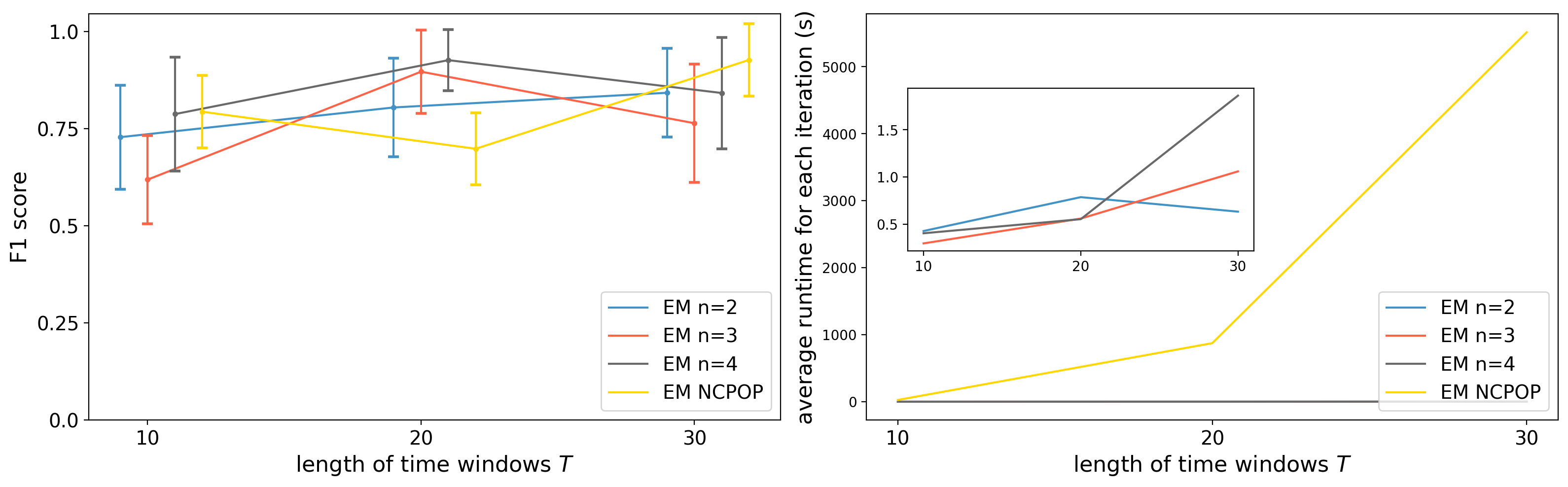
Figure 4: $F_{1}$ scores (left) and runtimes (right) of EM Heuristic using NCPOP compared with the method requiring specific dimension $n$ of hidden state. $n$ is chosen from $\{2,3,4\}$.

6 Conclusions and Further Work

We have studied problems in clustering time series, where given a set of trajectories and a number of parts, we jointly partition the set of trajectories and estimate a linear dynamical system (LDS) model for each part, so as to minimize the maximum error across all the models. As discussed in Section 3.3, a number of variants of the joint problem remain to be investigated. The computational aspects of the operator-valued problem [22] that consider the dimension of the hidden state to be unknown seem particularly interesting. See the supplementary material for further details of the operator-valued problem.

It would be of considerable interest to analyse the behaviour of the EM heuristic in our setting. Indeed, for many problems, such as the parameter estimation of Gaussian mixture models [53, 54], the properties of EM approaches are well understood [53, 55, 54, 56, 57]. The joint problems seem somewhat similar, inasmuch as one could see the joint problem as a parameter estimation of a mixture of Gaussian distribution over the system matrices.

References

- [1] M. Vlachos, G. Kollios, and D. Gunopulos, “Discovering similar multidimensional trajectories,” in Proceedings 18th international conference on data engineering, pp. 673–684, IEEE, 2002.
- [2] E. Keogh, T. Palpanas, V. B. Zordan, D. Gunopulos, and M. Cardle, “Indexing large human-motion databases,” in Proceedings of the Thirtieth international conference on Very large data bases-Volume 30, pp. 780–791, 2004.
- [3] M. Mokbel, M. Sakr, L. Xiong, A. Züfle, J. Almeida, W. Aref, G. Andrienko, N. Andrienko, Y. Cao, S. Chawla, et al., “Towards mobility data science (vision paper),” arXiv preprint arXiv:2307.05717, 2023.
- [4] C. Chen, C. Lu, Q. Huang, Q. Yang, D. Gunopulos, and L. Guibas, “City-scale map creation and updating using gps collections,” in Proceedings of the 22nd ACM SIGKDD International Conference on Knowledge Discovery and Data Mining, pp. 1465–1474, 2016.
- [5] E. Magesan, J. M. Gambetta, A. D. Córcoles, and J. M. Chow, “Machine learning for discriminating quantum measurement trajectories and improving readout,” Physical review letters, vol. 114, no. 20, p. 200501, 2015.
- [6] M. West and J. Harrison, Bayesian forecasting and dynamic models. Springer Science & Business Media, 2006.
- [7] P. Bevanda, S. Sosnowski, and S. Hirche, “Koopman operator dynamical models: Learning, analysis and control,” Annual Reviews in Control, vol. 52, pp. 197–212, 2021.
- [8] S. Pironio, M. Navascués, and A. Acín, “Convergent relaxations of polynomial optimization problems with noncommuting variables,” SIAM Journal on Optimization, vol. 20, no. 5, pp. 2157–2180, 2010.
- [9] Z. Liu and M. Hauskrecht, “A regularized linear dynamical system framework for multivariate time series analysis,” in Proceedings of the AAAI Conference on Artificial Intelligence, vol. 29, 2015.
- [10] A. P. Dempster, N. M. Laird, and D. B. Rubin, “Maximum likelihood from incomplete data via the EM algorithm,” Journal of the Royal Statistical Society. Series B (Methodological), vol. 39, no. 1, pp. 1–38, 1977.
- [11] L. Li and B. A. Prakash, “Time series clustering: Complex is simpler!,” in Proceedings of the 28th International Conference on Machine Learning (ICML-11), pp. 185–192, 2011.
- [12] C. Hsu, M. Hardt, and M. Hardt, “Linear dynamics: Clustering without identification,” in International Conference on Artificial Intelligence and Statistics, pp. 918–929, PMLR, 2020.
- [13] A. Modi, M. K. S. Faradonbeh, A. Tewari, and G. Michailidis, “Joint learning of linear time-invariant dynamical systems,” 2022.
- [14] K. Kalpakis, D. Gada, and V. Puttagunta, “Distance measures for effective clustering of arima time-series,” in Proceedings 2001 IEEE international conference on data mining, pp. 273–280, IEEE, 2001.
- [15] R. Agrawal, J. Gehrke, D. Gunopulos, and P. Raghavan, “Automatic subspace clustering of high dimensional data for data mining applications,” in Proceedings of the 1998 ACM SIGMOD international conference on Management of data, pp. 94–105, 1998.
- [16] C. Domeniconi, D. Papadopoulos, D. Gunopulos, and S. Ma, “Subspace clustering of high dimensional data,” in Proceedings of the 2004 SIAM international conference on data mining, pp. 517–521, SIAM, 2004.
- [17] A. Bakshi, A. Liu, A. Moitra, and M. Yau, “Tensor decompositions meet control theory: Learning general mixtures of linear dynamical systems,” in Proceedings of the 40th International Conference on Machine Learning (A. Krause, E. Brunskill, K. Cho, B. Engelhardt, S. Sabato, and J. Scarlett, eds.), vol. 202 of Proceedings of Machine Learning Research, pp. 1549–1563, PMLR, 23–29 Jul 2023.
- [18] H. Sakoe and S. Chiba, “Dynamic programming algorithm optimization for spoken word recognition,” IEEE transactions on acoustics, speech, and signal processing, vol. 26, no. 1, pp. 43–49, 1978.
- [19] D. Gunopulos and G. Das, “Time series similarity measures and time series indexing,” in SIGMOD Conference, p. 624, 2001.
- [20] M. Shah, J. Grabocka, N. Schilling, M. Wistuba, and L. Schmidt-Thieme, “Learning dtw-shapelets for time-series classification,” in Proceedings of the 3rd IKDD Conference on Data Science, 2016, CODS ’16, (New York, NY, USA), Association for Computing Machinery, 2016.
- [21] L. Ljung, “Perspectives on system identification,” Annual Reviews in Control, vol. 34, no. 1, pp. 1–12, 2010.
- [22] Q. Zhou and J. Mareček, “Learning of linear dynamical systems as a non-commutative polynomial optimization problem,” IEEE Transactions on Automatic Control, 2023.
- [23] S. Roweis and Z. Ghahramani, “A unifying review of linear Gaussian models,” Neural computation, vol. 11, no. 2, pp. 305–345, 1999.
- [24] C. Tosh and S. Dasgupta, “Maximum likelihood estimation for mixtures of spherical Gaussians is NP-hard.,” J. Mach. Learn. Res., vol. 18, pp. 175–1, 2017.
- [25] S. Aghabozorgi, A. Seyed Shirkhorshidi, and T. Ying Wah, “Time-series clustering –- a decade review,” Information Systems, vol. 53, pp. 16–38, 2015.
- [26] T. Warren Liao, “Clustering of time series data – a survey,” Pattern Recognition, vol. 38, no. 11, pp. 1857–1874, 2005.
- [27] Y. Chen and H. V. Poor, “Learning mixtures of linear dynamical systems,” in Proceedings of the 39th International Conference on Machine Learning (K. Chaudhuri, S. Jegelka, L. Song, C. Szepesvari, G. Niu, and S. Sabato, eds.), vol. 162 of Proceedings of Machine Learning Research, pp. 3507–3557, PMLR, 17–23 Jul 2022.
- [28] C. Kausik, K. Tan, and A. Tewari, “Learning mixtures of Markov chains and MDPs,” in Proceedings of the 40th International Conference on Machine Learning (A. Krause, E. Brunskill, K. Cho, B. Engelhardt, S. Sabato, and J. Scarlett, eds.), vol. 202 of Proceedings of Machine Learning Research, pp. 15970–16017, PMLR, 23–29 Jul 2023.
- [29] T. T. Zhang, K. Kang, B. D. Lee, C. Tomlin, S. Levine, S. Tu, and N. Matni, “Multi-task imitation learning for linear dynamical systems,” in Proceedings of The 5th Annual Learning for Dynamics and Control Conference (N. Matni, M. Morari, and G. J. Pappas, eds.), vol. 211 of Proceedings of Machine Learning Research, pp. 586–599, PMLR, 15–16 Jun 2023.
- [30] K. Bulteel, F. Tuerlinckx, A. Brose, and E. Ceulemans, “Clustering vector autoregressive models: Capturing qualitative differences in within-person dynamics,” Frontiers in Psychology, vol. 7, 2016.
- [31] A. Ernst, M. Timmerman, F. Ji, B. Jeronimus, and C. Albers, “Mixture multilevel vector-autoregressive modeling,” 08 2023.
- [32] P. Belotti, C. Kirches, S. Leyffer, J. Linderoth, J. Luedtke, and A. Mahajan, “Mixed-integer nonlinear optimization,” Acta Numerica, vol. 22, pp. 1–131, 2013.
- [33] S. S. Dey, Y. Dubey, and M. Molinaro, “Branch-and-bound solves random binary ips in polytime,” in Proceedings of the 2021 ACM-SIAM Symposium on Discrete Algorithms (SODA), pp. 579–591, SIAM, 2021.
- [34] N. V. Sahinidis, “Baron: A general purpose global optimization software package,” Journal of global optimization, vol. 8, pp. 201–205, 1996.
- [35] K. Bestuzheva, A. Chmiela, B. Müller, F. Serrano, S. Vigerske, and F. Wegscheider, “Global optimization of mixed-integer nonlinear programs with scip 8,” arXiv preprint arXiv:2301.00587, 2023.
- [36] S. Burgdorf, I. Klep, and J. Povh, Optimization of polynomials in non-commuting variables. Springer, 2016.
- [37] J. W. Helton, ““Positive” noncommutative polynomials are sums of squares,” Annals of Mathematics, vol. 156, no. 2, pp. 675–694, 2002.
- [38] S. McCullough, “Factorization of operator-valued polynomials in several non-commuting variables,” Linear Algebra and its Applications, vol. 326, no. 1-3, pp. 193–203, 2001.
- [39] M. Navascués, S. Pironio, and A. Acín, “SDP relaxations for non-commutative polynomial optimization,” in Handbook on Semidefinite, Conic and Polynomial Optimization, pp. 601–634, Springer, 2012.
- [40] S. Pironio, M. Navascués, and A. Acín, “Convergent relaxations of polynomial optimization problems with noncommuting variables,” SIAM Journal on Optimization, vol. 20, no. 5, pp. 2157–2180, 2010.
- [41] J. Wang, V. Magron, and J.-B. Lasserre, “Tssos: A moment-sos hierarchy that exploits term sparsity,” SIAM Journal on Optimization, vol. 31, no. 1, pp. 30–58, 2021.
- [42] J. Wang, V. Magron, and J.-B. Lasserre, “Chordal-tssos: a moment-sos hierarchy that exploits term sparsity with chordal extension,” SIAM Journal on Optimization, vol. 31, no. 1, pp. 114–141, 2021.
- [43] J. Wang, M. Maggio, and V. Magron, “Sparsejsr: A fast algorithm to compute joint spectral radius via sparse sos decompositions,” in 2021 American Control Conference (ACC), pp. 2254–2259, IEEE, 2021.
- [44] A. A. Ahmadi and B. El Khadir, “Learning dynamical systems with side information,” in Learning for Dynamics and Control, pp. 718–727, PMLR, 2020.
- [45] P. Bonami, L. T. Biegler, A. R. Conn, G. Cornuéjols, I. E. Grossmann, C. D. Laird, J. Lee, A. Lodi, F. Margot, N. Sawaya, et al., “An algorithmic framework for convex mixed integer nonlinear programs,” Discrete optimization, vol. 5, no. 2, pp. 186–204, 2008.
- [46] R. Tavenard, J. Faouzi, G. Vandewiele, F. Divo, G. Androz, C. Holtz, M. Payne, R. Yurchak, M. Rußwurm, K. Kolar, and E. Woods, “Tslearn, a machine learning toolkit for time series data,” Journal of Machine Learning Research, vol. 21, no. 118, pp. 1–6, 2020.
- [47] H. A. Dau, E. Keogh, K. Kamgar, C.-C. M. Yeh, Y. Zhu, S. Gharghabi, C. A. Ratanamahatana, Yanping, B. Hu, N. Begum, A. Bagnall, A. Mueen, G. Batista, and Hexagon-ML, “The ucr time series classification archive,” October 2018.
- [48] D. S. Baim, W. S. Colucci, E. S. Monrad, H. S. Smith, R. F. Wright, A. Lanoue, D. F. Gauthier, B. J. Ransil, W. Grossman, and E. Braunwald, “Survival of patients with severe congestive heart failure treated with oral milrinone,” Journal of the American College of Cardiology, vol. 7, no. 3, pp. 661–670, 1986.
- [49] A. L. Goldberger, L. A. Amaral, L. Glass, J. M. Hausdorff, P. C. Ivanov, R. G. Mark, J. E. Mietus, G. B. Moody, C.-K. Peng, and H. E. Stanley, “Physiobank, physiotoolkit, and physionet: components of a new research resource for complex physiologic signals,” Circulation, vol. 101, no. 23, pp. e215–e220, 2000.
- [50] P. Wittek, “Algorithm 950: Ncpol2sdpa—sparse semidefinite programming relaxations for polynomial optimization problems of noncommuting variables,” ACM Transactions on Mathematical Software (TOMS), vol. 41, no. 3, pp. 1–12, 2015.
- [51] MOSEK, ApS, “The MOSEK Optimizer API for Python 9.3,” 2023.
- [52] M. L. Bynum, G. A. Hackebeil, W. E. Hart, C. D. Laird, B. L. Nicholson, J. D. Siirola, J.-P. Watson, and D. L. Woodruff, Pyomo–optimization modeling in python, vol. 67. Springer Science & Business Media, third ed., 2021.
- [53] R. Dwivedi, N. Ho, K. Khamaru, M. Wainwright, M. Jordan, and B. Yu, “Sharp analysis of expectation-maximization for weakly identifiable models,” in International Conference on Artificial Intelligence and Statistics, pp. 1866–1876, PMLR, 2020.
- [54] N. Weinberger and G. Bresler, “The em algorithm is adaptively-optimal for unbalanced symmetric Gaussian mixtures,” The Journal of Machine Learning Research, vol. 23, no. 1, pp. 4424–4502, 2022.
- [55] N. Ho, A. Feller, E. Greif, L. Miratrix, and N. Pillai, “Weak separation in mixture models and implications for principal stratification,” in International Conference on Artificial Intelligence and Statistics, pp. 5416–5458, PMLR, 2022.
- [56] Q. Zhang and J. Chen, “Distributed learning of finite Gaussian mixtures,” The Journal of Machine Learning Research, vol. 23, no. 1, pp. 4265–4304, 2022.
- [57] N. Ho, C.-Y. Yang, and M. I. Jordan, “Convergence rates for Gaussian mixtures of experts,” The Journal of Machine Learning Research, vol. 23, no. 1, pp. 14523–14603, 2022.