Noise-robust proofs of quantum network nonlocality

Abstract

Quantum networks allow for novel forms of quantum nonlocality. By exploiting the combination of entangled states and entangled measurements, strong nonlocal correlations can be generated across the entire network. So far, all proofs of this effect are essentially restricted to the idealized case of pure entangled states and projective local measurements. Here we present noise-robust proofs of network quantum nonlocality, for a class of quantum distributions on the triangle network that are based on entangled states and entangled measurements. The key ingredient is a result of approximate rigidity for local distributions that satisfy the so-called “parity token counting” property with high probability. Considering quantum distributions obtained with imperfect sources, we obtain a noise robustness up to $\sim 80\%$ for dephasing noise and up to $\sim 0.5\%$ for white noise. Additionally, we can prove that all distributions in the vicinity of some ideal quantum distributions are nonlocal, with a bound on the total-variation distance. Our work opens interesting perspectives towards the practical implementation of quantum network nonlocality.

I Introduction

A growing interest has recently been devoted to the question of quantum nonlocality in networks, see e.g. Tavakoli_Review for a review. A general framework has been developed to investigate nonlocal correlations in networks featuring independent sources Branciard2010; Branciard_2012; Fritz_2012; Rosset2016; wolfe2019inflation; renou2019limits; Aberg2020; wolfe2021inflation; Contreras20; gisin2020constraints. A central motivation comes from the fact that the network setting allows for novel forms of nonlocality compared to the more standard Bell test, where a single source distributes a physical resource (e.g. an entangled quantum state) to the parties.

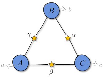
Figure 1: The triangle network features three distant parties, connected pairwise by three independent sources distributing physical systems.

Notably, it is possible to observe quantum nonlocality with parties performing a fixed measurement Fritz_2012; Branciard_2012; see also Polino2023 for a recent experiment. That is, in each round of the experiment, each party provides an output, but they receive no input. This in contrast to the standard Bell test where the use of measurement inputs is essential.

Another key aspect of the network setting is the possibility to exploit joint entangled measurements (where one or more eigenstates are non-separable) gisin2019entanglement. Similarly, as in quantum teleportation, the combination of entangled states and entangled joint measurements allows for strong correlations to be distributed across the entire network. Notably, this leads to novel forms of quantum nonlocal correlations that are genuine to the network structure Renou_2019, in the sense that they crucially rely on the use of entanglement joint measurements Supic2022; Sekatski2023. This is possible for a simple triangle network, as in Fig. 1.

While these works represent significant progress in our understanding of quantum nonlocality, they suffer from one major limitation. Namely, these proofs of genuine quantum network nonlocality are derived in an ideal noiseless setting, where the sources distribute ideal (pure) quantum states and nodes perform ideal (projective) quantum measurements. However, these proofs no longer apply when any realistic noise level is considered. This represents a major hurdle towards any practical implementation or application of these ideas, as any experiment features a certain amount of noise originating from unavoidable technical imperfections. Moreover, numerical analysis based on neural networks indicates noise-robust nonlocality krivachy_neural_2020.

One can draw a parallel with the situation of nonlocality in the mid-sixties. Indeed, John Bell’s initial proof of nonlocality applied only to the idealized case of a pure entangled state and projective local measurements Bell. A key step was then made by Clauser, Horne, Shimony and Holt who derived a noise-robust proof of quantum nonlocality via their famous CHSH Bell inequality CHSH, which enabled the first Bell experiments. This is still today the most commonly used test of nonlocality, and the basis of many applications within the device-independent approach (see e.g. review).

In this work we address the question of noise-robust proofs of quantum network nonlocality. We derive methods for this problem and discuss several examples. Our main contributions are the following. We present a general family of quantum distributions on the triangle network (without inputs) and prove their nonlocality in the ideal (noiseless) case. These distributions are based on the concept of “parity token counting” (PTC) and include as a special case the distributions of Renou et al. Renou_2019, from now on referred to as RGB4. In turn, we derive noise-robust nonlocality proofs for these quantum distributions. The key ingredient is a result of approximate rigidity for local distributions that are PTC, which allows us to deal with noise. In particular, we identify quantum distributions that remain nonlocal when up to $\sim 80\%$ dephasing noise, or $\sim 0.67$% white noise, is added at each source. Moreover, we characterize the distributions in the vicinity of a given nonlocal distribution. For a specific quantum distribution, we can show that any distribution in a $\sim 0.27$% total-variation distance ball around it is nonlocal. This can be viewed as a Bell inequality, in the sense that it guarantees that a full-measure region of the correlation set is nonlocal.

The paper is organized as follows. In Section II, we provide the general context, introduce notations, and review the concept of parity token counting (PTC) distributions. In Section III, we prove results on approximate PTC rigidity for local distributions. This allows us to bound local correlations that approximately verify the PTC condition. Additionally, we derive an analytical outer relaxation of the set of binary output correlations compatible with a triangle-local model. In Section IV, we introduce a general family of quantum nonlocal distributions. We first prove their nonlocality in the noiseless case. In turn, based on the results of Section III, we prove results on the nonlocality of these distributions in the noisy case. Finally, we conclude in Section VI and discuss future perspectives.

II Background

To start we recall some background notions and fix the notations. Consider a triangle network as in Fig. 1, where three independent sources (labeled $\alpha$, $\beta$, and $\gamma$) distribute physical systems to three distant parties (nodes $A$, $B$, and $C$). Each party thus receives two physical subsystems (from two different sources), and produces a measurement outcome, denoted by the classical variables $a$, $b$, and $c$ (of finite cardinality $d$ ). The experiment results in the joint probability distribution $P(a,b,c)$.

We aim to understand which distributions are compatible with the triangle causal network depicted in Fig. 1. The set of possible distributions depends on the underlying physical theory. We are interested here in distributions that can be realized in classical physics (where the sources produce correlated classical variables) and in quantum theory (where the sources can produce entangled states). Our focus will be on quantum distributions that cannot be realized classically, hence demonstrating network nonlocality.

First, a distribution $P_{L}(a,b,c)$ is said to be triangle-local if it admits a classical model, i.e. it can be decomposed as

$$P_{L}(a,b,c)=\mathds{E}\Big(P_{A}(a|\beta,\gamma)P_{B}(b|\gamma,\alpha)P_{C}(c|\alpha,\beta)\Big),$$ (1)

where $\mathds{E}$ is the expected value over the independently distributed classical variables $\alpha,\beta,\gamma$. Furthermore, the conditional probabilities $P_{X}(x|\xi,\xi^{\prime})$ can be considered deterministic without loss of generality, and represented by the response functions $x(\xi,\xi^{\prime})$. A distribution that does not admit a decomposition of the form (1) is termed triangle-nonlocal, or simply nonlocal in the following.

Second, we say that a distribution $P_{Q}(a,b,c)$ is triangle-quantum if it can be written as

$$\begin{split}P_{Q}(a,b,c)=\tr\Big(&\rho^{\alpha}_{B_LC_R}\otimes\rho^{\beta}_{C_LA_R}\otimes\rho^{\gamma}_{A_LB_R} \\ &\times E_{A_LA_R}^{a} \otimes E_{B_LB_R}^{b} \otimes E_{C_LC_R}^{c} \Big)\end{split}$$ (2)

where $\rho^{\xi}$ denote the quantum states distributed by the sources (density operators), and $\{E_{YY^{\prime}}^{x}\}$ denote the measurements performed at each node (POVMs). Note that one should pay attention to the order of subsystems when computing (2).

For a given output cardinality $d$ we denote the set of all triangle-local distributions $\mathcal{L}_{\triangle}^{d}$ and the set of all triangle-quantum distributions $\mathcal{Q}_{\triangle}^{d}$. In general, characterizing these sets is a challenging problem. Outer approximations can be derived Chaves2015; wolfe2019inflation; wolfe2021inflation; Aberg2020, but typically only provide loose bounds.

For $d\geq 3$, it is known that $\mathcal{L}_{\triangle}^{d}\subset\mathcal{Q}_{\triangle}^{d}$, i.e. there exists quantum distributions that are nonlocal (see Boreiri2023 and references therein). For $d=2$, this is still an open question.

Known proofs of quantum nonlocality for the triangle network are of two types. The first are distributions that can be viewed as a clever embedding of a standard Bell test (e.g. CHSH) on the triangle network without inputs. The initial construction was derived by Fritz Fritz_2012; see also Fraser; Weilenmann_2018; supic; Boreiri2023. For this class of distributions, noise-robust methods have been recently developed Chaves2021, leading to a first experiment Polino2023. Due to their connection with standard Bell tests, these distributions can be implemented without the need for any entangled measurements. Hence the nonlocality of these distributions originates solely from the use of an entangled state.

In contrast, there exist quantum distributions on the triangle network based on the judicious combination of entangled states and measurements, as first shown by Renou and colleagues Renou_2019. It was recently shown that this distribution requires in fact the use of entangled measurements Sekatski2023, hence demonstrating genuine network quantum nonlocality Supic2022. So far, these nonlocality proofs are essentially restricted to an ideal noiseless scenario see e.g. Renou_2019; renou2022network; Abiuso2022; Boreiri2023; Pozas2023). That is, they consider a setting where the shared states $\rho^{\xi}$ are pure and the local measurements $\{E_{YY^{\prime}}^{x}\}$ are projective. However, these proofs no longer apply when any realistic amount of noise is included. On the other hand, numerical analysis based on machine learning suggests that the nonlocality of these quantum distributions is in fact robust to noise krivachy_neural_2020, up to $\approx 10\%$ white noise at the sources for some instances of the RGB4 distribution. Deriving noise-robust analytical proofs is therefore an important open problem, which we address in this work.

II.1 PTC distributions and rigidity

A key class of distributions for our work is termed parity token counting (PTC). These are local distributions on the triangle network, obtained via the following model. Each source possesses a single token that it sends to either one of its connected parties with some given probability. For instance, the source $\alpha$ sends its token to Bob with probability $p_{\alpha}$ and to Charlie with probability $1-p_{\alpha}$. Then each party outputs the parity of the total number of received tokens. Therefore if we define the binary random variable $t_{\alpha}\in\{0,1\}$ as the number of tokens $\alpha$ sends to Bob, $t_{\beta}\in\{0,1\}$ as the number of tokens $\beta$ sends to Charlie, and $t_{\gamma}\in\{0,1\}$ as the number of tokens $\gamma$ sends to Alice, then for example Alice is receiving $t_{\gamma}$ from the source $\gamma$ and $t_{\beta}\oplus 1$ from the source $\beta$ and its response function woud be $a(\beta,\gamma)=t_{\gamma}\oplus t_{\beta}\oplus 1$, where $\oplus$ denotes the sum modulo two.

The distribution $P(a,b,c)$ resulting from the above PTC model has binary outputs ($d=2$). By construction, any such distribution satisfies

$$a\oplus b\oplus c=1,$$ (3)

which we refer to as the PTC condition.

Let us now explore the reverse link. Starting from a distribution that satisfies the PTC condition, what can we infer about the underlying classical model? Interestingly, PTC distributions demonstrate a form of rigidity Boreiri2023; note that this property of rigidity was initially discussed for token counting models renou2022network. Rigidity means that a PTC distribution can only be obtained via a PTC model (up to irrelevant relabellings). That is, for any local model leading to a PTC distribution, there exists for each source a token function

$$\begin{split}&T_{\xi}:\xi\to t_{\xi}\in\{0,1\}\qquad\text{such that}\\ &x(\xi,\xi^{\prime})=t_{\xi}\oplus t_{\xi^{\prime}}\oplus 1.\end{split}$$ (4)

In addition, if the probability distribution is such that $E_{a},E_{b},E_{b}\neq 0$ for $E_{x}=\text{Pr}(x=0)-\text{Pr}(x=1)$, the token functions can be chosen to fulfill

$$p_{\alpha}(t):=\text{Pr}(t_{\alpha}=t)=\frac{1}{2}\left(1+(-1)^{t}\sqrt{\left|\frac{E_{b}E_{c}}{E_{a}}\right|}\right)$$ (5)

and similar equalities of the other sources. This means that there is essentially only a unique local model over the triangle which can simulate such a distribution. In Boreiri2023 one can find a simple characterization of the local PTC set $\mathcal{L}_{\triangle|PTC}^{2}$, containing all triangle-local distributions that satisfy the PTC condition of Eq. (3). We find that this set covers about 12.5% of the volume of $\mathcal{P}_{PTC}^{2}$ – the set of binary probability distributions $P(a,b,c)$ fulfilling Eq. (3).

Remarkably the PTC rigidity, albeit formulated differently, is also true for any quantum PTC distribution Sekatski2023. In particular, this implies that in the slice of the probability set where the parity condition in Eq. (3) holds there is no separation between the quantum and local sets, i.e. $\mathcal{Q}_{\triangle|PTC}^{2}=\mathcal{L}_{\triangle|PTC}^{2}$.

III Approximate PTC rigidity for local distributions

Let us now consider a local distribution $P(a,b,c)$ for which the parity condition only holds approximately, i.e.

$$\text{Pr}(a\oplus b\oplus c=1)\geq 1-\varepsilon.$$ (6)

Intuitively, one expects the underlying local model to verify some approximate form of rigidity. This is what we now establish.

Since the response functions are deterministic, there is a set

$$\Lambda=\{\bm{\xi}|a(\beta,\gamma)\oplus b(\alpha,\gamma)\oplus c(\alpha,\beta)=1\}$$ (7)

containing all the values $\bm{\xi}=(\alpha,\beta,\gamma)$ for which the parity condition in Eq. (3) is true. By assumption we have $\text{Pr}(\bm{\xi}\in\Lambda)\geq 1-\varepsilon$.

Let us now take any value $\gamma_{*}$ for which $\text{Pr}(\bm{\xi}\in\Lambda|\gamma=\gamma_{*})\geq 1-\varepsilon$. Such a value must exist, since this probability can not be strictly lower than its average on all $\gamma$. For the chosen value of $\gamma$, we define the token function to be

$$t_{\gamma_{*}}=1.$$ (8)

Next, take $G_{*}=\{(\alpha,\beta)|(\alpha,\beta,\gamma_{*})\in\Lambda\}$ to be the set of all pairs $(\alpha,\beta)$ for which the parity condition holds when $\gamma=\gamma_{*}$. On this set we now define the token functions $t_{\alpha}$ and $t_{\beta}$ as

$$\begin{split}t_{\alpha}&=b(\alpha,\gamma_{*})\\ t_{\beta}&=a(\beta,\gamma_{*}).\end{split}$$ (9)

Let us check that for $\gamma=\gamma_{*}$ and any values $\alpha$ and $\beta$ in $G_{*}$, the PTC rigidity of Eq.(4) holds. By construction we have $t_{\beta}\oplus t_{\gamma_{*}}\oplus 1=t_{\beta}=a(\beta,\gamma_{*})$ and $t_{\alpha}\oplus t_{\gamma_{*}}\oplus 1=b(\alpha,\gamma_{*})$, while

$$t_{\beta}\oplus t_{\alpha}\oplus 1=a(\beta,\gamma_{*})\oplus b(\alpha,\gamma_{*})\oplus 1=c(\alpha,\beta)$$ (10)

follows form the parity condition at $(\alpha,\beta,\gamma_{*})\in\Lambda$. In addition, we have a lower bound on the probability that $(\alpha,\beta)$ are sampled in $G_{*}$

$$\text{Pr}\big((\alpha,\beta)\in G_{*}\big)=\text{Pr}(\bm{\xi}\in\Lambda|\gamma=\gamma_{*})\geq 1-\varepsilon.$$ (11)

Finally, consider the set

$$\Omega=\{\bm{\xi}|(\alpha,\beta)\in G_{*}\text{ and }\bm{\xi}\in\Lambda\}.$$ (12)

which has the probability

$$\begin{split}\text{Pr}(\bm{\xi}\in\Omega)&\geq 1-\text{Pr}(\bm{\xi}\notin\Lambda)-\text{Pr}((\alpha,\beta)\notin G_{*})\\ &\geq 1-2\varepsilon.\end{split}$$ (13)

For any point $(\alpha,\beta,\gamma)$ from this set we can define the prolongation of the token function $t_{\gamma}$ as

$$\begin{split}t_{\gamma}^{(\alpha,\beta)}&=1\oplus a(\beta,\gamma)\oplus a(\beta,\gamma_{*})\\ &=1\oplus b(\alpha,\gamma)\oplus b(\alpha,\gamma_{*}),\end{split}$$ (14)

where the equality of the two definitions follows from the fact that both points $(\alpha,\beta,\gamma)$ and $(\alpha,\beta,\gamma_{*})$ are inside $\Lambda$ by construction. It is also easy to see that this value $t_{\gamma}$ satisfy the PTC rigidity, i.e. $t^{(\alpha,\beta)}_{\gamma}\oplus t_{\beta}\oplus 1=a(\beta,\gamma)$ and the other equations, for the variables value $(\alpha,\beta,\gamma)$ (see Appendix A). The problem however is that the prolongations of $t_{\gamma}$ must not necessarily agree for different choices of $(\alpha,\beta)$. Hence this strategy can not be used to define the token function $t_{\gamma}$ on the whole set $\Omega$. Nevertheless, we show in the Appendix A, that there exists a subset $\Upsilon\subset\Omega$ such that

$$\text{Pr}(\bm{\xi}\in\Upsilon) \geq 1-\text{f}_{\varepsilon}\geq 1-3\varepsilon\quad\text{with}$$ (15)

$$1-\text{f}_{\varepsilon} =\begin{cases}\frac{1}{2}-\varepsilon+\frac{1-4\varepsilon}{2\sqrt{1-2\varepsilon}}&\varepsilon\leq\frac{1}{4}\\ \frac{1-2\varepsilon}{2}&\varepsilon>\frac{1}{4}\end{cases}$$ (16)

on which the token function $t_{\gamma}$ can be prolonged consistently. The key idea is to use the fact that the definitions in Eq. (14) must agree for any two points in $\Omega$ with the same $\alpha$ or $\beta$.

This demonstrates the following result holds.

Result 1. (Approximate PTC rigidity) For any triangle local model leading to a distribution $P(a,b,c)\in\mathcal{L}_{\triangle}^{2}$ that fulfills the approximate parity condition $\text{Pr}(a\oplus b\oplus c=1)\geq 1-\varepsilon$, there exists a subset $\Upsilon$ of local variable values $\bm{\xi}=(\alpha,\beta,\gamma)$ with $Pr(\bm{\xi}\in\Upsilon)\geq 1-\text{f}_{\varepsilon}$ (see Eq. 16), on which one can define the token functions $T_{\alpha},T_{\beta},T_{\gamma}$ that satisfy the PTC rigidity $a(\beta,\gamma)=T_{\beta}\oplus T_{\gamma}\oplus 1$ etc.

The set $\Upsilon$ gives rise to the following subnormalized distribution $P(a,b,c,\bm{\xi}\in\Upsilon)$ which satisfies $\sum_{a,b,c}P(a,b,c,\bm{\xi}\in\Upsilon)\geq 1-\text{f}_{\varepsilon}$. For simplicity let us assume that this bound is tight (otherwise one can repeat the following discussion with a second parameter $\text{f}^{\prime}\leq\text{f}_{\varepsilon}$ and reach the same conclusions), it follows that

$$P(a,b,c,\bm{\xi}\in\Upsilon)+\text{f}_{\varepsilon}P^{\prime}(a,b,c)=P(a,b,c),$$ (17)

where $P^{\prime}(a,b,c)$ is some (non necessarily local) distribution.

Now, let us prolong the token functions $T_{\xi}$ to all the values of the local variables that do not appear in $\Upsilon$, this can be done by e.g. assigning $t_{\xi}=0$ to all such values. With the token functions defined everywhere, we can now define a new probability distribution

$$\widetilde{P}(a,b,c)=\mathds{E}\Big(P_{\scriptscriptstyle ptc}(a|t_{\beta},t_{\gamma})P_{\scriptscriptstyle ptc}(b|t_{\alpha},t_{\gamma})P_{\scriptscriptstyle ptc}(c|t_{\alpha},t_{\beta})\Big)$$ (18)

where the outputs are obtained with the PTC response functions

$$P_{\scriptscriptstyle ptc}(x|t_{\xi},t_{\xi^{\prime}})=\begin{cases}1&x=t_{\xi}\oplus t_{\xi^{\prime}}\oplus 1\\ 0&x\neq t_{\xi}\oplus t_{\xi^{\prime}}\oplus 1\end{cases}.$$ (19)

By construction, this distribution is triangle local and PTC. Furthermore, we know that $P(a,b,c)$ and $\widetilde{P}(a,b,c)$ agree on the subset $\bm{\xi}\in\Upsilon$, hence the identity

$$P(a,b,c,\bm{\xi}\in\Upsilon)+\text{f}_{\varepsilon}\widetilde{P}^{\prime}(a,b,c)=\widetilde{P}(a,b,c)$$ (20)

holds for some PTC (non-necessarily local) distributions $\widetilde{P}^{\prime}$. Combining Eqs. (17,20) we conclude that the observed local distribution must satisfy $P(a,b,c)=\widetilde{P}(a,b,c)-\text{f}_{\varepsilon}\widetilde{P}^{\prime}(a,b,c)+\text{f}_{\varepsilon}P^{\prime}(a,b,c)$, which can be nicely expressed in terms of total variation distance

$$\delta(P,\widetilde{P})=\frac{1}{2}\sum_{a,b,c}|P(a,b,c)-\widetilde{P}(a,b,c)|\leq\text{f}_{\varepsilon}.$$ (21)

We have thus shown that any local distribution $P(a,b,c)$ satisfying the approximate parity condition of Eq. (6), must be close to the local PTC set

$$\delta(P,\mathcal{L}^{2}_{\triangle|PTC})=\min_{\widetilde{P}\in\mathcal{L}_{\triangle|PTC}^{2}}\delta(P,\widetilde{P})\leq\text{f}_{\varepsilon}$$ (22)

In turn, the approximate parity condition is equivalent to a bound on the total variation distance between $P$ and the PTC slice of the probability set $\delta(P,\mathcal{P}_{PTC}^{2})=\min_{Q\in\mathcal{P}_{PTC}^{2}}\delta(P,Q)\leq\varepsilon.$ Therefore, we have shown the following result.

Result 2.(Relaxation of the local set $\mathcal{L}_{\triangle}^{2}$) Any triangle local distribution $P(a,b,c)\in\mathcal{L}_{\triangle}^{2}$ that is close to the PTC slice of the probability set $\delta(P,\mathcal{P}_{PTC}^{2})\leq\varepsilon$ is also close to the local PTC set $\delta(P,\mathcal{L}^{2}_{\triangle|PTC})\leq\text{f}_{\varepsilon}$ (see Eq. 16).

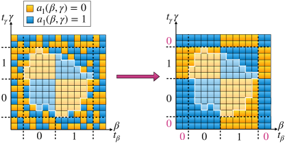
Figure 2: A graphical representation of the construction used in the proof of approximate PTC rigidity. The coordinates along the axes represent different values of the local variables $\beta$ and $\gamma$, here discredited to 15 possible values each. The color of each square gives the value of Alice’s outcome $a(\beta,\gamma)=0$ (yellow) and $a(\beta,\gamma)=1$ (blue). On the left, the lighter region depicts the set $\Upsilon$ on which the binary token functions $t_{\beta}$ and $t_{\gamma}$ are defined (given below the axes) and satisfy $a(\beta,\gamma)=t_{\beta}\oplus t_{\gamma}\oplus 1$. On the right, the token functions are prolonged on the whole set of local variables by setting them to 0 outside of $\Upsilon$. The values obtained by applying the PTC response function $a(\beta,\gamma)=t_{\beta}\oplus t_{\gamma}\oplus 1$ (right) are not guaranteed to match the observed values $a(\beta,\gamma)$ (left) outside of $\Upsilon$.

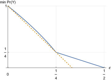
In words, the approximate rigidity allows us to define a cone of distributions $\widehat{\mathcal{L}}^{2}_{\triangle}$ that are accessible when going away from the PTC slice. Loosely speaking – if we only move a distance $\varepsilon$ from $\mathcal{L}_{\triangle|PTC}^{2}$ perpendicular to the PTC slice we can not move more than a distance $\varepsilon$ inside the slice. Any distribution outside of the cone is guaranteed to be nonlocal, i.e. we have established an outer approximation of the local set $\mathcal{L}_{\triangle}^{2}\subset\widehat{\mathcal{L}}^{2}_{\triangle}$. It is an open question whether all quantum distributions are also contained in this cone.

To illustrate Result 2 we discuss the nonlocality of the noisy W distributions (see Appendix B).

IV Noise-robust nonlocality in $\mathcal{Q}^{4}_{\triangle}$

We now consider a particular family of four-outcome quantum distributions on the triangle. Those are obtained from the following quantum models. Each source distributes a two-qubit state

$$\ket{\psi}=\lambda_{0}\ket{01}+\lambda_{1}\ket{10},$$ (23)

with real and positive $\lambda_{0}^{2}+\lambda_{1}^{2}=1$, to the neighbouring parties. While each party performs the same projective measurement $\{\Pi_{x_{1},x_{2}}=\outerproduct{\phi_{x_1,x_2}}{\phi_{x_1,x_2}}\}$ on the two qubits it receives from neighboring sources, with the POVM elements given by projectors on the states

$$\begin{split}\ket{\phi_{1,0}}&=u\ket{0,1}+v\ket{1,0}\\ \ket{\phi_{1,1}}&=v\ket{0,1}-u\ket{1,0}\\ \ket{\phi_{0,0}}&=w\ket{0,0}+z\ket{1,1}\\ \ket{\phi_{0,1}}&=z\ket{0,0}-w\ket{1,1}\end{split}$$ (24)

with real positive $u,v,w,z$ satisfying $u^{2}+v^{2}=w^{2}+z^{2}=1$. The resulting family of quantum distribution is termed “tilted Bell state measurements” (TBSM) distribution, since the local measurements can be viewed as tilted Bell state measurements.

$$P(1,i,1,j,1,k) =(\lambda_{0}^{3}u_{i}u_{j}u_{k}+\lambda_{1}^{3}v_{i}v_{j}v_{k})^{2}$$ (25)

$$P(1,i,0,j,0,k) =(\lambda_{0}\lambda_{1}^{2}u_{i}w_{j}z_{k}+\lambda_{1}\lambda_{0}^{2}v_{i}w_{k}z_{j})^{2}\,\circlearrowleft$$ (26)

where $u_{0}=u,\,v_{0}=v\,,w_{0}=w\,,z_{0}=z,\,u_{1}=v,\,v_{1}=-u,\,w_{1}=z$ and $z_{1}=-w$

By setting $w=1-z=0$ one recovers the RGB4 family of distributions Renou_2019, while merging the outcomes $(0,0)$ and $(0,1)$ leads to the three-output family of quantum distributions introduced in Boreiri2023.

As a warm-up, we now present a proof of nonlocality of the distributions in Eq. (25) for a subset of parameter values $(\lambda_{0},u,m)$. It has the advantage of streamlining the proof techniques used in Renou_2019 and subsequently Boreiri2023, while relying on the same basic idea, This will be helpful when we move to the noisy case.

IV.1 Nonlocality of the noiseless TBSM distributions

The nonlocality proof proceeds by contradiction, so let us assume that the distribution is local. It is easy to see that when the second output is discarded, the resulting binary distributions

$$P(a_{1},b_{1},c_{1})=\sum_{a_{2},b_{2},c_{2}}P(a_{1},a_{2},b_{1},b_{2},c_{1},c_{2})$$ (27)

satisfy the parity condition $a_{1}\oplus b_{1}\oplus c_{1}=1$. By rigidity, it follows that for any underlying local model there exist the binary token functions $T_{\xi}$ that explain the distribution

$$P(\bm{x}_{1})=\mathds{E}\Big(P_{\scriptscriptstyle PTC}(\bm{x}_{1}|\bm{t})\Big),$$ (28)

where we introduced the compact notation $\bm{x}_{i}=(a_{i},b_{i},c_{i})$, $\bm{t}=(t_{\alpha},t_{\beta},t_{\gamma})$ and

$$P_{\scriptscriptstyle PTC}(\bm{x}_{1}|\bm{t})=P_{\scriptscriptstyle ptc}(a_{1}|t_{\beta},t_{\gamma})P_{\scriptscriptstyle ptc}(b_{1}|t_{\alpha},t_{\gamma})P_{\scriptscriptstyle ptc}(c_{1}|t_{\alpha},t_{\beta}),$$

with the response functions of Eq. (19). Furthermore, if $E_{a_{1}},E_{b_{1}},E_{c_{1}}\neq 0$ the token distribution $p(\bm{t})=p_{\alpha}(t_{\alpha})p_{\beta}(t_{\beta})p_{\gamma}(t_{\gamma})$ is known exactly via Eq. (5).

This conclusion is of course independent of whether we discard the outcomes $\bm{x}_{2}$ or not. Hence, for any local model resulting in the TBSM distribution, we can define the random variable $\bm{t}$, indicating the behavior of the tokens, using the Chain rule we have $P(\bm{x}_{1},\bm{x}_{2})=\sum_{\bm{t}}p(\bm{t})P(\bm{x}_{2}|\bm{t})P(\bm{x}_{1}|\bm{t},\bm{x}_{2})$. From the rigidity, we can infer that $\bm{x}_{1}$ is solely a function of $\bm{t}$, leading to

$$\begin{split}P(\bm{x}_{1},\bm{x}_{2})=\sum_{\bm{t}}p(\bm{t})P_{\scriptscriptstyle PTC}(\bm{x}_{1}|\bm{t})P(\bm{x}_{2}|\bm{t}).\end{split}$$ (29)

Here, all the distributions $P(\bm{x}_{2}|\bm{t})\in\mathcal{L}_{\triangle}^{2}$ must be triangle local. Furthermore, these distributions are not independent, since the output of a party (e.g. $a_{2}$) can not be influenced by the source that is not connected to it (that is by $\alpha$ and the token value $t_{\alpha}$). This observation implies the following constraints on the marginal distributions $P(a_{2}|\bm{t})=\sum_{b_{2},c_{2}}P(\bm{x}_{2}|\bm{t})$

$$P(a_{2}|t_{\alpha}=0,t_{\beta},t_{\gamma})=P(a_{2}|t_{\alpha}=1,t_{\beta},t_{\gamma})\quad\circlearrowleft$$ (30)

and similar constraints for all permutations of parties, as indicated by the symbol $\circlearrowleft$. The above discussion can be summarized as follows.

Result 3. (Nonlocality of TBSM distributions) For any triangle local distribution $P(\bm{x}_{1},\bm{x}_{2})\in\mathcal{L}_{\triangle}^{4}$ satisfying $a_{1}\oplus b_{1}\oplus c_{1}=1$ , there exist eight probability distributions $P(\bm{x}_{2}|\bm{t})$ such that

$$\begin{split}&(3.i)\,P(\bm{x}_{1},\bm{x}_{2})=\sum_{\bm{t}}p(\bm{t})P_{\scriptscriptstyle PTC}(\bm{x}_{1}|\bm{t})P(\bm{x}_{2}|\bm{t})\\ &(3.ii)\,P(a_{2}|t_{\alpha}=0,t_{\beta},t_{\gamma})=P(a_{2}|t_{\alpha}=1,t_{\beta},t_{\gamma})\quad\circlearrowleft\\ &(3.iii)\,P(\bm{x}_{2}|\bm{t})\in\mathcal{L}_{\triangle}^{2}\qquad\forall\bm{t}\end{split}$$ (31)

where $P_{\scriptscriptstyle PTC}$ is the parity token counting response function and the token distribution $p(\bm{t})=p_{\alpha}(t_{\alpha})p_{\beta}(t_{\beta})p_{\gamma}(t_{\gamma})$ is uniquely determined from $P(\bm{x}_{1})$ via Eq. (5) (except degenerate cases were it is not unique).

If we were able to show that these conditions can not be satisfied together, we could conclude that the distribution $P(\bm{x}_{1},\bm{x}_{2})$ is nonlocal. Yet, the locality condition $(3.iii)$ here is very challenging to formalize since we do not have a good characterization of the local set $\mathcal{L}_{\triangle}^{2}$. A simple solution is to relax it and keep the other two conditions. This relaxation gives rise to a simple linear program (LP) that must be feasible for any triangle local $P(\bm{x}_{1},\bm{x}_{2})$ with $a_{1}\oplus b_{1}\oplus c_{1}=1$, that we give in appendix C.

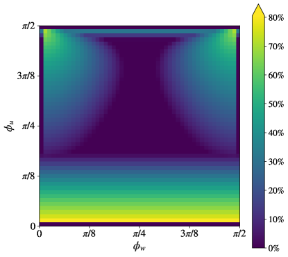
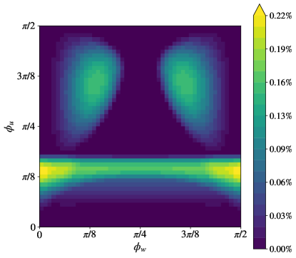
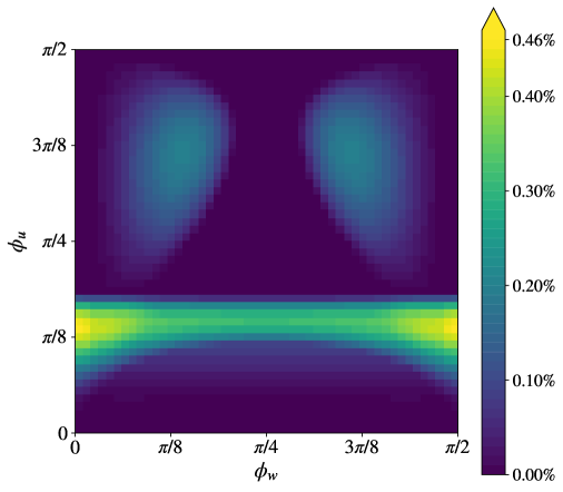
Figure 3: Nonlocality of noiseless TBSM distributions. Nonlocal region depicted in yellow. Here distributions are parametrized via angles: $u=\cos(\phi_u)$, $w=\cos(\phi_w)$. Parameter: $\lambda_{0}^{2}=0.22$.

In Fig. 3, we present the results of the LP for $\lambda_{0}^{2}=0.22$. One notes that Result 3 can be used to prove the nonlocality of the noisy distribution, if the noise does not perturb the parity of the $\bm{x}_{1}$ outcomes. For example, the local dephasing noise given by the channel $\mathcal{E}_{d}:\outerproduct{\psi}{\psi}\mapsto\varrho$ with

$$\varrho=(1-d)\outerproduct{\psi}{\psi}+d\left(\lambda_{0}^{2}\outerproduct{01}{01}+\lambda_{1}^{2}\outerproduct{10}{10}\right)$$ (32)

is of this type. In the appendix C we give the LP which finds the minimal amount of dephasing noise such that the distribution becomes triangle local. Its results are presented in Fig. 4 for $\lambda_{0}^{2}=0.22$.

Figure 4: Dephasing Noise Robustness. The amount of local dephasing noise $d$ in Eq. (32) below which the TBSM distribution is guaranteed to be nonlocal. Parameters: $u=\cos(\phi_u)$, $w=\cos(\phi_w)$ and $\lambda_{0}^{2}=0.22$.

Nevertheless, this still only applies to a slice of the quantum set $\mathcal{Q}_{\triangle}^{4}$. In the next section, we derive an approach that singles out the nonlocality of a full-measure subset of triangle quantum distributions. Interestingly, we observe that the largest robustness to white noise, as well as for total-variation distance, is obtained for the same parameters $\lambda_{0}^{2}=0.22,\phi_{u}=0.42$.

IV.2 Nonlocality of the noisy TBSM distributions

Our main idea now is pretty simple – adjust the LP-based nonlocality proof of the previous section to the setting of approximate PTC rigidity discussed in Section III.

Indeed, let us consider any triangle local distribution

$$P(\bm{x}_{1},\bm{x}_{2})=\mathds{E}\big(P_{A}(a_{1},a_{2}|\beta,\gamma)P_{B}(b_{1},b_{2}|\alpha,\gamma)P_{C}(\dots)\big)$$

such that $\text{Pr}(a_{1}\oplus b_{1}\oplus c_{1}=1)\geq 1-\varepsilon$. By approximate PTC rigidity, we know that there exists a local PTC distribution $\widetilde{P}(\bm{x}_{1})$ such that $\delta(P(\bm{x}_{1}),\widetilde{P}(\bm{x}_{1}))\leq\text{f}_{\varepsilon}.$ This distribution was constructed by applying the token functions $T_{\xi}$ to the sources, and replacing the detectors with the parity token counting response functions (See Fig. 2). This construction does not require us to discard the outcomes $\bm{x}_{2}$, and we can define a full distribution

$$\widetilde{P}(\bm{x}_{1},\bm{x}_{2})=\mathds{E}\big(P_{\scriptscriptstyle PTC}(\bm{x}_{1}|\bm{t})P_{A}(a_{2}|\beta,\gamma)P_{B}(b_{2}|\alpha,\gamma)\dots).$$ (33)

The distribution $\widetilde{P}$ is triangle local, by construction it agrees with the initial distribution on outcomes $\bm{x}_{2}$ ($\widetilde{P}(\bm{x}_{2})=P(\bm{x}_{2})$), and is PTC local for the outcomes $\bm{x}_{1}$. Furthermore, we know that the two distributions match $P(\bm{x}_{1},\bm{x}_{2},\bm{\xi}\in\Upsilon)=\widetilde{P}(\bm{x}_{1},\bm{x}_{2},\bm{\xi}\in\Upsilon)$ on the subset $\Upsilon$ of local variable values with $\text{Pr}(\bm{\xi}\in\Upsilon)\geq 1-\text{f}_{\varepsilon}$, which is equivalent to a bound on their total variation distance

$$\delta(P(\bm{x}_{1},\bm{x}_{2}),\widetilde{P}(\bm{x}_{1},\bm{x}_{2}))\leq\text{f}_{\varepsilon}.$$ (34)

We have thus reached the following conclusion.

Result 4. (Nonlocality of noisy TBSM distribution) For any triangle local distribution $P(\bm{x}_{1},\bm{x}_{2})\in\mathcal{L}_{\triangle}^{4}$ satisfying $\text{Pr}(a_{1}\oplus b_{1}\oplus c_{1}=1)\geq 1-\varepsilon$, there exists a triangle local distribution $\widetilde{P}(\bm{x}_{1},\bm{x}_{2})$ such that

$$\begin{split}&(4.i)\,\widetilde{P}(\bm{x}_{1},\bm{x}_{2})=0\quad\text{for}\quad a_{1}\oplus b_{1}\oplus c_{1}\neq 1\\ &(4.ii)\,\delta(P(\bm{x}_{1},\bm{x}_{2}),\widetilde{P}(\bm{x}_{1},\bm{x}_{2}))\leq\text{f}_{\varepsilon}.\\ &(4.iii)\,\sum_{\bm{x}_{1}}\widetilde{P}(\bm{x}_{1},\bm{x}_{2})=\sum_{\bm{x}_{1}}P(\bm{x}_{1},\bm{x}_{2})\end{split}$$ (35)

In turn, the distribution $\widetilde{P}$ satisfies the premises of the Result 3. We could thus verify the nonlocality of $P$ by showing that no distribution $\widetilde{P}$ compatible with both Result 3 and 4 exists. A complication here is that the relation (5) between the distribution $\widetilde{P}(\bm{x}_{1})$ and the underlying token distribution $p(\bm{t})$ is non-linear. It is thus easier to introduce the token distributions $p_{\alpha},p_{\beta},p_{\gamma}$ as additional variables rather than computing them from $\widetilde{P}$. That way we can combine results 3 and 4 into the following corollary.

Corollary of 4. For any triangle local distribution $P(\bm{x}_{1},\bm{x}_{2})\in\mathcal{L}_{\triangle}^{4}$ satisfying $\text{Pr}(a_{1}\oplus b_{1}\oplus c_{1}=1)\geq 1-\varepsilon$, there exist probability distributions $P(\bm{x}_{2}|\bm{t})$, $p_{\xi}(t_{\xi})$ and $\widetilde{P}(\bm{x}_{1},\bm{x}_{2})$ such that $(4.ii),(4.iii),(3.ii),(3.iii)$ and

$$(*)\,\widetilde{P}(\bm{x}_{1},\bm{x}_{2})=\sum_{\bm{t}}p(\bm{t})P_{\scriptscriptstyle PTC}(\bm{x}_{1}|\bm{t})P(\bm{x}_{2}|\bm{t})$$ (36)

for $p(\bm{t})=p_{\alpha}(t_{\alpha})p_{\beta}(t_{\beta})p_{\gamma}(t_{\gamma})$.

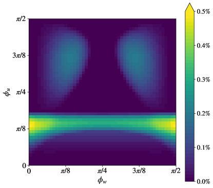
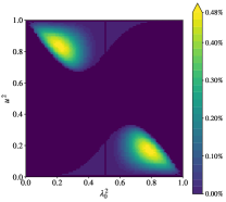
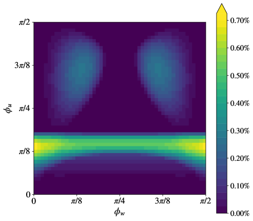
Figure 5: White Noise Robustness. Maximal amount of white noise below which we can prove the nonlocality of TBSM distributions. The largest amount of noise that can be tolerated is here $\omega=0.5\%$; note that this value can be improved slightly to $\omega=0.544\%$ (see Appendix. D.1). Parameters: $u=\cos(\phi_u)$, $w=\cos(\phi_w)$ and $\lambda_{0}^{2}=0.22$.

As in the ideal case to verify this feasibility problem we start by forgetting the condition $(3.iii)$ requiring the distributions $P(\bm{x}_{2}|\bm{t})$ to be local. Note also that the condition $(4.ii)$ on the total variation distance $\delta(P,\widetilde{P})\leq\text{f}_{\varepsilon}$ is equivalent to the existence of two probability distributions $P^{\prime}(\bm{x}_{1},\bm{x}_{2})$ and $\widetilde{P}^{\prime}(\bm{x}_{1},\bm{x}_{2})$ fulfilling $P+\text{f}_{\varepsilon}P^{\prime}=\widetilde{P}+\text{f}_{\varepsilon}\widetilde{P}$. By introducing these probabilities as variables we can rewire the conditions $(4.iii)$ and $(*)$ as

$$(4.iii^{\prime})\, \sum_{\bm{x}_{1}}\widetilde{P}^{\prime}(\bm{x}_{1},\bm{x}_{2})=\sum_{\bm{x}_{1}}P^{\prime}(\bm{x}_{1},\bm{x}_{2})$$ (37)

$$(*^{\prime})\, P(\bm{x}_{1},\bm{x}_{2})+\text{f}_{\varepsilon}\big(P^{\prime}(\bm{x}_{1},\bm{x}_{2})-\widetilde{P}^{\prime}(\bm{x}_{1},\bm{x}_{2})\big)$$

$$=\sum_{\bm{t}}p(\bm{t})P_{\scriptscriptstyle PTC}(\bm{x}_{1}|\bm{t})P(\bm{x}_{2}|\bm{t})$$ (38)

and get rid of $(4.ii)$ and the variable $\widetilde{P}(\bm{x}_{1},\bm{x}_{2})$. Finally, it is also possible to directly bound the values of the token probabilities $p_{\xi}(t_{\xi})$ from $(4.ii)$. One easily sees that the total variation distance implies $|\widetilde{E}_{x_{1}}-E_{x_{1}}|\leq 2\text{f}_{\varepsilon}$. In fact, a slightly better bound can be obtained by using the fact that $\widetilde{P}$ is in the PTC slice

$$|\widetilde{E}_{x_{1}}-E_{x_{1}}^{\Lambda}|\leq 2\text{f}_{\varepsilon}-\varepsilon,$$ (39)

where $E_{x_{1}}^{\Lambda}=\text{Pr}(x_{1}=0,a_{1}\oplus b_{1}\oplus c_{1}=1)-\text{Pr}(x_{1}=1,a_{1}\oplus b_{1}\oplus c_{1}=1)$. Hence, if all the correlators for the observed distribution satisfy $|E^{\Lambda}_{x_{1}}|>(2\text{f}_{\varepsilon}-\varepsilon)$ one can use Eq. (5) to obtain

$$\begin{split}\frac{1}{2}&\left(1+\sqrt{\frac{(|E_{b_{1}}^{\Lambda}|-(2\text{f}_{\varepsilon}-\varepsilon))(|E_{c_{1}}^{\Lambda}|-(2\text{f}_{\varepsilon}-\varepsilon))}{|E_{a_{1}}^{\Lambda}|+(2\text{f}_{\varepsilon}-\varepsilon)}}\right)\leq p_{\alpha}(0)\\ &\leq\frac{1}{2}\left(1+\sqrt{\frac{(|E_{b_{1}}^{\Lambda}|+(2\text{f}_{\varepsilon}-\varepsilon))(|E_{c_{1}}^{\Lambda}|+(2\text{f}_{\varepsilon}-\varepsilon))}{|E_{a_{1}}^{\Lambda}|-(2\text{f}_{\varepsilon}-\varepsilon)}}\right)\quad\circlearrowleft.\end{split}$$ (40)

In the Appendix D we show how using this bound the feasibility problem in Eq. (36) can be relaxed to an LP, or a tighter collection of LPs for a grid of values $p_{\xi}(0)$. To illustrate this approach we now consider the family of noisy TBSM distributions, where local white noise is added to the pure state in Eq. (23) leading to the density operator

$$\rho=(1-\omega)\outerproduct{\psi}{\psi}+\omega\frac{\mathds{1}}{2}\otimes\frac{\mathds{1}}{2}.$$ (41)

The resulting distribution satisfies $\text{Pr}(a_{1}\oplus b_{1}\oplus c_{1}=1)=\frac{1}{2}\left(1+(1-\omega)^{3}\right)$. In Fig. 5 we plot the maximal amount of white noise $\omega$ for which we can prove the nonlocality of the distribution for $\lambda_{0}^{2}=0.22$ and different measurement parameters. The maximal value that we find is about $\omega=0.67\%$ at $\phi_{u}=0.42$.

In Appendix E we also discuss the nonlocality of the distributions for white noise at the measurements, measurements with a no-click probability, as well as photon-number-resolving detectors with limited efficiency in the case of the single-photon entanglement implementation Abiuso2022.

Figure 6: Total Variation. The size of the total variation distance ball $\mathcal{B}_{\varepsilon}(\bar{P})$ in Eq. (42) around the ideal TBSM distributions, for which we prove nonlocality. The maximal value we find is $\varepsilon=0.22\%$, which can be improved to $\varepsilon=0.24\%$ (see Appendix. D.1). Parameters: $u=\cos(\phi_u)$, $w=\cos(\phi_w)$ and $\lambda_{0}^{2}=0.22$.

IV.3 Nonlocality of regions of the quantum set.

So far we argued how the nonlocality of a given distribution $P(\bm{x}_{1},\bm{x}_{2})$ can be demonstrated. However, to better understand the separation between the quantum and the local sets it is more insightful to derive expressions that single out whole regions of the quantum sets that are guaranteed to be nonlocal, similarly to the usual Bell tests. In the case of nonlocality without inputs, considered here, such expression must be nonlinear. We now derive such ”Bell tests” in terms of total variation distance balls around a target quantum distribution.

Given a target quantum distribution $\bar{P}(\bm{x}_{1},\bm{x}_{2})\in\mathcal{Q}_{\triangle}^{4}$ define the total variation distance ball as the following subset of the correlation set

$$\mathcal{B}_{\varepsilon}(\bar{P})=\{P\in\mathcal{P}_{\triangle}^{4}|\delta(P,\bar{P})\leq\varepsilon\}.$$ (42)

We will now show that for well-chosen target distributions $\bar{P}$ and small enough $\varepsilon$ the whole set $\mathcal{B}_{\varepsilon}(\bar{P})$ is nonlocal.

Concretely, consider $\bar{P}$ such that $a_{1}\oplus b_{1}\oplus c_{1}=1$. Any distribution $P\in\mathcal{B}_{\varepsilon}(\bar{P})$ must satisfy

$$\text{Pr}(a_{1}\oplus b_{1}\oplus c_{1}=1)\geq 1-\varepsilon.$$ (43)

In addition, if the ball contains some triangle local distribution $P$ by Result 4 there must exist a local PTC distribution $\widetilde{P}$ with $\delta(\widetilde{P}(\bm{x}_{1},\bm{x}_{2}),P(\bm{x}_{1},\bm{x}_{2}))\leq\text{f}_{\varepsilon}$ by (4.ii) and $\delta(\widetilde{P}(\bm{x}_{2}),P(\bm{x}_{2}))=0$ by (4.iii). By the triangle inequality, $\widetilde{P}$ must also satisfy

$$\delta(\widetilde{P}(\bm{x}_{1},\bm{x}_{2}),\bar{P}(\bm{x}_{1},\bm{x}_{2})) \leq\delta(\widetilde{P},P)+\delta(P,\bar{P})\leq\text{f}_{\varepsilon}+\varepsilon$$

$$\delta(\widetilde{P}(\bm{x}_{2}),\bar{P}(\bm{x}_{2})) \leq 0+\delta(P,\bar{P})\leq\varepsilon,$$

leading to the following conclusion.

Result 5. (Nonlocality of a ball $B_{\varepsilon}(\bar{P})$) If the ball $B_{\varepsilon}(\bar{P})\subset\mathcal{P}_{\triangle}^{4}$ contains triangle local distributions, there exists a triangle local distribution $\widetilde{P}(\bm{x}_{1},\bm{x}_{2})$ such that

$$\begin{split}&(5.i)\,\widetilde{P}(\bm{x}_{1},\bm{x}_{2})=0\quad\text{for}\quad a_{1}\oplus b_{1}\oplus c_{1}\neq 1\\ &(5.ii)\,\delta(\bar{P}(\bm{x}_{1},\bm{x}_{2}),\widetilde{P}(\bm{x}_{1},\bm{x}_{2}))\leq\text{f}_{\varepsilon}+\varepsilon.\\ &(5.iii)\,\delta(\bar{P}(\bm{x}_{2}),\widetilde{P}(\bm{x}_{2}))\leq\varepsilon.\end{split}$$ (44)

Naturally, this can be combined with the Result 3 in order to show that no local distribution $\widetilde{P}$ fulfilling $(5.i)-(5.iii)$ can exist. The argumentation is fairly similar to the corollary of the result 4, and it is pointless to repeat in the main text. In the Appendix F we present an LP relaxation of this feasibility problem. In Fig. 6 we plot the size of the ball $\varepsilon$ around the TBSM distributions with $\lambda_{0}^{2}=0.22$ which we prove to be nonlocal. The largest value we find is $\varepsilon=0.27\%$ and it is achieved for an RGB4 distribution ($w=0$).

V Discussion

We have derived noise-robust proofs of quantum nonlocality in the triangle network without inputs. Our key ingredient is a result of approximate rigidity for parity token (PTC) local distributions. This allowed us to obtain bounds on the admissible noise for a general family of quantum distributions that we introduced, generalizing the RGB4 distributions Renou_2019. We characterized noise-robustness in terms of limited visibility for the source states, considering dephasing and white noise. Alternatively, we can also characterize distributions in the vicinity of a target distribution, via a bound on the total-variation distance.

Our work opens different perspectives. First, it would be interesting to see if our methods can be applied to larger networks and distributions satisfying PTC. This may lead to proofs of network nonlocality that are more robust to noise compared to the present results.

Another direction is to see how to strengthen the noise robustness for the nonlocality proof in our Result 4. A promising option is to revisit Result 3, and strengthen the last condition (3.iii). We used the standard implementation of the inflation technique, but stronger versions could be obtained by exploiting nonlinear constraints. While we could prove robustness to white noise up to $0.67\%$, there is still potential for significant improvements; indeed numerical methods krivachy_neural_2020 suggests robustness of up to $\sim 10\%$. Any progress in this direction would be relevant, in particular from the perspective of experimental demonstrations. Concerning dephasing noise, we demonstrated strong robustness, up to $\sim 80\%$. We conjecture that there exist quantum distributions that can tolerate an amount of dephasing noise arbitrarily close to one.

It would also be interesting to see if the property of approximate PTC rigidity can be extended from local models to quantum ones. If not, this could indicate the existence of quantum nonlocal correlations in the triangle network with binary outputs (and no inputs).

Code availability.— Our implementation of the method for the triangle network can be found at https://github.com/SadraBoreiri/Robust-Nework-Nonlocality

Acknowledgements.— We thank Wolfgang Dür for discussions at the early stage of this project, and Victor Gitton for useful comments on the first version of the paper. We acknowledge financial support from the Swiss National Science Foundation (project 2000021 and NCCR SwissMAP) and by the Swiss Secretariat for Education, Research and Innovation (SERI) under contract number UeM019-3.

Appendix A Approximate PTC rigidity

Consider variables $\alpha$, $\beta$,$\gamma$ sampled from the sets $A,B,C$ with some probability distributions/densities, and deterministic response function $a(\beta,\gamma),b(\alpha,\gamma),c(\alpha,\beta)\in\{0,1\}$. Let there be a subset $\Lambda\subset A\times B\times C$ such that

$$a(\beta,\gamma)\oplus b(\alpha,\gamma)\oplus c(\alpha,\beta)=1\quad\forall\,\bm{\xi}=(\alpha,\beta,\gamma)\in\Lambda$$ (45)

$$\text{Pr}(\Lambda)=\text{Pr}(\bm{\xi}\in\Lambda)=1-\varepsilon.$$ (46)

For each value $\gamma$ define the set

$$G_{\gamma}=\{(\alpha,\beta)|(\alpha,\beta,\gamma)\in\Lambda\}\subset A\times B$$ (47)

as the slice of $\Lambda$ for a fixed $\gamma$. The probabilities of these sets $\text{Pr}(G_{\gamma})=\text{Pr}((\alpha,\beta)\in G_{\gamma})$ satisfy the following equality

$$\mathds{E}(\text{Pr}(G_{\gamma}))=\text{Pr}((\alpha,\beta,\gamma)\in\Lambda)=\text{Pr}(\Lambda)=1-\varepsilon,$$ (48)

where the expected value on the left-hand side is taken with respect to $\gamma$. Let us now identify the value $\gamma_{*}$ for which $\text{Pr}(G_{\gamma})$ is maximal, i.e.

$$\gamma_{*}=\text{argmax}_{\gamma}\text{Pr}(G_{\gamma})$$ (49)

$$1-\varepsilon_{*}=\max_{\gamma}\text{Pr}(G_{\gamma}).$$ (50)

By construction we have $\text{Pr}(G_{\gamma})\leq 1-\varepsilon_{*}$ for all $\gamma$, and $\varepsilon_{*}\leq\varepsilon$ since the maximum is larger than the average. To shorten the notation we dub $G_{*}=G_{\gamma_{*}}$.

On the set $G_{*}$ define the token functions

$$T_{\alpha}:=b(\alpha,\gamma_{*})\qquad T_{\beta}:=a(\beta,\gamma_{*})$$ (51)

as well as the value $T_{\gamma_{*}}=1$. It is easy to see that on the set $G_{*}\times\{\gamma_{*}\}\subset\Lambda$ these function satisfy the PTC rigidity conditions given by

$$T_{\beta}\oplus T_{\gamma_{*}}\oplus 1 =a(\beta,\gamma_{*})$$ (52)

$$T_{\alpha}\oplus T_{\gamma_{*}}\oplus 1 =b(\alpha,\gamma_{*})$$ (53)

$$T_{\beta}\oplus T_{\alpha}\oplus 1 =a(\beta,\gamma_{*})\oplus b(\alpha,\gamma_{*})\oplus 1=c(\alpha,\beta),$$ (54)

where we used $a(\beta,\gamma_{*})\oplus b(\alpha,\gamma_{*})\oplus c(\alpha,\beta)=1$ in the last line.

Now consider a different value $\gamma$ and the corresponding set $G_{\gamma}$. Furthermore, define the set

$$S_{\gamma}=G_{\gamma}\cap G_{*}=\{(\alpha,\beta)|(\alpha,\beta)\in G_{*},(\alpha,\beta,\gamma)\in\Lambda\}.$$ (55)

It is a subset of both $G_{*}$ and $G_{\gamma}$, hence each $(\alpha,\beta)\in S_{\gamma}$, both $(\alpha,\beta,\gamma)$ and $(\alpha,\beta,\gamma_{*})$ are inside $\Lambda$. We denote

$$1-\delta_{\gamma}=\text{Pr}\big(S_{\gamma}),$$ (56)

which must satisfy $\delta_{\gamma}\geq\varepsilon_{*}$ because $S_{\gamma}\subset G_{*}$.

Remaining in the slice $\gamma$, can define the following binary functions

$$t_{\alpha}^{z} :=b(\alpha,\gamma)\oplus z\oplus 1$$ (57)

$$t^{z}_{\beta} :=a(\beta,\gamma)\oplus z\oplus 1$$ (58)

$$t_{\gamma}^{z} :=z.$$ (59)

For both choices $z=0$ and $z=1$, there functions satisfy the PTC conditions on the set $S_{\gamma}\times\{\gamma\}$

$$t^{z}_{\alpha}\oplus t_{\gamma}^{z}\oplus 1 =b(\alpha,\gamma)\oplus z\oplus 1\oplus z\oplus 1=b(\alpha,\gamma)$$ (60)

$$t^{z}_{\beta}\oplus t_{\gamma}^{z}\oplus 1 =a(\beta,\gamma)\oplus z\oplus 1\oplus z\oplus 1=a(\beta,\gamma)$$ (61)

$$t_{\alpha}^{\gamma}\oplus t_{\beta}^{\gamma}\oplus 1 =b(\alpha,\gamma)\oplus a(\beta,\gamma)\oplus 1=c(\alpha,\beta),$$ (62)

since $(\alpha,\beta,\gamma)\in\Lambda$. However, depending on the value of $z$, the functions $t^{z}_{\alpha}$ and $t^{z}_{\beta}$ might not agree with the token functions $T_{\alpha}$ and $T_{\beta}$ defined previously. More precisely, let us now define the

$$A_{\gamma}^{z} =\{\alpha|T_{\alpha}\oplus t_{\alpha}^{z}=0\}$$ (63)

$$B_{\gamma}^{z} =\{\alpha|T_{\beta}\oplus t_{\beta}^{z}=0\},$$ (64)

such that $A_{\gamma}^{0}$ with $A_{\gamma}^{1}$ and $B_{\gamma}^{0}$ with $B_{\gamma}^{1}$ are disjoint, and $S_{\gamma}\subset(A_{\gamma}^{0}\cup A_{\gamma}^{1})\times(B_{\gamma}^{0}\cup B_{\gamma}^{1})$. In fact for any point $(\alpha,\beta)\in S_{\gamma}$ it is true that

$$T_{\alpha}\oplus t_{\alpha}^{z}\oplus T_{\beta}\oplus t_{\beta}^{z}=(T_{\alpha}\oplus T_{\beta})\oplus(t_{\alpha}^{z}\oplus t_{\beta}^{z})=(c(\alpha,\beta)\oplus 1)\oplus(c(\alpha,\beta)\oplus 1)=0,$$ (65)

because it is both in $G_{*}$ and $G_{\gamma}$. Hence, any such point is either in $A_{\gamma}^{0}\times B_{\gamma}^{0}$ or $A_{\gamma}^{1}\times B_{\gamma}^{1}$, and we conclude that

$$S_{\gamma}\subset(A_{\gamma}^{0}\times B_{\gamma}^{0})\cup(A_{\gamma}^{1}\times B_{\gamma}^{1}).$$ (66)

This allows us to split $S_{\gamma}=S_{\gamma}^{0}\cup S_{\gamma}^{1}$ in two disjoint sets with $S_{\gamma}^{z}\subset A_{\gamma}^{z}\times B_{\gamma}^{z}$. Not that for the choice $t_{\gamma}=z$ the token functions $T_{\alpha}$ and $T_{\gamma}$ are PTC on $S_{\gamma}^{z}\times\{\gamma\}$. And our goal is of course to pick the value of $z$ for which $\text{Pr}(S_{\gamma}^{z})$ is maximized. Let us define this probability

$$\hat{P}_{\gamma}=\max_{z}\text{Pr}(S_{\gamma}^{z})\leq\Pr(S_\gamma)=1-\delta_{\gamma}.$$ (67)

We will now lower-bound this probability. First, not that there is a trivial bound given by $\hat{P}_{\gamma}\geq\frac{1-\delta_{\gamma}}{2}$. Furthermore, we have

$$\hat{P}_{\gamma}=\text{Pr}(S_{\gamma})-\min_{z}\text{Pr}(S^{z}_{\gamma})\geq 1-\delta_{\gamma}-\min_{z}\text{Pr}(A^{z}_{\gamma}\times B_{\gamma}^{z}).$$ (68)

To this this note that for $z^{\prime}=\text{argmin}_{z}\text{Pr}(S^{z}_{\gamma})$ we have $\text{Pr}(S_{\gamma}^{z^{\prime}})\leq\text{Pr}(A_{\gamma}^{z^{\prime}}\times B_{\gamma}^{z^{\prime}})$, and $\text{Pr}(S_{\gamma}^{z^{\prime}})\leq\text{Pr}(S_{\gamma}^{z^{\prime}\oplus 1})\leq\text{Pr}(A_{\gamma}^{z^{\prime}\oplus 1}\times B_{\gamma}^{z^{\prime}\oplus 1})$ (since $S^{z}_{\gamma}\subset A^{z}_{\gamma}\times B_{\gamma}^{z}$). In addition, we know that

$$1-\delta_{\gamma}=P_{\gamma}=\text{Pr}(S_{\gamma}^{0})+\text{Pr}(S_{\gamma}^{1})\leq\text{Pr}(A_{\gamma}^{0}\times B_{\gamma}^{0})+\text{Pr}(A_{\gamma}^{1}\times B_{\gamma}^{1}).$$ (69)

Denoting $p_{z}=\text{Pr}(A_{\gamma}^{z})$ and $q_{z}=\text{Pr}(A_{\gamma}^{z})$ with $p_{0}+p_{1},q_{0}+q_{1}\leq 1$, we want to upper bound $\min_{z}\text{Pr}(A^{z}_{\gamma}\times B_{\gamma}^{z})$ subject to the constraint in Eq. (69). This is equivalent to solving the following min-max problem

$$\begin{split}\max_{p_{0},p_{1},q_{0},q_{1}}&\min\,\{p_{0}q_{0},p_{1}q_{1}\}\\ \text{such that}&\quad p_{0}+p_{1},q_{0}+q_{1}\leq 1\\ &\quad p_{0},p_{1},q_{0},q_{1}\geq 0\\ &\quad p_{0}q_{0}+p_{1}q_{1}\geq 1-\delta_{\gamma}.\end{split}$$ (70)

In the section A.2 we solve this optimization, proving the following bound

$$\min_{z}\text{Pr}(A_{\gamma}^{z}\times B_{\gamma}^{z})\leq\left(\frac{1-\sqrt{1-2\delta_{\gamma}}}{2}\right)^{2}\quad\implies\quad\hat{P}_{\gamma}\geq 1-\delta_{\gamma}-\left(\frac{1-\sqrt{1-2\delta_{\gamma}}}{2}\right)^{2}.$$ (71)

Recalling that $\hat{P}_{\gamma}$ must also satisfy $\hat{P}_{\gamma}\geq\frac{1-\delta_{\gamma}}{2}$ we obtain the desired lower bound

$$\max_{z}\text{Pr}(S_{\gamma}^{z})\geq f(\delta_{\gamma}):=\max\left\{1-\delta_{\gamma}-\left(\frac{1-\sqrt{1-2\delta_{\gamma}}}{2}\right)^{2},\frac{1-\delta_{\gamma}}{2}\right\}=\begin{cases}1-\delta_{\gamma}-\left(\frac{1-\sqrt{1-2\delta_{\gamma}}}{2}\right)^{2}&\delta_{\gamma}\leq\frac{1}{2}\\ \frac{1-\delta_{\gamma}}{2}&\delta_{\gamma}>\frac{1}{2}\end{cases}$$ (72)

Let us now define the set $\hat{S}_{\gamma}=S_{\gamma}^{\hat{z}(\gamma)}$ with $\hat{z}(\gamma)=\text{argmax}_{z}\text{Pr}(S_{\gamma}^{z})$ to be the branch for which the probability is maximal, and prolong the token function

$$T_{\gamma}=\hat{z}(\gamma)$$ (73)

on the whole set (if $\hat{S}_{\gamma}$ is empty one can assign any value to $T_{\gamma}$). By taking the union of all the $\gamma$-slices we can now define the set

$$\Upsilon=\bigcup_{\gamma}\hat{S}_{\gamma}\times\{\gamma\}=\{(\alpha,\beta,\gamma)|(\alpha,\beta)\in\hat{S}_{\gamma}\}$$ (74)

on which we have shown a consistent assignment of the token functions $T_{\alpha},T_{\gamma},T_{\gamma}$ fulfilling the PTC condition (for $\gamma=\gamma_{*}$ we, of course, have $\hat{S}_{\gamma^{*}}=G_{*}$).

Finally, we have to lower bound the probability $\text{Pr}(\Upsilon)$. To do so we first consider the set

$$\Omega=\bigcup_{\gamma}S_{\gamma}\times\{\gamma\}=\{(\alpha,\beta,\gamma)|(\alpha,\beta)\in S_{\gamma}\}=\{(\alpha,\beta,\gamma)|(\alpha,\beta)\in G_{*},(\alpha,\beta,\gamma)\in\Lambda\}$$ (75)

For which the probability is easy to bound

$$\text{Pr}(\Omega)=1-\text{Pr}(\bm{\xi}\notin\Lambda\text{ or }(\alpha,\beta)\notin G_{*})\geq 1-\text{Pr}(\bm{\xi}\notin\Lambda)-\text{Pr}((\alpha,\beta)\notin G_{*})\geq 1-\varepsilon-\varepsilon_{*}.$$ (76)

The probabilities $\text{Pr}(\Omega)$ and $\text{Pr}(\Upsilon)$ can also be expressed as expected values over $\gamma$

$$\text{Pr}(\Omega) =\mathds{E}(\text{Pr}(S_{\gamma}))=\mathds{E}(1-\delta_{\gamma})\geq 1-\varepsilon-\varepsilon_{*}$$ (77)

$$\text{Pr}(\Upsilon) =\mathds{E}(\text{Pr}(\hat{S}_{\gamma}))\geq\mathds{E}(f(\delta_{\gamma})).$$ (78)

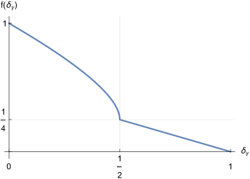
Figure 7: The function $f(\delta_{\gamma})$.

The last step is to minimize the rhs of the last inequality under the constraint of Eq. (77), that is

$$\min\quad \mathds{E}(f(\delta_{\gamma}))$$ (79)

such that $$\mathds{E}(\delta_{\gamma})\leq\varepsilon+\varepsilon_{*}$$ (80)

$$\delta_{\gamma}\geq\varepsilon_{*},$$ (81)

where the last line comes from $\text{Pr}(S_{\gamma})\leq\text{Pr}(G_{\gamma})\leq\text{Pr}(G_{*})=1-\varepsilon_{*}$. The function $f(\delta_{\gamma})$ is depicted in Fig. 7. We can relax this minimization to a trivial one if we find a convex decreasing lower bound on the goal function $f(\delta_{\gamma})\geq f_{\text{con}}(\delta_{\gamma})$ on the interval $\delta_{\gamma}\in[\varepsilon_{*},1]$, since such a function must satisfy

$$\mathds{E}(f(\delta_{\gamma}))\geq\mathds{E}(f_{\text{con}}(\delta_{\gamma}))\geq f_{\text{con}}(\mathds{E}(\delta_{\gamma}))\geq f_{\text{con}}(\varepsilon+\varepsilon_{*}).$$ (82)

Note that the function $f(\delta_{\gamma})$ is concave on the interval $[0,1/2]$, which follows from the negativity of its second derivative

$$f^{\prime\prime}(\delta_{\gamma})=-\frac{1}{2(1-2\delta_{\gamma})^{3/2}}<0.$$ (83)

It follows that a convex lower bound on the whole interval $\delta_{\gamma}\in[0,1]$ is provided by a linear function

$$f(\delta_{\gamma})\geq f_{\text{con}}(\delta_{\gamma})=1-\frac{3}{2}\delta_{\gamma},$$ (84)

which results in the following bound

$$\text{Pr}(\Upsilon)\geq\mathds{E}(f(\delta_{\gamma}))\geq 1-\frac{3}{2}(\varepsilon+\varepsilon_{*})\geq 1-3\varepsilon,$$ (85)

by $\varepsilon_{*}\leq\varepsilon$. In the next section we derive a tighter upper-bound which uses the fact that $\delta_{\gamma}\geq\varepsilon_{*}$.

A.1 Tighter bound on $\text{Pr}(\Upsilon)$

A tight convex lower bound on $f(\delta_{\gamma})$ depicted in Fig. 7 on the interval $[\varepsilon_{*},1]$ is given by the piece-wise linear function which connects connecting the points $\{\varepsilon_{*},f_{*}=f(\varepsilon_{*})\}$ with $\{1/2,1/4\}$ for $\delta_{\gamma}\in[\varepsilon_{*},1/2]$ and the points $\{1/2,1/4\}$ with $\{1,0\}$ for $\delta_{\gamma}\in[1/2,1]$. Formally, this lower bound is given by

$$f^{\varepsilon_{*}}_{\text{con}}(\delta_{\gamma})=\begin{cases}\frac{2f_{*}-\varepsilon_{*}}{2-4\varepsilon_{*}}-\frac{4f_{*}-1}{2-4\varepsilon_{*}}\delta_{\gamma}&\delta_{\gamma}\in[\varepsilon_{*},1/2]\\ \frac{1-\delta_{\gamma}}{2}&\delta_{\gamma}\in(1/2,1]\end{cases}$$ (86)

This implies a tight lower bound

$$\min\quad \mathds{E}(f(\delta_{\gamma}))\qquad\geq f^{\varepsilon_{*}}_{\text{con}}(\varepsilon+\varepsilon_{*})$$ (87)

such that $$\mathds{E}(\delta_{\gamma})\leq\varepsilon+\varepsilon_{*}$$ (88)

$$\delta_{\gamma}\geq\varepsilon_{*},$$ (89)

and $\text{Pr}(\Upsilon)\geq f^{\varepsilon_{*}}_{\text{con}}(\varepsilon+\varepsilon_{*})$ for any scenario with $\text{Pr}(G_{*})=1-\varepsilon_{*}$. But since $\varepsilon_{*}$ is not known we need to take the worst-case lower bound

$$\text{Pr}(\Upsilon)\geq 1-\text{f}_{\varepsilon}:=\min_{\varepsilon_{*}\in[0,\varepsilon]}f^{\varepsilon_{*}}_{\text{con}}(\varepsilon+\varepsilon_{*})$$ (90)

Finally, let us show that

$$1-\text{f}_{\varepsilon}=f^{\varepsilon}_{\text{con}}(2\varepsilon)=\begin{cases}\frac{1}{2}-\varepsilon+\frac{1-4\varepsilon}{2\sqrt{1-2\varepsilon}}&\varepsilon\leq\frac{1}{4}\\ \frac{1-2\varepsilon}{2}&\varepsilon>\frac{1}{4}\end{cases}$$ (91)

This follows from the fact that the function $f^{\varepsilon_{*}}_{\text{con}}(\varepsilon+\varepsilon_{*})$ is decreasing in $\varepsilon_{*}$ hence the minimum is reached by setting $\varepsilon_{*}=\varepsilon$. Indeed, its derivative

$$\frac{\partial}{\partial\varepsilon_{*}}f^{\varepsilon_{*}}_{\text{con}}(\varepsilon+\varepsilon_{*})=\begin{cases}-\frac{\left(1+\sqrt{1-2\varepsilon_{*}}\right)(1-2\varepsilon_{*})-2\varepsilon}{2(1-2\varepsilon_{*})^{3/2}}&\varepsilon+\varepsilon_{*}\leq\frac{1}{2}\\ -\frac{1}{2}&\varepsilon+\varepsilon_{*}>\frac{1}{2}\end{cases}$$ (92)

is negative. This concludes the proof of the lower bound

$$\text{Pr}(\Upsilon)\geq 1-\text{f}_{\varepsilon}\geq 1-3\varepsilon,$$ (93)

illustrated in Fig. 8. As a final remark consider the first order expansion $1-\text{f}_{\varepsilon}=1-\frac{5}{2}\varepsilon+O(\varepsilon^{2})$ to see that for very small $\varepsilon$ the two lower bounds are quite different.

Figure 8: The lower bounds $\text{f}_{\varepsilon}$ (full line) and $1-3\varepsilon$ (dashed line) on the probability $\text{Pr}(\Upsilon)$ of the PTC set as functions of the probability $\varepsilon=\text{Pr}(a\oplus b\oplus c\neq 1)$ to observe the wrong parity of the outcomes.

A.2 Solution of the optimization in Eq. (70)

Here we solve the optimization problem

$$\begin{split}\max_{p_{0},p_{1},q_{0},q_{1}}&\min\,\{p_{0}q_{0},p_{1}q_{1}\}\\ \text{such that}&\quad p_{0}+p_{1},q_{0}+q_{1}\leq 1\\ &\quad p_{0},p_{1},q_{0},q_{1}\geq 0\\ &\quad p_{0}q_{0}+p_{1}q_{1}\geq 1-\delta_{\gamma}.\end{split}$$ (94)

Without loss of generality consider the case $p_{0}q_{0}\leq p_{1}q_{1}$, and rewrite the problem as

$$\begin{split}\max_{p_{0},p_{1},q_{0},q_{1}}&\quad p_{0}q_{0}\\ \text{such that}&\quad p_{0}q_{0}\leq p_{1}q_{1}\\ &\quad p_{0}q_{0}\geq 1-\delta_{\gamma}-p_{1}q_{1}\\ &\quad p_{0}\leq 1-p_{1}\\ &\quad q_{0}\leq 1-q_{1}\\ &\quad p_{0},p_{1},q_{0},q_{1}\geq 0.\\ \end{split}$$ (95)

The variables $p_{1}$ and $q_{1}$ now do not appear in the goal function. Furthermore, the constraints on $p_{0}$ and $q_{0}$ are easier to satisfy, the larger values of $p_{1}$, $q_{1}$ and $p_{1}q_{1}$. Hence the maximum is attained when these auxiliary variables take the maximal values $p_{1}=1-p_{0}$ and $q_{1}=1-p_{0}$. This allows us to rewrite the maximization in terms of two variables $p=p_{0}$ and $q=q_{0}$ as follows

$$\begin{split}\max_{p,q\in[0,1]}&\quad p\,q\\ \text{such that}&\quad p\,q\leq(1-p)(1-q)\\ &\quad p\,q\geq 1-\delta_{\gamma}-(1-p)(1-q)\end{split}\qquad\text{or}\qquad\begin{split}\max_{p,q\in[0,1]}&\quad p\,q\\ \text{such that}&\quad p+q\leq 1\\ &\quad 2\,p\,q\geq p+q-\delta_{\gamma}\end{split}.$$ (96)

Let us introduce the variables $g=\sqrt{p\,q}$ and $a=\frac{p+q}{2}$ which are the geometric and the algebraic means of $p,q$. We there help we write

$$\begin{split}\max_{g,a}&\quad g^{2}\\ \text{such that}&\quad a\leq\frac{1}{2}\\ &\quad g^{2}\geq a-\frac{1}{2}\delta_{\gamma},\end{split}$$ (97)

and we also know that the algebraic and geometric means satisfy $a\geq g$, which can be saturated $a=g$ by the choice $p=q$. Note that for a fixed free variable $a$, the choice $g=a$ is the one that maximizes the goal function and relaxes the constraints the most. We can thus set $a=g$ without loss of generality in order to obtain

$$\begin{split}\max_{g\in[0,\frac{1}{2}]}&\quad g^{2}\\ \text{such that}&\quad g^{2}-g+\frac{1}{2}\delta_{\gamma}\geq 0.\end{split}$$ (98)

Here $g^{2}-g+\frac{1}{2}\delta_{\gamma}$ is a decreasing function of $g\in[0,1/2]$. It admits a zero at $g=\frac{1}{2}\left(1-\sqrt{1-2\delta_{\gamma}}\right)$ inside the interval, and is thus negative for larger values of $g$. We conclude that this is precisely the value maximizing $g$ and $g^{2}$ under the constraint. Hence, we have shown that

$$\begin{split}\max_{p_{0},p_{1},q_{0},q_{1}}&\min\,\{p_{0}q_{0},p_{1}q_{1}\}\qquad\quad=\left(\frac{1-\sqrt{1-2\,\delta_{\gamma}}}{2}\right)^{2}\\ \text{such that}&\quad p_{0}+p_{1},q_{0}+q_{1}\leq 1\\ &\quad p_{0},p_{1},q_{0},q_{1}\geq 0\\ &\quad p_{0}q_{0}+p_{1}q_{1}\geq 1-\delta_{\gamma}.\end{split}$$ (99)

Appendix B The noisy W-distribution

In this section, we illustrate Result 2 and discuss the nonlocality of noisy W-distributions. Such distributions $P_{W}^{(\varepsilon,\delta)}$ are given by

$$P_{W}^{(\varepsilon,\delta)}(100)=\frac{1-\varepsilon-\delta}{3}\circlearrowleft,\qquad P_{W}^{(\varepsilon,\delta)}(111)=\delta$$ (100)

and the other terms are left unspecified. It satisfies the PTC condition with probability $1-\varepsilon$. Hence, by our Result 2 we know that there must exist a local PTC distribution $P(a,b,c)$ such that $\delta(P_{W}^{(\varepsilon,\delta)},P)\leq\text{f}_{\varepsilon}$. With straightforward algebra, this condition can rewritten as

$$\Delta^{(\varepsilon,\delta)}(P)=\sum_{(a,b,c)=(100),(010),(001)}\left|\frac{1-\varepsilon-\delta}{3}-P(a,b,c)\right|+|\delta-P(111)|-2\text{f}_{\varepsilon}\leq 0.$$ (101)

Now, the set of the PTC distributions can be parameterized with the three “token probabilities” $p_{\xi}(0)=q_{\xi}\in[0,1]$ leading to

$$P(111) =q_{\alpha}q_{\beta}q_{\gamma}+(1-q_{\alpha})(1-q_{\beta})(1-q_{\gamma})$$ (102)

$$P(100) =(1-q_{\alpha})q_{\beta}q_{\gamma}+q_{\alpha}(1-q_{\beta})(1-q_{\gamma})\qquad\circlearrowleft.$$ (103)

Therefore the implication of result 2 is equivalent to

$$\Delta_{min}^{(\varepsilon,\delta)}=\min_{q_{\alpha},q_{\beta},q_{\gamma}}\Delta^{(\varepsilon,\delta)}(q_{\alpha}q_{\beta}q_{\gamma})\leq 0,$$ (104)

since there must exist a combination of $q_{\alpha},q_{\beta},q_{\gamma}$ for which $\Delta^{(\varepsilon,\delta)}(P)\leq 0$ holds. To prove that a distribution $P_{W}^{(\varepsilon,\delta)}$ is not triangle local it is thus sufficient to show that $\Delta_{min}^{(\varepsilon,\delta)}>0$.

Figure 9: In yellow we show the parameter region $(\varepsilon,\delta)$ where the noisy W-distributions $P_{W}^{(\varepsilon,\delta)}(a,b,c)$ in Eq. (100) appear to be nonlocal.

To perform the minimization in Eq. (104), we used the Nelder-Mead or simplex search method [30] via the Python library SciPy [31]. The results of the minimization are reported in Fig. 9. Note that this is an empirical minimization algorithm, which does not provide a convergence guarantee. Therefore, we have only proven the nonlocality of a given distribution under the assumption that the global minimum was found. Nevertheless, the goal function $\Delta^{(\varepsilon,\delta)}(q_{\alpha},q_{\beta},q_{\gamma})$ is a smooth and well-behaved function of three variables on a compact interval, and with more computational resources it is possible to do the minimization in a guaranteed manner, e.g. using a branch-and-bound algorithm.

Appendix C Linear Program for TBSM when PTC is satisfied exactly

Definition 1.

For a binary tuple of outputs $\bm{x}=(a,b,c)$, and a binary tuple of tokens $\bm{t}=(t_{\alpha},t_{\beta},t_{\gamma})$, we define the PTC response function as follows:

$$P_{\scriptscriptstyle PTC}(\bm{x}|\bm{t})=\begin{cases}1&a=t_{\beta}\oplus t_{\gamma}\oplus 1,\ b=t_{\gamma}\oplus t_{\alpha}\oplus 1\ ,c=t_{\alpha}\oplus t_{\beta}\oplus 1\\ 0&o.w.\end{cases}.$$

This function is indeed, an indicator function of whether the outputs $\bm{x}$ and tokens $\bm{t}$ are consistent. Note that clearly for any $\bm{t}$ there is only one consistent $\bm{x}$, and more interestingly for any PTC tuple $\bm{x}=(a,b,c)$, i.e. $a\oplus b\oplus c=1$, there are exactly two consistent tokens $\bm{t}$, which are flipped of each other. For example for $\bm{x}=(1,1,1)$ we find $\bm{t}=(1,1,1)$, or $\bm{t}=(0,0,0)$.

Noiseless case: nonlocality of $P(\bm{x}_{1}\bm{x}_{2})$ can be checked by the infeasibility of the following linear program with 8 probability distributions (64 variables) $P(\bm{x}_{2}|\bm{t})$ , where we use the compact notation $\bm{x}_{i}=(a_{i},b_{i},c_{i})$, $\bm{t}=(t_{\alpha},t_{\beta},t_{\gamma})$

$$\begin{split}&(i)\,P(\bm{x}_{1},\bm{x}_{2})=\sum_{\bm{t}}p(\bm{t})P_{\scriptscriptstyle PTC}(\bm{x}_{1}|\bm{t})P(\bm{x}_{2}|\bm{t})\\ &(ii)\ \sum_{b_{2},c_{2}}{P(a_{2},b_{2},c_{2}|0,t_{\beta},t_{\gamma})}-\sum_{b_{2},c_{2}}P(a_{2},b_{2},c_{2}|1,t_{\beta},t_{\gamma})=0\quad\circlearrowleft\end{split}$$ (105)

Note that as mentioned before, for any PTC tuple of $\bm{x}_{1}$, there are exactly two consistent $\bm{t}$, therefore the sum in $(i)$, is only over two terms.

Dephasing noise: the local dephasing noise given by the channel $\mathcal{E}_{d}:\outerproduct{\psi}{\psi}\mapsto\varrho$ with

$$\varrho=(1-d)\outerproduct{\psi}{\psi}+d\left(\lambda_{0}^{2}\outerproduct{01}{01}+\lambda_{1}^{2}\outerproduct{10}{10}\right)$$ (106)

where $\ket{\psi}=\lambda_{0}\ket{01}+\lambda_{1}\ket{10}$. Note that the resulting distribution $P$ in the presence of the dephasing noise is still a PTC distribution and can be written as

$$P=(1-d)^{3}P_{Q}+(1-(1-d)^{3})P_{C}$$

Where $P_{Q}$ is the quantum distribution obtained without the presence of dephasing noise($d=0$), and $P_{C}$ is the classical distribution($d=1$), therefore we have, $P=P_{Q}+(P_{C}-P_{Q})e$ for $e:=(1-(1-d)^{3})$ and using (105) finding the minimum amount of dephasing noise $d$ for which the distribution becomes local can be writen as

$$\text{Minimize \ }e$$ (107)

s.t. $$(i)\ P_{Q}(\bm{x}_{1}\bm{x}_{2})=\sum_{\bm{t}}{p(\bm{t})P_{\scriptscriptstyle PTC}(\bm{x}_{1}|\bm{t})P(\bm{x}_{2}|\bm{t})}+\big(P_{Q}(\bm{x}_{1}\bm{x}_{2})-P_{C}(\bm{x}_{1}\bm{x}_{2})\big)e$$ (108)

$$(ii)\ \sum_{b_{2},c_{2}}{P(a_{2},b_{2},c_{2}|0,t_{\beta},t_{\gamma})}-\sum_{b_{2},c_{2}}P(a_{2},b_{2},c_{2}|1,t_{\beta},t_{\gamma})=0\quad\circlearrowleft$$ (109)

Solving this LP, we find the optimum value $e^{*}$, which translates to the optimum dephasing noise $d^{*}=1+\sqrt[3]{e^{*}-1}$. We used MOSEK Optimizer API for Python to solve the Linear Program [32].

Appendix D Linear Program for noisy TBSM distributions

Lemma 1.

For probability distributions $p(x)$ and $q(x)$ the following statements are equivalent,

$$(i)\ \text{There exist probability distributions $p^{\prime}$ and $q^{\prime}$ such that }p(x)=q(x)+\varepsilon p^{\prime}(x)-\varepsilon q^{\prime}(x)$$

$$(ii)\ \delta_{TV}(p,q)\leq\varepsilon$$

Proof.

$(i)\Rightarrow(ii):$

$$\delta_{TV}(p,q)=\frac{1}{2}\sum_{x}|p(x)-q(x)|=\frac{\varepsilon}{2}\sum_{x}|p^{\prime}(x)-q^{\prime}(x)|=\varepsilon\ \delta_{TV}(p^{\prime},q^{\prime})\leq\varepsilon$$

$(ii)\Rightarrow(i):$ let’s define $r(x)=p(x)-q(x)$, then we have $\sum_{x}r(x)=0$ and $\sum_{x}|r(x)|\leq\varepsilon$ we define $p^{\prime}(x)=\frac{|r(x)|}{\sum_{x}|r(x)|}$ and $q^{\prime}(x)=p^{\prime}(x)-\frac{r(x)}{\varepsilon}$, which are valid probability distributions satisfying (i).

∎

LP for an observed distribution with $\text{Pr}\bm{(a_{1}\oplus b_{1}\oplus c_{1}=1)\geq 1-\varepsilon}$: Nonlocality of an observed distribution $P(\bm{x}_{1}\bm{x}_{2})$ can be checked by the infeasibility of the following quadratic constrained program with 6 probability distributions $P(\bm{x}_{2},\bm{t}),P^{\prime}(\bm{x}_{1},\bm{x}_{2}),\widetilde{P}^{\prime}(\bm{x}_{1},\bm{x}_{2}),p_{\alpha}(t),p_{\beta}(t),p_{\gamma}(t)$.

$$(*^{\prime})\,P(\bm{x}_{1},\bm{x}_{2})=\underbrace{\sum_{\bm{t}}P_{\scriptscriptstyle PTC}(\bm{x}_{1}|\bm{t})P(\bm{x}_{2},\bm{t})}_{\widetilde{P}(\bm{x}_{1}\bm{x}_{2})}-\text{f}_{\varepsilon}P^{\prime}(\bm{x}_{1},\bm{x}_{2})+\text{f}_{\varepsilon}\widetilde{P}^{\prime}(\bm{x}_{1},\bm{x}_{2})$$

$$(4.iii^{\prime})\,\sum_{\bm{x}_{1}}\widetilde{P}^{\prime}(\bm{x}_{1},\bm{x}_{2})=\sum_{\bm{x}_{1}}P^{\prime}(\bm{x}_{1},\bm{x}_{2})$$ (110)

$$(ii)\ p_{\alpha}(1)\sum_{b_{2},c_{2}}{P(a_{2},b_{2},c_{2},0,t_{\beta},t_{\gamma})}-p_{\alpha}(0)\sum_{b_{2},c_{2}}P(a_{2},b_{2},c_{2},1,t_{\beta},t_{\gamma})=0\quad\circlearrowleft$$ (111)

Note that $P(t_{\alpha},t_{\beta},t_{\gamma})=p_{\alpha}(t_{\alpha})p_{\beta}(t_{\beta})p_{\gamma}(t_{\gamma})$ is implied by the last constraint. Furthermore, this constraint is coming from the network structure which implies $P(a_{2}|0,t_{\beta},t_{\gamma})=P(a_{2}|1,t_{\beta},t_{\gamma})$. Moreover, note that here $p_{\alpha}(t),p_{\beta}(t),p_{\gamma}(t)$ correspond to the PTC distribution $\widetilde{P}$ and not the observed distribution $P$, therefore we do not know their values and we consider them as additional variables. Note that the quadratic constrains in $(iii)$ are not convex, i.e. if we write these constrains in the form of $x^{T}Qx$, the matrix $Q$ is not positive semidefinite.

Note that although we do not know the distributions $p_{\alpha}(t),p_{\beta}(t),p_{\gamma}(t)$ but we can bound them:

First notice that $p_{\alpha}(t_{\alpha}=0)=\frac{1}{2}\big(1+\sqrt{|\frac{\widetilde{E}_{b_{1}}\widetilde{E}_{c_{1}}}{\widetilde{E}_{a_{1}}}|}\big)$. Where, $\widetilde{E}_{x_{1}}=\widetilde{P}(x_{1}=0)-\widetilde{P}(x_{1}=1)$. It’s straightforward to see that the total variation distance leads to the conclusion that $|\widetilde{E}_{x_{1}}-E_{x_{1}}|\leq 2\text{f}_{\varepsilon}$. In fact, a slightly better bound can be obtained by using the fact that $\widetilde{P}$ is in the PTC slice, see section D.2 below,

$$|\widetilde{E}_{x_{1}}-E_{x_{1}}^{\Lambda}|\leq(2\text{f}_{\varepsilon}-\varepsilon),$$ (112)

where $E_{x_{1}}^{\Lambda}=P(x_{1}=0,a_{1}\oplus b_{1}\oplus c_{1}=1)-P(x_{1}=1,a_{1}\oplus b_{1}\oplus c_{1}=1)$ is computed from the PTC part of the observed distribution $P$. Hence, if all the correlators for the observed distribution satisfy $|E^{\Lambda}_{x_{1}}|\geq(2\text{f}_{\varepsilon}-\varepsilon)$ one can use Eq. (5) to obtain

$$\begin{split}l_{\alpha}:=\frac{1}{2}\left(1+\sqrt{\frac{(|E_{b_{1}}^{\Lambda}|-(2\text{f}_{\varepsilon}-\varepsilon))(|E_{c_{1}}^{\Lambda}|-(2\text{f}_{\varepsilon}-\varepsilon))}{|E_{a_{1}}^{\Lambda}|+(2\text{f}_{\varepsilon}-\varepsilon)}}\right)&\leq p_{\alpha}(0)\\ &\leq\frac{1}{2}\left(1+\sqrt{\frac{(|E_{b_{1}}^{\Lambda}|+(2\text{f}_{\varepsilon}-\varepsilon))(|E_{c_{1}}^{\Lambda}|+(2\text{f}_{\varepsilon}-\varepsilon))}{|E_{a_{1}}^{\Lambda}|-(2\text{f}_{\varepsilon}-\varepsilon)}}\right):=u_{\alpha}\quad\circlearrowleft.\end{split}$$ (113)

Therefore $(ii)$ can be written as:

$$\ l_{\alpha}\sum_{b_{2},c_{2}}{P(a_{2},b_{2},c_{2},0,t_{\beta},t_{\gamma})}-(1-l_{\alpha})\sum_{b_{2},c_{2}}P(a_{2},b_{2},c_{2},1,t_{\beta},t_{\gamma})\leq 0$$ (114)

$$\ u_{\alpha}\sum_{b_{2},c_{2}}{P(a_{2},b_{2},c_{2},0,t_{\beta},t_{\gamma})}-(1-u_{\alpha})\sum_{b_{2},c_{2}}P(a_{2},b_{2},c_{2},1,t_{\beta},t_{\gamma})\geq 0.$$ (115)

As an illustration, we can obtain bounds on the white noise robustness of the RGB4 distributions, see Fig. 10.

Figure 10: Noise robustness of the RGB4 distributions. Maximal amount of white noise below which we can prove the nonlocality of RGB4 distributions (TBSM distributions with $\phi_{w}=0$).

D.1 Collection of LPs (the grid technique for $p_{\xi}(t_{\xi})$)

Finally, note that the LP has to be satisfied for some values $p_{\xi}(t_{\xi})$ of the token probabilities in the intervals $[l_{\alpha},u_{\alpha}]$. In practice, it is convenient to divide each interval into smaller intervals $[l_{\alpha}+k\frac{u_{\alpha}-l_{\alpha}}{M},l_{\alpha}+(k+1)\frac{u_{\alpha}-l_{\alpha}}{M}]$, and verify that no solution can be found within any of the $M^{3}$ possible combinations of intervals. This gives a better result as compared to the harsher relaxation in Eqs. (114,115). In particular, for the figures 5,6,10,11, and 12 we used $M=16$, while to obtain the best bounds $\omega=0.544\%,\omega^{\prime}=0.504\%$ white noise and $\varepsilon=0.24\%$ total-variation distance we went to $M=128$.

Furthermore, to see how good is this relaxation of the $p_{\xi}(t_{\xi})$ variable to a finite set of intervals, we also check the feasibility of the LP for the honest values of $p_{\xi}(0)=q_{\xi}=\lambda_{0}^{2}$, i.e. the values which appear in the quantum strategy and are thus feasible by construction. This gives an upper bound on the maximum amount of noise for which the original feasibility problem could guarantee that the distribution is nonlocal.

D.2 Development of a tighter bound on $\widetilde{E}_{x_{1}}$

Note that we have:

$$P(\bm{x}_{1},\bm{\xi}\in\Lambda)=P(\bm{x}_{1},\bm{\xi}\in\Upsilon)+(\text{f}_{\varepsilon}-\varepsilon)P^{\prime\prime}(\bm{x}_{1})$$

$$\widetilde{P}(\bm{x}_{1})=P(\bm{x}_{1},\bm{\xi}\in\Upsilon)+\text{f}_{\varepsilon}\widetilde{P^{\prime}}(\bm{x}_{1})$$

Which can be rewritten as :

$$\widetilde{P}(\bm{x}_{1})=P(\bm{x}_{1},\bm{\xi}\in\Lambda)+\text{f}_{\varepsilon}\widetilde{P}^{\prime}(\bm{x}_{1})-(\text{f}_{\varepsilon}-\varepsilon)P^{\prime\prime}(\bm{x}_{1})$$

Therefore with $E_{x_{1}}^{\Lambda}=P(x_{1}=0,a_{1}\oplus b_{1}\oplus c_{1}=1)-P(x_{1}=1,a_{1}\oplus b_{1}\oplus c_{1}=1)$ we have

$$\widetilde{E}_{x_{1}}=E_{x_{1}}^{\Lambda}+\text{f}_{\varepsilon}\widetilde{E}^{\prime}_{x_{1}}-(\text{f}_{\varepsilon}-\varepsilon)E^{\prime\prime}_{x_{1}}$$

Therefore,

$$\widetilde{E}_{x_{1}}\in[E_{x_{1}}^{\Lambda}-(2\text{f}_{\varepsilon}-\varepsilon),E_{x_{1}}^{\Lambda}+(2\text{f}_{\varepsilon}-\varepsilon)].$$

Appendix E Other noise models

White noise at the measurement.

Alternatively to the white noise at the source, discussed in the main text, one can consider white noise affecting the measurements. In this case the POVM elements describing the measurement are replaced by

$$E_{x_{1},x_{2}}=(1-\omega^{\prime})\outerproduct{\phi_{x_1,x_2}}{\phi_{x_1,x_2}}+\omega^{\prime}\frac{\mathds{1}}{2}\otimes\frac{\mathds{1}}{2}.$$ (116)

Note that here for the resulting distribution we have $\text{Pr}(a_{1}\oplus b_{1}\oplus c_{1}=1)=\frac{1}{2}\left(1+(1-\omega^{\prime})^{3}\right)$. In Fig.  11(a), we depict the robustness to measurement white noise of the TBSM distributions with $\lambda_{0}^{2}=0.22$. The maximal amount of noise for which we can prove that nonlocality of the distribution is given by $\omega^{\prime}=0.504\%$ for the case $\phi_{u}=0.42$ and $\phi_{w}=0$.

Considering the combined effect of white noise at the sources and the parties we get, $\text{Pr}(a_{1}\oplus b_{1}\oplus c_{1}=1)=\frac{1}{2}\left(1+(1-\omega^{\prime})^{3}(1-\omega)^{3}\right)$. In Fig. 11(b), we depict the nonlocality of the TBSM distribution with $\phi_{u}=0.42$ and $\phi_{w}=0$ as a function of both the noise parameters.

(a) White noise at the masurement

(b) Noisy states and measurements

Figure 11: (a) Maximal amount of white noise at the level of measurements per party below which we can prove the nonlocality of the TBSM distribution. Parameters: $u=\cos(\phi_u)$, $w=\cos(\phi_w)$ and $\lambda_{0}^{2}=0.22$. (b) Noise robustness of the TBSM distribution when noise is added to both states ($\omega$) and measurements ($\omega^{\prime}$). The distribution is nonlocal in the yellow region, for parameters $\lambda_{0}^{2}=0.22,\phi_{u}=0.42,\phi_{w}=0$.

No-click noise.

Another natural imperfection to consider is the possibility that the measurement does not produce an outcome with probability $p$. This is described by five-outcome POVM given by

$$E_{x_{1},x_{2}} =(1-p)\outerproduct{\phi_{x_1,x_2}}{\phi_{x_1,x_2}}\qquad\forall x_{1},x_{2}=0,1$$ (117)

$$E_{\textup{\,\o\,}} =p\,\mathds{1}$$ (118)

where $E_{\textup{\,\o\,}}$ is the element associated with the no-click event. The probability distribution obtained with such measurements has five outcomes for each party and is not readily analyzed with the results presented in this paper. However, a trick commonly used for device-independent quantum key distribution is to relabel the no-click outcome to one of the four ”good” outcomes restoring output cardinality.

We find that the optimal strategy (for noise robustness) is for each party to relabel the no-click outcome to $\textup{\,\o\,}\to(1,0)$, which corresponds to the POVM

$$E_{1,0} =(1-p)\outerproduct{\phi_{1,0}}{\phi_{1,0}}+p\,\mathds{1}$$ (119)

$$E_{x_{1},x_{2}} =(1-p)\outerproduct{\phi_{x_1,x_2}}{\phi_{x_1,x_2}}\qquad\forall(x_{1},x_{2})\neq(1,0).$$ (120)

For this strategy, we prove the nonlocality of the resulting distribution for up to a no-click probability of $p=0.7\%$, see Fig.  12(a).

Note that if e.g. the sources produce two photons entangled in polarization $\ket{0}=\ket{1_h}$ and $\ket{1}=\ket{1_v}$, a limited photon transmission (or detector efficiency) $\eta$ would correspond to the no-click noise with $(1-p)=\eta^{2}$.

Single photon entanglement implementation with loss.

For $\phi_{w}=0$ the TBSM distributions (RGB4) can be realised with single-photon entanglement (vacuum state $\ket{0}$ and single photon $\ket{1}$), linear optics and photon number resolving detectors [28]. In this case the dominant noise is the limited efficiency of the detectors, which can be modeled as a photon loss channel with transmission $\eta$. Formally, we have the channel

$$\mathcal{E}(\rho) =K_{0}\rho K_{0}^{\dagger}+K_{1}\rho K_{1}^{\dagger}$$ (121)

$$K_{0} =\outerproduct{0}{0}+\sqrt{\eta}\outerproduct{1}{1}$$ (122)

$$K_{1} =\sqrt{1-\eta}\outerproduct{0}{1}$$ (123)

which is applied on all of the six modes. Alternatively, the noise can be absorbed in the measurements by considering the POVM elements

$$E_{x_{1},x_{2}}=\mathcal{E}^{*}\otimes\mathcal{E}^{*}(\Pi_{x_{1},x_{2}})=\sum_{i,j=0}^{1}K_{i}^{\dagger}\otimes K_{j}^{\dagger}\,\Pi_{x_{1},x_{2}}\,K_{i}\otimes K_{j}.$$ (124)

Recall that for $\phi_{w}=0$ the original projectors for $x_{1}=1$ read $\Pi_{00}=\outerproduct{00}{00}$ and $\Pi_{01}=\outerproduct{11}{11}$, while the lossy POVM elements read

$$E_{0,0} =\left(\begin{array}[]{cccc}1&0&0&0\\ 0&1-\eta&0&0\\ 0&0&1-\eta&0\\ 0&0&0&(1-\eta)^{2}\\ \end{array}\right)\qquad\qquad\quad E_{0,1}=\left(\begin{array}[]{cccc}0&0&0&0\\ 0&0&0&0\\ 0&0&0&0\\ 0&0&0&\eta^{2}\\ \end{array}\right)$$

$$E_{1,0} =\left(\begin{array}[]{cccc}0&0&0&0\\ 0&\eta u^{2}&\eta uv&0\\ 0&\eta uv&\eta v^{2}&0\\ 0&0&0&(1-\eta)\eta\\ \end{array}\right)\qquad E_{1,1}=\left(\begin{array}[]{cccc}0&0&0&0\\ 0&\eta v^{2}&-\eta uv&0\\ 0&-\eta uv&\eta u^{2}&0\\ 0&0&0&(1-\eta)\eta\\ \end{array}\right)$$

in the computational basis $\{\ket{00},\ket{01},\ket{10},\ket{11}\}$.

The nonlocality of the resulting distributions can be detected up to a transmission loss of $1-\eta=0.275\%$, see Fig. 12 (b).

(a) No-click scenario

(b) Single-photon entanglement scenario with loss

Figure 12: (a) Maximal no-click probability at each party below which we can prove the nonlocality of the distribution. Parameters: $u=\cos(\phi_u)$, $w=\cos(\phi_w)$ and $\lambda_{0}^{2}=0.22$. (b) Maximal amount of photon loss at measurements below which we can prove the nonlocality of the RGB4 distribution (TBSM with $\phi_{w}=0$) for the single-photon entanglement implementation. Here $\eta$ denotes the detection efficiency, i.e. the probability that an emitted photon is detected. Parameters: $u=\cos(\phi_u)$, $\phi_{w}=0$ and $\lambda_{0}^{2}=0.22$

Appendix F Linear Program for the total variation distance

Given a target quantum distribution $\bar{P}(\bm{x}_{1},\bm{x}_{2})\in\mathcal{Q}_{\triangle}^{4}$ define the total variation distance ball as the following subset of the correlation set

$$\mathcal{B}_{\varepsilon}(\bar{P})=\{P\in\mathcal{P}_{\triangle}^{4}|\delta(P,\bar{P})\leq\varepsilon\}.$$ (141)

We will now demonstrate that for well-chosen target distributions $\bar{P}$ and small enough $\varepsilon$ the entire set $\mathcal{B}_{\varepsilon}(\bar{P})$ is nonlocal. Concretely, consider $\bar{P}$ such that $a_{1}\oplus b_{1}\oplus c_{1}=1$. Any distribution $P\in\mathcal{B}_{\varepsilon}(\bar{P})$ must satisfy

$$\text{Pr}(a_{1}\oplus b_{1}\oplus c_{1}=1)\geq 1-\varepsilon.$$ (142)

We will prove that all distributions in $\mathcal{B}_{\varepsilon}(\bar{P})$ are nonlocal by contradiction. Let us assume that the ball contains some triangle local distribution $P$, then from Result 3 there must exist a local PTC distribution $\widetilde{P}$ with $\delta(\widetilde{P}(\bm{x}_{1},\bm{x}_{2}),P(\bm{x}_{1},\bm{x}_{2}))\leq\text{f}_{\varepsilon}$ and $\delta(\widetilde{P}(\bm{x}_{2}),P(\bm{x}_{2}))=0$. By triangle inequality, $\widetilde{P}$ must also satisfy

$$\delta(\widetilde{P}(\bm{x}_{1},\bm{x}_{2}),\bar{P}(\bm{x}_{1},\bm{x}_{2})) \leq\delta(\widetilde{P},P)+\delta(P,\bar{P})\leq\varepsilon+\text{f}_{\varepsilon}$$ (143)

$$\delta(\widetilde{P}(\bm{x}_{2}),\bar{P}(\bm{x}_{2})) \leq 0+\delta(P,\bar{P})\leq\varepsilon.$$ (144)

Therefore, from Eq. (143) and Lemma 1

$$\bar{P}(\bm{x}_{1},\bm{x}_{2})=\underbrace{\sum_{\bm{t}}P_{\scriptscriptstyle PTC}(\bm{x}_{1}|\bm{t})P(\bm{x}_{2},\bm{t})}_{\widetilde{P}(\bm{x}_{1}\bm{x}_{2})}-(\varepsilon+\text{f}_{\varepsilon})\bar{P}^{\prime}(\bm{x}_{1},\bm{x}_{2})+(\varepsilon+\text{f}_{\varepsilon})\widetilde{P}^{\prime}(\bm{x}_{1},\bm{x}_{2})$$ (145)

Taking the marginal we get

$$\bar{P}(\bm{x}_{2})=\widetilde{P}(\bm{x}_{2})-(\varepsilon+\text{f}_{\varepsilon})\bar{P}^{\prime}(\bm{x}_{2})+(\varepsilon+\text{f}_{\varepsilon})\widetilde{P}^{\prime}(\bm{x}_{2})$$ (146)

Now from this equation and Eq. (144) we get

$$\delta(\widetilde{P}^{\prime}(\bm{x}_{2}),\bar{P}^{\prime}(\bm{x}_{2}))=\frac{1}{\varepsilon+\text{f}_{\varepsilon}}\delta(\widetilde{P}(\bm{x}_{2}),\bar{P}(\bm{x}_{2}))\leq\frac{\varepsilon}{\varepsilon+\text{f}_{\varepsilon}}:=\alpha$$ (147)

Note that as $2.5\varepsilon\leq\text{f}_{\varepsilon}\leq 3\varepsilon$, we have $1/4\leq\alpha\leq 2/7$, moreover for small values of $\varepsilon$, we have $\text{f}_{\varepsilon}\approx 2.5\varepsilon$ and $\alpha\approx 2/7$. Again by Lemma 1, we have

$$(4.iii^{\prime})\,\sum_{\bm{x}_{1}}\widetilde{P}^{\prime}(\bm{x}_{1},\bm{x}_{2})-\sum_{\bm{x}_{1}}\bar{P}^{\prime}(\bm{x}_{1},\bm{x}_{2})+\alpha\widetilde{P}^{\prime\prime}(\bm{x}_{2})-\alpha\bar{P}^{\prime\prime}(\bm{x}_{2})=0$$ (148)

Moreover, like before, we use the network constraint that $P(a_{2}|0,t_{\beta},t_{\gamma})=P(a_{2}|1,t_{\beta},t_{\gamma})$ written as the following

$$(ii)\ p_{\alpha}(0)\sum_{b_{2},c_{2}}{P(a_{2},b_{2},c_{2},0,t_{\beta},t_{\gamma})}-p_{\alpha}(1)\sum_{b_{2},c_{2}}P(a_{2},b_{2},c_{2},1,t_{\beta},t_{\gamma})=0\quad\circlearrowleft$$ (149)

Note that here $p_{\alpha}(t),p_{\beta}(t),p_{\gamma}(t)$ correspond to the PTC distribution $\widetilde{P}$ which is not observed, but we can bound $p_{\alpha}(t),p_{\beta}(t),p_{\gamma}(t)$:

Notice that $p_{\alpha}(t_{\alpha}=0)=\frac{1}{2}\big(1+\sqrt{|\frac{\widetilde{E}_{b_{1}}\widetilde{E}_{c_{1}}}{\widetilde{E}_{a_{1}}}|}\big)$. Where, $\widetilde{E}_{x_{1}}=\widetilde{P}(x_{1}=0)-\widetilde{P}(x_{1}=1)$. It’s straightforward to see that the total variation distance $\delta(\widetilde{P},\bar{P})\leq\text{f}_{\varepsilon}+\varepsilon$, leads to the conclusion that $|\widetilde{E}_{x_{1}}-\bar{E}_{x_{1}}|\leq 2(\text{f}_{\varepsilon}+\varepsilon)$. Where $\bar{E}_{x_{1}}=\bar{P}(x_{1}=0)-\bar{P}(x_{1}=1)$ is computed from the target PTC distribution $\bar{P}$. Hence, if all the correlators for the target distribution satisfy $|\bar{E}_{x_{1}}|\geq 2(\text{f}_{\varepsilon}+\varepsilon)$ one can use Eq. (5) to obtain

$$\begin{split}l_{\alpha}:=\frac{1}{2}\left(1+\sqrt{\frac{(|\bar{E}_{b_{1}}|-2(\text{f}_{\varepsilon}+\varepsilon))(|\bar{E}_{c_{1}}|-2(\text{f}_{\varepsilon}+\varepsilon))}{|\bar{E}_{a_{1}}|+2(\text{f}_{\varepsilon}+\varepsilon)}}\right)\leq\ p_{\alpha}(0)\ \leq\frac{1}{2}\left(1+\sqrt{\frac{(|\bar{E}_{b_{1}}|+2(\text{f}_{\varepsilon}+\varepsilon))(|\bar{E}_{c_{1}}|+2(\text{f}_{\varepsilon}+\varepsilon))}{|\bar{E}_{a_{1}}|-2(\text{f}_{\varepsilon}+\varepsilon)}}\right):=u_{\alpha}\quad\circlearrowleft.\end{split}$$ (150)

Therefore $(ii)$ can be written as:

$$\begin{split}\ l_{\alpha}\sum_{b_{2},c_{2}}{P(a_{2},b_{2},c_{2},0,t_{\beta},t_{\gamma})}-(1-l_{\alpha})\sum_{b_{2},c_{2}}P(a_{2},b_{2},c_{2},1,t_{\beta},t_{\gamma})\leq 0\\ \ u_{\alpha}\sum_{b_{2},c_{2}}{P(a_{2},b_{2},c_{2},0,t_{\beta},t_{\gamma})}-(1-u_{\alpha})\sum_{b_{2},c_{2}}P(a_{2},b_{2},c_{2},1,t_{\beta},t_{\gamma})\geq 0\end{split}$$ (151)

Combining Equations 145, 148 151, we get a set of linear constraints which should be satisfied if there exists any local distribution inside the ball $\mathcal{B}_{\varepsilon}(\bar{P})$. Therefore, the infeasibility of this LP, proves the non-locality of all of the points in $\mathcal{B}_{\varepsilon}(\bar{P})$. (See Fig.  6). Again to find tighter bounds we use the grid technique.