ALMA Observations of Supernova Remnant N49 in the Large Magellanic Cloud.
II. Non-LTE Analysis of Shock-heated Molecular Clouds

Abstract

We present the first compelling evidence of shock-heated molecular clouds associated with the supernova remnant (SNR) N49 in the Large Magellanic Cloud (LMC). Using ¹²CO($J$ = 2–1, 3–2) and ¹³CO($J$ = 2–1) line emission data taken with the Atacama Large Millimeter/Submillimeter Array, we derived the H₂ number density and kinetic temperature of eight ¹³CO-detected clouds using the large velocity gradient approximation at a resolution of $3\farcs 5$ ($\sim$0.8 pc at the LMC distance). The physical properties of the clouds are divided into two categories: three of them near the shock front show the highest temperatures of $\sim$50 K with densities of $\sim$500–700 cm^-3, while other clouds slightly distant from the SNR have moderate temperatures of $\sim$20 K with densities of $\sim$800–1300 cm^-3. The former clouds were heated by supernova shocks, but the latter were dominantly affected by the cosmic-ray heating. These findings are consistent with the efficient production of X-ray recombining plasma in N49 due to thermal conduction between the cold clouds and hot plasma. We also find that the gas pressure is roughly constant except for the three shock-engulfed clouds inside or on the SNR shell, suggesting that almost no clouds have evaporated within the short SNR age of $\sim$4800 yr. This result is compatible with the shock-interaction model with dense and clumpy clouds inside a low-density wind bubble.

1 Introduction

Supernova remnants (SNRs) have a significant influence on the interstellar medium (ISM) via supernova shocks, injection of heavy elements, and cosmic-ray acceleration. In particular, shock heating and compression of a gaseous medium play an essential role not only in the evolution of the ISM but also in regulating both star formation and the structural evolution of galaxies (e.g., Inutsuka et al., 2015; Körtgen et al., 2016). Several pioneering observations have shown evidence of shock-heated molecular clouds at dozens of kelvins in the vicinity of Galactic SNRs using the non-local thermodynamic equilibrium (non-LTE) approximation (e.g., Cornett et al., 1977; White et al., 1987). Seta et al. (1998) presented enhanced ¹²CO $J$ = 2–1/1–0 intensity ratios of $\gtrsim$ 1–3 in shocked molecular clouds in Galactic SNRs W44 and IC 443, and derived typical kinetic temperatures of $\sim$40–80 K in these clouds. Subsequent molecular-line observations also established the presence of supernova-shocked warm clouds using non-LTE codes, and discussed their relation to star formation and/or high-energy phenomena (e.g., Reach & Rho, 1999; Anderl et al., 2014; Rho et al., 2015, 2017; Hogge et al., 2019; Sano et al., 2021b, a; Mazumdar et al., 2022). More recently, an unusually high HCO⁺/CO ratio has also been observed in molecular clouds interacting with SNRs, possibly due to high cosmic-ray ionization rates (Zhou et al., 2022). On the other hand, there have been no such studies on extragalactic SNRs especially in the Large Magellanic Cloud (LMC), despite the advantages of very little contamination along the line of sight (a small inclination angle of the LMC disk $\sim$20^∘–30^∘, e.g., Subramanian & Subramaniam, 2010) and its known distance ($\sim$$50\pm 1.3$ kpc, Pietrzyński et al., 2013).

LHA 120-N49 (hereafter N49) in the LMC is one of the best extragalactic SNRs to study shock-heating and compression of a gaseous medium because it is believed to be associated with molecular clouds (e.g., Banas et al., 1997; van Loon et al., 2010b; Uchida et al., 2015). The bright radio shell of N49 with centrally filled thermal X-rays is a typical characteristic of a mixed-morphology SNR (Rho & Petre, 1998). Although N49 has an apparent diameter of only $\sim$$75^{\prime\prime}$ (or $\sim$18.2 pc, see Bozzetto et al., 2017), Chandra resolved its filamentary diffuse emission and bright knots of X-rays at a resolution of $\sim$0$\farcs$5 (e.g., Park et al., 2003, 2012). The Sedov age of N49 was estimated to $\sim$4800 yr (Park et al., 2012). The nearby star-forming activity and spectral characteristics of the SNR generally support a massive progenitor star for N49 (Klose et al., 2004; Badenes et al., 2009; Yamaguchi et al., 2014). The projection of the magnetar candidate SGR 0526$-$66 within the boundary of N49 may support a core-collapse origin for N49, although the physical association between N49 and SGR 0526$-$66 is not conclusive (e.g., Gaensler et al., 2001; Park et al., 2012). Thus, while the Type Ia origin may not be completely ruled out based on the Si/S ejecta abundance ratio (e.g., Park et al., 2012), a core-collapse origin from the explosion of a massive progenitor is generally considered for N49.

A giant molecular cloud (GMC) in the N49 region was first discovered by Banas et al. (1997) using the ¹²CO($J$ = 2–1) emission line with the Swedish-ESO Submillimeter Telescope at a resolution of $\sim$$23^{\prime\prime}$ or $\sim$5.5 pc. The GMC has a diameter of $\sim$14 pc and lies on the southeastern shell of N49, in the direction in which the SNR is brightest in both the radio continuum and X-rays. The authors concluded that the GMC is possibly associated with the SNR. Subsequent Mopra observations using the ¹²CO($J$ = 1–0) emission line also supported this idea (Sano et al., 2017a). An important breakthrough came from observations of the ¹²CO($J$ = 1–0) emission line by Yamane et al. (2018) (hereafter Paper I, ) using the Atacama Large Millimeter/Submillimeter Array (ALMA). Thanks to the high angular resolution of ALMA of $3\farcs 2\times 2\farcs 3$ (or 0.78 pc $\times$ 0.56 pc), the GMC was resolved into 21 molecular clouds. At least three of them are limb-brightened on sub-parsec scales in both hard X-rays and radio continuum, suggesting shock-cloud interactions (e.g., Inoue et al., 2009, 2012; Sano et al., 2010).

In this paper, we derive the H₂ number density and kinetic temperature of molecular clouds in the vicinity of the SNR N49 using ALMA observations of ¹²CO($J$ = 1–0, 2–1, 3–2) and ¹³CO($J$ = 2–1) and a non-LTE analysis. Our findings for the shock- and/or cosmic-ray-heated clouds provide a new perspective on the ISM surrounding extragalactic SNRs for the first time. In Section 2, we present the observational details and data reduction of the ALMA CO data as well as archival X-ray data. Section 3 gives an overview of CO distributions and their physical properties. In Sections 4 and 5 we discuss and summarize our findings.

2 Observations and Data Reduction

2.1 ALMA CO

We carried out observations of ¹²CO($J$ = 3–2) emission line using the ALMA Atacama Compact Array Band 7 in Cycle 8 (PI: Hidetoshi Sano, #2021.2.00008.S). We used 10–11 antennas of the 7 m array in 2022 August 22, 27, 30, and September 2. We also used 3–4 antennas of the Total Power (TP) array in 2022 August 2, 4, 7, 8, 13, 17, 18, 20, and 27. The effective observed area was an approximately $1\farcm 2\times 1\farcm 3$ rectangular region centered at ($\alpha_{\mathrm{J2000}}$, $\delta_{\mathrm{J2000}})=(05^{\mathrm{h}}26^{\mathrm{m}}04\fs 82$, $-66\arcdeg 05\arcmin 23\fs 8$). The baseline range of the 7 m array was from 8.9 to 91.0 m, corresponding to $u$–$v$ distances from 10.2 to 105.0 $k\lambda$ at 345.796 GHz. Bandpass and flux calibration were carried out using quasar J0538$-$4405 and we used quasar J0601$-$7036 as a phase calibrator.

Observations of ¹²CO($J$ = 2–1) and ¹³CO($J$ = 2–1) emission lines were carried out using ALMA Band 6 in Cycle 3 (PI: Jacco Th. van Loon, #2015.1.01195.S). We used 45–46 antennas of the 12 m array in 2016 January 27 and 28; 8–10 antennas of the 7 m array in 2016 August 30, 31, September 2, and 4. The effective observed area was an approximately $1^{\prime}\times 1^{\prime}$ rectangular region centered at ($\alpha_{\mathrm{J2000}}$, $\delta_{\mathrm{J2000}})=(05^{\mathrm{h}}26^{\mathrm{m}}04\fs 00$, $-66\arcdeg 05\arcmin 20\fs 0$). The combined baseline range of the 12 and 7 m arrays was from 8.9 to 331.0 m, corresponding to $u$–$v$ distances from 6.8 to 254.5 $k\lambda$ at 230.538 GHz. The bandpass calibration was carried out by observing three quasars J0519$-$4546, J0522$-$3627, and J0006$-$0623. Another two quasars, J0529$-$7245 and J0601$-$7036, were observed as phase calibrators. We also used Uranus, J0538$-$4405, and J0601$-$7036 as flux calibrators.

Data reduction and imaging were performed using the Common Astronomy Software Applications package (CASA, version 5.4.1; CASA Team et al., 2022). We applied the multiscale CLEAN algorithm with the natural weighting scheme (Cornwell, 2008). Here we used the tclean task to make the images. We then combined the cleaned 7 m data and the calibrated TP array data for CO($J$ = 3–2) and the cleaned 12 and 7 m array data for CO($J$ = 2–1) using the feather task. The final beam size of the feathered image was $3\farcs 48\times 2\farcs 76$ with a position angle of 33$\fdg$7 for the ¹²CO($J$ = 3–2) emission line; $1\farcs 73\times 1\farcs 10$ with a position angle of 76$\fdg$7 for the ¹²CO($J$ = 2–1) emission line; and $1\farcs 82\times 1\farcs 14$ with a position angle of 77$\fdg$0 for the ¹³CO($J$ = 2–1) emission line. The typical RMS noise was $\sim$0.11 K at a velocity resolution of 0.4 km s^-1 for the ¹²CO($J$ = 3–2) emission line, and $\sim$0.09 K at a velocity resolution of 0.4 km s^-1 for both the ¹²CO($J$ = 2–1) and ¹³CO($J$ = 2–1) emission lines. The primary beam correction was applied with a threshold of 0.2 for ¹²CO($J$ = 2–1) and 0.5 for ¹²CO($J$ = 3–2) and ¹³CO($J$ = 2–1).

In order to take an intensity ratio of two different CO $J$-transitions, we also used the primary-beam-corrected, ¹²CO($J$ = 1–0) cleaned data published in Paper I. The beam size was $3\farcs 19\times 2\farcs 25$ with a position angle of 66$\fdg$14. The typical RMS noise was $\sim$0.07 K at a velocity resolution of 0.4 km s^-1.

2.2 Chandra X-Rays

We utilized archival X-ray data obtained by Chandra with the Advanced CCD Imaging Spectrometer S-array (ACIS-S3). The observation IDs were 747, 1041, 1957, 2515, 10123, 10806, 10807, and 10808, and were published in previous papers (Park et al., 2003, 2012, 2020; Yamane et al., 2018; Zhou et al., 2019). We utilized Chandra Interactive Analysis of Observations software (CIAO version 4.12; Fruscione et al., 2006) with CALDB 4.9.1 (Graessle et al., 2007) for the data reduction. All of the data were reprocessed using the task chandra_repro. The total effective exposure reached $\sim$197 ks for the eastern rim of the SNR, where the shock-cloud interactions occur. We then made an exposure-corrected, energy-filtered image using the task fluximage in the energy band of 0.5–7.0 keV as a broad-band X-ray image.

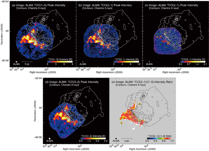
Figure 1: Peak intensity maps of (a) ¹²CO($J$ = 1–0), (b) ¹²CO($J$ = 2–1), (c) ¹³CO($J$ = 2–1), and (d) ¹²CO($J$ = 3–2). (e) Intensity ratio map of ¹²CO($J$ = 2–1)/¹²CO($J$ = 1–0) (hereafter $R_{\mathrm{2-1/1-0}}$). The velocity range of CO is from 285.5 to 287.8 km s^-1. Superposed contours represent Chandra X-ray intensity in the energy band of 0.5–7.0 keV. The lowest contour level and the contour intervals are $5\times 10^{-7}$ and $3\times 10^{-6}$ photons pixel^-1 s^-1, respectively. The regions enclosed by dashed lines indicate the observed areas using ALMA. The CO peaks K, L, N, O–R, and T defined by Paper I are also indicated in (c). When we take the intensity ratio of $R_{\mathrm{2-1/1-0}}$, the ¹²CO($J$ = 2–1) data were smoothed with a two-dimensional Gaussian kernel to match the effective beam size of the ¹²CO($J$ = 1–0) data. The gray shaded area in (e) represents the ¹²CO($J$ = 1–0) and/or ¹²CO($J$ = 2–1) data showing significance lower than $\sim$10$\sigma$.

3 Results

3.1 Distributions of CO and X-Rays

Figures 1a–1d show the peak intensity maps of ¹²CO($J$ = 1–0), ¹²CO($J$ = 2–1), ¹³CO($J$ = 2–1), and ¹²CO($J$ = 3–2) at $V_{\mathrm{LSR}}=285.5$–287.8 km s^-1, corresponding to the shocked components in N49 (Paper I). The clouds detected in ¹²CO($J$ = 2–1) and ¹²CO($J$ = 3–2) are situated along the southeastern edge of the X-ray shell and their spatial distribution is consistent with that seen in ¹²CO($J$ = 1–0) in Paper I.

In comparison to ¹²CO, the ¹³CO clouds are distributed more sparsely (see Figure 1c). Generally, in the LMC, both pre-star formation and active star-forming clouds exhibit relatively similar distributions for ¹²CO and ¹³CO (e.g., Wong et al., 2019), often forming prominent filamentary structures (e.g., Fukui et al., 2019; Tokuda et al., 2019). The compact, peculiar nature of the ¹³CO distribution in N49 is distinct from the above-mentioned interstellar trends, and unique to this SNR. Eight of them, K, L, N, O–R, and T, are detected in ¹³CO($J$ = 2–1) with $3\sigma$ or higher significance. The fundamental physical properties of ¹³CO-detected clouds (position, brightness temperature, center velocity, spectral linewidth, cloud size, virial mass) are summarized in Table 1. In the present paper, we focus on these clouds to estimate their kinetic temperature and H₂ number density.

Table 1: Physical Properties of ¹³CO Detected Clouds in SNR N49

Name	$\alpha_{\mathrm{J2000}}$	$\delta_{\mathrm{J2000}}$	$T_{\mathrm{b}}$			$V_{\mathrm{peak}}$	$\bigtriangleup V$	Size	$M_{\mathrm{vir}}$	$R_{\mathrm{dist}}$	$T_{\mathrm{kin}}$	$n$(H2)
			12CO(3–2)	12CO(2–1)	13CO(2–1)
	(h m s)	(∘ ′ ′′)	(K)	(K)	(K)	(km $\mathrm{s^{-1}}$)	(km $\mathrm{s^{-1}}$)	(pc)	($M_{\sun}$)	(pc)	(K)	($10^{3}$ cm-3)
(1)	(2)	(3)	(4)	(5)	(6)	(7)	(8)	(9)	(10)	(11)	(12)	(13)
K ……	5$:$26$:$5.5	$-$66$:$05$:$21	$3.60$	$6.59$	$0.35$	$285.5$	$0.83$	1.3	080	10.7	$45^{+14}_{-9\phantom{0}}$	$0.53^{+0.05}_{-0.06}$
L ……	5$:$26$:$4.7	$-$66$:$05$:$02	$2.00$	$3.75$	$0.18$	$286.3$	$1.72$	1.2	340	07.7	$42^{+26}_{-13}$	$0.72^{+0.13}_{-0.14}$
N ……	5$:$26$:$6.7	$-$66$:$05$:$15	$2.58$	$4.67$	$0.40$	$286.4$	$0.40$	0.8	010	11.6	$21^{+4\phantom{0}}_{-3\phantom{0}}$	$0.78^{+0.02}_{-0.04}$
O ……	5$:$26$:$3.7	$-$66$:$05$:$23	$4.91$	$8.26$	$0.91$	$286.2$	$0.69$	1.2	050	08.8	$19^{+1\phantom{0}}_{-2\phantom{0}}$	$1.10^{+0.01}_{-0.01}$
P ……	5$:$26$:$7.5	$-$66$:$05$:$12	$2.17$	$3.70$	$0.36$	$286.4$	$1.00$	1.1	100	12.2	$19^{+4\phantom{0}}_{-3\phantom{0}}$	$1.32^{+0.01}_{-0.03}$
Q ……	5$:$26$:$1.7	$-$66$:$05$:$34	$1.82$	$3.64$	$0.25$	$286.5$	$0.90$	1.0	080	09.6	$21^{+6\phantom{0}}_{-4\phantom{0}}$	$0.81^{+0.06}_{-0.05}$
R ……	5$:$26$:$6.3	$-$66$:$05$:$11	$3.17$	$5.49$	$0.51$	$286.4$	$0.86$	1.1	080	10.7	$20^{+3\phantom{0}}_{-2\phantom{0}}$	$1.10^{+0.02}_{-0.03}$
T ……	5$:$26$:$1.0	$-$66$:$05$:$27	$1.55$	$2.94$	$0.14$	$286.4$	$0.57$	0.9	030	07.7	$46^{+57}_{-18}$	$0.48^{+0.09}_{-0.14}$

Note. — Col. (1): Cloud name defined by Paper I. Cols. (2, 3): Position of the maximum intensity of ¹²CO($J$ = 1–0) ( Paper I, ). Cols. (4–8): Physical properties of CO emission derived from a single Gaussian fitting. All the CO datasets were smoothed to match the beam size of $3\farcs 5\times 3\farcs 5$. Cols. (4–6): Peak brightness temperature of ¹²CO($J$ = 3–2), ¹²CO($J$ = 2–1), and ¹³CO($J$ = 2–1) emision. Col. (7): Central velocity of ¹³CO($J$ = 2–1) spectra, $V_{\mathrm{peak}}$. Col. (8): Full-width at half-maximum (FWHM) line width of ¹³CO($J$ = 2–1) spectra, $\bigtriangleup V$. Col. (9): ¹³CO($J$ = 2–1) derived cloud size defined as ($A$/$\pi$)^0.5 $\times 2$, where $A$ is the total cloud surface area surrounded by the half intensity of peak integrated intensity contour. Col. (10): Mass of the cloud derived using the virial theorem and ¹³CO($J$ = 2–1) properties, $M_{\mathrm{vir}}$. Col. (11): Radial distance from the geometric center of the SNR at ($\alpha_{\mathrm{J2000}}$, $\delta_{\mathrm{J2000}})=(5^{\mathrm{h}}25^{\mathrm{m}}59\fs 57$, $-66\arcdeg 04\arcmin 56\fs 4$). Col. (12): Kinetic temperature, $T_{\mathrm{kin}}$. Col. (12): Number density of molecular hydrogen, $n$(H₂).

3.2 Intensity Ratio of ¹²CO($J$ = 2–1)/¹²CO($J$ = 1–0)

Figure 1e shows the intensity ratio distribution of ¹²CO($J$ = 2–1)/¹²CO($J$ = 1–0) (hereafter $R_{\mathrm{2-1/1-0}}$). The intensity ratio is a good indicator of the degree of the CO rotational excitation because the $J$ = 2 level is at an excitation energy of $E/k=16.5$ K, $\sim$10 K above the $J$ = 1 level at $E/k=5.5$ K (e.g., Seta et al., 1998). We find a high intensity ratio of $R_{\mathrm{2-1/1-0}}$ $\sim$1.0–1.2 in the entire molecular cloud associated with the SNR. We also confirmed that the intensity ratio distribution of ¹²CO($J$ = 3–2)/¹²CO($J$ = 1–0) is similar to that of $R_{\mathrm{2-1/1-0}}$. It is noteworthy that no extra heating sources such as OB stars and/or young stellar objects are associated with the molecular clouds in the vicinity of the SNR.

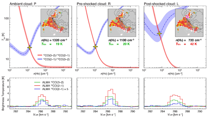
Figure 2: Top panels: large velocity gradient results on the number density of molecular hydrogen, $n$(H₂), and the kinetic temperature, $T_{\mathrm{kin}}$, for the ambient cloud P, pre-shocked cloud R, and the post-shocked cloud L. The red lines and blue dashed-dotted lines indicate the intensity ratios of ¹²CO($J$ = 3–2)/¹²CO($J$ =2–1) and ¹³CO($J$ = 2–1)/¹²CO($J$ =3–2), respectively. The shaded areas surrounding the red and blue lines indicate the $1\sigma$ ranges of each intensity ratio. Yellow crosses represent the best-fit values of $n$(H₂) and $T_{\mathrm{kin}}$ for each cloud. The spatial positions and best-fit values for each cloud are shown in the top-right corners for each panel. Bottom panels: CO intensity profiles for clouds P, R, and L. The physical properties of each cloud are summarized in Table 1.

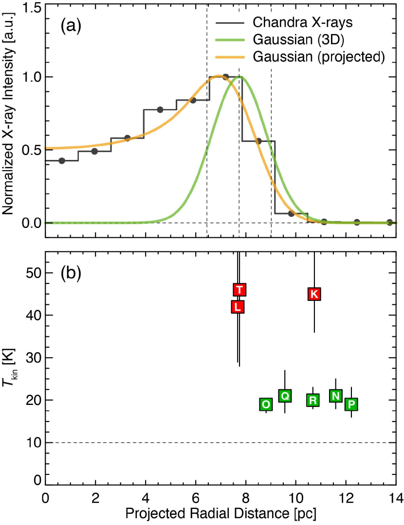
Figure 3: (a) Radial profile of the normalized X-ray intensity, centered at ($\alpha_{\mathrm{J2000}}$, $\delta_{\mathrm{J2000}})=(05^{\mathrm{h}}25^{\mathrm{m}}59\fs 57$, $-66\arcdeg 04\arcmin 56\fs 4$) as the geometric center of the SNR. The steps with filled circles indicate averaged values of normalized X-ray intensity at each annulus. The green line indicates the three-dimensional Gaussian distribution, and the orange line represents its projected distribution given by the least-squares fitting (see the text). (b) Scatter plot of kinetic temperature $T_{\mathrm{kin}}$ for each cloud as a function of the projected radial distance. The dashed horizontal line represents $T_{\mathrm{kin}}$ = 10 K, coresponding to the typical temperature of quiescent molecular clouds. The red and green symbols represent high- and moderate temperature clouds, respectively.

3.3 Large Velocity Gradient Analysis

In order to estimate the kinetic temperature $T_{\mathrm{kin}}$ and H₂ number density $n$(H₂) of molecular clouds in N49, we performed a non-LTE analysis using the large velocity gradient (LVG) approximation (e.g., Goldreich & Kwan, 1974; Scoville & Solomon, 1974). This non-LTE code calculates the radiative transfer of multiple transitions of atomic and/or molecular lines, assuming an isothermal spherical cloud with uniform photon escape probability and velocity gradient of $dv/dr$. Here, $dv$ is the half-maximum half-width (HMHW) linewidth of the CO line profile derived by least-squares fitting with a Gaussian kernel, and $dr$ is the cloud radius. Since the eight molecular clouds have different cloud sizes and linewidths, we calculated individual $dv/dr$ for each cloud. We also used the abundance ratio of [¹²CO/H₂]$~{}=~{}1.6\times 10^{-5}$ and the abundance ratio of isotopes [¹²CO/¹³CO] = 50 (e.g., Blake et al., 1987; Mizuno et al., 2010; Minamidani et al., 2011; Fujii et al., 2014). The ¹²CO($J$ =1–0) data were not included in the LVG analysis because the lowest-$J$ transition may be subject to self-absorption owing to a large optical depth (e.g., Mizuno et al., 2010).

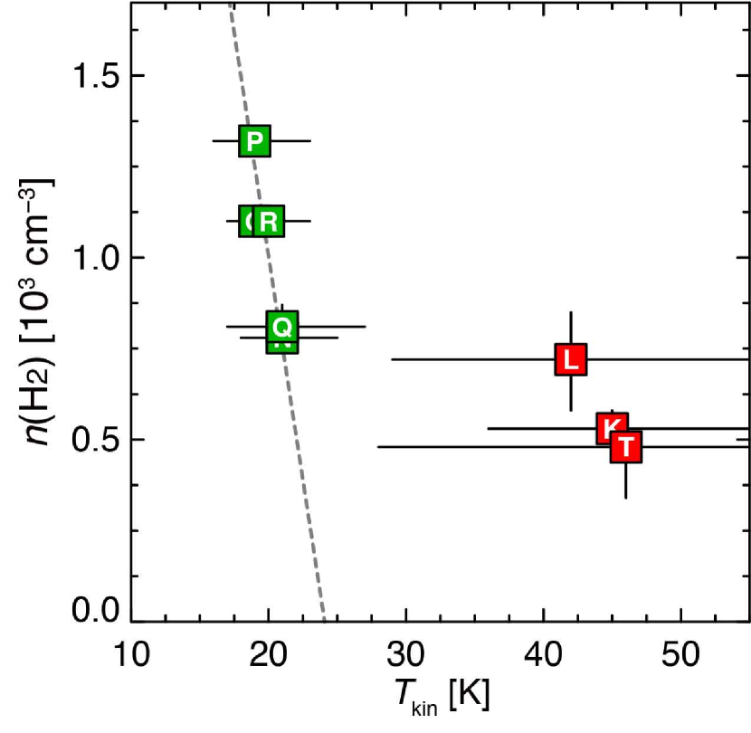
Figure 4: Scatter plot between $T_{\mathrm{kin}}$ and $n$(H₂). The dashed line indicates the linear regression using the least-squares method except for the CO clouds L, K, and T (see the text).

Figure 2 shows the typical LVG results, $T_{\mathrm{kin}}$–$n$(H₂) relation, and CO spectra for clouds P, R, and L. The post-shocked cloud L on the shock front shows higher kinetic temperature $T_{\mathrm{kin}}$ $\sim$42 K and relatively lower H₂ number density $n$(H₂) $\sim$720 cm^-3, while the ambient cloud P away from the SNR shell shows lower $T_{\mathrm{kin}}$ $\sim$19 K and moderate $n$(H₂) $\sim$1320 cm^-3. The pre-shocked cloud R lying between them shows similar values of $T_{\mathrm{kin}}$ and $n$(H₂) to the ambient cloud P ($T_{\mathrm{kin}}$ $\sim$20 K and $n$(H₂) $\sim$1100 cm^-3). This trend is also found in other molecular clouds in N49. It is noteworthy that clouds K, L, and T show lower ¹³CO($J$ = 2–1) / ¹²CO($J$ = 3–2) ratios than other clouds.

Figure 3 shows the radial distributions of X-ray intensity and $T_{\mathrm{kin}}$ of the eight molecular clouds from the geometric center of the SNR at ($\alpha_{\mathrm{J2000}}$, $\delta_{\mathrm{J2000}})=(05^{\mathrm{h}}25^{\mathrm{m}}59\fs 57$, $-66\arcdeg 04\arcmin 56\fs 4$). To calculate the shell diameter and thickness of the X-ray shell in N49, we performed a least-squares fitting using a three-dimensional spherical shell model with a Gaussian function $F(r)$ (e.g., Sano et al., 2017b, 2021a; Aruga et al., 2022):

$$F(r)=A\exp[-(r-r_{0}\bigr{)}^{2}/2\sigma^{2}],$$ (1)

where $A$ is the normalization factor of the Gaussian function, $r_{0}$ is the shell radius, $r$ is the radial distance from the geometric center of the SNR, and $\sigma$ is the standard deviation of the Gaussian function. We obtained a shell radius of $7.7\pm 1.8$ pc and shell thickness of $2.6\pm 4.5$ pc as the best-fit parameters of the fitting, where the shell thickness was defined as the FWHM of the Gaussian function.

Figure 4 shows the scatter plot between $T_{\mathrm{kin}}$ and $n$(H₂) for the eight molecular clouds. Clouds N, O, P, Q, and R show a negative correlation which was fitted by the least-squares method using the MPFITEXY routine (Williams et al., 2010), while $T_{\mathrm{kin}}$ of clouds K, L, and T seems to be shifted to higher values compared to the other molecular clouds.

4 Discussion

The observed spatial variation in $T_{\mathrm{kin}}$ and $n$(H₂) of the molecular clouds associated with N49 has many implications for the evolution of the supernova-shocked ISM. First, we argue that the high temperatures of $\sim$40–50 K as seen in clouds K, L, and T are likely caused by shock-heating. According to Paper I, these clouds are tightly interacting with shockwaves and enhance the turbulent magnetic field with bright synchrotron radiation on the surface of the shocked clouds, suggesting that clouds K, L, and T are located inside the SNR or on the shock front. Quantifying this scenario requires a decomposition of the density and velocity distribution of clouds K, L and T which requires even higher-resolution data (e.g., Menon et al., 2021; Sharda et al., 2022). Although clouds O, Q, and R have smaller radial distances than cloud K, this is likely due to projection effects. In addition, the observed cloud temperatures are roughly consistent with those measured in shock-heated molecular clouds associated with several Galactic SNRs (e.g., Seta et al., 1998; Sano et al., 2021a, b). The lack of local excitation sources other than SNR shocks also supports this scenario. If so, this is the first compelling evidence of “shock-heated” molecular clouds associated with an extragalactic SNR.

The shock-heating scenario is also consistent with the thermal conduction origin of the recombining plasma (RP) discovered in N49 (Uchida et al., 2015). The RP is characterized by a higher ionization temperature compared to the electron temperature, which is not expected in the classical evolution model of thermal plasma in SNRs (see also the review by Yamaguchi, 2020). To achieve the RP state, rapid electron cooling or an increase of the ionization state is needed. One of the possible scenarios is the rapid cooling of electrons via thermal conduction between the shocks and cold/dense clouds (e.g., Kawasaki et al., 2002; Matsumura et al., 2017a, b; Okon et al., 2018, 2020; Sano et al., 2021b). Paper I found that the hard-band X-rays due to radiative recombination are enhanced around the shocked clouds including clouds K, L, and T. The authors concluded that the RP in N49 was efficiently produced by shocked CO clouds due to thermal conduction, which is consistent with the higher kinetic temperatures of clouds K, L, and T. Additional spatially resolved X-ray spectroscopy with high-angular/spectral resolution is needed to confirm this scenario. The Athena mission has the potential to accomplish these (e.g., Nandra et al., 2013). It is noteworthy that the moderate dust temperature in cold components $\sim$20–30 K (pre-shocked dust) and in warm components $\sim$60 K (post-shocked dust) in N49 is also roughly consistent with our CO results (e.g., Otsuka et al., 2010; van Loon et al., 2010a; Lakićević et al., 2015), but the detailed comparison between the dust and CO clouds is beyond the scope of this paper.

Next, we argue that the moderate kinetic temperatures of $\sim$20 K seen in the other clouds N, O, P, Q, and R are likely due to cosmic-ray heating. According to Gabici et al. (2009), the diffusion length of cosmic rays $l_{\mathrm{diff}}$ in units of centimeters can be described as

$$l_{\mathrm{diff}}=\sqrt{4D(E,B)t_{\mathrm{age}}}\;,$$ (2)

where $D(E,B)$ is the diffusion coefficient in units of cm² s^-1 and $t_{\mathrm{age}}$ is the SNR age in units of seconds. $D(E,B)$ can be written using the accelerated cosmic-ray energy $E$ and the magnetic field strength $B$ as

$$D(E,B)=5\times 10^{26}\left(\frac{E}{100~{}\mathrm{MeV}}\right)^{0.5}\left(\frac{B}{10~{}\mathrm{\mu G}}\right)^{-0.5}\mathrm{}.\;\;\;$$ (3)

Adopting $t_{\mathrm{age}}=1.5\times 10^{11}$ s ($\sim$4800 yr; Park et al., 2012), $E=100$ MeV, and $B=10~{}\mu$G, we obtain $l_{\mathrm{diff}}\sim$6 pc which is substantially larger than the maximum separation between cloud P and the shock boundary of the SNR. This indicates that almost all cosmic ray particles accelerated in N49 have reached the entire region of the associated molecular clouds, and hence the cosmic-ray heating works equally well for both the post-shocked and pre-shocked clouds as well as the ambient clouds. In other words, cosmic-ray heating is not sufficient to increase the kinetic temperature of K, L, and T significantly above those of the unshocked clouds (O, Q, R, etc).

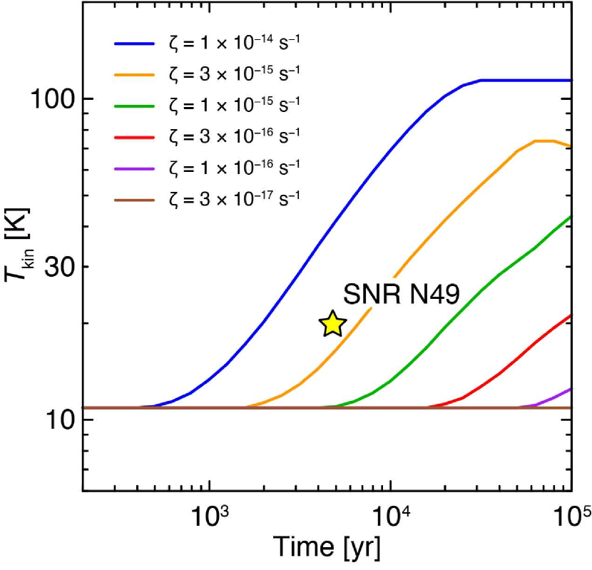
Figure 5: Time evolution of kinematic temperature $T_{\mathrm{kin}}$ at the cloud center after the supernova event that generates SNR N49. Colors indicate the assumed cosmic-ray ionization rate $\zeta$ from $3\times 10^{-17}$ s^-1 to $1\times 10^{-14}$ s^-1. The star symbol indicates the observed values of $T_{\mathrm{kin}}$ for the ambient or pre-shocked clouds at the age of N49 (4800 yr).

We also argue that the moderate temperatures of the cosmic-ray-irradiated clouds are naturally explained by the high cosmic-ray ionization rates surrounding the SNR. Figure 5 shows the time evolution of the kinematic temperature $T_{\mathrm{kin}}$ at the cloud center after the supernova event that generated the LMC SNR N49, which was calculated as a function of cosmic-ray ionization rates $\zeta$ using a photodissociation region (PDR) model (Furuya et al., 2022, see the Appendix for further details). Since the typical cosmic-ray ionization rates in the vicinity of Galactic SNRs are $\sim$30–300 times higher than the standard Galactic value of $\sim$$10^{-17}$ s^-1 (e.g., Indriolo et al., 2010; Ceccarelli et al., 2011; Vaupré et al., 2014), the observed values of $T_{\mathrm{kin}}$ $\sim$20 K at pre-shocked and ambient clouds can be explained as the cosmic-ray heating effect. Further follow-up observations using multiple emission lines such as HCO⁺, DCO⁺ (e.g., Vaupré et al., 2014), and/or [Ci] (Yamagishi et al., 2023) are needed to estimate the cosmic-ray ionization rate in the vicinity of the LMC SNR N49.

Another interesting point is that these clouds, when exposed to a large number of cosmic rays, likely emit gamma-rays and X-ray line emission. Recent Fermi-LAT analysis of N49 presented a possible detection of hadronic gamma-rays which were produced by proton–proton interactions (Campana et al., 2022). The Fe K$\alpha$ line emission at 6.4 keV was also discovered in several Galactic/Magellanic SNRs, which was probably produced by interactions between low-energy cosmic-ray protons and neutral irons in the ISM clouds (e.g., Nobukawa et al., 2018, 2019; Bamba et al., 2009, 2018; Okon et al., 2018). Further gamma-ray and X-ray observations at the high spatial and spectral resolutions using the Cherenkov Telescope Array (Actis et al., 2011; Cherenkov Telescope Array Consortium et al., 2019), the XRISM mission (Tashiro et al., 2020), and the Athena mission (Nandra et al., 2013) will allow us to unveil the high-energy radiation processes in N49.

Finally, we focus on possible cloud evaporation and/or destruction via shock-cloud interactions. In general, it is often assumed that interstellar gaseous clouds are immediately evaporated by supernova shocks in SNRs (e.g., Slavin et al., 2017; Wang et al., 2018; Zhang et al., 2019). However, this is correct only if the gas density contrast between the cloud and the inter-cloud gas densities is small, typically $\sim$100 or less. The initial ISM conditions before a core-collapse supernova explosion are expected to have a large density fluctuation of $\sim$10⁵ due to strong stellar winds from a massive progenitor. The low-density inter-cloud medium, such as atomic Hi gas, was completely swept up by the winds over $\sim$$10^{6}$ yr and then created a wind bubble with an interior density of $\sim$0.01 cm^-3 (Weaver et al., 1977). On the other hand, molecular clouds can survive wind erosion owing to their high densities, greater than $\sim$$10^{3}$ cm^-3. When the shocks encounter the molecular cloud, the shock velocity $V_{\mathrm{sh}}$ dramatically decelerates to $V_{\mathrm{sh}}/(n_{\mathrm{cloud}}/n_{0})^{0.5}$, where $n_{\mathrm{cloud}}$ is the cloud density and $n_{0}$ is the inter-cloud (ambient) density (see Section 39.3 in Draine, 2011). Adopting the density contrast $n_{\mathrm{cloud}}/n_{0}=10^{5}$, $V_{\mathrm{sh}}=3000$ km s^-1, and a cloud radius of 1 pc, the cloud-crossing time of supernova shocks is $\sim$$10^{5}$ yr, and hence the cloud can survive the shock destruction within the typical lifetime of a SNR (see also a review by Sano & Fukui, 2021).

We argue that the scenario can be applied to the SNR N49. The wind-bubble explosion scenario is consistent with the core-collapse origin of N49 (Gaensler et al., 2001; Klose et al., 2004; Badenes et al., 2009; Yamaguchi et al., 2014). The shocked molecular clouds are thought to have survived the erosion because we detect them using CO emission lines. Moreover, the negative correlation between $T_{\mathrm{kin}}$ and $n$(H₂) indicates that clouds N, O, P, Q, and R have constant pressure and thus did not undergo shock evaporation. The enhanced magnetic field via shock-cloud interactions may also suppress thermal conduction and hamper cloud evaporation (e.g., Orlando et al., 2008). Interestingly, clouds K, L, and T located inside or on the edge of the SNR shell are significantly shifted from this pressure-constant line to a higher-pressure region and have slightly reduced number densities $n$(H₂). This trend suggests that the clouds completely engulfed by shocks were partially evaporated through shock-cloud interactions. A similar trend is also seen in the shock-engulfed star-forming dense core C embedded within the Galactic SNR RX J1713.7$-$3946. Sano et al. (2010) presented a slightly steeper density gradient than the typical star-forming cloud core, suggesting that only the surface of the cloud has been stripped out and heated up. In any case, the molecular clouds engulfed by the fast shocks in N49 were shown to decrease in number density rather than increase.

5 Summary

We summarize our conclusions as follows.

1. New ¹²CO($J$ = 3–2, 2–1) and ¹³CO($J$ = 2–1) observations using ALMA have revealed clumpy distributions of molecular clouds associated with SNR N49 in the LMC at a resolution of $1\farcs 73\times 1\farcs 10$ or $\sim$0.3 pc. The clouds completely delineate the southeastern edge of the SNR shell and show a high-intensity ratio of ¹²CO($J$ = 2–1)/¹²CO($J$ = 1–0) $\sim$1.0–1.2, suggesting that shock-cloud interactions have occurred.

2. We applied a non-LTE LVG analysis toward the eight molecular clouds that are detected in ¹³CO($J$ = 2–1) emission with $3\sigma$ or higher significance. The kinetic temperature $T_{\mathrm{kin}}$ and number density of molecular hydrogen $n$(H₂) of the post-shocked clouds located inside or on the shock front differed significantly from the other pre-shocked or ambient clouds; the cloud near the shock front shows the highest $T_{\mathrm{kin}}$ $\sim$50 K and the lowest $n$(H₂) $\sim$0.5–$0.7\times 10^{3}$ cm^-3, while the cloud $\sim$5 pc away from the edge of the SNR has the lowest $T_{\mathrm{kin}}$ $\sim$20 K and the densest $n$(H₂) $\sim$$1.3\times 10^{3}$ cm^-3. Since the spatial variation of $T_{\mathrm{kin}}$ cannot be explained by cosmic-ray heating alone or extra heating sources like O-type stars, we conclude that the high $T_{\mathrm{kin}}$ values of the clouds were caused by supernova shocks. This is the first compelling evidence of shock-heated molecular clouds in an extragalactic SNR.

3. The negative correlation between $T_{\mathrm{kin}}$ and $n$(H₂) indicates that clouds N, O, P, Q, and R have constant pressure and did not experience shock evaporation within the short SNR age of $\sim$4800 yr. On the other hand, clouds K, L, and T, which are on the inside or on the edge of the shell, are significantly shifted from this pressure-constant line to a higher-pressure region and have slightly reduced densities, suggesting that the shock-engulfed clouds were partially evaporated through the shock-cloud interaction. The decreased density and increased pressure (and kinetic temperature) of the shocked molecular clouds have important implications for understanding the negative feedback of energetic supernova shocks on star formation. Further follow-up studies are needed from both the observational and theoretical sides.

APPENDIX
Time evolution of the kinetic temperature

To estimate the impact of the cosmic-ray heating on the kinetic temperature, we run one-dimensional plane parallel PDR models (Furuya et al., 2022), which solve the time evolution of the gas temperature and abundances of chemical species self-consistently for given gas density distribution and dust-temperature distribution, considering gas-phase and gas-grain interaction (i.e., adsorption and desorption) and heating and cooling processes. Elemental abundances are taken from Acharyya & Herbst (2015) (low metal abundances for the LMC in their Table 1). At the initial chemical state, we assume all hydrogen is in H₂, all carbon is in CO, and the remaining oxygen is in H₂O ice. The other elements are assumed to exist as either atoms or atomic ions in the gas phase.

The model simulation consists of two steps. In the first step, the model simulates the temporal evolution of the gas temperature and chemical abundances for 10⁷ yr, assuming the standard $\zeta$ value of $1\times 10^{-17}$ s^-1. The chosen timescale of 10⁷ yr is arbitrary, but it is long enough for the C⁺, C⁰, and CO abundances to reach steady-state values. In the second step, the model follows the evolution for $1\times 10^{5}$ yrs with an enhanced $\zeta$ value in a range between $3\times 10^{-17}$ s^-1 and $1\times 10^{-14}$ s^-1. The first and second steps mimic conditions just before and after the supernova explosion, respectively. As input parameters for the model, we employ the UV intensity $G_{0}$ = $110$ (Seok et al., 2012) and the hydrogen (Hi+H₂) gas density $n_{\mathrm{HI+H_{2}}}$ = $1\times 10^{3}$ cm^-3. The dust temperature is calculated as a function of $A_{V}$ using Equation 8 in Hocuk et al. (2017). The ratio of the hydrogen column density to $A_{V}$ is assumed to be $3.5\times 10^{21}$ cm^-2 (Cox et al., 2006). The gas temperature evolution at the cloud center ($A_{V}=5$ mag.) after the explosion is shown in Figure 5.

References

- Acharyya & Herbst (2015) Acharyya, K., & Herbst, E. 2015, ApJ, 812, 142, doi: 10.1088/0004-637X/812/2/142
- Actis et al. (2011) Actis, M., Agnetta, G., Aharonian, F., et al. 2011, Experimental Astronomy, 32, 193, doi: 10.1007/s10686-011-9247-0
- Anderl et al. (2014) Anderl, S., Gusdorf, A., & Güsten, R. 2014, A&A, 569, A81, doi: 10.1051/0004-6361/201423561
- Aruga et al. (2022) Aruga, M., Sano, H., Fukui, Y., et al. 2022, ApJ, 938, 94, doi: 10.3847/1538-4357/ac90c6
- Badenes et al. (2009) Badenes, C., Harris, J., Zaritsky, D., & Prieto, J. L. 2009, ApJ, 700, 727, doi: 10.1088/0004-637X/700/1/727
- Bamba et al. (2009) Bamba, A., Yamazaki, R., Kohri, K., et al. 2009, ApJ, 691, 1854, doi: 10.1088/0004-637X/691/2/1854
- Bamba et al. (2018) Bamba, A., Ohira, Y., Yamazaki, R., et al. 2018, ApJ, 854, 71, doi: 10.3847/1538-4357/aaa5a0
- Banas et al. (1997) Banas, K. R., Hughes, J. P., Bronfman, L., & Nyman, L. Å. 1997, ApJ, 480, 607, doi: 10.1086/303989
- Blake et al. (1987) Blake, G. A., Sutton, E. C., Masson, C. R., & Phillips, T. G. 1987, ApJ, 315, 621, doi: 10.1086/165165
- Bozzetto et al. (2017) Bozzetto, L. M., Filipović, M. D., Vukotić, B., et al. 2017, ApJS, 230, 2, doi: 10.3847/1538-4365/aa653c
- Campana et al. (2022) Campana, R., Massaro, E., Bocchino, F., et al. 2022, MNRAS, 515, 1676, doi: 10.1093/mnras/stac1875
- CASA Team et al. (2022) CASA Team, Bean, B., Bhatnagar, S., et al. 2022, PASP, 134, 114501, doi: 10.1088/1538-3873/ac9642
- Ceccarelli et al. (2011) Ceccarelli, C., Hily-Blant, P., Montmerle, T., et al. 2011, ApJ, 740, L4, doi: 10.1088/2041-8205/740/1/L4
- Cherenkov Telescope Array Consortium et al. (2019) Cherenkov Telescope Array Consortium, Acharya, B. S., Agudo, I., et al. 2019, Science with the Cherenkov Telescope Array (World Scientific), doi: 10.1142/10986
- Cornett et al. (1977) Cornett, R. H., Chin, G., & Knapp, G. R. 1977, A&A, 54, 889
- Cornwell (2008) Cornwell, T. J. 2008, IEEE Journal of Selected Topics in Signal Processing, 2, 793, doi: 10.1109/JSTSP.2008.2006388
- Cox et al. (2006) Cox, N. L. J., Cordiner, M. A., Cami, J., et al. 2006, A&A, 447, 991, doi: 10.1051/0004-6361:20053367
- Draine (2011) Draine, B. T. 2011, Physics of the Interstellar and Intergalactic Medium (Princeton Univ. Press)
- Fruscione et al. (2006) Fruscione, A., McDowell, J. C., Allen, G. E., et al. 2006, in Society of Photo-Optical Instrumentation Engineers (SPIE) Conference Series, Vol. 6270, Society of Photo-Optical Instrumentation Engineers (SPIE) Conference Series, ed. D. R. Silva & R. E. Doxsey, 62701V, doi: 10.1117/12.671760
- Fujii et al. (2014) Fujii, K., Minamidani, T., Mizuno, N., et al. 2014, ApJ, 796, 123, doi: 10.1088/0004-637X/796/2/123
- Fukui et al. (2019) Fukui, Y., Tokuda, K., Saigo, K., et al. 2019, ApJ, 886, 14, doi: 10.3847/1538-4357/ab4900
- Furuya et al. (2022) Furuya, K., Tsukagoshi, T., Qi, C., et al. 2022, ApJ, 926, 148, doi: 10.3847/1538-4357/ac45ff
- Gabici et al. (2009) Gabici, S., Aharonian, F. A., & Casanova, S. 2009, MNRAS, 396, 1629, doi: 10.1111/j.1365-2966.2009.14832.x
- Gaensler et al. (2001) Gaensler, B. M., Slane, P. O., Gotthelf, E. V., & Vasisht, G. 2001, ApJ, 559, 963, doi: 10.1086/322358
- Goldreich & Kwan (1974) Goldreich, P., & Kwan, J. 1974, ApJ, 189, 441, doi: 10.1086/152821
- Graessle et al. (2007) Graessle, D. E., Evans, I. N., Glotfelty, K., et al. 2007, Chandra News, 14, 33
- Hocuk et al. (2017) Hocuk, S., Szűcs, L., Caselli, P., et al. 2017, A&A, 604, A58, doi: 10.1051/0004-6361/201629944
- Hogge et al. (2019) Hogge, T. G., Jackson, J. M., Allingham, D., et al. 2019, ApJ, 887, 79, doi: 10.3847/1538-4357/ab5180
- Indriolo et al. (2010) Indriolo, N., Blake, G. A., Goto, M., et al. 2010, ApJ, 724, 1357, doi: 10.1088/0004-637X/724/2/1357
- Inoue et al. (2009) Inoue, T., Yamazaki, R., & Inutsuka, S.-i. 2009, ApJ, 695, 825, doi: 10.1088/0004-637X/695/2/825
- Inoue et al. (2012) Inoue, T., Yamazaki, R., Inutsuka, S.-i., & Fukui, Y. 2012, ApJ, 744, 71, doi: 10.1088/0004-637X/744/1/71
- Inutsuka et al. (2015) Inutsuka, S.-i., Inoue, T., Iwasaki, K., & Hosokawa, T. 2015, A&A, 580, A49, doi: 10.1051/0004-6361/201425584
- Kawasaki et al. (2002) Kawasaki, M. T., Ozaki, M., Nagase, F., et al. 2002, ApJ, 572, 897, doi: 10.1086/340383
- Klose et al. (2004) Klose, S., Henden, A. A., Geppert, U., et al. 2004, ApJ, 609, L13, doi: 10.1086/422657
- Körtgen et al. (2016) Körtgen, B., Seifried, D., Banerjee, R., Vázquez-Semadeni, E., & Zamora-Avilés, M. 2016, MNRAS, 459, 3460, doi: 10.1093/mnras/stw824
- Lakićević et al. (2015) Lakićević, M., van Loon, J. T., Meixner, M., et al. 2015, ApJ, 799, 50, doi: 10.1088/0004-637X/799/1/50
- Landsman (1993) Landsman, W. B. 1993, in Astronomical Society of the Pacific Conference Series, Vol. 52, Astronomical Data Analysis Software and Systems II, ed. R. J. Hanisch, R. J. V. Brissenden, & J. Barnes, 246
- Matsumura et al. (2017a) Matsumura, H., Tanaka, T., Uchida, H., Okon, H., & Tsuru, T. G. 2017a, ApJ, 851, 73, doi: 10.3847/1538-4357/aa9bdf
- Matsumura et al. (2017b) Matsumura, H., Uchida, H., Tanaka, T., et al. 2017b, PASJ, 69, 30, doi: 10.1093/pasj/psx001
- Mazumdar et al. (2022) Mazumdar, P., Tram, L. N., Wyrowski, F., Menten, K. M., & Tang, X. 2022, A&A, 668, A180, doi: 10.1051/0004-6361/202037564
- Menon et al. (2021) Menon, S. H., Federrath, C., Klaassen, P., Kuiper, R., & Reiter, M. 2021, MNRAS, 500, 1721, doi: 10.1093/mnras/staa3271
- Minamidani et al. (2011) Minamidani, T., Tanaka, T., Mizuno, Y., et al. 2011, AJ, 141, 73, doi: 10.1088/0004-6256/141/3/73
- Mizuno et al. (2010) Mizuno, Y., Kawamura, A., Onishi, T., et al. 2010, PASJ, 62, 51, doi: 10.1093/pasj/62.1.51
- Nandra et al. (2013) Nandra, K., Barret, D., Barcons, X., et al. 2013, arXiv e-prints, arXiv:1306.2307, doi: 10.48550/arXiv.1306.2307
- Nobukawa et al. (2019) Nobukawa, K. K., Hirayama, A., Shimaguchi, A., et al. 2019, PASJ, 71, 115, doi: 10.1093/pasj/psz099
- Nobukawa et al. (2018) Nobukawa, K. K., Nobukawa, M., Koyama, K., et al. 2018, ApJ, 854, 87, doi: 10.3847/1538-4357/aaa8dc
- Okon et al. (2018) Okon, H., Uchida, H., Tanaka, T., Matsumura, H., & Tsuru, T. G. 2018, PASJ, 70, 35, doi: 10.1093/pasj/psy022
- Okon et al. (2020) Okon, H., Tanaka, T., Uchida, H., et al. 2020, ApJ, 890, 62, doi: 10.3847/1538-4357/ab6987
- Orlando et al. (2008) Orlando, S., Bocchino, F., Reale, F., Peres, G., & Pagano, P. 2008, ApJ, 678, 274, doi: 10.1086/529420
- Otsuka et al. (2010) Otsuka, M., van Loon, J. T., Long, K. S., et al. 2010, A&A, 518, L139, doi: 10.1051/0004-6361/201014642
- Park et al. (2020) Park, S., Bhalerao, J., Kargaltsev, O., & Slane, P. O. 2020, ApJ, 894, 17, doi: 10.3847/1538-4357/ab83f8
- Park et al. (2003) Park, S., Burrows, D. N., Garmire, G. P., et al. 2003, ApJ, 586, 210, doi: 10.1086/367619
- Park et al. (2012) Park, S., Hughes, J. P., Slane, P. O., et al. 2012, ApJ, 748, 117, doi: 10.1088/0004-637X/748/2/117
- Pietrzyński et al. (2013) Pietrzyński, G., Graczyk, D., Gieren, W., et al. 2013, Nature, 495, 76, doi: 10.1038/nature11878
- Reach & Rho (1999) Reach, W. T., & Rho, J. 1999, ApJ, 511, 836, doi: 10.1086/306703
- Rho et al. (2017) Rho, J., Hewitt, J. W., Bieging, J., et al. 2017, ApJ, 834, 12, doi: 10.3847/1538-4357/834/1/12
- Rho et al. (2015) Rho, J., Hewitt, J. W., Boogert, A., Kaufman, M., & Gusdorf, A. 2015, ApJ, 812, 44, doi: 10.1088/0004-637X/812/1/44
- Rho & Petre (1998) Rho, J., & Petre, R. 1998, ApJ, 503, L167, doi: 10.1086/311538
- Sano & Fukui (2021) Sano, H., & Fukui, Y. 2021, Ap&SS, 366, 58, doi: 10.1007/s10509-021-03960-4
- Sano et al. (2021a) Sano, H., Suzuki, H., Nobukawa, K. K., et al. 2021a, ApJ, 923, 15, doi: 10.3847/1538-4357/ac1c02
- Sano et al. (2010) Sano, H., Sato, J., Horachi, H., et al. 2010, ApJ, 724, 59, doi: 10.1088/0004-637X/724/1/59
- Sano et al. (2017a) Sano, H., Fujii, K., Yamane, Y., et al. 2017a, in American Institute of Physics Conference Series, Vol. 1792, 6th International Symposium on High Energy Gamma-Ray Astronomy, 040038, doi: 10.1063/1.4968942
- Sano et al. (2017b) Sano, H., Yamane, Y., Voisin, F., et al. 2017b, ApJ, 843, 61, doi: 10.3847/1538-4357/aa73e0
- Sano et al. (2021b) Sano, H., Yoshiike, S., Yamane, Y., et al. 2021b, ApJ, 919, 123, doi: 10.3847/1538-4357/ac0dba
- Sault et al. (1995) Sault, R. J., Teuben, P. J., & Wright, M. C. H. 1995, in Astronomical Society of the Pacific Conference Series, Vol. 77, Astronomical Data Analysis Software and Systems IV, ed. R. A. Shaw, H. E. Payne, & J. J. E. Hayes, 433, doi: 10.48550/arXiv.astro-ph/0612759
- Scoville & Solomon (1974) Scoville, N. Z., & Solomon, P. M. 1974, ApJ, 187, L67, doi: 10.1086/181398
- Seok et al. (2012) Seok, J. Y., Koo, B.-C., & Onaka, T. 2012, ApJ, 744, 160, doi: 10.1088/0004-637X/744/2/160
- Seta et al. (1998) Seta, M., Hasegawa, T., Dame, T. M., et al. 1998, ApJ, 505, 286, doi: 10.1086/306141
- Sharda et al. (2022) Sharda, P., Menon, S. H., Federrath, C., et al. 2022, MNRAS, 509, 2180, doi: 10.1093/mnras/stab3048
- Slavin et al. (2017) Slavin, J. D., Smith, R. K., Foster, A., et al. 2017, ApJ, 846, 77, doi: 10.3847/1538-4357/aa8552
- Subramanian & Subramaniam (2010) Subramanian, S., & Subramaniam, A. 2010, A&A, 520, A24, doi: 10.1051/0004-6361/201014201
- Tashiro et al. (2020) Tashiro, M., Maejima, H., Toda, K., et al. 2020, in Society of Photo-Optical Instrumentation Engineers (SPIE) Conference Series, Vol. 11444, Space Telescopes and Instrumentation 2020: Ultraviolet to Gamma Ray, ed. J.-W. A. den Herder, S. Nikzad, & K. Nakazawa, 1144422, doi: 10.1117/12.2565812
- Tokuda et al. (2019) Tokuda, K., Fukui, Y., Harada, R., et al. 2019, ApJ, 886, 15, doi: 10.3847/1538-4357/ab48ff
- Uchida et al. (2015) Uchida, H., Koyama, K., & Yamaguchi, H. 2015, ApJ, 808, 77, doi: 10.1088/0004-637X/808/1/77
- van Loon et al. (2010a) van Loon, J. T., Oliveira, J. M., Gordon, K. D., Sloan, G. C., & Engelbracht, C. W. 2010a, AJ, 139, 1553, doi: 10.1088/0004-6256/139/4/1553
- van Loon et al. (2010b) van Loon, J. T., Oliveira, J. M., Gordon, K. D., et al. 2010b, AJ, 139, 68, doi: 10.1088/0004-6256/139/1/68
- Vaupré et al. (2014) Vaupré, S., Hily-Blant, P., Ceccarelli, C., et al. 2014, A&A, 568, A50, doi: 10.1051/0004-6361/201424036
- Wang et al. (2018) Wang, Y., Bao, B., Yang, C., & Zhang, L. 2018, MNRAS, 478, 2948, doi: 10.1093/mnras/sty1275
- Weaver et al. (1977) Weaver, R., McCray, R., Castor, J., Shapiro, P., & Moore, R. 1977, ApJ, 218, 377, doi: 10.1086/155692
- White et al. (1987) White, G. J., Rainey, R., Hayashi, S. S., & Kaifu, N. 1987, A&A, 173, 337
- Williams et al. (2010) Williams, M. J., Bureau, M., & Cappellari, M. 2010, MNRAS, 409, 1330, doi: 10.1111/j.1365-2966.2010.17406.x
- Wong et al. (2019) Wong, T., Hughes, A., Tokuda, K., et al. 2019, ApJ, 885, 50, doi: 10.3847/1538-4357/ab46ba
- Yamagishi et al. (2023) Yamagishi, M., Furuya, K., Sano, H., et al. 2023, arXiv e-prints, arXiv:2306.15983, doi: 10.48550/arXiv.2306.15983
- Yamaguchi (2020) Yamaguchi, H. 2020, Astronomische Nachrichten, 341, 150, doi: 10.1002/asna.202023771
- Yamaguchi et al. (2014) Yamaguchi, H., Badenes, C., Petre, R., et al. 2014, ApJ, 785, L27, doi: 10.1088/2041-8205/785/2/L27
- Yamane et al. (2018) Yamane, Y., Sano, H., van Loon, J. T., et al. 2018, ApJ, 863, 55, doi: 10.3847/1538-4357/aacfff
- Zhang et al. (2019) Zhang, G.-Y., Slavin, J. D., Foster, A., et al. 2019, ApJ, 875, 81, doi: 10.3847/1538-4357/ab0f9a
- Zhou et al. (2019) Zhou, P., Vink, J., Safi-Harb, S., & Miceli, M. 2019, A&A, 629, A51, doi: 10.1051/0004-6361/201936002
- Zhou et al. (2022) Zhou, P., Zhang, G.-Y., Zhou, X., et al. 2022, ApJ, 931, 144, doi: 10.3847/1538-4357/ac63b5