The DECam Ecliptic Exploration Project (DEEP) II. Observational Strategy and Design

Abstract

We present the DECam Ecliptic Exploration Project (DEEP) survey strategy including observing cadence for orbit determination, exposure times, field pointings and filter choices. The overall goal of the survey is to discover and characterize the orbits of a few thousand Trans-Neptunian Objects (TNOs) using the Dark Energy Camera (DECam) on the Cerro Tololo Inter-American Observatory (CTIO) Blanco 4 meter telescope. The experiment is designed to collect a very deep series of exposures totaling a few hours on sky for each of several 2.7 square degree DECam fields-of-view to achieve magnitude $\sim 26.2$ using a wide $V\!R$ filter which encompasses both the $V$ and $R$ bandpasses. In the first year, several nights were combined to achieve a sky area of about 34 square degrees. In subsequent years, the fields have been re-visited to allow TNOs to be tracked for orbit determination. When complete, DEEP will be the largest survey of the outer solar system ever undertaken in terms of newly discovered object numbers, and the most prolific at producing multi-year orbital information for the population of minor planets beyond Neptune at 30 au.

1 Introduction

For decades, the properties of the Kuiper Belt and Trans-Neptunian region have been, and still remain to this day, observationally limited. The only way to improve this situation is by discovering more objects and characterizing their orbital and physical properties. As of June 1, 2023, there are 2,429 multi-opposition Trans-Neptunian Objects (TNOs) listed by the Minor Planet Center. Survey completion rates for the brightest objects are higher than for other TNO populations, with perhaps $\gtrsim 75\%$ of the dwarf planet-sized objects known in the Northern hemisphere (Schwamb et al., 2014) and a similar efficiency in the Southern hemisphere (Sheppard et al., 2011; Rabinowitz et al., 2012) out to heliocentric distances of $\sim 100$ au. These large bodies have diameters $D\gtrsim 450$ km (Tancredi & Favre, 2008; Pinilla-Alonso et al., 2020) and typically are brighter than red magnitude $m_{R}\lesssim 20$ interior to heliocentric distances of $R\lesssim 40$ au. However, since there are far more smaller TNOs ($D\lesssim 100$ km, $m_{R}\gtrsim 23$) than large TNOs, the known sample of $D\sim 100$ km TNOs is a small fraction of the inferred population. Estimates of the small population vary, but recent ground-based surveys with hundred of detections find the number density of TNOs near the ecliptic at $m_{R}\simeq 24.5$ (about $D\lesssim 25$ km for albedos of 15%) to be more than 5 objects per square degree (Bannister et al., 2018) suggesting that there are tens of thousands of such bodies which remain undiscovered, a population size that has been refined, but not changed in overall magnitude in decades (Trujillo et al., 2001). It is clear that our knowledge of the number of TNOs is far from complete — likely more incomplete than any other stable solar system population except for the extremely distant Extreme Trans-Neptunian Objects (ETNOs) beyond 50 au (Sheppard et al., 2019).

It is this main deficiency of our knowledge of the TNOs that was the impetus for our project. The main science goals and how they impact our observational design are discussed in more detail in Section 2. Although these science goals have been previously studied by other surveys, none have done so in as great detail as in this survey. In the Dark Energy Camera (DECam) Ecliptic Exploration Project (DEEP), we expect to discover a few thousand new TNOs and trace their orbits over several years. In this work, we discuss the observational choices that were made to achieve this goal and to achieve the scientific goals of our project. Other works discuss the methods used to discover new bodies (Gerdes et al., 2022; Jurić et al., 2019) and investigations of other populations such as the main belt asteroids (Trilling et al., 2021).

We expect that our survey, when complete, will be an improvement on prior surveys in terms of discovery statistics by factors of a few. Prior works can largely be classified into three categories: (1) very wide-area ($>1,000$ square degrees) but shallow ($m_{R}<21$) surveys which are designed to maximize the discovery rate of dwarf planet sized objects (Trujillo & Brown, 2003; Schwamb et al., 2009, 2010; Sheppard et al., 2011; Rabinowitz et al., 2012), (2) moderately wide-area surveys ($\sim 100$ square degrees) investigating somewhat fainter magnitudes ($m_{R}\sim 24$) (Trujillo et al., 2001; Elliot et al., 2005; Petit et al., 2011; Bannister et al., 2018; Sheppard et al., 2019; Bernardinelli et al., 2020, 2022) and (3) very deep ($m_{R}>24.5$) but small-area surveys ($<50$ sq deg) probing the faintest TNOs (Gladman et al., 1998; Chiang & Brown, 1999; Bernstein et al., 2004; Parker & Kavelaars, 2010). It is beyond the scope of this work to summarize these (and many other) surveys — for a more comprehensive work on these surveys and many other aspects of the TNOs, see Prialnik et al. (2020).

One of our primary survey goals was to maximize total number of objects discovered with orbital information. This simple choice created several constraints on our survey in terms of optimization: (1) a survey duration of 1–3 years was required to understand TNO orbits, which tend to have orbital periods of order $\sim 200$ years for bodies at 50 au and nearer, (2) since the size distribution of the TNOs strongly favors faint bodies, a large telescope ($\gtrsim 4$ m) was needed to reach magnitudes of $m_{R}>24$, and (3) since total number of bodies was important, and the TNOs are known to have an ecliptic plane density of about 1 body per square degree for magnitude $m_{R}\sim 24$, our telescope needed to have a wide field of view given its size. With these parameters in mind, our instrument of choice was the DECam instrument mounted at prime focus on the Víctor M. Blanco 4 m telescope atop Cerro Tololo, Chile. These choices also affected our observing strategy, which was to maximize survey depth, meaning that we would observe for typically $\sim 4$ hours on sky for any given field.

The DECam instrument on the Blanco 4 m is an excellent instrument for this study due to its large field of view ($\sim 2.7$ square degrees) on a large telescope ($D\sim 4$ m) with $\sim 1\arcsec$ full-width-at-half-maximum seeing at a site relatively protected from light pollution, which compares well with other survey instruments in terms of lightgrasp (Trujillo, 2008). Our overall survey expectations (discussed in more detail in Section 3) are that we should be able to probe to limiting magnitude $m_{R}\sim 26.2$ over 32 – 108 square degrees over a few years, which will generate the discovery of a few thousand new TNOs and allow orbital properties to be constrained for many of them.

This total number of objects should significantly exceed prior works, which for any given work have discovered $<1,000$ total objects and in many cases far fewer. Our survey is complementary to the expected data characteristics to be produced by the Vera C. Rubin Observatory Legacy Survey of Space and Time (LSST). The LSST has an exposure time of about 30 s on a 6.7 m effective aperture telescope, resulting in a survey depth of about $m_{R}\sim 24.5$ (LSST Science Collaboration et al., 2009; Vera C. Rubin Observatory LSST Solar System Science Collaboration et al., 2021). Since it will survey the entire sky available from Cerro Pachón, which includes most of the ecliptic, it should find some $\sim 40,000$ TNOs brighter than $m_{R}\sim 24.5$. Although the total number of TNOs discovered by the LSST, which is a billion dollar project planned to span about a decade of operations, will far exceed our survey, our survey is deeper, $m_{R}\sim 26.2$, which corresponds to smaller objects ($\sim 2.5$ smaller diameter) and will be complete before the LSST begins full survey operations.

2 Guiding Principles of the Survey

To constrain our overall survey design, we adopted principles derived from our science goals. The main science goals are discussed in more detail by Trilling et al. (2019) but in summary are: (1) measure the size distribution of the TNOs down to 25 km, (2) measure the colors of about one thousand TNOs, (3) derive the shape distribution of TNOs from partial lightcurves, and (4) measure colors, size distribution, and shapes as a function of dynamical class and size.

Additional secondary science goals are related to other populations such as the main belt asteroids, Centaurs and Trojan asteroids.

The guiding principles derived from these science goals follow:

• Survey depth is more important than measuring color. That is because the survey’s main goal is to probe small sizes and discover large numbers of objects.

• Uniform depth per observing run per field is the most important feature of the survey. This will allow the ability to track objects consistently throughout the survey.

• Colors will only be measured after uniform depth is reached in the $V\!R$ filter. This is because of the prior two principles and also because if objects’ orbits are well-known, colors can be obtained in later epochs if need be.

• We want to observe each object twice in the first year, once near opposition and once a month from opposition. Each object will then be observed in years 2 and 3 as well. The inclusion of the off-opposition observation allows for a better orbit solution than purely opposition observations, with a factor 10 lower astrometric error after the survey is completed (see Figure 2).

• We will track objects over the multi-year course of the survey, so we must expand our sky coverage as objects with different orbits disperse from their initial Year 1 discovery locations (Figure 2).

• Objects in the outer solar system, beyond 30 au, are the primary goal, but science cases involving closer objects, including the main belt asteroids, will also be probed.

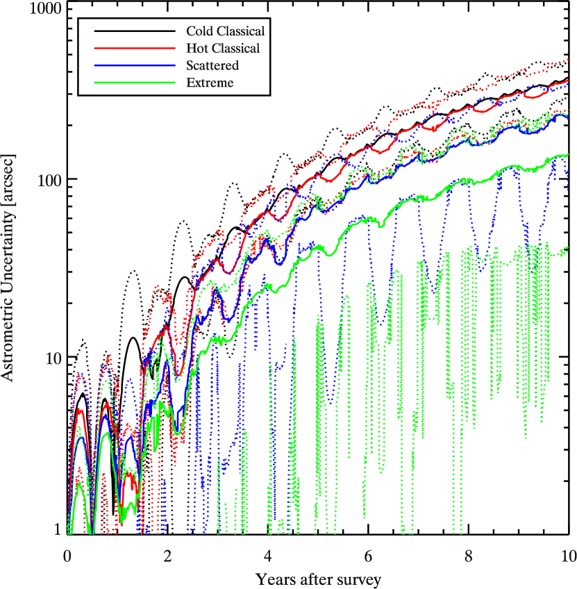
Figure 1: Astrometric uncertainty after our survey is completed for different classes of TNOs. Simulated orbits were used to create simulated observations with the addition of Gaussian noise of 0.6 arc-seconds in sky position similar to or greater than our actual astrometric uncertainty. Orbits were then fit to the simulated observations using the technique of Bernstein & Khushalani (2000). Object location predictions after survey completion were then compared to true simulated observations to determine astrometric uncertainty. Solid lines mark the median astrometric error while dashed lines bound the 90% confidence region for each orbit type. Most populations maintain $<30$ arc-second error a few years after survey completion.

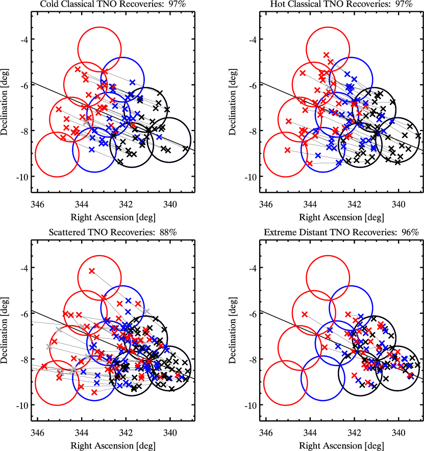
Figure 2: A visualization of our recovery efficiency is shown. Circles approximate the DECam field positions. Black fields (rightmost 3 fields) were imaged in Years 1–3, blue (center 3) in Years 2–3 and red (leftmost fields) in Year 3. Four populations of TNOs were modeled with simulated discovered objects shown as crosses with color coding for the year they are imaged. Grey crosses represent objects that are not imaged in a given year and grey lines connect object positions across epochs. Recovery efficiency is nearly 90% or more for all classes of objects. The numbers of plotted objects have been reduced for clarity to depict orbital motion. In reality many thousands of objects were simulated and are expected to be discovered in the survey. The black line represents the solar system invariable plane as defined by Souami & Souchay (2012a).

3 Observing Strategy

Following the guiding principles, our observing strategy is summarized here, including the selection of the instrumentation for the experiment, the exposure times, filter choices and field locations.

3.1 Instrumentation

The basic choice we made for the instrument was the prime focus DECam camera on the Blanco 4m telescope at Cerro Tololo. The telescope itself is historic, completed in 1976 as a southern counterpart to the Kitt Peak Mayall 4m telescope. With the recent upgrade of instrumentation at the Blanco 4m telescope to the Dark Energy Camera (DECam), the DECam/Blanco instrument combination became one of the leading survey instruments in the world (Abbott et al., 2018).

We were granted a large survey program using DECam to survey our region over a three year period. Given the amount of telescope time devoted to the survey, $\sim 50$ observation dates, most of which were half-nights, we expect that the findings of the survey will remain relevant for a decade or longer.

3.2 Exposure Times

Exposure times must be relatively short so that asteroids do not trail much given their apparent rate of motion and the typical image quality, one of our secondary science goals. Typical asteroid motion at heliocentric distances from 2 au to 3.5 au at opposition is 43 to 28 arc-seconds/hour (Jewitt et al., 1996). In the best seeing conditions for the DECam instrument, 0.8 arc-seconds, the fastest asteroids will not trail with exposure times of 0.8 arc-seconds / (43 arc-seconds / hour) x 3600 seconds / hour = 67 seconds. Readout time for DECam is about 20 s, so choosing such an exposure time would equate to an open shutter efficiency of 77% (0.14 magnitudes loss compared to 100%). The optimum exposure time is therefore a trade-off between limiting magnitude for the asteroids, which suggests shorter exposures, compared to open-shutter efficiency which affects the limiting magnitude for the slower objects, which suggests longer exposures.

To strike a balance between those two competing factors, we have chosen an exposure time of 120 seconds. This yields efficiency due to the readout time of 86% (0.08 magnitude loss for slow objects). In terms of trailing loss (applicable to the fastest objects) this would be 0.17 to 0 magnitudes trailing loss for slowest asteroids (28 arc-seconds per hour) in seeing of 0.8 arc-seconds to 1.1 arc-seconds. And this exposure time yields 0.6 to 0.3 magnitudes trailing loss for fastest asteroids (43 arc-seconds per hour) in similar seeing conditions.

3.3 Expected Survey Depth in $V\!R$ and Predicted Discovery Numbers

We can estimate the survey depth based on the performance achieved during the Dark Energy Survey (DES) DR1 (Abbott et al., 2018). The bandpass of our chosen filter, the $V\!R$ filter, is not specifically studied in Abbott et al. (2018), but is roughly equivalent in terms of total wavelength breadth and somewhat superior in overall throughput to that of $g$ and $r$ combined from the DES DR1 (see Section 3.4). The overall sensitivity of a single 90 second exposure in $g$ and $r$ was estimated to be $g=23.57$ and $r=23.34$ for signal-to-noise ratios of 10 ($S/N=10$) for the DES DR1. Since $S/N$ is proportional to the square root of exposure time $t$, and similarly the square root of overall bandpass $b_{p}$, as $S/N\sim\sqrt{b_{p}}$, we expect our limiting magnitude $m_{R}$ from filter change alone to be roughly $m_{r}\approx 0.5\times(23.34+23.57)+2.5\log(\sqrt{2})=23.83$.

In addition, we expect to take about $\sim 100$ images each of 120 seconds compared to the 90 second single images discussed in Abbott et al. (2018). Also, we only need $S/N=6.5$ for detection, as compared to the DES DR1 $S/N=10$. We expect that our combination of images will not be as efficient as the static sky DES found primarily because we are canvassing many possible apparent rates of objects in our analysis. Not only this, but since we plan to subtract a static image template, in some cases residual flux remains from slowly moving objects. The theoretical magnitude increase for the full DES survey, which targets about 10 images per sky location, would be $1.25\log(10)=1.25$ magnitudes. The actual realized performance appeared to be about 0.5 magnitudes less than this as the mean survey-wide magnitude limits for $g$ and $r$ are 24.33 and 24.08 respectively (for the co-add magnitude limit with 1.95 arc-seconds diameter, $S/N=10$), which are 0.76 and 0.74 magnitudes better than the single image depth, a loss of about 0.5 magnitude over the theoretical maximum. We expect our multiple-image depth to be worse than this since our objects are moving and are found by combining images assuming apparent rates for possible objects since we do not a priori know their apparent motion rates. Assuming that our image combination loss to be about 0.75 magnitudes versus the DES performance, we expect our limiting magnitude $m_{r}$ (which is roughly equivalent to $m_{R}$) to follow:

$$m_{R} \approx 23.83+1.25\log\frac{120\mbox{ s}}{90\mbox{ s}}+1.25\log\frac{100\mbox{ exposures}}{1\mbox{ exposure}}+2.5\log\frac{10}{6.5}-0.75\mbox{ image combination correction}$$

$$m_{R} \approx 26.21$$

This image depth of approximately $\sim 26.2$ is well beyond that expected for the LSST single image depth, as well as any other prior wide-field survey sensitive to TNOs.

Given the image depth of $\sim 26.2$, we can estimate how many objects we might we discover at that depth. To date, no surveys have observed this faint for this amount of sky area so this number is highly uncertain. For this estimate, we choose a comparison survey that is of similar depth since surveys that are not as sensitive suffer from extrapolation and surveys that are fainter tend to have lower number statistics. Perhaps the most relevant similar survey is that of Fuentes et al. (2009) who used data from the Subaru 8.2 m telescope to detect 82 TNOs to a depth of $R=25.7$ with a sky area of 3.57 square degrees near the ecliptic in a re-analysis of data collected for a Uranian satellite search (Sheppard et al., 2005). These results yield an ecliptic density of 23 objects per square degree. Since our survey is about 0.5 magnitude fainter, using the brightness distribution from Fuentes et al. (2009) with the slope of the faint object apparent magnitude distribution $\alpha=0.3$ derived from all surveys at the time, this magnitude difference would result in a correction factor of $10^{0.3\times 0.5}=1.41$ times more objects, yielding an expected ecliptic detection rate of 32 objects per square degree.

Using this number, we can extrapolate to our survey area. Here, we make the distinction between full-survey objects (that is, objects tracked throughout the entire survey and which have reliable orbital information) and partial-survey objects (which, in the final planned year would have distance and brightness information but uncertain orbits). For the former population, we imaged 4 patches of sky throughout the year for each of 3 fields. For the latter population, we imaged 4 patches of sky throughout the year for each of 10 fields. Since the DECam camera is about 2.7 square degrees, this is an effective sky area of between 32 and 108 square degrees. Thus, we expect to discover about 1,000 objects with well-determined orbits and 3,500 objects with enough information to measure apparent magnitude and radial distributions.

3.4 Optimal Filters for TNO Colors

In order to assess the number of objects for which we could obtain color information, we again compared our survey to the results of the DES DR1 (Abbott et al., 2018). From DR1, we could determine that $g$ goes deeper than $r$ by 0.23 magnitudes and $g$ probes deeper than $i$ by 0.79 magnitudes. Here we consider $g-V\!R$, $r-V\!R$ and $V\!R-i$ as well as the more traditional $g-r$. From the DES DR1 filter performance and color information of TNOs, we can assess the optimal filter system to use in terms of number of objects for which color information can be obtained. Here, we report our observational choices primarily for future works. Although we planned to estimate TNO colors using DECam, weather loss and cancellation of observing runs due to COVID-19 resulted in fewer observational nights realized compared to our plans. Therefore, in actuality, although we planned our survey to measure TNO colors from DECam itself, we did not implement this plan as our primary goal was to achieve very deep $V\!R$ depth.

3.4.1 Colors with $g-V\!R$ versus $g-r$

The first question is whether $g-V\!R$ is superior to $g-r$. The $V\!R$ filter is not examined in the DES DR1 paper because its total throughput with the telescope is not measured with the analysis tools used for DES DR1. However, we believe the $V\!R$ bandpass can be estimated from the DR1 paper sensitivity. A summary of filter bandpass in terms of approximate mean wavelengths and throughputs is described in the DES DR1 paper and the $V\!R$ filter bandpass information is found on the DECam webpages :

• $g$ central wavelength = 482.0 nm (416.5 nm - 547.5 nm, average peak 50% throughput)

• $r$ central wavelength = 641.25 nm (567.0 nm - 715.5 nm, average peak 80% throughput)

• $V\!R$ central wavelength = 626.5 nm (496.5 nm - 756.5 nm, estimated average peak 80% throughput)

• $i$ central wavelength = 782 nm (708.0 nm - 856 nm, average peak 95% throughput)

The throughput and filter bandpass information gives us an approximate measure of the total number of photons falling on the detector. Multiplying bandpass (nm) by throughput (a unitless fraction) yields $g$ = 65 nm, $r$ = 118 nm, $V\!R$ = 208 nm, and $i$ = 140 nm. So achieving the same signal-to-noise in $r$ compared to $V\!R$ would require about 208 nm / 118 nm = 1.76 times the exposure time (assuming similar sky background which seems reasonable since they have the same central wavelength). This overhead would result in a magnitude loss of about $2.5\log\sqrt{1.76}$ = 0.31 magnitudes. The faint TNO size distribution of Bernstein et al. (2004) is roughly $10^{\alpha\Delta m}$ where $\alpha=0.32$ and $\Delta m$ is the magnitude limit between two sets of observations, so this 0.31 magnitude loss corresponds to 25% fewer objects. It might be tempting to still choose $r$ over $V\!R$ to improve color measurements, but this is not necessary as this effect is marginal since the central wavelength difference between $g-V\!R$ (147.5 nm) and $g-r$ (170 nm) is very close. In fact, $g$ measurements are nearly decoupled from $V\!R$ as they only overlap by about 50 nm, less than one third of the $V\!R$ bandpass. Thus, $g-V\!R$ is comparable to $g-r$ in terms of object color sensitivity due to central wavelength differences, but takes less time to execute at the telescope given the wide bandpass of $V\!R$ compared to $r$.

3.4.2 Colors with $V\!R-i$ versus $g-V\!R$

Given that $g-V\!R$ appears operationally superior to $g-r$, we then explored whether the TNOs are red enough to chose $V\!R-i$ rather than $g-V\!R$ for color measurements.

The blue TNOs have $R-I\sim 0.45$ and $V-R\sim 0.47$ while the red TNOs have $R-I\sim 0.65$ and $V-R\sim 0.65$, so $V-I\sim 0.9$ and $1.3$ magnitudes for blue and red TNOs respectively (Figure 2, Doressoundiram et al., 2008). The color measurement of $V-I$ spans about 332 nm between the central wavelengths of the two filters. The difference between $g$ and $i$ central wavelengths is about the same as the difference in $V-I$. The sky is also brighter in $i$ since the DR1 paper shows that with similar exposure time, the depth in $i$ is 0.8 magnitudes worse than $g$. Therefore, for blue objects it does not matter if we use $g$ or $i$. For the red objects, we are 0.5 magnitudes better off in $i$, which yields $10^{\alpha\Delta m}$ times more objects, where $\alpha=0.32$, so 45% more objects (Bernstein et al., 2004). The overlap in wavelength of $i$ with $V\!R$ is similar to $g$ and $V\!R$, so there is no exacerbating issue that the two color measurements might have different sensitivities due to bandpass overlap.

Although $i$ seems favored over $g$ for colors when paired with the $V\!R$ filter, there are more difficulties with calibration in $i$ due to fringing. However, the DES analysis pipeline has been extensively tested with mitigating fringing so we expect that the public pipeline could be used for this calibration of the data if needed. The use of $i$ has additional advantages over $g$ — it is less sensitive to the moon and seeing is generally better in $i$.

Given the above factors, for this project we planned to measure colors using $V\!R$ - $i$. The choice of $V\!R$ over $r$ was made because of bandpass. The choice of $i$ over $g$ was made due to the redness of the TNOs, which favors $i$ wavelengths. Although unconventional, the $V\!R$ - $i$ color measurement should take about half the exposure time compared to a more traditional $r$ - $i$ measurements because of the much improved throughput of the $V\!R$ filter. This assumes that color measurements would take place during survey time epochs, which are primarily performed with the $V\!R$ filter. If color measurements were to take place in a separate epoch, it could be efficient to use $g-r$ or $r-i$ in a single epoch to minimize issues related with lightcurves, which might preclude the linking of prior epoch $V\!R$ colors with future epoch color measurements.

3.5 Field Layout and Orbit Determination

One of the primary science goals of this study is to determine the orbits of discovered objects by following their sky location over the course of a few years. In observational terms, the key issue for our survey is correctly linking the position of a particular object throughout the observations without confusion from other objects that happen to be nearby as well. Each DECam field is about 2 degrees in diameter, and not quite circular, for a sky area of about 2.7 square degrees. We expect in the first year to cover 3 of these fields, extending to 10 fields by the final years of this survey. Our overall discovery rate is expected to be at best a few thousand objects and our sky area to be covered is about 8.1 square degrees per 3 field patch in the first year, of which there are four patches distributed about the ecliptic. To design the survey to perform for the most difficult case, which is a larger than expected number of objects, we adopted a working value of 3,000 objects discovered in the first year, which is a more difficult case than the expected value of $\sim 1,000$ objects in Year 1 (Section 3.3). This suggests a maximum object sky density of 8.1 square degrees x $60\arcmin/\arcdeg\times 60\arcmin/\arcdeg\times 4$ patches / 3,000 objects $\sim$ 39 square arc-minutes per object. Although the base number, $\sim 3,000$ objects, may not have been realized, this was a best-case scenario upon which we based our recovery plan on and is what follows here. Although there is some overlap among the Year 1 fields, it is less than 10% of each field and varied from patch to patch due to the ecliptic angle with respect to celestial north so we did not consider the effect of the overlap at the planning stage.

Data processing is expected to be done at the epoch level — that is, objects will be identified in each field pointing each year using a shift-and-stack methodology to identify objects much fainter than the single image depth threshold (Jurić et al., 2019; Gerdes et al., 2022). These discoveries will then be linked to objects found in subsequent years of observation, to be identified in the same manner. One of the primary issues for our survey is that of confusion – the sky density of newly discovered objects is high enough that they can be confused with other objects in year-to-year observations. The sky density of objects is about 1 per 39 square arc-minutes (see above). This suggests that object locations must be predicted to an accuracy of about $\sqrt{39\rm{sqarcmin}}\approx 6\arcmin$ to avoid major confusion issues. Another method to reduce confusion might be to split the $\sim 4$ hours of observations we collected each night across two nights. We did not specifically explore or execute this possibility because it would make the survey more sensitive to night-to-night weather differences and would increase the computational burden of stacking this longer baseline of images to find objects over a 24 hour timebase rather than the 4 hour timebase we executed.

The exact accuracy of object predictions from year-to-year is a function of many unknowns including object orbital properties (which are not known as this is one of the goals of the survey), specific observing windows allocated to the project on a semester-by-semester basis, and survey depth achieved based on actual local conditions at the time of observation. Simulating these largely unpredictable effects on the survey is very difficult because of the large number of free parameters. Instead, to determine an adequate observation cadence, we studied the more simplistic question of whether object locations could be identified in years subsequent to the original 3 year survey duration and to what accuracy, which implicitly assumes that the objects can be traced through all epochs of observations relevant to each object.

3.5.1 Field Layout

To optimize potential survey effectiveness, we simulated the apparent motion of 4 populations of objects over the original 3 year course of the survey: Cold (low inclination) Classical Trans-Neptunian Objects, Hot (higher inclination) Classical TNOs, Scattered TNOs, and high perihelion TNOs such as Sedna. The optimal survey pattern for following these objects over the course of a few years appeared to be increasing the sky area each year to follow the fastest objects found in Year 1 while also retaining slower objects which never move beyond the original three field Year 1 pattern. The circles in Figure 2 show our survey plan with approximate DECam field positions. Black fields were imaged in Years 1–3, blue in Years 2–3 and red Year 3. Our survey was extended into Year 4, partly due to the COVID-19 pandemic, which resulted in the decision to include an additional five fields at the wide end of the “fan” pattern that were not originally studied in our simulations.

We show four of the populations of TNOs with simulated discovered objects in Figure 2 with recovery efficiency shown in each title and is nearly 90% or more for all classes of objects. The numbers of detected objects in the plots are representative only in order to depict orbital motion — thousands of TNOs are expected to be discovered in the survey and many more were simulated to assess survey strategy.

3.5.2 Orbit Determination

We simulated typical expected orbital parameters for Cold (low inclination) Classical Trans-Neptunian Objects, Hot (higher inclination) Classical TNOs, Scattered TNOs, and high perihelion TNOs. We then computed the positions of each of these objects through a field observation pattern that included both opposition and quadrature observations in the first year and only opposition observations in the second and third years. Noise was added at typical centroid uncertainties of 0.6 arc-seconds for each of the positions computed. Then, these noise-added simulated observations were used to fit an orbit using the orbit determination method of Bernstein & Khushalani (2000). This new orbit based on noise-added simulated observations was then predicted for future years (0 – 10 years after survey completion) and compared to the true simulated orbit. The difference for the prediction from orbits of the noise-added simulated observations compared to the true simulated orbit predictions was then used to estimate the accuracy for the populations of interest. Full orbital parameters simulated are given in Table 1.

Overall, we found that using the optimal cadence of one observation near quadrature and one near opposition the first year, then only opposition observations in years 2 and 3 resulted in median sky-plane position accuracies of 10 arc-seconds or better for most populations about 2 years after the conclusion of the survey and better than 90 arc-second astrometric uncertainty about 4 years after the survey conclusion. The addition of the single epoch of quadrature observations the first year was critical — this inclusion lowered astrometric uncertainty by about a factor of 10. This is expected as for opposition observations both parallactic motion and intrinsic orbital motion contribute to apparent sky-plane velocity and quadrature observations break this degeneracy since parallactic motion is minimized (Bernstein & Khushalani, 2000). This is well within the nominal accuracy required to combat confusion described in Section 3.5 of 6 arcminutes, so we expect that confusion will not be an issue for the DEEP survey.

Table 1: Population parameters used for orbital simulations. These were used to characterize the behavior of known sub-populations of the TNOs to design the survey. Inclination parameters $\sigma$ and $\mu$ are described in Gulbis et al. (2010). The primary parameters of importance in survey design are the semi-major axis distributions of the populations, which constrain year-to-year motion of the objects, and the inclination distributions, which constrain the width of the “fan”-shaped sky area covered.

Parameter	Value	Population	Description
		Orbital Parameters for Orbital Simulations
$a_{\rm min}$	42 au	Cold Classicals	Minimum semi-major axis
$a_{\rm max}$	45 au	Cold Classicals	Maximum semi-major axis
$q_{\rm min}$	42 au	Cold Classicals	Minimum perihelion
$q_{\rm max}$	45 au	Cold Classicals	Maximum perihelion
$e_{\rm min}$	0.0	Cold Classicals	Minimum eccentricity
$i_{\sigma}$	2.0°	Cold Classicals	Inclination width $\sigma$
$i_{\mu}$	0.0°	Cold Classicals	Inclination mean $\mu$
$a_{\rm min}$	42 au	Hot Classicals	Minimum semi-major axis
$a_{\rm max}$	45 au	Hot Classicals	Maximum semi-major axis
$q_{\rm min}$	42 au	Hot Classicals	Minimum perihelion
$q_{\rm max}$	45 au	Hot Classicals	Maximum perihelion
$e_{\rm min}$	0.0	Hot Classicals	Minimum eccentricity
$i_{\sigma}$	8.1°	Hot Classicals	Inclination width $\sigma$
$i_{\mu}$	0.0°	Hot Classicals	Inclination mean $\mu$
$a_{\rm min}$	250 au	Extreme TNOs	Minimum semi-major axis
$a_{\rm max}$	1250 au	Extreme TNOs	Maximum semi-major axis
$q_{\rm min}$	50 au	Extreme TNOs	Minimum perihelion
$q_{\rm max}$	500 au	Extreme TNOs	Maximum perihelion
$e_{\rm min}$	0.65	Extreme TNOs	Minimum eccentricity
$i_{\sigma}$	6.9°	Extreme TNOs	Inclination width $\sigma$
$i_{\mu}$	19.1°	Extreme TNOs	Inclination mean $\mu$
$a_{\rm min}$	50 au	Scattered TNOs	Minimum semi-major axis
$a_{\rm max}$	150 au	Scattered TNOs	Maximum semi-major axis
$q_{\rm min}$	30 au	Scattered TNOs	Minimum perihelion
$q_{\rm max}$	40 au	Scattered TNOs	Maximum perihelion
$e_{\rm min}$	0.65	Scattered TNOs	Minimum eccentricity
$i_{\sigma}$	6.9°	Scattered TNOs	Inclination width $\sigma$
$i_{\mu}$	19.1°	Scattered TNOs	Inclination mean $\mu$

Orbits will be well-determined by our plan. Using our simulation, we also computed expected fractional accuracy for orbital elements from our observing cadence and duration using noise-added astrometric positions as described above, and are presented in Table 2. These were computed by measuring the absolute magnitude of the difference between the true orbital quantity and the estimated value determined by the method of Bernstein & Khushalani (2000). This difference was then divided by the true quantity to yield fractional error. For instance, for semi-major axis with true and estimated values $a_{\rm true}$ and $a_{\rm est}$, the fractional accuracy was $|a_{\rm true}-a_{\rm est}|/a_{\rm true}$, which in our simulations was 0.4% (Table 2).

We note that these are predicted orbital accuracies as actual orbital accuracies can only be done on and object-by-object basis by running dynamical simulations of many clones for millions of years — a process that is not tractable for a large suite of simulated objects as we study here. Such an analysis will be done at a later time when full knowledge of our discovered objects is known. Our predicted accuracies are similar to, but a factor of a few worse than what was reported by Bannister et al. (2018) with a semi-major accuracy of $\delta a/a\lesssim 0.1\%$ for the vast majority of their classical non-resonant objects. This value was determined for their objects after they were discovered and extensive simulations were run. We may yet achieve that accuracy as our original survey was extended to a timebase of 3 years (rather than our original 2 which is considered here) due to the COVID-19 pandemic. In addition, the $1\sigma$ astrometric uncertainty given to observations was 0.6 arcseconds, which was a deliberate overestimate of our estimated astrometric uncertainty used for planning purposes.

Table 2: Orbit accuracy based on our simulated object classes for our survey cadence and duration (observations in Year 1 at opposition and quadrature, then opposition in Years 2 and 3). Fractional error is computed by calculating the absolute magnitude of the difference between the true quantity and the estimated orbital quantity and dividing by the true quantity, as described in the text. Orbital quantities are semi-major axis (in au), eccentricity and inclination (in degrees), denoted by $a$, $e$, and $i$.

Class	quantity	median fractional error	median value
Cold Classical	$a$	0.0039	43.40
Cold Classical	$e$	0.018	0.012
Cold Classical	$i$	0.0044	1.66
Hot Classical	$a$	0.0043	43.33
Hot Classical	$e$	0.014	0.011
Hot Classical	$i$	0.0027	5.78
Scattered	$a$	0.059	81.61
Scattered	$e$	0.068	0.569
Scattered	$i$	0.0037	19.60
ETNO	$a$	0.43	479.16
ETNO	$e$	0.11	0.801
ETNO	$i$	0.0038	20.32

For these quantities, the true value nears 0 for the simulated population, so the fractional error is poorly defined and instead the absolute error is reported, which is the absolute magnitude of the difference between the true and estimated values.

3.6 Field Considerations for A Semester

Our initial observing windows in 2019A, the first semester of the project, were UT Dates April 2–4, (second halves of the nights), May 5–8 (full nights), and June 2–4 (first halves of the nights). Although we also had observing dates scheduled for July 7–9 (second halves), these are late enough in the year that they would be accessing the B Semester fields, which are described in Section 3.7. According to Horizons ephemeris estimates for the Sun position (Giorgini et al., 1996), the opposition point of the A semester observing dates were as follows (in J2000 RA and Dec): April 2 12:43, -4:38; May 5 14:46, -16:02; June 2 16:37, -22:05. From the CTIO ephemeris page the sidereal times between twilight were as follows: April 2 08:00–17:37, May 5 09:39–20:05, June 2 11:18–22:09.

Since our only full nights were scheduled in May, and most of our objects of interest have fairly uniform distributions in ecliptic longitude, it made sense to choose the A semester fields based on the allocated May 2019A time. Ideally, these would be within $\pm 1$ hour of opposition. This is close enough to opposition that the apparent motion is quite high and then in the month preceding, the -1 hour from opposition fields will be at quadrature and the +1 hour from opposition fields will also be at quadrature. Thus, the two groups of fields should ideally be around 13:46 and 15:46. Pairing both quadrature and opposition observations in the same year results in superior constraints on orbits as the opposition observations probe heliocentric distance from parallactic motion which are combined with orbital motion while the quadrature observations probe primarily orbital motion (Bernstein & Khushalani, 2000), as discussed in Section 3.5.

Minor adjustments were made to the above based on the fact that the ecliptic is not parallel to the celestial equator, so the first sets of fields in a full night don’t rise as high in the sky as the second sets of fields. Also, the first 2 hours of the nights in May were scheduled for a different program so we did not consider those hours for execution of our program. The goal was to equalize the depth of the fields during each of the two visits. To do this, we chose positions to equalize the time each field was above 1.4 airmasses and when the Sun was below -15 degrees (halfway between nautical and astronomical twilight boundaries).

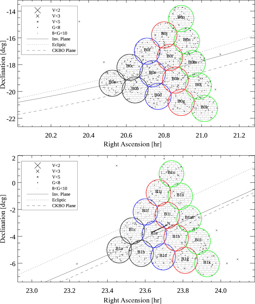
Figure 4: The “B” semester fields, observed in the second half of each year of the survey. In year 1 the black fields (B0a-c and B1a-c) were observed. In year 2, the black fields were repeated and the blue fields (B0d-f and B1d-f) were added. In year 3, all year 2 fields in addition to the red fields (B0g-j and B1g-j) were observed. The year 4 fields (B0k-o and B1k-o), in green, were not originally anticipated as part of the survey but were added later as mitigation for telescope time losses due to operational shutdowns related to the COVID-19 pandemic. Neptune’s location though our 2022B allocated observing window is marked with an N and a line.

Most of the populations of interest are thought to be relatively uniform in ecliptic longitude (classical TNOs, Scattered TNOs, Non-Hilda Asteroids, Centaurs). Exceptions to this are the Resonant TNOs, Trojan Asteroids and the Extreme TNOs which may be affected by the action of a distant massive planet (Trujillo & Sheppard, 2014). The four most populated Neptune resonances, in order of total number of observed objects in each resonance, are the 3:2, 2:1, 5:2 and 4:3. Examples of orbits of objects in the 3:2, 2:1 and 4:3 resonances can be seen in (Figures 3–10, Malhotra, 1996).

The most important point of the longitudinal distributions of the resonant objects is that the 3:2 objects, which are by far the most numerous, librate with their perihelia about 90 degrees from Neptune, with a spread of about $\pm 15$ degrees. The 2:1 objects can be found at many longitudes without introducing significant bias and the 4:3 come to perihelion 60 degrees from Neptune. So ideal field locations would probe the area about 90 degrees from Neptune. This would allow enhanced sensitivity to the smallest TNOs which would be the Neptune-crossing 3:2 objects near perihelion. A secondary field could be done 60 degrees from Neptune which would allow the 4:3 objects to be probed and provide some sensitivity to Neptune Trojans. The benefit of catching the 3:2 objects at perihelion versus aphelion is, for an object with eccentricity $e$, in terms of magnitude is $2.5\log(\frac{1+e}{1-e})^{4}=10\log\frac{1+e}{1-e}$. So for a 3:2 TNO with a typical eccentricity of 0.23, the gain is $\Delta m$ = 2.0 magnitudes in brightness. In terms of object numbers, for shallow size distributions such as the Bernstein et al. (2004) faint Hubble-detected objects, the total number of objects is proportional to $10^{\alpha\Delta m}$ where $\alpha=0.32$, so this is about a factor 4 in terms of object numbers. This also means we can probe objects that are about a factor 2.5 smaller in size using this methodology. That said, eccentric bodies do spend more time at aphelion than perihelion, so there will be an effect on survey sensitivity due to this issue, which we have not considered here.

Since the 3:2 TNOs have perihelion $90\pm 15$ degrees ($6\pm 1$ hours) from Neptune and the 4:3 TNOs are $60\pm 15$ and $180\pm 15$ degrees ($4\pm 1$ and $12\pm 1$ hours) from Neptune, this would suggest the optimum field locations should be about 05:15 and 17:15 for the 3:2 objects and 04:15, 11:15 and 19:15 for the 4:3 objects. For the 2019A semester, it was difficult to reach these resonant locations at opposition, but we could image one of the 3:2 locations. The 2019B semester provided a better opportunity although, in the end, we chose to optimize fields based on observing date and opposition proximity in the B semester (Section 3.7). The Extreme TNOs (Sheppard et al., 2019) appear to come to perihelion in the 3 to 6 RA hour range, so they were unavailable until mid-2019B. Additionally, our main science goals are related to the general TNO population which has very large expected discovery numbers, without an undue focus on the Extreme TNOs, which are much more difficult to detect (Trujillo & Sheppard, 2014), so we decided to not alter our survey fields just for the few Extreme TNOs that we might find in the survey fields.

In summary, the actual field locations were chosen to lie along the invariable plane as defined by Souami & Souchay (2012b) and designed such that equal amounts of time could be spent on each field during the on-opposition and off-opposition observations given our 2019 A semester observation dates. A similar methodology was followed for the 2019 B field choices. Subsequent years after 2019 were solely based on our initial 2019 field choices.

3.6.1 Actual Field Coordinates Selected for 2019 A Semester

Based on the approximate field centers above, we examined star locations from the Gaia catalog to select fields minimizing the number of stars brighter than $G<8$ (Gaia Collaboration et al., 2016, 2018) and in particular the especially bright stars with $V<5$. We have examined the final year 4 field configuration which is 15 full fields. The sky plots of the fields are pictured in Figure 3 and 4. All fields were moved less than 0.5 hours along the invariable plane to avoid the brightest stars. We used the invariable plane defined by Souami & Souchay (2012a) ($i=23.008861\arcdeg$ and $\Omega=3.8526111\arcdeg$ with respect to the celestial ICRF plane and $i=1.5786944\arcdeg$ and $\Omega=107.58222\arcdeg$ with respect to the J2000 ecliptic). Volk & Malhotra (2017) found that the classical TNOs had $1\sigma$ limits of $i=1.2$–$2.2\arcdeg$ and $\Omega=$63–$95\arcdeg$, which is less than the maximum deviation from the invariable plane of our field locations especially considering the cold classical TNOs have an inclination distribution that is $\sin(i)$ times a Gaussian with $1\sigma=2\arcdeg$ Gulbis et al. (2010). More recently, Matheson & Malhotra (2023) provided improved estimates of the Kuiper Belt mean plane, which for many heliocentric distances, fall within our original design criteria. The actual field coordinates are given here for our 2019 observing epoch. Note that at each observation epoch in subsequent years, field coordinates were adjusted based on the day of the year of observations and the expected apparent motion of TNOs to minimize the loss of objects moving off of field edges due to apparent motion caused by the Earth. Any orbital motion of the TNOs was not accounted for in this manner because the overall field “fan shape” was selected to adjust for the orbital motion expected for the objects.

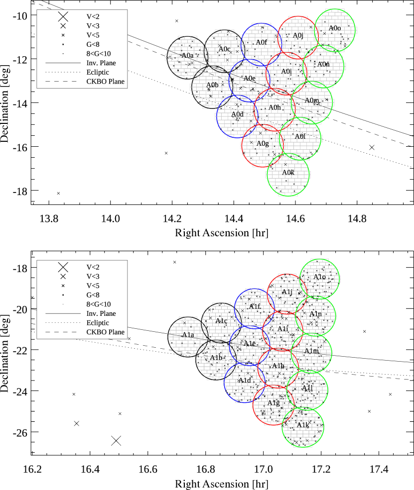
Figure 3: The “A” semester fields, observed in the first half of each year of the survey. In year 1 the black fields (A0a-c and A1a-c) were observed. In year 2, the black fields were repeated and the blue fields (A0d-f and A1d-f) were added. In year 3, all year 2 fields in addition to the red fields (A0g-j and A1g-j) were observed. The year 4 fields (A0k-o and A1k-o), in green, were not originally anticipated as part of the survey but were added later as mitigation for telescope time losses due to operational shutdowns related to the COVID-19 pandemic.

In 2019, we initially planned for 3 fields where all detected objects would be further followed in our years-long survey. As the actual fields observed each year were adjusted based on typical TNO apparent motion, and the total duration of the survey was extended due to COVID, the final field selection was not set until the 2022 observations. These field coordinates are shown for the 2022A semester in Table 4.

3.7 Actual Field Coordinates Selected for 2019 B Semester

The choice of B semester fields was largely based on our allocation of telescope time in the first semester of observations following the same methodology of the A semester observations. Given that we were allocated telescope time in 2019 in late August and late September, we planned our fields so that both the opposition and quadrature observations were available during those time periods — for the early fields, opposition in late August and quadrature in late September, and for the late fields, quadrature in late August and opposition in late September. Given these constraints, plus the goal of avoiding bright stars and the fact that the full field pattern of 15 fields wasn’t determined until 2022, we report the 2022 epoch fields in Table 5 for the B semester.

Table 3: Summary of field observations for the DEEP project as of 2022B. Sky coordinates are given as right ascension ($\alpha$) and declination ($\delta$). The value $t_{\rm eff}\approx 1$ is an empirical measure of efficiency roughly consistent with seeing full-width-at-half-maximum of 0.95 arc-seconds under clear, moonless skies – optimal conditions with DECam, which is described in detail in Equation 4 of Morganson et al. (2018). $N$ is number of 120 s observations, $\chi$ is mean airmass, $\theta$ is mean seeing full-width-at-half-maximum, $m_{\rm sky}$ is mean sky brightness, and $m_{\rm ext}$ is mean extinction. Computations were performed with algorithms supplied as part of the Dark Energy Survey Image Processing Pipeline (Morganson et al., 2018).

Local Date	Night	UT Time	Field	$\alpha$	$\delta$	$N$	$t_{\rm eff}$	$\chi$	$\theta$	$m_{\rm sky}$	$m_{\rm ext}$
Start of Night	Fraction	Range	Name	[°]	[°]				[″]
2019/04/01	second half	05:13–05:18,09:36–09:41	A0c	216.5	-12.0	6	2.32	1.29	1.52	0.02	0.00
2019/04/01	second half	05:21–09:22	A0a	214.7	-12.3	98	53.33	1.14	1.37	0.00	0.00
2019/04/01	second half	05:06–05:11,09:25–09:33	A0b	215.9	-13.6	7	2.78	1.28	1.49	0.01	0.07
2019/04/02	second half	05:09–09:22	A0b	215.9	-13.6	103	65.19	1.12	1.27	0.00	0.00
2019/04/02	second half	04:53–04:58,09:24–09:30	A0a	214.7	-12.3	6	3.32	1.29	1.35	0.00	0.00
2019/04/02	second half	05:01–05:06,09:32–09:37	A0c	216.5	-12.0	6	3.39	1.30	1.33	0.00	0.00
2019/04/03	second half	05:07–09:24	A0c	216.5	-12.0	104	31.37	1.14	1.70	0.07	0.00
2019/04/03	second half	04:47,09:28–09:37	A0a	214.7	-12.3	5	0.84	1.45	2.44	0.33	0.00
2019/04/03	second half	05:00–05:05,09:39–10:00	A0b	215.9	-13.6	12	1.94	1.47	2.16	0.57	0.15
2019/05/03	full night	01:02–04:38	A0a	214.7	-12.3	88	51.40	1.16	1.02	0.40	0.00
2019/05/03	full night	00:47–00:52,04:41–04:46	A0b	215.9	-13.6	6	3.39	1.31	1.04	0.44	0.00
2019/05/03	full night	00:55–01:00,04:48–04:53	A0c	216.5	-12.0	6	3.00	1.31	1.10	0.42	0.00
2019/05/03	full night	06:15–09:17	A1a	251.6	-21.5	74	54.28	1.07	0.93	0.37	0.00
2019/05/03	full night	06:00,09:49–09:54	A1b	253.1	-22.6	4	1.92	1.27	1.04	0.58	0.00
2019/05/03	full night	06:07–06:12,09:19–09:46	A1c	253.4	-20.8	15	6.30	1.23	1.05	0.59	0.25
2019/05/04	full night	00:39–00:44,04:40–04:45	A0a	214.7	-12.3	6	2.94	1.32	1.27	0.16	0.00
2019/05/04	full night	00:47–00:52,04:48–04:53	A0b	215.9	-13.6	6	2.98	1.30	1.23	0.20	0.04
2019/05/04	full night	00:54–04:38	A0c	216.5	-12.0	91	52.84	1.18	1.13	0.10	0.00
2019/05/04	full night	06:01–06:06,09:38–09:43	A1a	251.6	-21.5	5	1.70	1.19	1.29	0.29	1.23
2019/05/04	full night	06:09–06:14,09:46–09:50	A1b	253.1	-22.6	6	1.54	1.18	1.26	0.42	2.34
2019/05/04	full night	06:16–09:36	A1c	253.4	-20.8	70	4.88	1.09	1.23	0.49	2.49
2019/05/05	full night	no data collected	—	—	—	—	—	—	—	—	—
2019/05/06	full night	00:52–00:57,04:40–04:45	A0a	214.7	-12.3	6	5.29	1.26	1.00	0.09	0.00
2019/05/06	full night	01:07–04:38	A0b	215.9	-13.6	86	23.68	1.13	0.99	0.22	1.22
2019/05/06	full night	00:59–01:04,04:48–04:53	A0c	216.5	-12.0	6	5.82	1.26	0.97	0.07	0.00
2019/05/06	full night	05:58–06:03,09:40	A1a	251.6	-21.5	4	0.11	1.11	1.10	0.40	3.29
2019/05/06	full night	06:13–09:37	A1b	253.1	-22.6	79	27.93	1.09	1.03	0.37	1.09
2019/05/06	full night	06:06–06:11,09:47	A1c	253.4	-20.8	4	0.07	1.12	1.02	0.42	3.13
2019/06/01	first half	00:09–00:14	A1a	251.0	-21.4	3	0.69	2.12	1.59	0.47	0.00
2019/06/01	first half	00:24–04:38	A1b	252.5	-22.5	99	63.78	1.29	1.09	0.21	0.00
2019/06/01	first half	00:16–00:21	A1c	252.8	-20.7	3	0.78	2.13	1.47	0.49	0.00
2019/06/02	first half	23:25–23:33	A0a	213.6	-11.9	4	1.40	1.35	0.92	1.10	0.00
2019/06/02	first half	00:40–04:37	A1a	251.0	-21.4	96	71.78	1.22	1.04	0.11	0.00
2019/06/03	first half	23:31–23:58	A0a	213.6	-11.9	12	7.31	1.28	0.98	0.35	0.00
2019/06/03	first half	00:04–00:09,04:22–04:29	A1a	251.0	-21.4	8	2.97	1.41	1.43	0.17	0.00
2019/06/03	first half	00:14–00:16,04:34–04:39	A1b	252.5	-22.5	6	2.40	1.52	1.31	0.26	0.05
2019/06/03	first half	00:19–04:19	A1c	252.8	-20.7	97	28.39	1.31	1.46	0.21	0.41
2019/07/06	second half	04:49–07:17	B0a	308.8	-19.2	60	2.11	1.04	1.37	0.23	2.33
2019/07/06	second half	04:33–04:39	B0b	310.6	-19.7	3	1.29	1.13	1.52	0.00	0.13
2019/07/06	second half	04:41–04:46	B0c	310.2	-18.0	3	0.58	1.11	1.78	0.01	0.44
2019/07/07	second half	05:11–08:32	B0a	308.8	-19.2	80	2.65	1.06	1.44	0.09	2.15
2019/07/07	second half	04:55–05:01	B0b	310.6	-19.7	3	0.07	1.08	1.40	0.14	1.98
2019/07/07	second half	05:03–05:06	B0c	310.2	-18.0	2	0.00	1.08	1.54	0.24	3.26
2019/07/08	second half	05:12–10:31	B0a	308.8	-19.2	121	11.99	1.20	1.14	0.30	2.37
2019/07/08	second half	04:55–05:01,09:59-10:05	B0b	310.6	-19.7	6	0.61	1.34	1.42	0.26	2.21
2019/07/08	second half	05:04–05:10,10:07-10:12	B0c	310.2	-18.0	6	0.35	1.38	1.36	0.33	2.41
2019/08/27	full night	23:35–23:40,04:37–04:42	B0a	307.8	-19.4	6	5.12	1.27	1.05	0.11	0.00
2019/08/27	full night	23:15–23:32,04:29–04:34	B0b	309.6	-19.9	11	5.20	1.42	1.28	0.93	0.19
2019/08/27	full night	23:42–04:26	B0c	309.2	-18.2	115	98.31	1.11	1.06	0.00	0.00
2019/08/27	full night	04:57–04:59,09:27–09:32	B1a	351.9	-5.0	6	5.60	1.51	1.00	0.15	0.00
2019/08/27	full night	04:46–04:52,09:20–09:25	B1b	353.6	-5.3	6	5.06	1.44	1.02	0.12	0.00
2019/08/27	full night	05:02–09:17	B1c	352.9	-3.6	103	62.55	1.27	1.17	0.06	0.06
2019/08/28	full night	23:43–04:27	B0a	307.8	-19.4	115	135.40	1.10	0.95	0.00	0.00
2019/08/28	full night	23:35–23:40,04:39–04:44	B0b	309.6	-19.9	6	5.96	1.27	1.00	0.00	0.00
2019/08/28	full night	23:14–23:33,04:29–04:34	B0c	309.2	-18.2	9	5.96	1.38	1.02	0.81	0.00
2019/08/28	full night	05:03–09:15	B1a	351.9	-5.0	102	53.31	1.27	1.48	0.00	0.00
2019/08/28	full night	04:45–05:01,09:28–09:33	B1b	353.6	-5.3	6	4.06	1.49	1.28	0.01	0.00
2019/08/28	full night	04:48–04:53,09:18–09:25	B1c	352.9	-3.6	7	4.67	1.55	1.28	0.05	0.00
2019/08/29	full night	23:17–23:34,04:28–04:35	B0a	307.8	-19.4	12	6.60	1.33	1.15	0.76	0.00
2019/08/29	full night	23:45–04:26	B0b	309.6	-19.9	114	121.76	1.10	1.00	0.00	0.00
2019/08/29	full night	23:36–23:41,04:38–04:43	B0c	309.2	-18.2	6	5.65	1.27	1.01	0.00	0.00
2019/08/29	full night	04:47–04:54,09:18–09:25	B1a	351.9	-5.0	8	6.57	1.51	1.17	0.00	0.00
2019/08/29	full night	05:04–09:15	B1b	353.6	-5.3	101	113.41	1.25	0.98	0.00	0.00
2019/08/29	full night	04:56–05:01,09:30–09:33	B1c	352.9	-3.6	6	5.33	1.56	1.12	0.00	0.00
2019/09/26	first half	00:19–04:16	B1a	351.4	-5.2	97	57.57	1.26	1.25	0.00	0.00
2019/09/26	first half	00:04–00:09,04:23–04:28	B1b	353.1	-5.5	6	1.40	1.52	1.88	0.22	0.00
2019/09/26	first half	00:11–00:16,04:18–04:21	B1c	352.4	-3.8	5	1.43	1.57	1.62	0.21	0.00
2019/09/27	first half	00:01–00:06,04:17–04:22	B1a	351.4	-5.2	6	1.74	1.49	1.77	0.37	0.00
2019/09/27	first half	00:16–04:14	B1b	353.1	-5.5	97	48.07	1.28	1.28	0.22	0.00
2019/09/27	first half	00:08–00:13,04:24–04:29	B1c	352.4	-3.8	6	1.86	1.50	1.69	0.38	0.00
2019/09/28	first half	00:02–00:07,04:17–04:22	B1a	351.4	-5.2	6	5.25	1.46	1.07	0.10	0.00
2019/09/28	first half	00:10–00:15,04:24–04:29	B1b	353.1	-5.5	6	5.14	1.46	1.10	0.08	0.00
2019/09/28	first half	00:18–04:13	B1c	352.4	-3.8	96	84.00	1.28	1.06	0.00	0.00
2020/04/18	second half	no data collected	—	—	—	—	—	—	—	—	—
2020/04/19	second half	no data collected	—	—	—	—	—	—	—	—	—
2020/04/20	second half	no data collected	—	—	—	—	—	—	—	—	—
2020/04/21	second half	no data collected	—	—	—	—	—	—	—	—	—
2020/04/22	second half	no data collected	—	—	—	—	—	—	—	—	—
2020/04/23	second half	no data collected	—	—	—	—	—	—	—	—	—
2020/05/17	second half	no data collected	—	—	—	—	—	—	—	—	—
2020/05/18	second half	no data collected	—	—	—	—	—	—	—	—	—
2020/05/19	second half	no data collected	—	—	—	—	—	—	—	—	—
2020/05/20	second half	no data collected	—	—	—	—	—	—	—	—	—
2020/05/21	second half	no data collected	—	—	—	—	—	—	—	—	—
2020/05/22	second half	no data collected	—	—	—	—	—	—	—	—	—
2020/10/15	first half	23:58–04:11	B1b	352.9	-5.6	103	59.94	1.17	1.38	0.00	0.00
2020/10/15	first half	23:53–23:56,04:14–04:18	B1c	352.2	-3.9	6	3.38	1.34	1.16	0.39	0.00
2020/10/15	first half	23:43–23:48,04:21–04:26	B1e	353.9	-4.2	6	2.57	1.37	1.28	0.99	0.00
2020/10/16	first half	23:43–23:48,04:12–04:17	B1b	352.9	-5.6	6	2.84	1.33	1.08	1.17	0.00
2020/10/16	first half	00:13–04:09	B1c	352.2	-3.9	96	84.45	1.17	1.07	0.00	0.00
2020/10/16	first half	23:58–00:03	B1d	354.6	-5.9	3	1.37	1.40	1.16	0.41	0.00
2020/10/16	first half	23:51–23:56,04:19–04:24	B1e	353.9	-4.2	6	3.32	1.34	1.13	0.53	0.00
2020/10/16	first half	00:06–00:11	B1f	353.2	-2.5	3	1.87	1.39	1.11	0.15	0.00
2020/10/17	first half	23:45–23:50,04:14–04:19	B1b	352.9	-5.6	6	3.48	1.32	1.17	1.02	0.00
2020/10/17	first half	23:52–23:58,04:21–04:26	B1c	352.2	-3.9	6	3.26	1.34	1.16	0.40	0.00
2020/10/17	first half	00:00–00:05	B1d	354.6	-5.9	3	1.16	1.37	1.25	0.41	0.00
2020/10/17	first half	00:15–04:12	B1e	353.9	-4.2	95	88.66	1.17	1.03	0.00	0.00
2020/10/17	first half	00:08–00:13	B1f	353.2	-2.5	3	1.50	1.37	1.23	0.16	0.00
2020/10/18	first half	00:20–04:04	B1a	351.1	-5.3	91	104.06	1.15	0.89	0.00	0.00
2020/10/18	first half	00:11–00:16	B1b	352.9	-5.6	3	3.14	1.29	0.84	0.18	0.00
2020/10/18	first half	23:48–23:53,04:06–04:11	B1d	354.6	-5.9	6	2.91	1.31	1.06	0.83	0.00
2020/10/18	first half	23:56–00:01,04:14–04:18	B1e	353.9	-4.2	6	3.41	1.32	1.06	0.38	0.00
2020/10/18	first half	00:03–00:08,04:21–04:26	B1f	353.2	-2.5	6	4.32	1.33	1.02	0.18	0.00
2020/10/19	first half	23:49–23:54,04:09–04:17	B1a	351.1	-5.3	7	1.76	1.30	1.56	0.74	0.00
2020/10/19	first half	23:56–00:01,04:19–04:24	B1c	352.2	-3.9	6	2.32	1.32	1.35	0.45	0.00
2020/10/19	first half	00:04–04:07	B1d	354.6	-5.9	99	51.48	1.16	1.24	0.16	0.00
2020/10/20	first half	23:47–23:59,04:11–04:21	B1b	352.9	-5.6	6	2.61	1.30	1.27	0.90	0.00
2020/10/20	first half	23:52–00:02,04:14–04:24	B1e	353.9	-4.2	6	2.87	1.32	1.24	0.69	0.00
2020/10/20	first half	00:04–04:09	B1f	353.2	-2.5	98	64.84	1.19	1.10	0.20	0.00
2020/10/21	first half	23:49–23:59,04:11–04:22	B1a	351.1	-5.3	7	3.30	1.30	1.04	0.86	0.00
2020/10/21	first half	23:51–00:01,04:14–04:24	B1c	352.2	-3.9	6	2.61	1.32	1.10	0.82	0.00
2020/10/21	first half	00:04–04:08	B1d	354.6	-5.9	99	75.08	1.15	0.96	0.27	0.00
2021/05/03	first half	00:28–00:33,04:34–04:39	A0f	217.7	-11.5	6	1.04	1.46	2.09	0.18	0.00
2021/05/03	first half	00:14–00:26,04:24–04:31	A0i	218.9	-12.8	8	1.53	1.53	2.03	0.18	0.15
2021/05/03	first half	00:36–04:22	A0j	219.5	-11.2	92	29.16	1.30	1.83	0.00	0.05
2021/05/04	first half	02:29–04:38	A0f	217.7	-11.5	53	26.49	1.09	1.48	0.00	0.00
2021/05/05	no time scheduled	no data collected	—	—	—	—	—	—	—	—	—
2021/05/06	full night	00:20–01:52	A0i	218.9	-12.8	26	0.08	1.51	1.68	0.47	3.12
2021/05/06	full night	02:54–10:30	A1j	256.7	-19.3	179	22.10	1.19	1.69	0.39	1.88
2021/05/07	full night	23:53–00:00,05:18–05:24	A0e	217.1	-13.1	6	0.29	1.55	1.90	0.34	2.01
2021/05/07	full night	00:04–05:05	A0i	218.9	-12.8	121	43.06	1.26	1.54	0.05	0.26
2021/05/07	full night	23:46–23:51,05:09–05:14	A0j	219.5	-11.2	6	0.42	1.72	1.68	0.33	1.14
2021/05/07	full night	05:36–05:41	A1e	254.7	-21.9	2	0.00	1.04	1.31	0.33	5.57
2021/05/07	full night	05:45–10:28	A1f	255.0	-20.1	88	0.39	1.17	1.35	0.65	3.87
2021/05/07	full night	05:28–05:34	A1i	256.4	-21.1	3	0.00	1.06	1.42	0.42	3.41
2021/05/08	no time scheduled	no data collected	—	—	—	—	—	—	—	—	—
2021/05/09	full night	23:55–02:39	A0g	217.8	-16.1	66	5.03	1.37	1.33	0.40	2.07
2021/05/09	full night	06:21–06:24,10:20–10:25	A1e	254.7	-21.9	5	0.33	1.39	1.07	1.52	0.86
2021/05/09	full night	06:26–10:10	A1f	255.0	-20.1	68	5.61	1.18	1.06	0.60	1.83
2021/05/09	full night	06:11–06:16,10:13-10:18	A1i	256.4	-21.1	6	0.32	1.28	1.14	0.86	1.35
2021/05/10	full night	23:59–00:10,04:01–04:06	A0a	214.1	-12.1	7	4.68	1.41	1.18	0.03	0.00
2021/05/10	full night	00:13–00:18,04:08–04:13	A0b	215.3	-13.4	6	4.56	1.34	1.10	0.02	0.00
2021/05/10	full night	00:20–03:53	A0c	215.9	-11.8	73	58.44	1.21	1.09	0.00	0.00
2021/05/10	full night	04:17–04:22,10:17–10:22	A1c	253.2	-20.8	6	2.68	1.43	1.42	0.73	0.05
2021/05/10	full night	04:35–06:59	A1f	255.0	-20.1	40	25.38	1.04	1.15	0.11	0.14
2021/05/10	full night	10:25–10:30	A1h	256.2	-22.9	3	0.11	1.64	1.53	2.57	0.00
2021/05/10	full night	08:06–10:15	A1i	256.4	-21.1	45	12.95	1.30	1.47	0.44	0.10
2021/05/11	no time scheduled	no data collected	—	—	—	—	—	—	—	—	—
2021/05/12	full night	23:01–23:03,01:05–01:10	A0a	214.1	-12.1	5	1.30	1.74	1.54	0.48	0.14
2021/05/12	full night	01:12–01:15	A0c	215.9	-11.8	2	1.07	1.30	1.21	0.14	0.00
2021/05/12	full night	01:20–01:59	A0e	217.1	-13.1	17	9.22	1.21	1.06	0.13	0.35
2021/05/13	full night	23:24–23:29	A0b	215.3	-13.4	3	1.28	1.99	1.15	0.48	0.00
2021/05/13	full night	23:32–23:37	A0d	216.6	-14.8	3	1.54	1.92	1.07	0.44	0.05
2021/05/13	full night	23:39–03:45	A0e	217.1	-13.1	100	110.09	1.28	0.91	0.01	0.00
2021/05/13	full night	03:49–07:10	A1c	253.2	-20.8	82	94.55	1.06	0.87	0.03	0.00
2021/05/13	full night	07:17–10:30	A1e	254.7	-21.9	48	28.99	1.33	1.11	0.40	0.07
2021/05/14	no time scheduled	no data collected	—	—	—	—	—	—	—	—	—
2021/05/15	full night	02:15–06:33	A0h	218.4	-14.4	101	66.56	1.11	1.19	0.01	0.12
2021/05/15	full night	06:37–10:31	A1h	256.2	-22.9	74	27.91	1.27	1.33	0.40	0.21
2021/05/16	full night	23:18–03:09	A0a	214.1	-12.1	94	70.16	1.30	1.04	0.16	0.00
2021/05/16	full night	03:28–06:48	A0b	215.3	-13.4	79	72.86	1.19	0.99	0.00	0.00
2021/05/16	full night	22:48–22:53,03:13–03:18	A0d	216.6	-14.8	6	2.01	1.72	1.30	1.26	0.15
2021/05/16	full night	22:56–23:01,03:20–03:25	A0g	217.8	-16.1	6	2.30	1.67	1.29	0.69	0.15
2021/05/16	full night	06:52–10:30	A1a	251.5	-21.4	89	53.49	1.39	1.07	0.43	0.00
2021/05/17	no time scheduled	no data collected	—	—	—	—	—	—	—	—	—
2021/05/18	second half	04:38–04:43	A1a	251.5	-21.4	3	0.56	1.04	2.00	0.00	0.44
2021/05/18	second half	04:53–04:58	A1b	253.0	-22.6	3	0.79	1.03	1.88	0.00	0.26
2021/05/18	second half	05:23–07:43	A1d	254.5	-23.7	57	2.96	1.03	1.74	0.19	1.58
2021/05/18	second half	05:01–05:05	A1e	254.7	-21.9	3	0.23	1.03	2.23	0.00	0.76
2021/05/18	second half	05:10–05:13	A1f	255.0	-20.1	2	0.11	1.03	2.47	0.00	0.81
2021/05/18	second half	04:46–04:51	A1h	256.2	-22.9	3	0.45	1.05	2.32	0.00	0.29
2021/05/18	second half	05:15–05:20	A1j	256.7	-19.3	3	0.08	1.03	2.55	0.02	1.05
2021/05/19	second half	no data collected	—	—	—	—	—	—	—	—	—
2021/09/03	first half	23:25–02:07	B0b	309.4	-19.9	66	31.86	1.13	1.44	0.00	0.08
2021/09/03	first half	02:11–04:40	B1f	353.8	-2.3	61	24.51	1.34	1.66	0.00	0.00
2021/09/04	first half	23:21–02:12	B0a	307.6	-19.4	70	49.42	1.12	1.18	0.03	0.00
2021/09/04	first half	02:16–04:40	B1e	354.5	-3.9	59	35.91	1.30	1.33	0.00	0.00
2021/09/05	first half	23:21–00:14	B0a	307.6	-19.4	12	6.06	1.22	1.11	0.56	0.00
2021/09/05	first half	23:29–02:01	B0c	309.0	-18.3	52	46.85	1.10	0.98	0.08	0.00
2021/09/05	first half	02:05–02:25	B1e	354.5	-3.9	6	3.14	1.60	1.26	0.08	0.00
2021/09/05	first half	02:12–02:32	B1f	353.8	-2.3	6	3.61	1.56	1.18	0.05	0.00
2021/09/05	first half	02:35–04:41	B1i	355.5	-2.5	52	28.12	1.29	1.40	0.00	0.05
2021/09/06	first half	23:22–23:27	B0c	309.0	-18.3	3	0.47	1.32	1.25	1.49	0.00
2021/09/06	first half	23:29–02:18	B0f	310.4	-17.1	69	41.17	1.12	1.23	0.01	0.05
2021/09/06	first half	02:30–04:39	B1c	352.8	-3.7	53	30.45	1.24	1.29	0.00	0.00
2021/09/06	first half	02:22–02:27	B1i	355.5	-2.5	3	1.17	1.55	1.43	0.11	0.08
2021/09/07	first half	23:25–23:30	B0a	307.6	-19.4	3	0.03	1.26	5.13	1.18	0.19
2021/09/07	first half	23:33–02:04	B0d	311.3	-20.4	62	3.19	1.11	4.54	0.00	0.15
2021/09/07	first half	02:08–02:13	B1c	352.8	-3.7	3	0.03	1.53	7.94	0.00	0.12
2021/09/07	first half	02:16–04:37	B1h	356.2	-4.2	58	2.02	1.29	5.83	0.00	0.00
2021/09/08	first half	23:22–23:27	B0a	307.6	-19.4	3	0.36	1.25	1.18	1.83	0.00
2021/09/08	first half	23:29–01:11	B0d	311.3	-20.4	42	15.13	1.14	1.37	0.32	0.16
2021/09/08	first half	01:36–01:41	B1c	352.8	-3.7	3	1.24	1.73	1.25	0.34	0.02
2021/09/08	first half	01:44–04:35	B1h	356.2	-4.2	70	32.49	1.35	1.36	0.06	0.08
2021/09/09	first half	23:35–23:50	B0a	307.6	-19.4	4	4.40	1.18	0.83	0.19	0.00
2021/09/09	first half	00:00–01:37	B0c	309.0	-18.3	40	50.56	1.08	0.83	0.02	0.00
2021/09/09	first half	23:53–23:58	B0d	311.3	-20.4	3	2.37	1.18	1.41	0.14	0.00
2021/09/09	first half	23:38–23:43	B0f	310.4	-17.1	3	2.98	1.24	0.85	0.21	0.00
2021/09/09	first half	01:57–04:36	B1a	351.7	-5.1	65	63.82	1.24	1.08	0.00	0.00
2021/09/09	first half	01:42–01:47	B1b	353.5	-5.4	3	1.77	1.63	1.23	0.00	0.00
2021/09/09	first half	01:50–01:55	B1e	354.5	-3.9	3	2.30	1.64	1.08	0.00	0.00
2021/09/10	first half	23:19–00:59	B0a	307.6	-19.4	41	3.93	1.12	1.08	1.08	1.95
2021/09/10	first half	01:05–04:06	B1a	351.7	-5.1	66	10.51	1.36	1.05	0.24	2.20
2021/09/11	first half	no data collected	—	—	—	—	—	—	—	—	—
2021/09/12	first half	23:24–01:14	B0e	310.8	-18.7	45	14.32	1.12	1.33	0.68	0.01
2021/09/12	first half	01:18–04:09	B1b	353.5	-5.4	70	20.78	1.33	1.52	0.39	0.03
2021/09/27	first half	00:16–03:54	B1d	354.8	-5.8	89	78.75	1.30	1.03	0.00	0.00
2021/09/27	first half	00:01–00:06,04:04–04:09	B1g	356.5	-6.0	6	3.78	1.58	1.22	0.11	0.00
2021/09/27	first half	23:53–00:14,03:57–04:02	B1j	354.4	-1.0	9	4.39	1.80	1.25	0.27	0.00
2021/09/28	first half	00:05–00:09,04:00–04:05	B1d	354.8	-5.8	6	3.81	1.49	1.30	0.13	0.24
2021/09/28	first half	00:12–03:57	B1g	356.5	-6.0	92	62.64	1.32	1.05	0.10	0.29
2021/09/28	first half	23:57–00:02,04:07–04:12	B1j	354.4	-1.0	6	4.15	1.64	1.19	0.19	0.03
2021/09/29	first half	no data collected	—	—	—	—	—	—	—	—	—
2021/09/30	first half	00:11–00:16,03:58–04:05	B1d	354.8	-5.8	7	1.58	1.37	2.03	0.22	0.05
2021/09/30	first half	00:20–00:24,04:07–04:12	B1g	356.5	-6.0	6	1.27	1.41	1.86	0.24	0.00
2021/09/30	first half	00:27–03:55	B1j	354.4	-1.0	85	33.11	1.31	1.46	0.22	0.00
2021/10/01	first half	00:37–03:56	B1b	353.1	-5.5	81	84.68	1.21	0.88	0.14	0.00
2021/10/01	first half	00:20–00:27,03:58–04:06	B1f	353.4	-2.4	8	8.55	1.40	0.86	0.29	0.00
2021/10/01	first half	00:30–00:35,04:08–04:13	B1i	355.1	-2.7	6	5.96	1.39	0.88	0.30	0.00
2021/10/02	first half	23:58–00:05,03:58–04:06	B1b	353.1	-5.5	8	5.73	1.42	1.01	0.30	0.00
2021/10/02	first half	00:15–03:56	B1f	353.4	-2.4	89	84.73	1.27	0.90	0.19	0.00
2021/10/02	first half	00:08–00:13,04:08–04:13	B1i	355.1	-2.7	6	4.51	1.47	0.99	0.29	0.00
2021/10/03	first half	23:28–23:46,04:13	B1b	353.1	-5.5	4	1.40	1.69	1.12	1.28	0.00
2021/10/03	first half	23:50–23:58	B1f	353.4	-2.4	3	0.94	1.85	1.58	0.59	0.00
2021/10/03	first half	00:02–04:10	B1i	355.1	-2.7	100	84.57	1.30	0.99	0.10	0.00
2021/10/04	first half	23:58–04:08	B1c	352.4	-3.9	101	81.26	1.25	1.11	0.00	0.00
2021/10/04	first half	23:39–23:48	B1e	354.1	-4.1	4	0.50	1.91	1.36	1.60	0.00
2021/10/04	first half	23:50–23:55,04:10–04:15	B1h	355.8	-4.4	6	5.44	1.50	1.04	0.25	0.04
2021/10/05	first half	23:44–23:52,04:02–04:07	B1c	352.4	-3.9	7	3.70	1.49	1.28	0.68	0.00
2021/10/05	first half	23:54–23:59,04:10–04:15	B1e	354.1	-4.1	6	4.69	1.44	1.00	0.36	0.00
2021/10/05	first half	00:02–04:00	B1h	355.8	-4.4	97	73.04	1.27	1.02	0.17	0.01
2021/10/06	first half	23:50-23:55,04:05–04:10	B1c	352.4	-3.9	5	2.51	1.48	1.17	0.53	0.00
2021/10/06	first half	00:05–04:03	B1e	354.1	-4.1	97	72.75	1.24	1.09	0.07	0.00
2021/10/06	first half	23:57–00:02,04:08–04:13	B1h	355.8	-4.4	5	2.58	1.49	1.16	0.36	0.02
2022/05/25	first half	23:04–02:05	A0a	213.7	-12.0	74	79.04	1.27	0.84	0.21	0.00
2022/05/25	first half	22:50–22:59,04:33–04:38	A0b	215.0	-13.3	6	4.26	1.48	0.96	1.07	0.00
2022/05/25	first half	22:52–04:30	A0f	217.3	-11.4	61	75.58	1.12	0.77	0.04	10.87
2022/05/26	first half	22:53–23:23	A0a	213.7	-12.0	5	1.38	1.64	1.28	1.06	0.00
2022/05/26	first half	23:26–02:19	A0b	215.0	-13.3	71	79.08	1.21	0.88	0.09	0.00
2022/05/26	first half	22:51–04:38	A0c	215.5	-11.7	61	79.44	1.14	0.86	0.03	0.00
2022/05/26	first half	22:48–23:18	A0f	217.3	-11.4	5	-0.16	1.83	1.28	1.58	19.55
2022/05/27	first half	22:47–23:09	A0a	213.7	-12.0	4	0.07	1.69	0.95	1.96	24.27
2022/05/27	first half	22:49–23:12	A0b	215.0	-13.3	4	1.33	1.68	0.92	1.66	0.00
2022/05/27	first half	22:52–23:14	A0c	215.5	-11.7	4	1.49	1.72	0.94	1.40	0.00
2022/05/27	first half	23:16–02:12	A0d	216.2	-14.6	72	83.21	1.22	0.87	0.08	0.00
2022/05/27	first half	02:14–04:38	A0e	216.8	-13.0	59	68.77	1.08	0.86	0.05	0.00
2022/05/28	first half	no data collected	—	—	—	—	—	—	—	—	—
2022/05/29	no time scheduled	no data collected	—	—	—	—	—	—	—	—	—
2022/05/30	first half	no data collected	—	—	—	—	—	—	—	—	—
2022/05/31	first half	no data collected	—	—	—	—	—	—	—	—	—
2022/06/01	first half	no data collected	—	—	—	—	—	—	—	—	—
2022/06/02	first half	no data collected	—	—	—	—	—	—	—	—	—
2022/06/03	first half	no data collected	—	—	—	—	—	—	—	—	—
2022/06/04	first half	no data collected	—	—	—	—	—	—	—	—	—
2022/06/05	first half	no data collected	—	—	—	—	—	—	—	—	—
2022/06/06	first half	no data collected	—	—	—	—	—	—	—	—	—
2022/08/21	second half	05:04–07:43	B1a	351.9	-5.0	65	63.76	1.13	1.07	0.00	0.00
2022/08/21	second half	04:49–04:59	B1d	355.4	-5.5	3	3.18	1.19	1.04	0.00	0.00
2022/08/21	second half	07:46–10:17	B1h	356.5	-4.1	62	21.60	1.47	1.43	0.45	0.24
2022/08/21	second half	04:52–05:02	B1m	357.5	-2.7	3	3.10	1.23	1.05	0.00	0.00
2022/08/22	second half	04:50–05:01,10:05–10:10	B1a	351.9	-5.0	5	2.80	1.55	1.38	0.77	0.00
2022/08/22	second half	05:06–07:37	B1d	355.4	-5.5	62	72.37	1.12	0.96	0.00	0.00
2022/08/22	second half	07:41–10:02	B1g	357.2	-5.8	58	41.13	1.39	1.19	0.01	0.00
2022/08/22	second half	04:52–05:03,10:07–10:13	B1m	357.5	-2.7	5	2.38	1.52	1.33	0.94	0.00
2022/08/23	second half	04:51–05:07,10:00–10:08	B1a	351.9	-5.0	5	2.86	1.55	1.13	0.59	0.00
2022/08/23	second half	04:54–05:09,10:03–10:10	B1d	355.4	-5.5	5	2.73	1.49	1.13	0.73	0.03
2022/08/23	second half	04:48–05:04,09:57–10:13	B1g	357.2	-5.8	6	2.62	1.53	1.17	0.89	0.03
2022/08/23	second half	05:12–09:55	B1m	357.5	-2.7	115	95.50	1.28	1.09	0.00	0.00
2022/08/24	no time scheduled	no data collected	—	—	—	—	—	—	—	—	—
2022/08/25	second half	05:07–05:12	B1b	353.7	-5.3	3	2.87	1.13	0.80	0.02	0.40
2022/08/25	second half	05:14–09:30	B1e	354.7	-3.9	91	40.35	1.23	0.92	0.00	1.57
2022/08/25	second half	05:00–05:04	B1g	357.2	-5.8	3	3.58	1.15	0.83	0.02	0.16
2022/08/25	second half	04:49–04:57	B1k	358.9	-6.0	3	1.91	1.18	1.10	0.03	0.16
2022/08/26	second half	09:47–09:52	B1b	353.7	-5.3	3	1.64	2.00	1.07	0.38	0.00
2022/08/26	second half	09:39–09:44	B1e	354.7	-3.9	3	2.31	1.90	0.98	0.18	0.00
2022/08/26	second half	09:54–09:59	B1i	355.8	-2.4	3	0.92	2.08	1.12	0.93	0.00
2022/08/26	second half	07:03–09:37	B1k	358.9	-6.0	63	87.65	1.30	0.85	0.00	0.00
2022/08/26	second half	04:35–07:01	B1l	358.2	-4.4	60	94.09	1.14	0.85	0.00	0.00
2022/08/27	second half	04:45–07:12	B1b	353.7	-5.3	60	60.63	1.12	0.96	0.00	0.00
2022/08/27	second half	07:14–09:53	B1i	355.8	-2.4	65	52.04	1.49	0.96	0.25	0.00
2022/08/27	second half	10:03–10:08	B1k	358.9	-6.0	3	0.24	1.96	1.11	2.46	0.00
2022/08/27	second half	09:55–10:00	B1l	358.2	-4.4	3	0.63	1.96	1.10	1.37	0.00

Table 4: Field coordinates for observations in the 2022 A Semester (J2000) for 1 June 2022 UT. Field coordinates for observation at other epochs were precessed based on the date of the year to account for parallax due to the Earth’s motion. There were no adjustments made for year-to-year orbital motion because the increasing size of the fan pattern was intended to account for year-to-year orbital motion.

Field Name	RA	Dec
A0a	14:14:59.71	-11:57:03.44
A0b	14:19:49.09	-13:17:36.23
A0c	14:22:11.42	-11:39:26.43
A0d	14:24:41.45	-14:37:49.69
A0e	14:27:02.70	-12:59:30.33
A0f	14:29:22.09	-11:21:06.26
A0g	14:29:36.95	-15:57:42.78
A0h	14:31:57.11	-14:19:13.73
A0i	14:34:15.23	-12:40:39.61
A0j	14:36:31.58	-11:02:01.10
A0k	14:34:35.73	-17:17:14.45
A0l	14:36:54.80	-15:38:35.57
A0m	14:39:11.66	-13:59:51.30
A0n	14:41:26.57	-12:21:02.30
A0o	14:43:39.79	-10:42:09.21
A1a	16:44:20.49	-21:23:01.75
A1b	16:50:10.37	-22:30:03.56
A1c	16:51:16.46	-20:42:20.34
A1d	16:56:05.70	-23:36:19.26
A1e	16:57:07.87	-21:48:27.59
A1f	16:58:08.51	-20:00:34.51
A1g	17:02:06.59	-24:41:47.35
A1h	17:03:04.71	-22:53:47.66
A1i	17:04:01.31	-21:05:46.68
A1j	17:04:56.55	-19:17:44.56
A1k	17:08:13.16	-25:46:26.34
A1l	17:09:07.07	-23:58:19.08
A1m	17:09:59.48	-22:10:10.67
A1n	17:10:50.57	-20:22:01.24
A1o	17:11:40.48	-18:33:50.91

Table 5: Field coordinates for the 2022 B Semester (J2000) for 25 Aug 2022 UT. Field coordinates for observation at other epochs were precessed based on the date of the year to account for parallax due to the Earth’s motion. There were no adjustments made for year-to-year orbital motion because the increasing size of the fan pattern was intended to account for year-to-year orbital motion.

Field Name	RA	Dec
B0a	20:31:30.33	-19:23:23.82
B0b	20:38:47.25	-19:53:11.52
B0c	20:37:06.89	-18:11:47.89
B0d	20:46:06.72	-20:21:55.07
B0e	20:44:21.65	-18:40:46.41
B0f	20:42:38.65	-16:59:34.17
B0g	20:53:28.60	-20:49:35.23
B0h	20:51:38.85	-19:08:42.02
B0i	20:49:51.31	-17:27:44.81
B0j	20:48:05.73	-15:46:44.07
B0k	21:00:52.74	-21:16:12.90
B0l	20:58:58.34	-19:35:35.57
B0m	20:57:06.29	-17:54:53.82
B0n	20:55:16.36	-16:14:08.14
B0o	20:53:28.28	-14:33:18.99
B1a	23:27:45.53	-05:00:35.01
B1b	23:34:43.47	-05:16:15.90
B1c	23:31:55.69	-03:35:48.69
B1d	23:41:41.65	-05:31:42.47
B1e	23:38:52.92	-03:51:20.81
B1f	23:36:04.86	-02:10:57.08
B1g	23:48:39.98	-05:46:56.96
B1h	23:45:50.41	-04:06:40.19
B1i	23:43:01.55	-02:26:21.18
B1j	23:40:13.11	-00:46:00.86
B1k	23:55:38.35	-06:02:01.66
B1l	23:52:48.05	-04:21:49.08
B1m	23:49:58.50	-02:41:34.11
B1n	23:47:09.42	-01:01:17.68
B1o	23:44:20.52	+00:38:59.32

3.8 Dithering

We have considered dithering to remove object losses due to the chip gaps, however we found that this increases efficiency only marginally at best. Even if an object is in a chip gap in a single epoch, it is very unlikely to be in a chip gap in the second epoch. The chip gaps range from 153 pixels (short edge) to 201 pixels (long edge) for the chips which are 2048 x 4096 pixels. Thus, the gaps cover about 201x4096 + 153x2048 pixels, about 1 million pixels, which is about 12% of the field. The odds of an object falling in a gap twice in 2 visits is thus about 1.4%. With a $\sim 5000$ object expected sample, on average we would expect 71 objects to fall into a gap twice in 2 years. We consider this acceptable loss since dithering would significantly complicate image processing and asteroid identification as we expect that pairwise image subtraction may be optimal for asteroid identification. Thus no dithering was performed during each field’s $\sim 4$ hour observational sequence.

4 Summary

We summarize our survey’s observational design as follows:

• We have constructed a survey that covers between 10 and 45 square degrees of sky to about magnitude $m_{R}\sim 26.2$ and will measure orbital information for distant objects over a timebase of a few years. This will lead to the discovery of a few thousand TNOs and a determination of about a thousand of their orbits, surpassing all prior surveys in terms of object numbers.

• We will use the CTIO DECam mounted at prime focus of the Blanco 4m telescope in Cerro Tololo, Chile as it is one of the most powerful survey instruments available to the astronomical community.

• We have aimed to collect about 120 second exposures for about 4 hours for every field on each half-night of observations. This should allow us to achieve depths of about $m_{R}\sim 26.2$ for typical seeing conditions at Cerro Tololo.

• Our overall cadence of observations is to collect both quadrature and opposition observations the first year, and thereafter only opposition observations in subsequent years. This achieves an astrometric uncertainty of about $\sim 30$ arc-seconds or better for most objects for a few years after the survey.

• We have chosen our primary filter to be the $V\!R$ filter, which encompasses the bandpasses of both the traditional Johnson Kron-Cousins $V$ and $R$ filters and has a high efficiency from about 470 nm to 760 nm. This choice was intended to maximize discovery rates as the bandpass is a factor $\sim 2$ superior in flux sensitivity to all other filters in common usage with DECam.

• We have planned for the use of a single additional filter, the $i$-band filter, which would allow colors to be measured for TNOs discovered purely in the $V\!R$ filter. This appears to be the optimal filter configuration for both discovery and color measurements given that typical TNO colors range from neutral reflectance to some of the reddest objects in the solar system.

• Our “fan”-shaped field pattern allows us to track objects’ sky-plane orbital motion over the nominal 3 year course of the survey yielding significant information about the TNO populations’ orbital characteristics. Although initially designed for 3 years (a total of 10 fields), the “fan” shape was extended in the last year of the survey to account for observations lost during operational and national closures due to the COVID-19 pandemic.

• The actual fields we observed each night were chosen to maximize observability for the nights and half-nights we were allocated on the first year of the project and to avoid bright field stars. This was adjusted for parallactic motion of objects each year based on the date of the year of observation.

Our final survey will be the largest of its kind ever conducted, discovering some $\sim 3,500$ TNOs and providing orbital information for at least one thousand TNOs. In addition, it will exceed all future predictions for the LSST in terms of depth and should allow a useful comparison to the LSST in terms of object numbers and TNO properties.

References

- Abbott et al. (2018) Abbott, T. M. C., Abdalla, F. B., Allam, S., et al. 2018, ApJS, 239, 18, doi: 10.3847/1538-4365/aae9f0
- Bannister et al. (2018) Bannister, M. T., Gladman, B. J., Kavelaars, J. J., et al. 2018, ApJS, 236, 18, doi: 10.3847/1538-4365/aab77a
- Bernardinelli et al. (2020) Bernardinelli, P. H., Bernstein, G. M., Sako, M., et al. 2020, ApJS, 247, 32, doi: 10.3847/1538-4365/ab6bd8
- Bernardinelli et al. (2022) —. 2022, ApJS, 258, 41, doi: 10.3847/1538-4365/ac3914
- Bernstein & Khushalani (2000) Bernstein, G., & Khushalani, B. 2000, Astron. J., 120, 3323, doi: 10.1086/316868
- Bernstein et al. (2004) Bernstein, G. M., Trilling, D. E., Allen, R. L., et al. 2004, Astron. J., 128, 1364
- Chiang & Brown (1999) Chiang, E. I., & Brown, M. E. 1999, AJ, 118, 1411, doi: 10.1086/301005
- Doressoundiram et al. (2008) Doressoundiram, A., Boehnhardt, H., Tegler, S. C., & Trujillo, C. 2008, in The Solar System Beyond Neptune, ed. M. A. Barucci, H. Boehnhardt, D. P. Cruikshank, A. Morbidelli, & R. Dotson, 91–104
- Elliot et al. (2005) Elliot, J. L., Kern, S. D., Clancy, K. B., et al. 2005, AJ, 129, 1117, doi: 10.1086/427395
- Fuentes et al. (2009) Fuentes, C. I., George, M. R., & Holman, M. J. 2009, ApJ, 696, 91, doi: 10.1088/0004-637X/696/1/91
- Gaia Collaboration et al. (2016) Gaia Collaboration, Prusti, T., de Bruijne, J. H. J., et al. 2016, A&A, 595, A1, doi: 10.1051/0004-6361/201629272
- Gaia Collaboration et al. (2018) Gaia Collaboration, Brown, A. G. A., Vallenari, A., et al. 2018, A&A, 616, A1, doi: 10.1051/0004-6361/201833051
- Gerdes et al. (2022) Gerdes, D., Napier, K., Lin, H.-W., et al. 2022, in American Astronomical Society Meeting Abstracts, Vol. 54, American Astronomical Society Meeting Abstracts, 227.05
- Giorgini et al. (1996) Giorgini, J. D., Yeomans, D. K., Chamberlin, A. B., et al. 1996, in AAS/Division for Planetary Sciences Meeting Abstracts, Vol. 28, AAS/Division for Planetary Sciences Meeting Abstracts #28, 25.04
- Gladman et al. (1998) Gladman, B., Kavelaars, J. J., Nicholson, P. D., Loredo, T. J., & Burns, J. A. 1998, AJ, 116, 2042, doi: 10.1086/300573
- Gulbis et al. (2010) Gulbis, A. A. S., Elliot, J. L., Adams, E. R., et al. 2010, Astron. J., 140, 350, doi: 10.1088/0004-6256/140/2/350
- Jewitt et al. (1996) Jewitt, D., Luu, J., & Chen, J. 1996, AJ, 112, 1225, doi: 10.1086/118093
- Jurić et al. (2019) Jurić, M., Jones, R. L., Bryce Kalmbach, J., et al. 2019, arXiv e-prints, arXiv:1901.08549. https://arxiv.org/abs/1901.08549
- LSST Science Collaboration et al. (2009) LSST Science Collaboration, Abell, P. A., Allison, J., et al. 2009, arXiv e-prints, arXiv:0912.0201. https://arxiv.org/abs/0912.0201
- Malhotra (1996) Malhotra, R. 1996, AJ, 111, 504, doi: 10.1086/117802
- Matheson & Malhotra (2023) Matheson, I., & Malhotra, R. 2023, AJ, 165, 241, doi: 10.3847/1538-3881/accffd
- Morganson et al. (2018) Morganson, E., Gruendl, R. A., Menanteau, F., et al. 2018, PASP, 130, 074501, doi: 10.1088/1538-3873/aab4ef
- Parker & Kavelaars (2010) Parker, A. H., & Kavelaars, J. J. 2010, Icarus, 209, 766, doi: 10.1016/j.icarus.2010.04.018
- Petit et al. (2011) Petit, J.-M., Kavelaars, J. J., Gladman, B. J., et al. 2011, Astron. J., 142, 131
- Pinilla-Alonso et al. (2020) Pinilla-Alonso, N., Stansberry, J. A., & Holler, B. J. 2020, in The Trans-Neptunian Solar System, ed. D. Prialnik, M. A. Barucci, & L. Young, 395–412, doi: 10.1016/B978-0-12-816490-7.00018-7
- Prialnik et al. (2020) Prialnik, D., Barucci, M. A., & Young, L. 2020, The Trans-Neptunian Solar System
- Rabinowitz et al. (2012) Rabinowitz, D., Schwamb, M. E., Hadjiyska, E., & Tourtellotte, S. 2012, Astron. J., 144, 140, doi: 10.1088/0004-6256/144/5/140
- Schwamb et al. (2014) Schwamb, M. E., Brown, M. E., & Fraser, W. C. 2014, Astron. J., 147, 2
- Schwamb et al. (2009) Schwamb, M. E., Brown, M. E., & Rabinowitz, D. L. 2009, Astrophys. J. Letters, 694, L45, doi: 10.1088/0004-637X/694/1/L45
- Schwamb et al. (2010) Schwamb, M. E., Brown, M. E., Rabinowitz, D. L., & Ragozzine, D. 2010, Astrophys. J., 720, 1691, doi: 10.1088/0004-637X/720/2/1691
- Sheppard et al. (2005) Sheppard, S. S., Jewitt, D., & Kleyna, J. 2005, AJ, 129, 518, doi: 10.1086/426329
- Sheppard et al. (2019) Sheppard, S. S., Trujillo, C. A., Tholen, D. J., & Kaib, N. 2019, AJ, 157, 139, doi: 10.3847/1538-3881/ab0895
- Sheppard et al. (2011) Sheppard, S. S., Udalski, A., Trujillo, C., et al. 2011, Astron. J., 142, 98, doi: 10.1088/0004-6256/142/4/98
- Souami & Souchay (2012a) Souami, D., & Souchay, J. 2012a, in Journées Systèmes de Référence Spatio-temporels 2011, ed. H. Schuh, S. Boehm, T. Nilsson, & N. Capitaine, 231–232
- Souami & Souchay (2012b) Souami, D., & Souchay, J. 2012b, A&A, 543, A133, doi: 10.1051/0004-6361/201219011
- Tancredi & Favre (2008) Tancredi, G., & Favre, S. 2008, Icarus, 195, 851, doi: 10.1016/j.icarus.2007.12.020
- Towns et al. (2014) Towns, J., Cockerill, T., Dahan, M., et al. 2014, Computing in Science & Engineering, 16, 62, doi: 10.1109/MCSE.2014.80
- Trilling et al. (2019) Trilling, D., Gerdes, D., Trujillo, C., et al. 2019, in EPSC-DPS Joint Meeting 2019, Vol. 2019, EPSC–DPS2019–395
- Trilling et al. (2021) Trilling, D., Gerdes, D., Fuentes, C., et al. 2021, in AAS/Division for Planetary Sciences Meeting Abstracts, Vol. 53, AAS/Division for Planetary Sciences Meeting Abstracts, 202.04
- Trujillo (2008) Trujillo, C. A. 2008, in The Solar System Beyond Neptune, ed. M. A. Barucci, H. Boehnhardt, D. P. Cruikshank, A. Morbidelli, & R. Dotson, 573
- Trujillo & Brown (2003) Trujillo, C. A., & Brown, M. E. 2003, Earth Moon & Planets, 92, 99, doi: 10.1023/B:MOON.0000031929.19729.a1
- Trujillo et al. (2001) Trujillo, C. A., Jewitt, D. C., & Luu, J. X. 2001, Astron. J., 122, 457, doi: 10.1086/321117
- Trujillo & Sheppard (2014) Trujillo, C. A., & Sheppard, S. S. 2014, Nature, 507, 471, doi: 10.1038/nature13156
- Vera C. Rubin Observatory LSST Solar System Science Collaboration et al. (2021) Vera C. Rubin Observatory LSST Solar System Science Collaboration, Jones, R. L., Bannister, M. T., et al. 2021, in Bulletin of the American Astronomical Society, Vol. 53, 236, doi: 10.3847/25c2cfeb.d8909f28
- Volk & Malhotra (2017) Volk, K., & Malhotra, R. 2017, AJ, 154, 62, doi: 10.3847/1538-3881/aa79ff