Finite-Temperature Instantons from First Principles

Abstract

We derive the finite-temperature quantum-tunneling rate from first principles. The decay rate depends on both real- and imaginary-time; we demonstrate that the relevant instantons should therefore be defined on a Keldysh-Schwinger contour, and how the familiar Euclidean-time result arises from it in the limit of large physical times. We generalize previous results for excited initial states, and identify distinct behavior in the high- and low-temperature limits, incorporating effects from background fields. We construct a consistent perturbative scheme that incorporates large finite-temperature effects.

Introduction. Quantum tunneling is arguably one of the most important examples of non-perturbative quantum phenomena [1, 2, 3, 4, 5, 6]. Despite recent advances in our understanding of this process [7, 8, 9, 10, 11, 12, 13, 14, 15, 16, 17, 18, 19, 20, 21, 22, 23, 24, 25, 26, 27, 28], many of its aspects remain elusive, in particular when tunneling out of non-vacuum states is concerned, e.g., for finite temperatures.

Based on analogies with the zero-temperature limit and the rigorously derived decay-rate formula for classical systems, the decay rate $\Gamma$ per spatial volume $V$ of a false vacuum at finite temperature has long been conjectured to be given by [5, 6]

$$\frac{\Gamma}{V}\simeq-2\ \text{Im}(F),$$ (1)

where the free energy $F$ is computed as a path integral of the Euclidean action $S_{E}[\varphi]$ as

$$F=-T\,{\rm log}\underset{\varphi(0)=\varphi(\beta)}{\overset{}{\int}}D\varphi\ e^{-S_{E}[\varphi]}.$$ (2)

Here, and throughout the remainder of this article, $\beta=T^{-1}$ denotes the inverse temperature. Eqs. (1) and (2) can be understood as imposing periodic boundary conditions along the Euclidean-time axis on the zero-temperature result derived in Ref. [3]. Alternatively, one may note that this formula appears to reproduce the more rigorously derived decay rate for classical systems in the high-temperature limit [29, 30, 31, 32, 33], given that the relevant fields have large occupation numbers [34, 35, 36].

A series of recent articles, however, has pointed out that the zero-temperature formula motivating this expression is plagued by several conceptual issues, which seem to require multiple nontrivial modifications to the standard procedure if the well-established, leading-order result is to be recovered [7, 8, 9]. Most important, the imaginary part of the bounce contribution to the path integral in Eq. (2) is canceled by contributions from other saddle points, leading to a vanishing decay rate. Whereas these can be dealt with by artificially restricting the domain of the path integral through the so-called potential deformation method, the only motivation to do so is to recover Coleman’s famous leading-order result [8]. Because these cancellations do not depend on the size of the Euclidean time interval of interest, it is straightforward to see that the finite-temperature result inherits these issues.

A more subtle problem of this approach is the role of time-dependence. It is well-understood that the decay rate is a priori a real-time-dependent observable [7, 8]. In the zero-temperature case, the Euclidean time-dependence arises only through a Wick rotation, and the apparent time-independence through the limit of large times relative to the natural time-scale of the system in which the decay occurs. This is however fundamentally different from the ansatz of Eq. (2), in which the Euclidean time-dependence is a manifestation of the system’s thermal probability distribution. From this perspective, one would expect the finite-temperature decay rate to have both a Euclidean- and real-time dependence, while the latter is absent in Eq. (1). Yet this seems to be in tension with the requirement to recover the classical result in the high-temperature limit, as it is not immediately evident how the latter suppresses the real-time dependence.

A similar conclusion can be reached from a different perspective. The finite-temperature field can be understood as a mixture of excited states. This has motivated the suggestion to obtain the total decay rate by calculating the rate for each of these states individually, and then performing a sum over each state within the ensemble [37, 38]. As each of the individual decay rates is independent of the occupational probability of the other states within the ensemble, each rate should be determined entirely by a real-time calculation, corresponding to different Euclidean times. How this leads to a quantity defined on a single Euclidean-time interval, however, remains far from clear for a general system.

Defining the Decay Rate. To address these problems, we derive an expression for the decay rate from first principles, which can be defined through the change of probability that the field can be found within a region of interest. This approach has been used to derive the decay rate at zero temperature in Refs. [7, 8], and various attempts to generalize it have been made in Refs. [10, 11, 12, 39]. Following Ref. [39], we describe the system through its density matrix $\rho$. The probability to find the field in some region $\Omega$ of field space is given by the partial trace over $\rho$,

$$\mathcal{P}_{\Omega}(t)=\text{Tr}_{\Omega}\left[\rho\right]=\mathcal{N}\int_{\Omega}D\varphi\,\langle\varphi,t|\rho|\varphi,t\rangle.$$ (3)

Assuming this region describes the false-vacuum basin $\mathcal{F}$, the probability can be expected to decay as $\mathcal{P}_{\mathcal{F}}(t)=\mathcal{P}_{\mathcal{F}}(0)\cdot e^{-\Gamma t}$. The decay rate $\Gamma$ can thus be represented as

$$\Gamma=-\frac{1}{\mathcal{P}_{\mathcal{F}}(t)}\frac{\text{d}}{\text{d}t}\mathcal{P}_{\mathcal{F}}(t)=\frac{1}{\mathcal{P}_{\mathcal{F}}(t)}\frac{\text{d}}{\text{d}t}\mathcal{P}_{\mathcal{R}}(t),$$ (4)

where ${\mathcal{R}}$ is the exterior of $\mathcal{F}$ in field space. See Fig. 1. Henceforth we adopt the abbreviation $Z_{\beta}(t)\equiv\mathcal{P}_{\mathcal{F}}(t)$.

To consider the special case of a thermally excited system, we need to specify its density matrix. As we are only interested in the rate of quantum tunneling through the barrier—and, in addition, to avoid problems related to unbounded potentials—we will assume the field’s initial state to be fully localized within $\mathcal{F}$. Furthermore assuming a thermal distribution within this region, this amounts to

$$\rho=\rho|_{\mathcal{F}}\oplus\rho|_{\mathcal{R}},\ \text{where}\ \rho|_{\mathcal{F}}\propto e^{-\beta H}\ \text{and}\ \rho|_{\mathcal{R}}=0.$$ (5)

For simplicity we set the energy of the false-vacuum state to zero. We furthermore assume that the temperature remains constant over the relevant dynamical time-scales.

Figure 1: At $t=0$, the system can be described as a thermal ensemble of states inside the false-vacuum basin $\mathcal{F}$. The region $\mathcal{F}$ is separated from $\mathcal{R}$ by a local maximum of the energy $E$ at field value $\phi_{\rm top}$. The tunneling occurring at time $t$ amounts to the field eigenstate $\phi_{i}$ crossing into the region $\mathcal{R}$ for the first time. The field-space hypersurface $\Sigma_{\phi_{i}}$ contains all field configurations in $\mathcal{R}$ that are energetically degenerate with $\phi_{i}$.

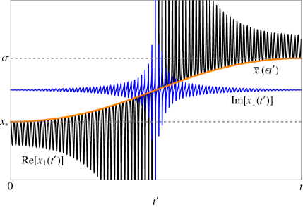
Figure 2: Upper panel: The complex-time contours on which the complex-time instanton $\phi_{1}$ and its Euclidean-time counterpart $\bar{\phi}$ are defined, where $z=(1-i\epsilon)t$. Lower panel: The real (black) and imaginary (blue) parts of a generic complex-time instanton $x_{1}$ for a point particle, together with the corresponding Euclidean-time instanton $\bar{x}$ (red). The real part of the complex-time instanton describes a driven oscillation within the false-vacuum basin, whose turning points between the regions $\mathcal{F}$ and $\mathcal{R}$ interpolate to the Euclidean-time instanton.

Vacuum decay in complex time. It is well-understood that the familiar Euclidean-time results for tunneling out of the false vacuum can be obtained from the description in real, physical time through a Wick rotation. This would imply in particular that the infinite Euclidean-time extent of the instanton is the result of an infinite (real-valued) physical time. For tunneling out of pure excited states, meanwhile, it is well-known that the relevant instantons are defined only over a Euclidean-time interval of finite length, which is fixed by the initial state, independent of the physical time [40, 41, 42, 43]. This suggests the need for a more careful treatment of the transition to imaginary time, as given in our companion paper Ref. [44].

The most important result of Ref. [44] can be anticipated through careful consideration of recent results for the decay rate out of the false vacuum given in Refs. [20, 26]. In complex time $z=(1-i\epsilon)t$, the instanton itself becomes a complex function [18, 19, 20, 21, 22, 23, 24, 26, 28]. The real part of these solutions can be understood as the particle oscillating in the false-vacuum basin, in the process sourcing an imaginary part through an interaction controlled by $\epsilon$. Its backreaction then further drives the oscillation of the real part until it ultimately leaves the false-vacuum basin, followed by a damping that causes the solution to converge to the desired final state. See Fig. 2. Most important, the dynamics arising from “interactions” between the real and imaginary parts is controlled by the change in $t\cdot\epsilon=-{\rm Im}(z)=\tau$. This suggests that the tunneling occurs once this combination has reached a certain fixed value. This observation is consistent with the perspective developed in Ref. [22], in which it is suggested that any complex-time process can be split into a Euclidean-time part, corresponding to quantum effects, and a real-time part, describing a classically allowed motion.

In Ref. [44], we demonstrate explicitly that this distinction can also be extended to the action itself. In the limit $t\to\infty$, the imaginary part of the action corresponding to the complex-time instanton solution converges to the Euclidean-time result with the same $\Delta{\rm Im}(z)$. In terms of the two complex-time contours represented in Fig. 3, this can be formalized through the statement

$$iS[\phi_{1}]-iS^{*}[\phi_{2}]\overset{t\to\infty}{\longrightarrow}S_{E}[\bar{\phi}],$$ (6)

where $\phi_{1}$ and $\phi_{2}$ are the periodic instantons in complex time on the upper and lower diagonal contours, respectively, and $\bar{\phi}$ is the conventional instanton, defined on the Euclidean-time interval. See Fig. 3. Whereas the origin of the latter is rather subtle for the case of a pure excited state, we find that working with a thermal ensemble naturally circumvents the underlying issues, as $\Delta{\rm Im}(z)$ is set by the temperature: $|\Delta{\rm Im}(z)|=\beta=T^{-1}$.

Figure 3: The exponent of the decay rate consists of contributions arising from the action of (complexified) instantons defined on two complex-time contours. In the limit of an infinitely long physical time, the sum of these contributions converges to the Euclidean action of the Euclidean-time instanton stretching over the same $\Delta{\rm Im}(z)$.

Evaluating the Decay Rate. We will evaluate Eq. (4) in two different ways. First, we show that it can be brought to a simple form that allows it to be understood as a superposition of the decay rates out of the individual states forming the thermal ensemble. Next we show that this result can equivalently be evaluated in terms of a periodic instanton, corresponding to a thermodynamical interpretation. Both of these results rely on the equivalence of complex-time decay-rate calculations with Euclidean-time results, which we establish in Ref. [44].

Microphysical picture. The probabilities on the right-hand side of Eq. (4) can be brought to a more convenient form with the insertion of two decompositions of unity:

$$\mathcal{P}_{\mathcal{R}}=\int D\varphi_{i}\int D\varphi_{j}\langle\varphi_{i}|\rho|\varphi_{j}\rangle\underset{\mathcal{R}}{\overset{}{\int}}D\varphi_{f}\langle\varphi_{j}|\varphi_{f},t\rangle\langle\varphi_{f},t|\varphi_{i}\rangle.$$ (7)

The first factor, $\rho_{ij}\equiv\langle\varphi_{i}|\rho|\varphi_{j}\rangle$, contains all information about the system of interest, while the second factor, $P_{ji}\equiv\int_{\mathcal{R}}D\varphi_{f}(...)$, is universal for all systems and reproduces the zero-temperature result in the limit $|\varphi_{j}\rangle\to|\varphi_{i}\rangle$. Here, as in the remainder of this article, all states without an explicit time label are to be understood as eigenstates of the field operator at $t=0$.

In analogy with the zero-temperature derivation presented in Refs. [7, 8], we begin by rewriting the transition amplitudes within $P_{ji}$. Making use of the fact that the states $|\varphi_{i,j}\rangle$ and $|\varphi_{f}\rangle$ lie in $\mathcal{F}$ and $\mathcal{R}$, respectively, we have

$$D_{F} (\varphi_{j}|\varphi_{f},t)\equiv\langle\varphi_{j},t_{j}|\varphi_{f},t_{f}\rangle=$$

$$=\int_{\smash[b]{\vphantom{\bigg{|}}}\Sigma_{\varphi_{j}}}D\sigma\int_{0}^{t}\text{d}s\ \bar{D}_{F}(\varphi_{j}|\sigma,s)D_{F}(\sigma,s|\varphi_{f},t).$$ (8)

To define the auxiliary quantity $\bar{D}_{F}$, we may first introduce the functional $T_{\varphi_{k}}[\varphi]$, which maps any time-dependent field configuration $\varphi$ onto the time when it first reaches the field-space hypersurface $\Sigma_{\varphi_{k}}\subset{\cal R}$, which contains all the configurations in ${\cal R}$ that have the same energy as $\varphi_{k}$. In terms of this object, $\bar{D}_{F}$ is defined as

$$\bar{D}_{F}(\varphi_{j}|\sigma,s)\equiv\underset{\varphi(0)=\varphi_{j}}{\overset{\varphi(s)=\sigma}{\int}}D\varphi\ e^{iS[\varphi]}\delta\left(T_{\varphi_{j}}[\varphi]-s\right).$$ (9)

We refer to $T_{\varphi_{j}}[\varphi]=s$ as the crossing condition.

The decomposition of Eq. (8) amounts to splitting the time evolution from $\varphi_{j}$ to $\varphi_{f}$ into a first piece connecting $\varphi_{j}$ with an energetically degenerate configuration in ${\cal R}$, and the time evolution thereafter. Using the same representation for $D_{F}(\varphi_{f},t|\varphi_{j})=D_{F}^{*}(\varphi_{j}|\varphi_{f},t)$, the combination $P_{ji}$ can be rewritten as

$$P_{ji}= \int_{\smash[b]{\vphantom{\bigg{|}}}\Sigma_{\varphi_{j}}}D\sigma\int_{0}^{t}\text{d}s\int_{\smash[b]{\vphantom{\bigg{|}}}\Sigma_{\varphi_{i}}}D\sigma^{\prime}\int_{0}^{t}\text{d}s^{\prime}\,\bar{D}_{F}(\varphi_{j}|\sigma,s)\bar{D}_{F}^{*}(\varphi_{i}|\sigma^{\prime},s^{\prime})$$

$$\times\int_{\smash[b]{\vphantom{\bigg{|}}}\cal R}D\varphi_{f}\,D_{F}(\sigma,s|\varphi_{f},t)D_{F}(\varphi_{f},t|\sigma^{\prime},s^{\prime}).$$ (10)

To further simplify this expression, we first restrict ourselves to a single tunneling event, i.e., we assume that no back-tunneling occurs. This allows us to approximate the path integral in the second line of Eq. (10) as $D_{F}(\sigma,s|\sigma^{\prime},s^{\prime})$. Next we rewrite the time integrals as

$$\int_{0}^{t}\text{d}s\int_{0}^{t}\text{d}s^{\prime}=\int_{0}^{t}\text{d}s\int_{0}^{s}\text{d}s^{\prime}+\int_{0}^{t}\text{d}s^{\prime}\int_{0}^{s^{\prime}}\text{d}s.$$ (11)

This allows us to recombine the propagator in Eq. (10) with one of the two factors of $\bar{D}_{F}$, using Eq. (8). Eliminating the remaining time integral by taking a derivative, we find

$$\frac{{\rm d}P_{ji}}{{\rm d}t}=\int_{\smash[b]{\vphantom{\bigg{|}}}\Sigma_{\varphi_{j}}}D\sigma\ \bar{D}_{F}(\varphi_{j}|\sigma,t)D_{F}^{*}(\sigma,t|\varphi_{i})+c.c.$$ (12)

Using the fact that $\rho_{ij}$, which describes the initial conditions, is time-independent, the decay rate can be represented through the path integral

$$\Gamma= \frac{1}{Z_{\beta}}\int D\varphi_{i}\int D\varphi_{j}\rho_{ij}\underset{\Sigma_{\varphi_{j}}}{\overset{}{\int}}D\sigma\bar{D}_{F}(\varphi_{j}|\sigma,t)D_{F}(\sigma,t|\varphi_{i})+c.c.$$ (13)

This expression, which is valid for any initial state, can be understood as the total decay rate consisting of the sum of the contributions from all states within $\mathcal{F}$, weighted by $\rho_{ij}$. For a thermal ensemble, it can be represented as a path integral,

$$\rho_{ij}=\underset{\varphi_{T}(0)=\varphi_{i}}{\overset{\varphi_{T}(\beta)=\varphi_{j}}{\int}}D\varphi_{T}\ e^{-S_{E}[\varphi_{T}]}.$$ (14)

The exponent of the integrand consists of three terms: two along the real-time axis, representing the tunneling, and one along the imaginary-time axis, representing the initial (thermal) probability distribution. Together with the integrals over their intersection points, this yields the well-known Schwinger-Keldysh contour. See Fig. 4.

An important subtlety in this picture is its reliance on contours defined on the real-time axis. As we previously pointed out, imposing the correct boundary conditions requires a minimal $\Delta\rm{Im}(z)$. This problem, however, is not linked to the thermal ensemble, but already appears for the case of a pure excited state. In Ref. [44], we point out that the interpretation of a real-time contour can be upheld if the regularization is assigned to the Hamiltonian, along the lines of Ref. [45]. Whereas this establishes a consistent way to define the decay rate as a Schwinger-Keldysh process, evaluating Eq. (13) still remains generally impractical due to the complexity of the saddle-point equations for arbitrary temperatures [37, 38].

Figure 4: The Keldysh-Schwinger contour arising from the microphysical picture.

Thermodynamical picture. In order to evaluate Eq. (4), we rewrite the probability of Eq. (3) by inserting a decomposition of unity in terms of field eigenstates and make the substitution $\beta=\beta_{1}+\beta_{2}$,

$$\mathcal{P}_{\mathcal{R}} =\mathcal{N}\int_{\mathcal{R}}D\varphi\langle\varphi|e^{iHt}\rho e^{-iHt}|\varphi\rangle=$$ (15)

$$= \mathcal{N}\underset{\mathcal{F}}{\overset{\ }{\int}}D\varphi_{*}\underset{\mathcal{F}}{\overset{\ }{\int}}D\varphi\langle\varphi|e^{iHt\left(1+i\frac{\beta_{1}}{t}\right)}|\varphi_{*}\rangle\langle\varphi_{*}|e^{-iHt\left(1-i\frac{\beta_{2}}{t}\right)}|\varphi\rangle.$$

In the limit of large physical times, the temperature-dependent term acts as a regulator of the time evolution operators, $\epsilon_{1,2}=\beta_{1,2}/t$. In terms of complex-time contours, this amounts to picking two paths with $\Delta\tau_{1,2}=\beta_{1,2}$, see Fig. 3. For $\beta_{1}=\beta_{2}$, the contribution of each $\varphi_{*}$ can be identified with the decay rate out of the corresponding eigenstate, up to the difference in the normalization factor $Z_{\beta}$. It is thus straightforward to adjust the derivation presented in Refs. [7, 8], leading to

$$\Gamma= \frac{1}{Z_{\beta}}\int D\varphi_{*}\underset{\Sigma_{\varphi_{j}}}{\overset{}{\int}}D\sigma\ \bar{D}_{F}^{\epsilon_{1}}(\varphi_{*}|\sigma,t)D_{F}^{\epsilon_{2}}(\sigma,t|\varphi_{*})+c.c.=$$

$$= \frac{1}{Z_{\beta}}\int D\varphi_{*}\underset{\Sigma_{\varphi_{*}}}{\overset{\ }{\int}}D\sigma\underset{\varphi_{1}(0)=\varphi_{*}}{\overset{\varphi_{1}(t)=\sigma}{\int}}D\varphi_{1}\ e^{iS_{\epsilon_{1}}[\varphi_{1}]}\delta\left(T_{\sigma}[\varphi_{1}]-t\right)$$

$$\times\left(\hskip 11.99998pt\underset{\varphi_{2}(0)=\varphi_{*}}{\overset{\varphi_{2}(t)=\sigma}{\int}}D\varphi_{2}\ e^{iS_{\epsilon_{2}}[\varphi_{2}]}\right)^{*}+c.c.$$ (16)

Here, all quantities with a label $\epsilon_{1,2}$ are to be understood as regularized using the parameter $\epsilon_{1,2}=\beta_{1,2}/t$.

Eq. (16) can be evaluated through a saddle-point approximation in the usual way. First, the normalization factor $Z_{\beta}$ is dominated by the constant saddle point $\phi_{\rm FV}$, leading to a vanishing exponent. To leading order, it is determined by solutions $\phi_{1,2}$ of the equations of motion along the real-time contours shown in Fig. 3. The integrals over the boundary values $\varphi_{*}$ and $\sigma$, meanwhile, pick a solution with the expected periodic boundary conditions along the ${\rm Im}(z)$ axis. Refs. [40, 41, 42, 43] provide a discussion of the properties of such solutions for tunneling out of the false vacuum, which we extend to more general cases in our companion article [44]. In general, these solutions give rise to a complex action. In the limit $t\to\infty$, these can be related to the action of a Euclidean-time instanton through Eq. (6),

$$\Gamma=\frac{A}{Z_{\beta}}e^{iS[\phi_{1}]-iS^{*}[\phi_{2}]}\overset{t\to\infty}{\longrightarrow}B\cdot e^{-S_{E}[\bar{\phi}]},$$ (17)

where the prefactor $B$ contains the usual loop-corrections linked to fluctuations around both the instanton and the constant saddle point in the denominator.

The coefficient $B$ also contains a factor $1/\beta$ arising from the decay rate’s invariance under translation along the Euclidean-time direction, which equivalently can be understood as a redundancy linked to the freedom to decompose $\beta$ into $\beta_{1}$ and $\beta_{2}$. See Fig. 5. For field-theoretic problems $B$ furthermore contains a factor proportional to the volume of space.

Figure 5: The periodic Euclidean-time instanton that determines the decay rate in the limit $t\to\infty$ for a point particle in a symmetric potential $V(x)$. The light-gray arrows indicate the periodic motion of the system within the inverted potential $-V(x)$. The saddle-point values of $x_{*}$ and $\sigma$, necessary for the existence of a solution, depend on the partition of $\beta$ into $\beta_{1}$ and $\beta_{2}$. For the special case $\beta_{1}=\beta_{2}$ the instanton mimics that for the decay out of the excited state $x_{*}$, corresponding to the turning point.

To better understand the analogy between the tunneling rate in the thermodynamical picture and for a pure, excited state, we may first note that the Euclidean action of any periodic instanton with period $\beta$ satisfies $S_{E}=E\beta+W$, where $E$ is the energy of the initial state and $W$ is the usual WKB exponent [43]. For the thermal ensemble, where $Z_{\beta}$ is dominated to leading order by the contribution from the constant saddle point with $S_{E}=0$, this result has a simple interpretation as the superposition of a thermal suppression (first term) and a tunneling suppression (second term).

The crucial difference between this result and that for the tunneling rate out of a pure excited state is the dominant saddle point in the normalization factor $Z$. As the constant solution is not consistent with the boundary conditions arising from a pure state, it is instead dominated by a non-constant solution with $S_{E}\simeq E\beta$ [44]. Thus, the apparent thermal suppression cancels to leading order, leaving only the desired tunneling term.

Multifield Models and the Effective Action. In many real-world applications, including the stability of the Higgs vacuum in the Standard Model (SM), one has to take into account the effects of external degrees of freedom, which affect the tunneling only through interactions. We can incorporate them into our definition of the tunneling process by extending the trace as

$$\mathcal{P}_{\mathcal{R}}(t)=\mathcal{N}\int D\chi\int_{\mathcal{R}}D\varphi\,\langle\varphi,\chi,t|\rho|\varphi,\chi,t\rangle.$$ (18)

This amounts to allowing for any configuration of the background fields $\chi$ after the tunneling. For the zero-temperature case, it was argued in Ref. [8] that the proper way to account for these additional path integrals is to first solve for the instanton using the tree-level potential and only afterwards integrate over the remaining fields, such that their effect is reduced to additional contributions to the prefactor $B$.

It is well-known that loop-corrections to the potential can be significant in finite-temperature systems, e.g., through particles obtaining thermal masses [46, 47, 48]. This suggests to integrate out the external fields before performing the saddle-point approximation in order to capture these effects, which would amount to working with an effective action. In Ref. [8], however, it was pointed out that the instanton background can spoil the convergence of momentum-dependent corrections to the effective action. Denoting the field giving rise to the instanton by $\phi$, these are suppressed by increasingly higher orders of $m_{\phi}^{2}/m_{i}^{2}$, where $m_{i}^{2}$ is the field-dependent mass of the particles being integrated out [48, 49, 50]. Hence, while the fluctuations of the field $\phi$ always need to be evaluated in their functional determinant form, any other field can be accounted for through its contributions to the effective action as long as its (effective) mass is larger than that of the scalar field around the instanton [51]. An important example for this scenario is thermally induced electroweak vacuum decay in the SM. Combining the scaling of the instanton, $\phi\sim|\lambda|^{-1/2}T$, with the inferred values of the relevant couplings at high energies, it is straightforward to find that all particles besides the Higgs itself and the Goldstone modes can be integrated out consistently.

Important Limits. In the limit of low temperatures our approach naturally reproduces the familiar zero-temperature results as $\beta\to\infty$. As the high-temperature limit corresponds to large occupation numbers, it can, in general be expected to yield the classical limit [29, 30, 31, 32, 33, 34, 35, 36], in which the exponent is to leading order determined by a constant solution in the Euclidean-time direction.

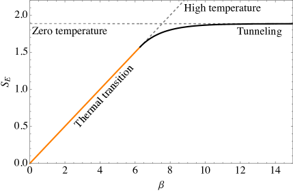
Figure 6: The Euclidean action as a function of inverse temperature $\beta$ for the potential $V(x)=\frac{1}{4}(x^{2}-1)^{2}$. We find a smooth limit for both high and low temperatures. Quantum tunneling is only relevant for $\beta\gtrsim 6.28$ in these units, which corresponds to the oscillator period for motions around the minimum of the inverted potential. For smaller values of $\beta$, the transition is entirely determined by thermal excitations.

For a point particle, the instanton can be represented as a periodic motion in the inverse potential, see Fig. 5. It is easy to see that, for a generic potential, the Euclidean time necessary for such motions is bounded from below by some $\Delta\tau_{\rm min}$ that scales with the mass scale of the potential. Hence, for smaller values of $\beta$ no periodic solution exists, leaving only the saddle point corresponding to the particle being at rest on top of the potential barrier, $\phi=\phi_{\rm top}$. It is worth noting that this configuration on its own violates the crossing condition. This changes, however, once fluctuations around it are taken into account, as the path integral over all configurations also covers a non-vanishing subset for which $\delta\phi<0$ until the crossing time.

The transition between the instanton-dominated regime to the sphaleron-dominated regime is easily understood through the relation $S_{E}=\beta E+W$. For a generic potential, the smallest possible value of $\beta$ corresponds to infinitesimally small oscillations around $\phi_{\rm top}$. This implies immediately that in this limit $W\to 0$ and $E\to E[\phi_{\rm top}]$, suggesting a smooth limit. The properties of this limit are investigated in more detail in Ref. [52].

An important subtlety is that this limit can be prevented by background-field effects. Integrating out heavy degrees of freedom at a finite temperature induces temperature-dependent corrections to the potential, including a mass term. For temperatures significantly larger than the tree-level mass, the magnitude of these terms is controlled by the temperature alone. As an example, the thermal mass is generally of the form $m_{T}^{2}=\kappa\cdot T^{2}$, with some combination of the scalar field’s couplings to the background fields $\kappa$, but, importantly, no additional loop-suppression factor $(4\pi)^{-2N_{\rm loop}}$. In other words, all relevant energy scales of the theory are of order of the temperature up to numerical coefficients, which can be ${\cal O}(1)$ for sufficiently large couplings. This can be understood as the energy per particle increasing due to its coupling to an increasingly hot background plasma counteracting the increase in the occupation number. An important example for this behavior is the SM Higgs field, for which we find that the coefficient $\kappa$ lies within the range $0.1-0.2$ for all energies above the central value of the instability scale, $\mu_{I}\sim 10^{11}$ GeV [53]. While this establishes in principle the possibility of a perturbative expansion, it also suggests that precision calculations should take into account leading-order corrections in $\kappa$, in particular since the effects of, e.g., potentially large right-handed neutrinos can further enhance this effect [12].

Discussion. We have derived compact path-integral representations for the tunneling rate for an arbitrary finite-temperature system. Unlike previous treatments, which have often relied on analogies, our first-principles derivation clarifies several conceptual questions. In particular, we have shown that the finite-temperature decay rate can indeed be understood as a superposition of contributions from each state in the thermal ensemble. This expression can be rewritten in a way that allows one to perform a combined saddle-point approximation. The properties of the resulting complex-time instanton imply that, in the limit of large physical times, the exponent of the decay rate converges to the Euclidean action of the familiar Euclidean-time instanton with period $\beta$.

This simple relation explains how the decay rate, which is a priori a real-time-dependent quantity, can be described in terms of a Euclidean-time quantity. This result can be understood as the tunneling being dominated by the contribution of one state in the thermal ensemble. In addition, we have analyzed the influence of background fields on the decay rate as well as subtleties related to both the high- and low-temperature limits. This establishes a robust foundation for tunneling and bubble-nucleation calculations at arbitrary temperatures.

Acknowledgements. TS’s contributions to this work were made possible by the Walter Benjamin Programme of the Deutsche Forschungsgemeinschaft (DFG, German Research Foundation) – 512630918. MK is supported in part by the MLK Visiting Scholars Program at MIT. Portions of this work were conducted in MIT’s Center for Theoretical Physics and partially supported by the U.S. Department of Energy under Contract No. DE-SC0012567. This project was also supported in part by the Black Hole Initiative at Harvard University, with support from the Gordon and Betty Moore Foundation and the John Templeton Foundation. The opinions expressed in this publication are those of the author(s) and do not necessarily reflect the views of these Foundations.

References

- Kobzarev et al. [1974] I. Y. Kobzarev, L. B. Okun, and M. B. Voloshin, Bubbles in Metastable Vacuum, Yad. Fiz. 20, 1229 (1974).
- Coleman [1977] S. R. Coleman, The Fate of the False Vacuum. 1. Semiclassical Theory, Phys. Rev. D 15, 2929 (1977), [Erratum: Phys.Rev.D 16, 1248 (1977)].
- Callan and Coleman [1977] C. G. Callan, Jr. and S. R. Coleman, The Fate of the False Vacuum. 2. First Quantum Corrections, Phys. Rev. D 16, 1762 (1977).
- Devoto et al. [2022] F. Devoto, S. Devoto, L. Di Luzio, and G. Ridolfi, False vacuum decay: an introductory review, J. Phys. G 49, 103001 (2022), arXiv:2205.03140 [hep-ph] .
- Linde [1981] A. D. Linde, Fate of the False Vacuum at Finite Temperature: Theory and Applications, Phys. Lett. B 100, 37 (1981).
- Linde [1983] A. D. Linde, Decay of the False Vacuum at Finite Temperature, Nucl. Phys. B 216, 421 (1983), [Erratum: Nucl.Phys.B 223, 544 (1983)].
- Andreassen et al. [2016] A. Andreassen, D. Farhi, W. Frost, and M. D. Schwartz, Direct Approach to Quantum Tunneling, Phys. Rev. Lett. 117, 231601 (2016), arXiv:1602.01102 [hep-th] .
- Andreassen et al. [2017] A. Andreassen, D. Farhi, W. Frost, and M. D. Schwartz, Precision decay rate calculations in quantum field theory, Phys. Rev. D 95, 085011 (2017), arXiv:1604.06090 [hep-th] .
- Andreassen et al. [2018] A. Andreassen, W. Frost, and M. D. Schwartz, Scale Invariant Instantons and the Complete Lifetime of the Standard Model, Phys. Rev. D 97, 056006 (2018), arXiv:1707.08124 [hep-ph] .
- Khoury and Steingasser [2022] J. Khoury and T. Steingasser, Gauge hierarchy from electroweak vacuum metastability, Phys. Rev. D 105, 055031 (2022), arXiv:2108.09315 [hep-ph] .
- Steingasser [2022] T. Steingasser, New perspectives on solitons and instantons in the Standard Model and beyond, Ph.D. thesis, Munich U. (2022).
- Chauhan and Steingasser [2023] G. Chauhan and T. Steingasser, Gravity-improved metastability bounds for the Type-I seesaw mechanism, JHEP 09, 151, arXiv:2304.08542 [hep-ph] .
- Espinosa [2018] J. R. Espinosa, A Fresh Look at the Calculation of Tunneling Actions, JCAP 07, 036, arXiv:1805.03680 [hep-th] .
- Espinosa [2019a] J. R. Espinosa, Fresh look at the calculation of tunneling actions including gravitational effects, Phys. Rev. D 100, 104007 (2019a), arXiv:1808.00420 [hep-th] .
- Espinosa and Konstandin [2019] J. R. Espinosa and T. Konstandin, A Fresh Look at the Calculation of Tunneling Actions in Multi-Field Potentials, JCAP 01, 051, arXiv:1811.09185 [hep-th] .
- Espinosa [2019b] J. R. Espinosa, Tunneling without Bounce, Phys. Rev. D 100, 105002 (2019b), arXiv:1908.01730 [hep-th] .
- Espinosa et al. [2023] J. R. Espinosa, R. Jinno, and T. Konstandin, Tunneling potential actions from canonical transformations, JCAP 02, 021, arXiv:2209.03293 [hep-th] .
- Witten [2011] E. Witten, Analytic Continuation Of Chern-Simons Theory, AMS/IP Stud. Adv. Math. 50, 347 (2011), arXiv:1001.2933 [hep-th] .
- Tanizaki and Koike [2014] Y. Tanizaki and T. Koike, Real-time Feynman path integral with Picard–Lefschetz theory and its applications to quantum tunneling, Annals Phys. 351, 250 (2014), arXiv:1406.2386 [math-ph] .
- Cherman and Unsal [2014] A. Cherman and M. Unsal, Real-Time Feynman Path Integral Realization of Instantons, (2014), arXiv:1408.0012 [hep-th] .
- Dunne and Ünsal [2016] G. V. Dunne and M. Ünsal, What is QFT? Resurgent trans-series, Lefschetz thimbles, and new exact saddles, PoS LATTICE2015, 010 (2016), arXiv:1511.05977 [hep-lat] .
- Bramberger et al. [2016] S. F. Bramberger, G. Lavrelashvili, and J.-L. Lehners, Quantum tunneling from paths in complex time, Phys. Rev. D 94, 064032 (2016), arXiv:1605.02751 [hep-th] .
- Michel [2020] F. Michel, Parametrized Path Approach to Vacuum Decay, Phys. Rev. D 101, 045021 (2020), arXiv:1911.12765 [quant-ph] .
- Mou et al. [2019] Z.-G. Mou, P. M. Saffin, and A. Tranberg, Quantum tunnelling, real-time dynamics and Picard-Lefschetz thimbles, JHEP 11, 135, arXiv:1909.02488 [hep-th] .
- Hertzberg and Yamada [2019] M. P. Hertzberg and M. Yamada, Vacuum Decay in Real Time and Imaginary Time Formalisms, Phys. Rev. D 100, 016011 (2019), arXiv:1904.08565 [hep-th] .
- Ai et al. [2019] W.-Y. Ai, B. Garbrecht, and C. Tamarit, Functional methods for false vacuum decay in real time, JHEP 12, 095, arXiv:1905.04236 [hep-th] .
- Hayashi et al. [2022] T. Hayashi, K. Kamada, N. Oshita, and J. Yokoyama, Vacuum decay in the Lorentzian path integral, JCAP 05 (05), 041, arXiv:2112.09284 [hep-th] .
- Nishimura et al. [2023] J. Nishimura, K. Sakai, and A. Yosprakob, A new picture of quantum tunneling in the real-time path integral from Lefschetz thimble calculations, JHEP 09, 110, arXiv:2307.11199 [hep-th] .
- Langer [1967] J. S. Langer, Theory of the condensation point, Annals Phys. 41, 108 (1967).
- Langer [1969] J. S. Langer, Statistical theory of the decay of metastable states, Annals Phys. 54, 258 (1969).
- Bochkarev and de Forcrand [1993] A. Bochkarev and P. de Forcrand, Nonperturbative evaluation of the diffusion rate in field theory at high temperatures, Phys. Rev. D 47, 3476 (1993), arXiv:hep-lat/9210027 .
- Boyanovsky and Aragao de Carvalho [1993] D. Boyanovsky and C. Aragao de Carvalho, Real time analysis of thermal activation via sphaleron transitions, Phys. Rev. D 48, 5850 (1993), arXiv:hep-ph/9306238 .
- Garny and Konstandin [2012] M. Garny and T. Konstandin, On the gauge dependence of vacuum transitions at finite temperature, JHEP 07, 189, arXiv:1205.3392 [hep-ph] .
- Ekstedt [2022] A. Ekstedt, Bubble nucleation to all orders, JHEP 08, 115, arXiv:2201.07331 [hep-ph] .
- Hirvonen et al. [2022] J. Hirvonen, J. Löfgren, M. J. Ramsey-Musolf, P. Schicho, and T. V. I. Tenkanen, Computing the gauge-invariant bubble nucleation rate in finite temperature effective field theory, JHEP 07, 135, arXiv:2112.08912 [hep-ph] .
- Löfgren et al. [2023] J. Löfgren, M. J. Ramsey-Musolf, P. Schicho, and T. V. I. Tenkanen, Nucleation at Finite Temperature: A Gauge-Invariant Perturbative Framework, Phys. Rev. Lett. 130, 251801 (2023), arXiv:2112.05472 [hep-ph] .
- Affleck [1981] I. Affleck, Quantum Statistical Metastability, Phys. Rev. Lett. 46, 388 (1981).
- Lapedes and Mottola [1982] A. Lapedes and E. Mottola, Complex Path Integrals and Finite Temperature, Nucl. Phys. B 203, 58 (1982).
- Shkerin and Sibiryakov [2021] A. Shkerin and S. Sibiryakov, Black hole induced false vacuum decay from first principles, JHEP 11, 197, arXiv:2105.09331 [hep-th] .
- Liang et al. [1992] J.-Q. Liang, H. J. W. Muller-Kirsten, and D. H. Tchrakian, Solitons, bounces and sphalerons on a circle, Phys. Lett. B 282, 105 (1992).
- Liang and Muller-Kirsten [1992] J.-Q. Liang and H. J. W. Muller-Kirsten, Periodic instantons and quantum mechanical tunneling at high-energy, Phys. Rev. D 46, 4685 (1992).
- Liang and Mueller-Kirsten [1994] J. Q. Liang and H. J. W. Mueller-Kirsten, Quantum mechanical tunneling at finite energy and its equivalent amplitudes in the (vacuum) instanton approximation, Phys. Lett. B 332, 129 (1994).
- Liang and Muller-Kirsten [1994] J. Q. Liang and H. J. W. Muller-Kirsten, Nonvacuum bounces and quantum tunneling at finite energy, Phys. Rev. D 50, 6519 (1994).
- [44] T. Steingasser and D. I. Kaiser, Complex time and quantum tunneling from arbitrary initial states, in prep .
- Kaya [2019] A. Kaya, On Prescription in Cosmology, JCAP 04, 002, arXiv:1810.12324 [gr-qc] .
- Carrington [1992] M. E. Carrington, The Effective potential at finite temperature in the Standard Model, Phys. Rev. D 45, 2933 (1992).
- Kajantie et al. [1996] K. Kajantie, M. Laine, K. Rummukainen, and M. E. Shaposhnikov, Generic rules for high temperature dimensional reduction and their application to the standard model, Nucl. Phys. B 458, 90 (1996), arXiv:hep-ph/9508379 .
- Salvio et al. [2016] A. Salvio, A. Strumia, N. Tetradis, and A. Urbano, On gravitational and thermal corrections to vacuum decay, JHEP 09, 054, arXiv:1608.02555 [hep-ph] .
- Moss et al. [1992] I. G. Moss, D. J. Toms, and W. A. Wright, The Effective Action at Finite Temperature, Phys. Rev. D 46, 1671 (1992).
- Bodeker et al. [1994] D. Bodeker, W. Buchmuller, Z. Fodor, and T. Helbig, Aspects of the cosmological electroweak phase transition, Nucl. Phys. B 423, 171 (1994), arXiv:hep-ph/9311346 .
- Gleiser et al. [1993] M. Gleiser, G. C. Marques, and R. O. Ramos, On the evaluation of thermal corrections to false vacuum decay rates, Phys. Rev. D 48, 1571 (1993), arXiv:hep-ph/9304234 .
- Chudnovsky [1992] E. M. Chudnovsky, Phase transitions in the problem of the decay of a metastable state, Phys. Rev. A 46, 8011 (1992).
- Steingasser and Kaiser [2023] T. Steingasser and D. I. Kaiser, Higgs Criticality beyond the Standard Model, (2023), arXiv:2307.10361 [hep-ph] .