A nonlinear spectral core-periphery detection method for multiplex networks

Abstract

Core-periphery detection aims to separate the nodes of a complex network into two subsets: a core that is densely connected to the entire network and a periphery that is densely connected to the core but sparsely connected internally. The definition of core-periphery structure in multiplex networks that record different types of interactions between the same set of nodes but on different layers is nontrivial since a node may belong to the core in some layers and to the periphery in others. The current state-of-the-art approach relies on linear combinations of individual layer degree vectors whose layer weights need to be chosen a-priori. We propose a nonlinear spectral method for multiplex networks that simultaneously optimizes a node and a layer coreness vector by maximizing a suitable nonconvex homogeneous objective function by an alternating fixed point iteration. We prove global optimality and convergence guarantees for admissible hyper-parameter choices and convergence to local optima for the remaining cases. We derive a quantitative measure for the quality of a given multiplex core-periphery structure that allows the determination of the optimal core size. Numerical experiments on synthetic and real-world networks illustrate that our approach is robust against noisy layers and outperforms baseline methods with respect to a variety of core-periphery quality measures. In particular, all methods based on layer aggregation are improved when used in combination with the novel optimized layer coreness vector weights. As the runtime of our method depends linearly on the number of edges of the network it is scalable to large-scale multiplex networks.

05C50, 05C82, 47H09, 47J26, 65H17, 91C20

1 Introduction

Complex networked systems are all around us: interactions of users, items, stops, genes, proteins, or machines can all be recorded by pairwise connections [39, 21]. In recent years, multilayer networks in which different types of interactions are represented in different layers have gained increased attention [32, 7]. Consequently, several quantitative means for the structural analysis of complex networks such as community detection [37, 36, 4] or centrality analysis [20, 45, 3] have been generalized from single- to multi-layered networks. In this work, we focus on node-aligned multiplex networks without inter-layer edges.

Core-periphery structure is a mesoscopic network property combining the concepts of community structure and centrality as it seeks to partition a network’s node set into a set of core and a set of periphery nodes. Core nodes are characterized by a high degree of connectivity to the full network while periphery nodes may be strongly connected to the core but are sparsely connected to other peripheral nodes. Common synonyms are rich-club [14] and core-fringe structure [2]. The seminal work by Borgatti and Everett formalized an ideal core-periphery structure as an L-shaped block adjacency matrix in which core nodes are connected to all other nodes but no edges are present between pairs of periphery nodes [8]. This binary partitioning problem of nodes into two sets, however, leads to combinatorial optimization problems that are computationally prohibitive to solve exactly even for relatively small networks. Instead, a number of approaches for the approximate solution exist in the literature, some of which heavily rely on centrality measures, cf. e.g., [8, 29, 9, 31, 10, 15, 41, 48, 16, 35, 30, 22]. Existing approaches for core-periphery detection in single-layer networks typically rely on maximizing an objective function

(1) $$f(\bm{x})=\sum_{i,j=1}^{n}\bm{A}_{ij}\kappa(\bm{x}_{i},\bm{x}_{j})$$

for a node coreness vector $\bm{x}\in\mathbb{R}^{n}_{\geq 0}$, with large entries for nodes belonging to the core. Here, $\bm{A}_{ij}\geq 0$ denotes the edge weight between nodes $i$ and $j$ with $i,j=1,\dots,n$ and $\kappa:\mathbb{R}_{\geq 0}\times\mathbb{R}_{\geq 0}\rightarrow\mathbb{R}_{\geq 0}$ a kernel function. A commonly chosen kernel function is the maximum kernel $\kappa(\bm{x}_{i},\bm{x}_{j})=\max\{\bm{x}_{i},\bm{x}_{j}\}$, which relates to the ideal L-shape model in the sense that $\bm{A}_{ij}$ contributes to Eq. 1 if at least one of the nodes $i$ or $j$ belongs to the core.

More recently, the logistic core-periphery random graph model has been introduced as a relaxed version of the ideal L-shape model of core-periphery structure [46, 30]. It motivates the usage of a smoothed maximum function

(2) $$\kappa(\bm{x}_{i},\bm{x}_{j})=\left(\bm{x}_{i}^{\alpha}+\bm{x}_{j}^{\alpha}\right)^{1/\alpha}\underset{\alpha\rightarrow\infty}{\longrightarrow}\max\{\bm{x}_{i},\bm{x}_{j}\}$$

as kernel function for vectors $\bm{x}\in\mathbb{R}^{n}_{>0}$ [46]. Recent advances in nonlinear Perron–Frobenius theory guarantee the unique solvability of the non-convex constrained optimization problem of maximizing Eq. 1 subject to norm constraints on $\bm{x}$ by means of a nonlinear power iteration [45, 46, 25].

The formulation of core-periphery structure in multilayer networks is still in its infancy. In multiplex networks, each entity is represented by one node in each layer and the definition of multiplex coreness is non-trivial since, in general, each layer may possess a different core-periphery structure or none at all. The most prominent approach to date utilizes linear combinations

(3) $$\bm{x}=\bm{c}_{1}\bm{d}^{(1)}+\cdots+\bm{c}_{L}\bm{d}^{(L)}$$

of the node degree vectors $\bm{d}^{(1)},\dots,\bm{d}^{(L)}\in\mathbb{R}^{n}_{\geq 0}$ of the $L$ layers of the multiplex network weighted by a layer coreness vector $\bm{c}\in\mathbb{R}^{L}_{\geq 0}$ with $\|\bm{c}\|_{1}=1$, which needs to be chosen a-priori [1]. In the absence of expert knowledge suggesting otherwise, the authors propose the choice of equal layer weights, i.e., layer coreness vectors $\bm{c}=\frac{1}{L}\bm{1}$ with $\bm{1}\in\mathbb{R}^{L}$ the vector of all ones and results of experiments for other choices of $\bm{c}$ are presented. Furthermore, a recent extension of Eq. 3 additionally takes inter-layer connections, i.e., edges across layers into account and the influence of different layer weight vectors $\bm{c}$ is studied experimentally [33].

In this work, we formulate an objective function $f_{\alpha}(\bm{x},\bm{c})$ for core-periphery detection in multiplex networks that simultaneously optimizes a node and a layer coreness vector $\bm{x}\in\mathbb{R}^{n}_{>0}$ and $\bm{c}\in\mathbb{R}^{L}_{>0}$, respectively. It is based on the smoothed maximum kernel function Eq. 2 and can be seen as a generalization of the nonlinear spectral core-periphery detection method for single-layer networks [46]. We show that under suitable conditions, the unique maximum of $f_{\alpha}(\bm{x},\bm{c})$ can be computed by an alternating nonlinear power iteration summarized in Algorithm 1. Furthermore, we prove convergence of $f_{\alpha}(\bm{x},\bm{c})$ to a local maximum in cases in which the assumptions for unique solvability are not satisfied. We present different quantitative indicators for the quality of a given multiplex core-periphery partition and derive optimal core sizes.

We perform extensive numerical experiments on two types of multiplex networks: single-layer networks with strong core-periphery structure with a second random noise layer as well as real-world multiplex networks with an unknown distribution of core-periphery structure across the layers. The results indicate that our proposed method outperforms the multilayer degree method [1] in all but one experiment while improving the latter with the novel optimized layer coreness weights. Additionally, we distinctly outperform existing single-layer methods applied to aggregated versions of the multiplex networks. Experiments on the first type of networks illustrate that our approach allows the automated detection of noise layers, which is widely acknowledged to be a difficult yet highly relevant problem in multilayer network science [47, 40, 13, 36]. As the runtime of our method depends linearly on the number of edges in the network, Algorithm 1 is scalable to large-scale multiplex networks.

The remainder of this paper is structured as follows. Section 2 formulates the multiplex core-periphery detection problem. We propose our nonlinear spectral method for multiplex networks in Section 3 and prove convergence guarantees to global and local optima in different parameter settings. In Section 4, we summarize our algorithm before Section 5 discusses the determination of optimal core sizes and the quality of multiplex core-periphery partitions. Finally, Section 6 reports numerical experiments on artificial and real-world multiplex networks.

2 Problem formulation

We consider connected, binary, and undirected multiplex networks without self-edges and inter-layer edges and choose a third-order adjacency tensor representation

$$\bm{A}\in\mathbb{R}^{n\times n\times L},\quad\text{with}\quad\left[\bm{A}_{ij}^{(k)}\right]_{i,j=1,\dots,n}^{k=1,\dots,L},$$

where $n\in\mathbb{N}$ denotes the number of nodes and $L\in\mathbb{N}$ the number of layers, i.e., the $n\times n$ adjacency matrix of layer $k$ is found in the $k$-th frontal slice of $\bm{A}$. Hence, we have

$$\bm{A}_{ij}^{(k)}=\begin{cases}1&\text{if nodes }i\text{ and }j\text{ with }i\neq j\text{ are connected on layer }k,\\ 0&\text{otherwise,}\end{cases}$$

as well as $\bm{A}_{ij}^{(k)}=\bm{A}_{ji}^{(k)}$ for $i,j=1,\dots,n$ and $k=1,\dots,L$.

We seek a partition of the network’s nodes into a set of core and a set of periphery nodes. However, each node is represented in every layer and may belong to the core in some layers and to the periphery in others. To combine the coreness information from different layers by a layer coreness vector $\bm{c}\in\mathbb{R}^{L}_{>0}$, we adapt the approach from [1] of considering linear combinations Eq. 3. In the multilayer degree approach of [1], the coreness vector of the nodes is computed as $\bm{c}_{1}\bm{d}^{(1)}+\cdots+\bm{c}_{L}\bm{d}^{(L)}$, where $\bm{d}^{(k)}$ is the degree vector of the layer $k$, and $\bm{c}$ is a layer-weighting vector that must be chosen a-priori. Note that, due to the linearity of the degree, this vector coincides with the degree vector of the aggregated multiplex network with adjacency matrix $\sum_{k=1}^{L}\bm{c}_{k}\bm{A}_{ij}^{(k)}$. Leveraging this second interpretation, we propose a multiplex core-periphery objective function that simultaneously optimizes the node score and the layers’ weights $\bm{c}$.

Due to its success in the single-layer case, we adopt the logistic core-periphery objective function [46, 30] and propose an extension of the corresponding nonlinear spectral method. Our multiplex objective function reads

(4) $$f_{\alpha}(\bm{x},\bm{c})=\sum_{k=1}^{L}\sum_{i,j=1}^{n}\bm{c}_{k}\bm{A}_{ij}^{(k)}(\bm{x}_{i}^{\alpha}+\bm{x}_{j}^{\alpha})^{1/\alpha},$$

which we want to maximize simultaneously with respect to $\bm{x}\in\mathbb{R}^{n}_{>0}$, the (common) node coreness vector across the layers, and $\bm{c}\in\mathbb{R}^{L}_{>0}$, the layer coreness weights vector. Due to Eq. 2, when $\alpha$ is large enough, $f_{\alpha}$ takes large values each time that an edge exists $\bm{A}_{ij}^{(k)}\neq 0$ on a layer with large core score $\bm{c}_{k}$, at least one of the two nodes $i,j$ is in the core, i.e. either $\bm{x}_{i}$ or $\bm{x}_{j}$ is large.

To avoid trivial solutions (with all the entries blowing up to infinity), we require norm constraints on the vectors $\bm{x}$ and $\bm{c}$. This is not a limitation as we are ultimately seeking a relative score for both nodes and layers. Thus, we restrict $\bm{x}$ to $\mathcal{S}_{p}^{+}=\{\bm{x}\in\mathbb{R}^{n}_{>0}\colon\|\bm{x}\|_{p}=1\}$ and $\bm{c}$ to $\mathcal{S}_{q}^{+}=\{\bm{c}\in\mathbb{R}^{L}_{>0}\colon\|\bm{c}\|_{q}=1\}$. We will discuss the roles of $p,q>1$ in Section 3. Overall, our nonlinear spectral method for core-periphery detection in multiplex networks relies on the solution of the problem

(5) $$\max_{\bm{x}\in\mathcal{S}_{p}^{+},\bm{c}\in\mathcal{S}_{q}^{+}}~{}f_{\alpha}(\bm{x},\bm{c}).$$

Note that $f_{\alpha}(\bm{x},\bm{c})$ is 1-homogeneous in both $\bm{x}$ and $\bm{c}$ independently, i.e., we have $f_{\alpha}(\beta\bm{x},\bm{c})=f_{\alpha}(\bm{x},\beta\bm{c})=\beta f_{\alpha}(\bm{x},\bm{c})$ for all $\beta\in\mathbb{R}$, which we denote by $f_{\alpha}(\bm{x},\cdot)\in\text{hom}(1)$ and $f_{\alpha}(\cdot,\bm{c})\in\text{hom}(1)$. This shows that the restriction of $\bm{x}$ to $\mathcal{S}_{p}^{+}$ and of $\bm{c}$ to $\mathcal{S}_{q}^{+}$ can be generalized to vectors of arbitrary norms.

By [46, Lemma 4.2] and the 1-homogeneity of $f_{\alpha}(\bm{x},\bm{c})$ in both $\bm{x}$ and $\bm{c}$, we can reformulate Eq. 5 as the equivalent unconstrained optimization problem

(6) $$\max_{\bm{x}\in\mathbb{R}^{n}_{>0},\bm{c}\in\mathbb{R}^{L}_{>0}}~{}g_{\alpha}(\bm{x},\bm{c})\qquad\text{with}\qquad g_{\alpha}(\bm{x},\bm{c})=\frac{f_{\alpha}(\bm{x},\bm{c})}{\|\bm{x}\|_{p}\|\bm{c}\|_{q}}\,.$$

Note that for the special case of one layer, i.e., $L=1$ and $\bm{c}=1$, we recover the logistic core-periphery model for single-layer networks as proposed in [46].

3 Nonlinear spectral method for multiplex networks

The single-layer nonlinear spectral method [46] computes the solution of the constrained nonconvex optimization problem

$$\max_{\bm{x}\in\mathcal{S}_{p}^{+}}f(\bm{x})=\sum_{i,j=1}^{n}\bm{A}_{ij}(\bm{x}_{i}^{\alpha}+\bm{x}_{j}^{\alpha})^{1/\alpha},$$

for $\bm{A}\in\mathbb{R}_{\geq 0}^{n\times n}$ the single-layer adjacency matrix, by means of a provably globally convergent fixed point iteration. In this section, we introduce a nonlinear spectral method for multiplex networks by generalizing the single-layer results to the multivariate constrained nonconvex optimization problem Eq. 5 and proving convergence to a unique maximum by the bi-level optimization procedure summarized in Algorithm 1. Furthermore, we propose a second generalization of the single-layer nonlinear spectral method by proving convergence to local maxima for any parameters $p,q>1$ that do not necessarily permit unique solvability. Numerical experiments indicate that solutions with relatively small parameters $p$ and $q$ often yield better core-periphery partitions for single-layer and multiplex networks in terms of different metrics, which are introduced in Section 5.

Throughout this paper, we denote the gradient of the $p$-norm by $J_{p}(\bm{x}):=\nabla\|\bm{x}\|_{p}$. For $\bm{x}\in\mathbb{R}^{n}_{>0}$ and elementwise powers its expression reads $J_{p}(\bm{x})=\|\bm{x}\|_{p}^{1-p}\bm{x}^{p-1}$. Additionally, we denote the Hölder conjugate of $p>1$ by $p^{\ast}$, which is defined via $1/p+1/p^{\ast}=1$. Analogously, we write $J_{q}(\bm{c}):=\nabla\|\bm{c}\|_{q}$ and define $q^{\ast}$ via $1/q+1/q^{\ast}=1$. With this notation we have $J_{p}^{-1}=J_{p^{\ast}}$ on $\mathcal{S}_{p}^{+}$ and $J_{q}^{-1}=J_{q^{\ast}}$ on $\mathcal{S}_{q}^{+}$, since $\|\cdot\|_{p}$ and $\|\cdot\|_{q}$ are Gâteaux differentiable, see e.g. [24].

Consider the unconstrained optimization problem Eq. 6. Setting the gradient of $g_{\alpha}(\bm{x},\bm{c})$ with respect to $\bm{x}$ to zero yields

$$\nabla_{\bm{x}}g_{\alpha}(\bm{x},\bm{c}) =\frac{1}{\|\bm{x}\|_{p}^{2}\|\bm{c}\|_{q}^{2}}\left\{\nabla_{\bm{x}}f_{\alpha}(\bm{x},\bm{c})\|\bm{x}\|_{p}\|\bm{c}\|_{q}-f_{\alpha}(\bm{x},\bm{c})\|\bm{c}\|_{q}J_{p}(\bm{x})\right\}$$

$$=\frac{1}{\|\bm{x}\|_{p}}\left\{\frac{\nabla_{\bm{x}}f_{\alpha}(\bm{x},\bm{c})}{\|\bm{c}\|_{q}}-g_{\alpha}(\bm{x},\bm{c})J_{p}(\bm{x})\right\}\overset{!}{=}\bm{0}$$

$$\Leftrightarrow\frac{\nabla_{\bm{x}}f_{\alpha}(\bm{x},\bm{c})}{\|\bm{c}\|_{q}}=g_{\alpha}(\bm{x},\bm{c})J_{p}(\bm{x})$$

$$\Leftrightarrow\bm{x}=J_{p^{\ast}}\left(\frac{\nabla_{\bm{x}}f_{\alpha}(\bm{x},\bm{c})}{\|\bm{c}\|_{q}}\right)=J_{p^{\ast}}(\nabla_{\bm{x}}f_{\alpha}(\bm{x},\bm{c})),$$

where the last identity is obtained by applying $J_{p^{\ast}}$ on both sides of the second equality, and where we use the fact that $J_{p^{\ast}}\in\text{hom}(0)$ is scale-invariant, which can be verified with a straightforward computation. An analogous computation for the gradient of $g_{\alpha}(\bm{x},\bm{c})$ with respect to $\bm{c}$ yields

$$\bm{c}=J_{q^{\ast}}(\nabla_{\bm{c}}f_{\alpha}(\bm{x},\bm{c})).$$

The last two expressions have the form of two fixed point equations, which lead to the iterative updating rules

(7) $$\bm{x}_{k+1}=J_{p^{\ast}}(\nabla_{\bm{x}}f_{\alpha}(\bm{x}_{k},\bm{c}_{k})),\quad\bm{c}_{k+1}=J_{q^{\ast}}(\nabla_{\bm{c}}f_{\alpha}(\bm{x}_{k},\bm{c}_{k}))\,.$$

A direct computation shows that Eq. 7 coincides with the iteration steps indicated in Algorithm 1. The following theorem provides conditions on the choice of $p,q$ and $\alpha$ such that Eq. 7, and thus Algorithm 1, converges to the global maximum of Eq. 5. Consider the following $2\times 2$ matrix

$$\bm{M}=\begin{bmatrix}\frac{2|\alpha-1|}{p-1}&\frac{1}{p-1}\\[6.99997pt] \frac{2}{q-1}&0\end{bmatrix}\,.$$

The following main result holds. For brevity, we moved the detailed proof to Appendix A.

Theorem 3.1.

For parameters $\alpha,p,q>1$ for which

$$\rho(\bm{M})<1\,,$$

where $\rho$ denotes the spectral radius, the iteration Eq. 7 converges to the global maximum $(\bm{x}^{\ast},\bm{c}^{\ast})$ of Eq. 5 for any starting vectors $\bm{x}_{0}\in\mathbb{R}_{>0}^{n}$ and $\bm{c}_{0}\in\mathbb{R}_{>0}^{L}$ with linear rate of convergence, i.e., $\|\bm{x}_{k}-\bm{x}^{\ast}\|+\|\bm{c}_{k}-\bm{c}^{\ast}\|\leq C\rho(\bm{M})^{k}\left(\|\bm{x}_{0}-\bm{x}^{\ast}\|+\|\bm{c}_{0}-\bm{c}^{\ast}\|\right)$ for some constant $C\in\mathbb{R}_{>0}$.

If $p,q$, and $\alpha$ do not satisfy the assumption of Theorem 3.1, we cannot guarantee convergence to the unique global maximum of Eq. 5. However, Algorithm 1 still converges to a local maximum. The next main theorem shows this result by proving that the objective function $g_{\alpha}(\bm{x},\bm{c})$ is strictly increasing at each iteration unless we have reached a critical point. We defer the proof to Appendix B.

Theorem 3.2.

Given the iteration (7), we either have $g_{\alpha}(\bm{x}_{k+1},\bm{c}_{k+1})>g_{\alpha}(\bm{x}_{k},\bm{c}_{k})$ or the iteration reaches a critical point, i.e., $[\bm{x}_{k},\bm{c}_{k}]^{T}=[\bm{x}_{k+1},\bm{c}_{k+1}]^{T}$ and $\nabla_{\bm{x}}g_{\alpha}(\bm{x}_{k},\bm{c}_{k})=\nabla_{\bm{c}}g_{\alpha}(\bm{x}_{k},\bm{c}_{k})=\bm{0}$.

For the special case $L=1$ and $\bm{c}=1$, Theorem 3.2 represents a novel result for the single-layer nonlinear spectral method [46] that often gives rise to more L-shaped reordered adjacency matrices in comparison to the globally optimal solutions obtained in the setting of Theorem 3.1.

4 Algorithm

Input:	$\bm{A}\in\mathbb{R}^{n\times n\times L}_{\geq 0},$	Adjacency tensor.
	$\bm{x}_{0}\in\mathbb{R}^{n}_{>0},$	Initial node coreness vector.
	$\bm{c}_{0}\in\mathbb{R}^{L}_{>0},$	Initial layer coreness vector.

Parameters:

$\alpha,p,q>1,\mathrm{tol}\in\mathbb{R}_{>0},\mathrm{maxIter}\in\mathbb{N}.$

1:$\bm{x}_{0}=\bm{x}_{0}/\|\bm{x}_{0}\|_{\frac{p}{p-1}}$

2:$\bm{c}_{0}=\bm{c}_{0}/\|\bm{c}_{0}\|_{\frac{q}{q-1}}$

3:for $i=1:\mathrm{maxIter}$ do

4:     $\widetilde{\bm{x}}=\nabla_{\bm{x}}f_{\alpha}(\bm{x}_{0},\bm{c}_{0})$

5:     $\bm{x}=\left(\widetilde{\bm{x}}/\|\widetilde{\bm{x}}\|_{\frac{p}{p-1}}\right)^{\frac{1}{p-1}}$

6:     $\widetilde{\bm{c}}=\nabla_{\bm{c}}f_{\alpha}(\bm{x}_{0},\bm{c}_{0})$

7:     $\bm{c}=\left(\widetilde{\bm{c}}/\|\widetilde{\bm{c}}\|_{\frac{q}{q-1}}\right)^{\frac{1}{q-1}}$

8:     if $\|\bm{x}-\bm{x}_{0}\|<\mathrm{tol}$ and $\|\bm{c}-\bm{c}_{0}\|<\mathrm{tol}$ then

9:         break

10:     else

11:         $\bm{x}_{0}=\bm{x}$

12:         $\bm{c}_{0}=\bm{c}$

13:     end if

14:end for

Output:	$\bm{x}\in\mathcal{S}_{p}^{+},$	Optimized node coreness vector.
	$\bm{c}\in\mathcal{S}_{q}^{+},$	Optimized layer coreness vector.

Algorithm 1 Nonlinear spectral core-periphery detection method for multiplex networks.

The iteration Eq. 7 derived in the previous section directly leads to the alternating optimization scheme summarized in Algorithm 1.

The expressions of the gradients of $f_{\alpha}(\bm{x},\bm{c})$ with respect to $\bm{x}$ and $\bm{c}$ presented in the proof of Lemma A.1 suggest an efficient implementation to leverage the sparsity structure of $\bm{A}$. To this end, we implement Algorithm 1 with a customized data type for sparse third-order tensors $\bm{A}\in\mathbb{R}^{n\times n\times L}$ in julia [6]. This leads to a linear computational complexity in the number of edges in the multiplex network, which depends approximately linearly on $nL$ with $n$ the number of nodes and $L$ the number of layers for many real-world networks with power-law degree distributions. The julia code implementing Algorithm 1 is publicly available under https://github.com/COMPiLELab/MPNSM.

The choice of the parameters $p$ and $q$ qualitatively influences the obtained core-periphery detection results. Relatively large values of $q$ generally lead to layer coreness vectors $\bm{c}$ close to the vector of all ones. In fact, the limit case $q\rightarrow\infty$ restricts $\bm{c}$ to have unit maximum norm in which case Eq. 4 is clearly maximized for $\bm{c}=\bm{1}\in\mathbb{R}^{L}$ due to the non-negativity of its summands. Relatively small values of $q$, instead, lead to large ratios between individual layer weights. Numerical experiments reported in Section 6 indicate that the former choice is favorable for multiplex networks in which the core-periphery information is equally distributed across the layers. The latter choice, in turn, is capable of automatically detecting and assigning low layer weights to noisy layers.

For the node coreness vector $\bm{x}$ the limiting behavior $p\rightarrow\infty$ contradicts the goal of distinguishing between core and periphery nodes. In fact, we observe over a wide range of numerical experiments that small values of $p$ such as $p=2$ lead to very good core-periphery partitions in single-layer and multiplex networks although this parameter setting does not guarantee unique globally optimal solutions. In addition, multiplex networks show a remarkable robustness against uninformative noisy layers for small values of $p$, cf. Section 6.1.

5 Measuring multiplex core-periphery structure and detecting optimal core sizes

For single-layer networks, one possibility for judging the quality of a core-periphery partition is by visual inspection of the adjacency matrix with reordered rows and columns according to the permutation obtained by ranking the entries in the node coreness vector $\bm{x}$. Good core-periphery partitions should be reflected in reordered adjacency matrices with sparsity patterns similar to the ideal block model, i.e., an L-shape. The same visual measure can be applied to our multiplex framework in a layer-wise manner. In addition, the layer coreness vector $\bm{c}$ indicates how much each layer contributes to the obtained reordering. The spy plots in Figures 1, 2, 3, and 5 show permuted adjacency matrices of the indicated layers of different multiplex networks alongside the layer coreness vector $\bm{c}$.

Besides the visual comparison of reordered adjacency matrices with the desired L-shape, we consider two quantitative measures to evaluate the quality of a given core-periphery partition.

Core-periphery profile

The first relies on so-called core-periphery profiles, which are based on the persistence probability of random walks on single-layer networks [42]. Considering subsets $S$ of the node index set $\{1,\dots,n\}$ containing the $m$ indices corresponding to the smallest entries in $\bm{x}$, the quantity

$$P^{(k)}(S)=\frac{\sum_{ij\in S}\bm{A}_{ij}^{(k)}}{\sum_{i\in S}\sum_{j=1}^{n}\bm{A}_{ij}^{(k)}}$$

denotes the persistence probability of the set $S$ on layer $k$: the probability that a random walker in layer $k$ starting from an index in $S$, remains in $S$ after one step. In the ideal L-shape model, $P^{(k)}(S)$ is zero for all peripheral nodes and steeply increases as soon as an index belonging to a core node enters $S$. Consequently, a late and sharp increase of $P^{(k)}(S)$ indicates a good partition. Figure 4 shows the value $P^{(1)}(S)$ as a function of $|S|$, i.e., the number of the most peripheral nodes in the subset $S$ for the networks from Figures 1, 2, and 3.

Multiplex QUBO objective function

As a second quantitative measure of the quality of a given core-periphery partition, we consider function values of a modified objective function. We do not utilize Eq. 4 for this task since its values were found to be difficult to compare for vectors $\bm{x}$ and $\bm{c}$ obtained by different methods or by different parameters $p$ and $q$. Instead, we adopt an objective function based on the QUBO objective function from [27], evaluated on binary node coreness vectors. For a binary vector $\bar{\bm{x}}\in\{0,1\}^{n}$, the single-layer QUBO objective function compares the present and the missing edges of the given network with those of an ideal L-shaped block model graph that has all edges connecting nodes $(i,j)$ such that $\bar{\bm{x}}_{i}+\bar{\bm{x}}_{j}>0$ and has no edges among nodes $(i,j)$ with $\bar{\bm{x}}_{i}+\bar{\bm{x}}_{j}=0$. In the following, we propose a multiplex version of such a single-layer QUBO objective function.

Let $n_{1}^{(k)}=\sum_{i,j=1}^{n}\bm{A}_{ij}^{(k)}$ and $n_{2}^{(k)}=n^{2}-n_{1}^{(k)}$ denote the number of present and missing edges in layer $k$, respectively. Since $\bm{A}^{(k)}$ is binary for all $k=1,\dots,L$, the matrix $\bm{1}\bm{1}^{T}-\bm{A}^{(k)}$ denotes the adjacency matrix of the complementary network of layer $k$. Using the entries of the layer coreness vector $\bm{c}$ to weight present edges $\bm{A}_{ij}^{(k)}$ and missing edges $(1-\bm{A}_{ij}^{(k)})$ and normalizing both terms by $n_{1}^{(k)}$ and $n_{2}^{(k)}$, respectively, leads to the multiplex QUBO objective function

(8) $$\sum_{{i,j=1}}^{n}\left[\left(\sum_{k=1}^{L}\bm{c}_{k}\frac{\bm{A}_{ij}^{(k)}}{n_{1}^{(k)}}\max\{\bar{\bm{x}}_{i},\bar{\bm{x}}_{j}\}\right)+\left(\sum_{k=1}^{L}\bm{c}_{k}\frac{1-\bm{A}_{ij}^{(k)}}{n_{2}^{(k)}}(1-\max\{\bar{\bm{x}}_{i},\bar{\bm{x}}_{j}\})\right)\right],$$

cf. [27] for more details on the single-layer case. Clearly, Eq. 8 is large if, when $\bm{c}_{k}$ is large, i.e. we are looking at “important” layers, for every existing edge $\bm{A}_{ij}^{(k)}>0$ at least one of the two nodes $i,j$ is in the core, i.e., $\max\{\bar{\bm{x}}_{i},\bar{\bm{x}}_{j}\}=1$ and, at the same time, whenever the edge $i,j$ is not there, then both nodes are in the periphery, i.e., $\max\{\bar{\bm{x}}_{i},\bar{\bm{x}}_{j}\}=0$.

The vector $\bm{c}$ returned by Algorithm 1 is normalized in the prescribed $q$-norm. In order to make multiplex QUBO values obtained for different choices of $q$ comparable, we introduce the normalization $\bm{c}/\|\bm{c}\|_{1}$. Replacing $\bm{c}$ with $\bm{c}/\|\bm{c}\|_{1}$ in Eq. 8 and dropping all terms not depending on $\bar{\bm{x}}$, leads to

(9) $$\sum_{k=1}^{L}\frac{\bm{c}_{k}}{\|\bm{c}\|_{1}}\sum_{i,j=1}^{n}\left(\bm{A}_{ij}^{(k)}\left(\frac{1}{n_{1}^{(k)}}+\frac{1}{n_{2}^{(k)}}\right)-\frac{1}{n_{2}^{(k)}}\right)\max\{\bar{\bm{x}}_{i},\bar{\bm{x}}_{j}\}.$$

Using the relation $\max\{\bar{\bm{x}}_{i},\bar{\bm{x}}_{j}\}=\bar{\bm{x}}_{i}^{2}+\bar{\bm{x}}_{j}^{2}-\bar{\bm{x}}_{i}\bar{\bm{x}}_{j}$ for $\bar{\bm{x}}_{i},\bar{\bm{x}}_{j}$ binary, we obtain

(10) $$\sum_{k=1}^{L}\frac{\bm{c}_{k}}{\|\bm{c}\|_{1}}\left(\bar{\bm{x}}^{T}\bm{Q}^{(k)}\bar{\bm{x}}\right),$$

where

(11) $$\bm{Q}^{(k)}=2\left(\frac{1}{n_{1}^{(k)}}+\frac{1}{n_{2}^{(k)}}\right)\bm{D}^{(k)}-2\frac{n-1}{n_{2}^{(k)}}\bm{I}-\left(\frac{1}{n_{1}^{(k)}}+\frac{1}{n_{2}^{(k)}}\right)\bm{A}^{(k)}+\frac{1}{n_{2}^{(k)}}(\bm{1}\bm{1}^{T}-\bm{I}),$$

with $\bm{D}^{(k)}=\text{diag}(\bm{A}^{(k)}\bm{1})$, $\bm{I}\in\mathbb{R}^{n\times n}$ the identity matrix, and $\bm{1}\in\mathbb{R}^{n}$ the vector of all ones.

The obtained core-periphery quality function (10) can now be used to quantify the quality of a multiplex core-periphery score pair $(\bm{x},\bm{c})\in\mathbb{R}^{n}_{>0}\times\mathbb{R}^{L}_{>0}$ via a sweeping procedure, which works as follows: we sort the entries of $\bm{x}$ in descending order, then form the sequence of binary vectors $\bar{x}^{(s)}$, $s=1,\dots,n$ by assigning value $1$ to the largest $s$ entries of $\bm{x}$ and by setting the remaining entries to zero. Thus, we evaluate (10) on each of these vectors and select the one achieving the largest value, which we use to quantify the quality of the score pair $(\bm{x},\bm{c})$. Furthermore, the corresponding optimal index $s^{*}$ is used to identify a partition into core and periphery sets, associated to the core-periphery score pair $(\bm{x},\bm{c})$.

The bilinear forms in Eq. 10 can be evaluated efficiently as each summand of $\bm{Q}^{(k)}$ is either sparse, diagonal, or rank-$1$. Note, however, that the necessity of evaluating Eq. 10 for $n$ binary vectors $\bar{\bm{x}}$ leads to a quadratic runtime dependency on the number of nodes $n$.

We now provide the following interpretation of the value of Eq. 10 with the proof moved to Appendix C.

Theorem 5.1.

For $\bm{c}\in\mathbb{R}^{L}_{>0}$ and $\bar{\bm{x}}\in\{0,1\}^{n}$, we have the following bounds on the multiplex QUBO objective function

(12) $$-1\leq\sum_{k=1}^{L}\frac{\bm{c}_{k}}{\|\bm{c}\|_{1}}\left(\bar{\bm{x}}^{T}\bm{Q}^{(k)}\bar{\bm{x}}\right)\leq 1.$$

The optimal value $1$ is obtained only if the multiplex consists of perfectly L-shaped layers, all having the same core size. Moreover, the maximum of Eq. 10 over the $n$ binary vectors $\bar{\bm{x}}$ is greater or equal to $0$.

Hence, the closer Eq. 10 is to $1$ the smaller the (reordered) network layers’ deviation from the ideal L-shape is, indicating the presence of a more clear-cut multiplex core-periphery structure. Tables 1, 2, and 3 report maximal multiplex QUBO values for various multiplex networks alongside the optimal core size $s^{\ast}$. Furthermore, the red lines in the spy plots in Figures 1, 2, 3, and 5 indicate the index $s^{\ast}$ maximizing the multiplex QUBO objective function.

6 Numerical experiments

We test Algorithm 1 on a range of artificial and real-world multiplex networks. Numerical experiments on multiplex stochastic block model (SBM) networks [28] not reported in this paper show that prescribed core-periphery structures are reliably detected by the multiplex nonlinear spectral method (MP NSM). This includes multiplex SBM networks with a varying degree of overlap of the sets of core nodes as well as additional noise layers. Furthermore, a comparison with the multilayer degree (ML degree) approach from [1] shows a high similarity of the performance of both methods on multiplex SBM networks. Interpreting Algorithm 1 and the multilayer degree method as the corresponding single-layer method on aggregated networks, this behavior is to be expected as it coincides with observations made in the single-layer case [46].

In our experiments, we use an AMD Ryzen 5 5600X 6-Core processor with $16$GB memory as well as julia version 1.4.1 [6]. All julia codes for reproducing the results presented in this paper are publicly available under https://github.com/COMPiLELab/MPNSM.

6.1 One informative, one noise layer

Network		Internet			Cardiff Tweets
		$0\%$ noise	$10\%$ noise	$25\%$ noise	$0\%$ noise	$10\%$ noise	$25\%$ noise
Layer weight vector $\bm{c}$		$\begin{bmatrix}1\\ 0\end{bmatrix}$	$\begin{bmatrix}0.9967\\ 0.0816\end{bmatrix}$	$\begin{bmatrix}0.9797\\ 0.2007\end{bmatrix}$	$\begin{bmatrix}1\\ 0\end{bmatrix}$	$\begin{bmatrix}0.9956\\ 0.0934\end{bmatrix}$	$\begin{bmatrix}0.9741\\ 0.2259\end{bmatrix}$
($p=22,q=2$)
MP NSM	score	0.8228	0.7604	0.6835	0.4581	0.4177	0.3799
	size	(1 153)	(1 161)	(1 247)	(454)	(456)	(483)
ML degree	score	0.8092	0.7483	0.6716	0.4318	0.3964	0.3602
	size	(1 121)	(1 122)	(1 089)	(376)	(387)	(388)
h-index	score	$0.5958$	$0.5503$	$0.4955$	$0.1725$	$0.1586$	$0.1364$
	size	(3 031)	(3 031)	(3 031)	(610)	(610)	(615)
EigA	score	$0.6283$	$0.5805$	$0.5215$	$0.1025$	$0.0986$	$0.1380$
	size	(1 196)	(1 182)	(947)	(42)	(702)	(551)
EigQ	score	$0.4075$	$0.3768$	$0.3387$	$0.3584$	$0.3257$	$0.2747$
	size	(270)	(277)	(298)	(514)	(450)	(514)
Layer weight vector $\bm{c}$		$\begin{bmatrix}1\\ 0\end{bmatrix}$	$\begin{bmatrix}1\\ 1\end{bmatrix}$	$\begin{bmatrix}1\\ 1\end{bmatrix}$	$\begin{bmatrix}1\\ 0\end{bmatrix}$	$\begin{bmatrix}1\\ 1\end{bmatrix}$	$\begin{bmatrix}1\\ 1\end{bmatrix}$
($p=22$, eq. weights)
NSM	score	0.8228	$0.5163$	$0.4658$	0.4581	$0.3052$	$0.3138$
	size	(1 153)	(4 108)	(4 006)	(454)	(563)	(740)
ML degree	score	0.8092	$0.4472$	$0.4281$	$0.4318$	$0.2754$	$0.2865$
	size	(1 121)	(4 732)	(2 806)	(376)	(581)	(611)
h-index	score	$0.5958$	$0.2953$	$0.3008$	$0.1725$	$0.0986$	$0.0778$
	size	(3 031)	(3 032)	(3 032)	(610)	(479)	(883)
EigA	score	$0.6283$	$0.3136$	$0.3138$	$0.1025$	$0.0562$	$0.0934$
	size	(1 196)	(943)	(941)	(42)	(507)	(604)
EigQ	score	$0.4075$	$0.2397$	$0.2203$	$0.3584$	$0.3983$	$0.2578$
	size	(270)	(867)	(787)	(514)	(566)	(656)
Layer weight vector $\bm{c}$		$\begin{bmatrix}1\\ 0\end{bmatrix}$	$\begin{bmatrix}0.9999\\ 0.0008\end{bmatrix}$	$\begin{bmatrix}0.9999\\ 0.0022\end{bmatrix}$	$\begin{bmatrix}1\\ 0\end{bmatrix}$	$\begin{bmatrix}0.9997\\ 0.0228\end{bmatrix}$	$\begin{bmatrix}0.9974\\ 0.0716\end{bmatrix}$
($p=q=2$)
MP NSM	score	0.8243	0.8236	0.8225	0.4822	0.4714	0.4524
	size	(1 306)	(1 306)	(1 305)	(486)	(486)	(487)
ML degree	score	0.8092	0.8088	0.8068	$0.4318$	0.4228	0.4069
	size	(1 121)	(1 122)	(1 146)	(376)	(381)	(388)
h-index	score	$0.5958$	$0.5953$	$0.5945$	$0.1725$	$0.1689$	$0.1596$
	size	(3 031)	(3 031)	(3 031)	(610)	(610)	(610)
EigA	score	$0.6283$	$0.6278$	$0.6269$	$0.1025$	$0.1000$	$0.1473$
	size	(1 196)	(1 196)	(1 196)	(42)	(42)	(719)
EigQ	score	$0.4075$	$0.4072$	$0.4066$	$0.3584$	$0.3443$	$0.3163$
	size	(270)	(270)	(270)	(514)	(524)	(485)
Layer weight vector $\bm{c}$		$\begin{bmatrix}1\\ 0\end{bmatrix}$	$\begin{bmatrix}1\\ 1\end{bmatrix}$	$\begin{bmatrix}1\\ 1\end{bmatrix}$	$\begin{bmatrix}1\\ 0\end{bmatrix}$	$\begin{bmatrix}1\\ 1\end{bmatrix}$	$\begin{bmatrix}1\\ 1\end{bmatrix}$
($p=2$, eq. weights)
NSM	score	0.8243	$0.5564$	$0.4872$	0.4822	$0.3642$	$0.3612$
	size	(1 306)	(5 727)	(5 199)	(486)	(804)	(679)

Table 1: Multiplex QUBO score and optimal core size $s^{\ast}$ for two two-layer multiplex networks consisting of one real-world single-layer network with strong core-periphery structure and one additional noise layer. The noise levels indicate the relative number of non-zero entries in the noise layer in comparison to the informative layer.

Network		Yeast PPI			email-EU All
		$0\%$ noise	$10\%$ noise	$25\%$ noise	$0\%$ noise	$10\%$ noise	$25\%$ noise
Layer weight vector $\bm{c}$		$\begin{bmatrix}1\\ 0\end{bmatrix}$	$\begin{bmatrix}0.9955\\ 0.0943\end{bmatrix}$	$\begin{bmatrix}0.9723\\ 0.2339\end{bmatrix}$	$\begin{bmatrix}1\\ 0\end{bmatrix}$	$\begin{bmatrix}0.9975\\ 0.0706\end{bmatrix}$	$\begin{bmatrix}0.9832\\ 0.1826\end{bmatrix}$
($p=22,q=2$)
MP NSM	score	0.5310	0.4870	0.4300	0.9773	0.9127	0.8242
	size	(357)	(404)	(386)	(1 891)	(1 892)	(1 926)
ML degree	score	0.5179	0.4753	0.4199	0.9694	0.9053	0.8177
	size	(357)	(363)	(379)	(1 990)	(2 005)	(2 004)
h-index	score	$0.1417$	$0.1308$	$0.1135$	$0.8363$	$0.7812$	$0.7052$
	size	(595)	(595)	(597)	(5 857)	(5 857)	(5 857)
EigA	score	$0.3617$	$0.3326$	$0.2963$	$0.8930$	$0.8340$	$0.7533$
	size	(368)	(410)	(378)	(5 127)	(5 123)	(5 105)
EigQ	score	$0.3070$	$0.2393$	$0.2345$	$0.9091$	$0.8359$	$0.7337$
	size	(504)	(494)	(253)	(2 958)	(5 244)	(8 577)
Layer weight vector $\bm{c}$		$\begin{bmatrix}1\\ 0\end{bmatrix}$	$\begin{bmatrix}1\\ 1\end{bmatrix}$	$\begin{bmatrix}1\\ 1\end{bmatrix}$	$\begin{bmatrix}1\\ 0\end{bmatrix}$	$\begin{bmatrix}1\\ 1\end{bmatrix}$	$\begin{bmatrix}1\\ 1\end{bmatrix}$
($p=22$, eq. weights)
NSM	score	0.5310	$0.3004$	$0.2862$	0.9773	$0.6947$	$0.5983$
	size	(357)	(424)	(398)	(1 891)	(33 273)	(30 104)
ML degree	score	0.5179	$0.2882$	$0.2787$	0.9694	$0.5705$	$0.5207$
	size	(357)	(386)	(440)	(1 990)	(28 827)	(25 163)
h-index	score	$0.1417$	$0.0865$	$0.0693$	$0.8363$	$0.4189$	$0.4178$
	size	(595)	(443)	(599)	(5 857)	(5 858)	(5 857)
EigA	score	$0.3617$	$0.1944$	$0.1933$	$0.8930$	$0.4462$	$0.4465$
	size	(368)	(436)	(481)	(5 127)	(5 103)	(5 120)
EigQ	score	$0.3070$	$0.2628$	$0.1899$	$0.9091$	$0.6272$	$0.5095$
	size	(504)	(739)	(742)	(2 958)	(24 032)	(31 559)
Layer weight vector $\bm{c}$		$\begin{bmatrix}1\\ 0\end{bmatrix}$	$\begin{bmatrix}0.9996\\ 0.0277\end{bmatrix}$	$\begin{bmatrix}0.9976\\ 0.0692\end{bmatrix}$	$\begin{bmatrix}1\\ 0\end{bmatrix}$	$\begin{bmatrix}0.9999\\ 0.0002\end{bmatrix}$	$\begin{bmatrix}0.9999\\ 0.0007\end{bmatrix}$
($p=q=2$)
MP NSM	score	0.5542	0.5394	0.5192	0.9801	0.9799	0.9794
	size	(394)	(388)	(382)	(1 827)	(1 827)	(1 854)
ML degree	score	0.5179	0.5045	0.4847	0.9694	0.9692	0.9688
	size	(357)	(363)	(363)	(1 990)	(2 098)	(2 004)
h-index	score	$0.1417$	$0.1383$	$0.1322$	$0.8363$	$0.8362$	$0.8358$
	size	(595)	(595)	(595)	(5 857)	(5 857)	(5 857)
EigA	score	$0.3617$	$0.3525$	$0.3397$	$0.8930$	$0.8928$	$0.8924$
	size	(368)	(368)	(402)	(5 127)	(5 127)	(5 127)
EigQ	score	$0.3070$	$0.2853$	$0.2600$	$0.9091$	$0.8903$	$0.8632$
	size	(504)	(374)	(361)	(2 958)	(5 161)	(8 519)
Layer weight vector $\bm{c}$		$\begin{bmatrix}1\\ 0\end{bmatrix}$	$\begin{bmatrix}1\\ 1\end{bmatrix}$	$\begin{bmatrix}1\\ 1\end{bmatrix}$	$\begin{bmatrix}1\\ 0\end{bmatrix}$	$\begin{bmatrix}1\\ 1\end{bmatrix}$	$\begin{bmatrix}1\\ 1\end{bmatrix}$
($p=2$, eq. weights)
NSM	score	0.5542	$0.3595$	$0.3267$	0.9801	$0.7237$	$0.6190$
	size	(394)	(736)	(591)	(1 827)	(27 543)	(25 824)

Table 2: Multiplex QUBO score and optimal core size $s^{\ast}$ for two two-layer multiplex networks consisting of one real-world single-layer network with strong core-periphery structure and one additional noise layer. The noise levels indicate the relative number of non-zero entries in the noise layer in comparison to the informative layer.

Our first set of experiments considers artificially created multiplex networks that consist of one informative real-world single-layer network with strong core-periphery structure and a second layer containing noise, i.e., random edges with uniform probability. The varying noise levels are chosen relative to the number of non-zero entries in the informative layer. We consider the following four real-world single-layer networks. For each network, we take the symmetrized and binarized version of the largest connected component of the informative layer and a symmetric binary noise layer of the same size.

Internet (as-22july06) [38], internet snapshot with $96\,872$ edges representing hyperlinks between $n=22\,963$ websites.

Cardiff Tweets [26], Twitter network with $8\,888$ edges representing mentions between $n=2\,685$ users.

Yeast PPI [11], protein-protein interaction network with $13\,828$ edges representing interactions between $n=2\,361$ proteins.

email-EUAll [34], email network with $680\,720$ edges representing emails exchanged between $n=224\,832$ email addresses of a European research institution.

	$0\%$ noise	$10\%$ noise	$25\%$ noise	$50\%$ noise
	$\bm{c}=[1,0]^{T}$	$\bm{c}=[0.9967,0.0816]^{T}$	$\bm{c}=[0.9797,0.2007]^{T}$	$\bm{c}=[0.9210,0.3896]^{T}$
MP NSM
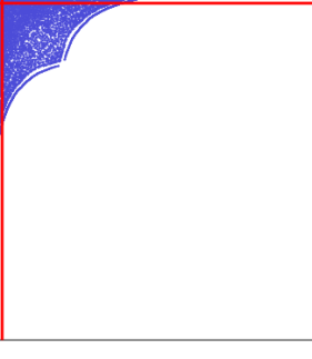
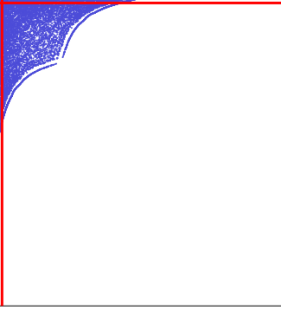
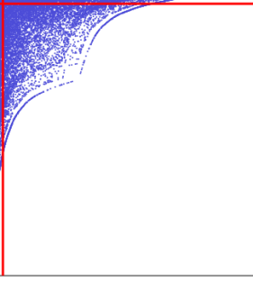
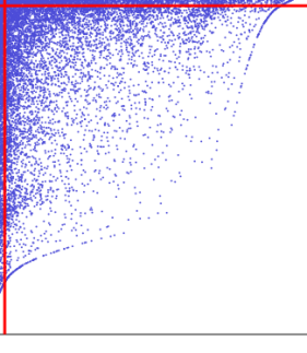
ML degree opt.
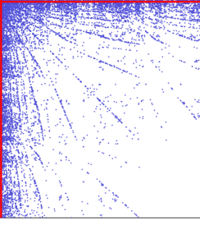
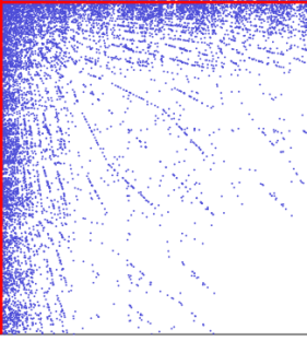
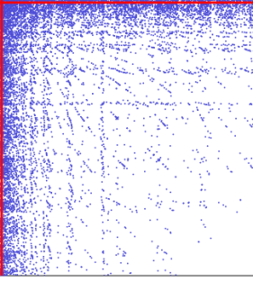
	$\bm{c}=[1,0]^{T}$	$\bm{c}=\bm{1}$	$\bm{c}=\bm{1}$	$\bm{c}=\bm{1}$
NSM aggr. eq.
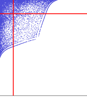
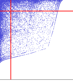
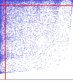
ML degree eq.

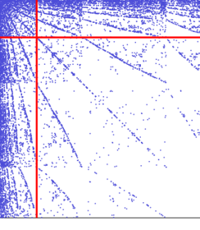
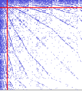
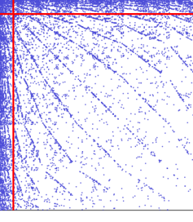
Figure 1: Reordered adjacency matrices of the informative layer of the two-layer Internet multiplex network for the parameters $\alpha=10,p=22$, and $q=2$ for various levels of noise in the second uninformative layer as well as optimized and equal layer weights.

	$0\%$ noise	$10\%$ noise	$25\%$ noise	$50\%$ noise
	$\bm{c}=[1,0]^{T}$	$\bm{c}=[0.9966,0.8870]^{T}$	$\bm{c}=[0.9918,0.9215]^{T}$	$\bm{c}=[0.9843,0.9459]^{T}$
MP NSM
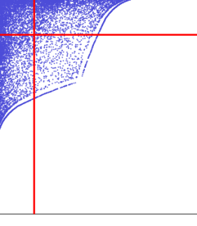
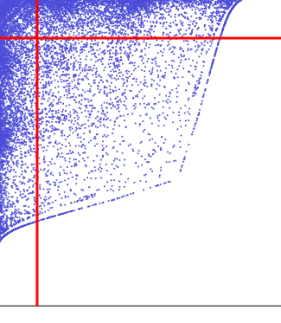
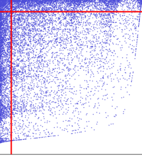
ML degree opt.

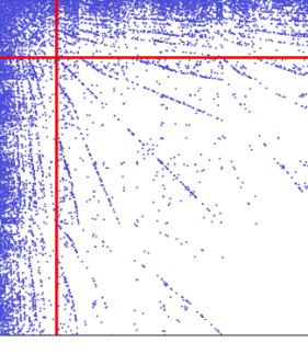
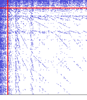
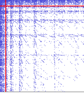
Figure 2: Reordered adjacency matrices of the informative layer of the two-layer Internet multiplex network for the parameters $\alpha=10$ and $p=q=22$ for various levels of noise in the second uninformative layer and optimized layer weights. The results for equal layer weights coincide with those displayed in Figure 1.

	$0\%$ noise	$10\%$ noise	$25\%$ noise	$50\%$ noise
	$\bm{c}=[1,0]^{T}$	$\bm{c}=[0.9999,0.0008]^{T}$	$\bm{c}=[0.9999,0.0022]^{T}$	$\bm{c}=[0.9999,0.0038]^{T}$
MP NSM
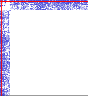
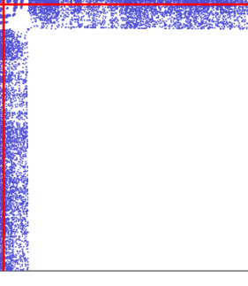
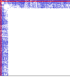
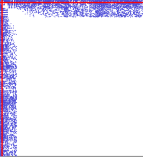
ML degree opt.
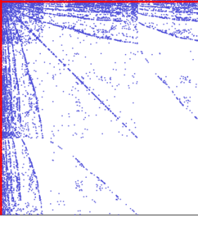
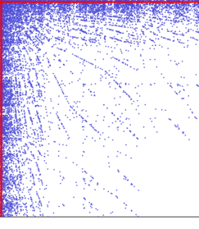
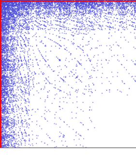
	$\bm{c}=[1,0]^{T}$	$\bm{c}=\bm{1}$	$\bm{c}=\bm{1}$	$\bm{c}=\bm{1}$
NSM aggr. eq.

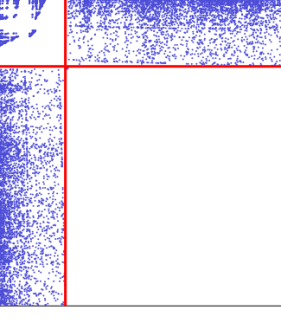
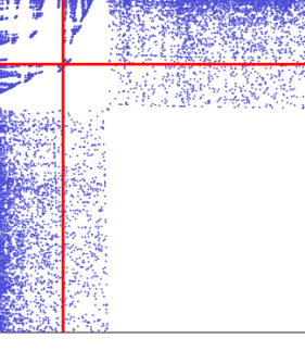
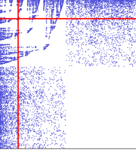
Figure 3: Reordered adjacency matrices of the informative layer of the two-layer Internet multiplex network for the parameters $\alpha=10$ and $p=q=2$ for various levels of noise in the second uninformative layer as well as optimized and equal layer weights. The results of ML degree eq. coincide with those displayed in Figure 1.

In all our experiments, we compare the performance of the optimized layer weight vector $\bm{c}$ returned by Algorithm 1 for the specified choice of $q$ with equal layer weights corresponding to the limit case $q\rightarrow\infty$.

In Tables 1 and 2, we compare the maximal multiplex QUBO values and the corresponding optimal core sizes $s^{\ast}$ for the four artificial multiplex networks and for five different core-periphery detection methods, cf. Section 5. In addition to our method (MP NSM) and the multilayer degree method (ML degree) [1], we report results of the core-periphery detection methods h-index [35], EigA [8], EigQ [27], and single-layer NSM [46] applied to the aggregated networks using the indicated layer weight vector $\bm{c}$. We observe throughout all experiments that MP NSM with $p=q=2$ obtains the best and MP NSM with $p=22$ and $q=2$ the second best multiplex QUBO scores indicating reordered adjacency matrices close to the ideal L-shape. Maximal multiplex QUBO scores of ML degree typically range slightly below those of MP NSM obtained with the same layer weight vector $\bm{c}$.

$10\%$ noise

$25\%$ noise

$50\%$ noise

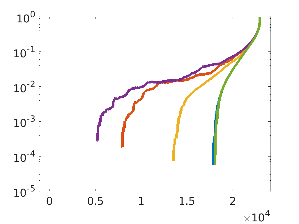
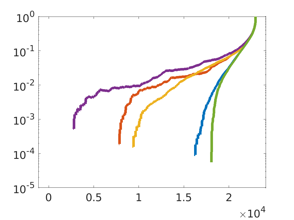
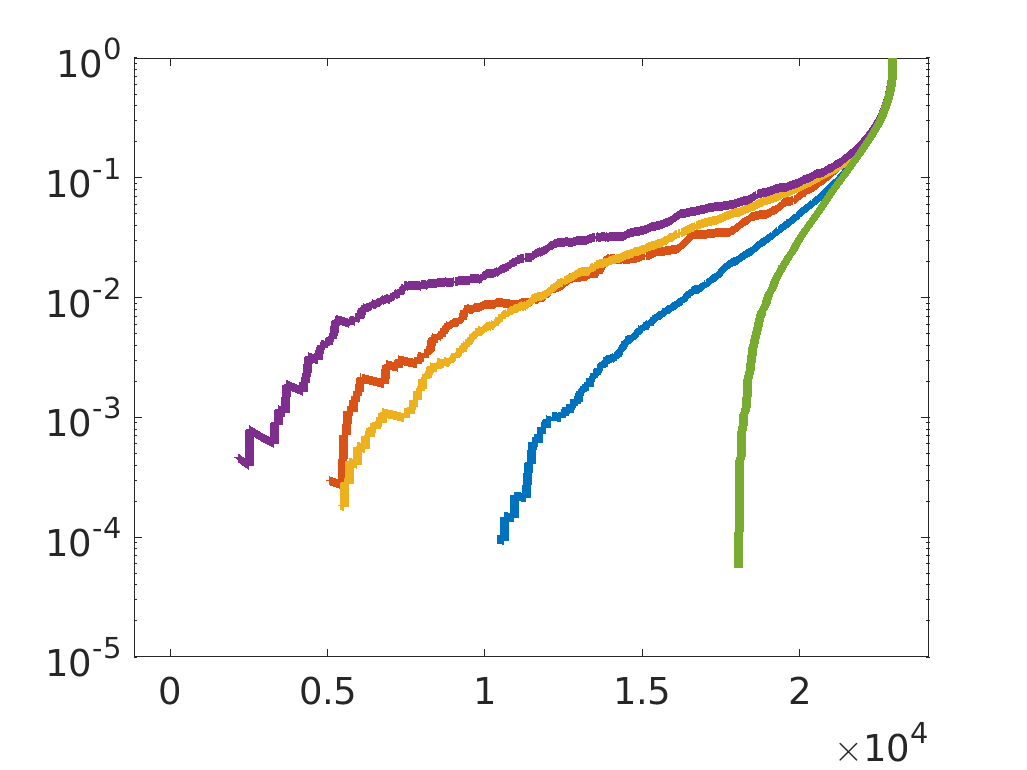
(a) $p=22,q=2$

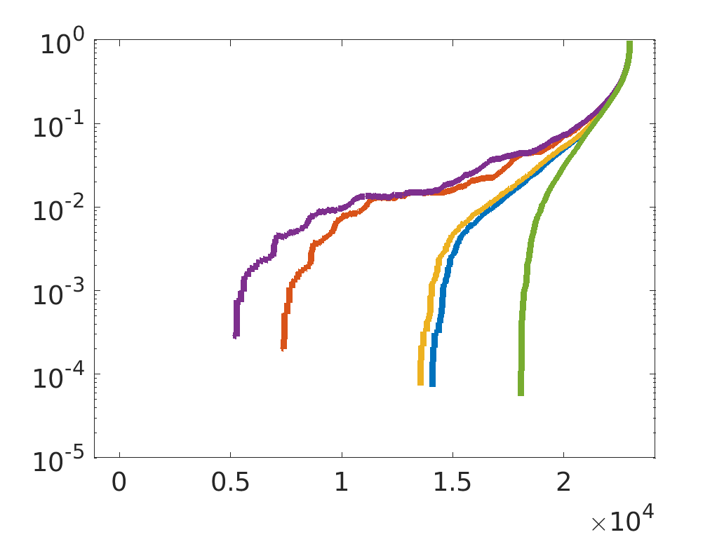
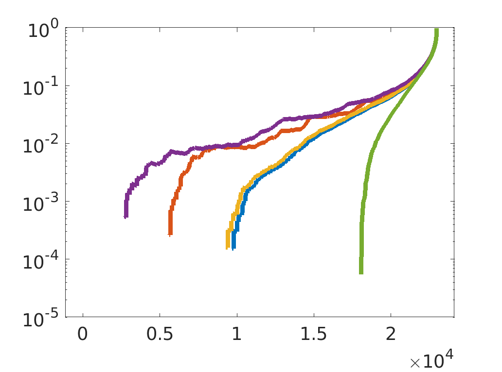
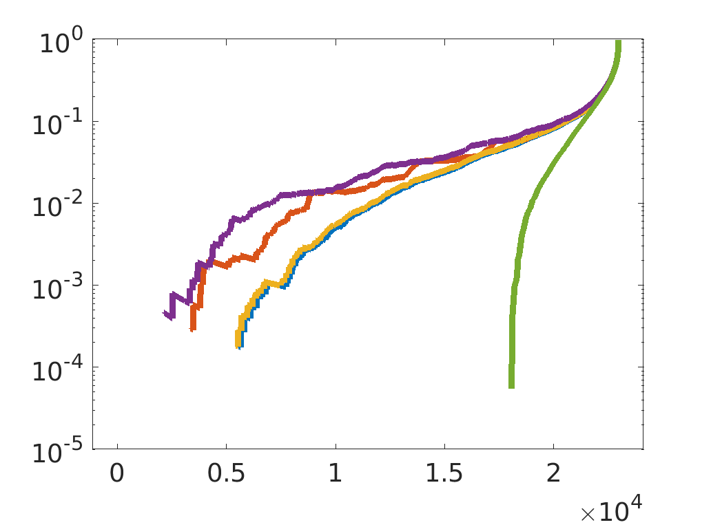
(b) $p=q=22$

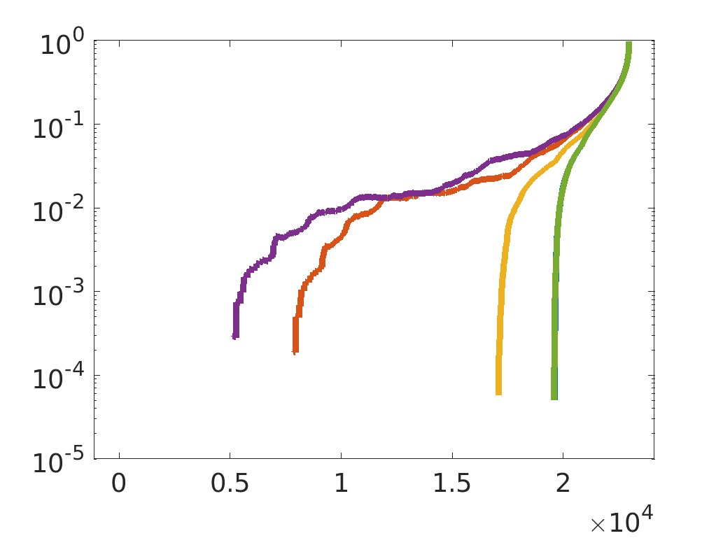
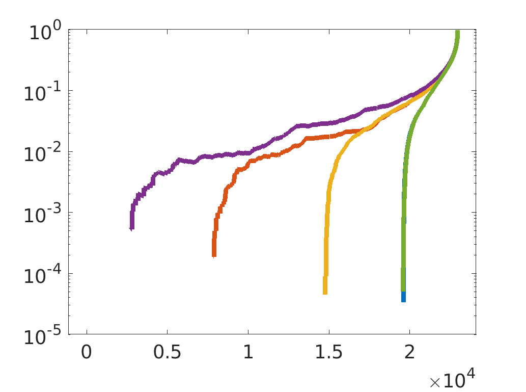
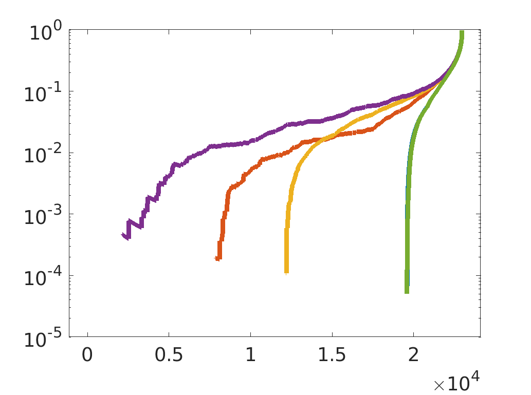
(c) $p=q=2$

Figure 4: Single-layer core-periphery profiles on the informative layer of the two-layer Internet multiplex network for different choices of the parameters $p$ and $q$. In panel (c), the green and blue curves of MP NSM and NSM single-layer lie almost on top of each other.

As is to be expected, an increasing noise level negatively affects the correct recovery of the core-periphery structure of the informative layer. Furthermore, we observe significantly better results with the layer weight vectors $\bm{c}$ optimized by MP NSM compared to equal weights throughout all methods since the optimized weights assign less weight to the uninformative noise layer. The parameter setting $p=q=2$ that only guarantees convergence to local optima proves to be particularly robust against noise. One consequence of these observations is that our novel optimized layer weights significantly improve the multilayer degree method [1].

As described in Section 5, alternative means of assessing the quality of a given core-periphery partition are by visual inspection of the reordered adjacency matrices as well as by random walk core-periphery profiles. Since by construction, we have one informative and one noisy layer in the experiments of this subsection, we apply both techniques only to the informative layer to assess the negative impact of the additional noise layer.

Figures 1, 2, and 3 show sparsity plots of the reordered Internet network with one additional noise layer for different choices of the parameters $p$ and $q$ in the multiplex nonlinear spectral method. ML degree opt. refers to Eq. 3 with $\bm{c}$ optimized by MP NSM while NSM aggr. eq. and ML degree eq. refer to the single-layer versions of the respective method applied to the aggregated network using equal layer weights. The red lines indicate the ideal core size $s^{\ast}$. The figures show that throughout all considered parameter settings, the reorderings of MP NSM are visually closer to the ideal L-shape than those of ML degree. Additionally, the multiplex QUBO results from Tables 1 and 2 are confirmed in the sense that the optimized layer weights provide visually superior results in comparison to equal weights.

The parameter choice $p=22$ in Figures 1 and 2 satisfies the assumptions of Theorem 3.1 and hence guarantees display of the globally optimal solution. The relatively large parameter $q=22$ leads to layer weight vectors $\bm{c}$ that are relatively close to equal weights, e.g., the MP NSM results in Figure 2 are similar to the NSM aggr. eq. results in Figure 1. We mention again that we obtain $\bm{c}=\bm{1}$ in the limit case $q\rightarrow\infty$.

Figure 3 uses the parameters $p=q=2$, which do not guarantee convergence to a global optimum. Instead, we display the locally optimal solution as ensured by Theorem 3.2 obtained with the starting vectors $\bm{x}_{0}=\bm{1}\in\mathbb{R}^{n}$ and $\bm{c}_{0}=\bm{1}\in\mathbb{R}^{L}$. In practice, different positive starting vectors $\bm{x}_{0}$ and $\bm{c}_{0}$ lead to slightly different solution vectors $\bm{x}$ and $\bm{c}$, but we found them to give rise to very similar reordered adjacency matrices. The case $p=q=2$ yields qualitatively different results in the sense that more L-shaped reorderings are obtained. Remarkably, this parameter setting is extremely robust against noise as the optimized layer weight vector $\bm{c}$ remains close to the first unit vector for all considered noise levels. In terms of the optimal core size $s^{\ast}$, which the single-layer NSM and degree method agree on ranging between $1\,100$ and $1\,200$, we see that the additional noise layer obfuscates this optimal core size in all settings but in those where the optimized layer weights obtained by $q=2$ are used in either method.

Finally, the visual observations are quantitatively confirmed by the random walk core-periphery profiles defined in Section 5 applied to the informative layer. A good core-periphery partition is characterized by a sharp increase in the random walk profile for a large index. Figure 4 shows that for this measure, the layer weights optimized by the multiplex nonlinear spectral method outperform equal weights for MP NSM and ML degree in all parameter settings. The random walk core-periphery profiles of MP NSM with $p=22$ are degrading with increasing noise level while they are visually indistinguishable from the single-layer result for $p=2$. In particular, the single-layer random walk core-periphery profile obtained with $p=2$ is superior to that of $p=22$ although unique global optimality is only guaranteed for $p=22$.

The runtime of Algorithm 1 for the computationally most expensive experiment in this section, i.e., the email-EU All multiplex network with $25\%$ noise is $2.25$ seconds for $28$ iterations with the parameters $p=22,q=2$, as well as $4.34$ seconds for $59$ iterations with the parameters $p=2,q=2$.

6.2 Real-world multiplex networks

The second set of experiments is performed on real-world multiplex networks. This situation is challenging since it is generally not known a-priori whether all layers contain a core-periphery structure and, in case they do, to what extent the sets of core nodes overlap. We inspected random walk core-periphery profiles on individual layers of several multiplex networks for different parameters $q$ in the multiplex nonlinear spectral method leading to layer weight vectors $\bm{c}$ ranging between being close to a unit vector and being close to the vector of all ones. We found the best choice of $q$ to be dataset-dependent, i.e., small values of $q$ perform well if noise is present in some layers and the corresponding layer weight is close to $0$ while large values of $q$ perform well if the informativity is equally distributed across the layers. It was often observed that the improvement of the core-periphery structure in one layer entails its deterioration in other layers.

In this section, we consider the following seven real-world multiplex networks with symmetrized and binarized layers.

Arabidopsis multiplex GPI network (Arabid.) [44, 18], genetic interaction network with $L=7$ different types of interactions between the $n=6\,980$ genes of “Arabidopsis Thaliana”.

Arxiv netscience multiplex (Arxiv) [17], scientific collaboration network with $L=13$ different arXiv categories and co-authorship relations between $n=14\,489$ network scientists.

Drosophila multiplex GPI network (Drosoph.) [44, 18], genetic interaction network with $L=7$ different types of interactions between the $n=8\,215$ genes of “Drosophila Melanogaster”.

EU-Air transportation multiplex (EU air.) [12], European airline transportation network with $L=37$ different airlines and their flight connections between $n=417$ European airports.

Homo multiplex GPI network (Homo) [44, 19], genetic interaction network with $L=7$ different types of interactions between the $n=18\,222$ genes of “Homo Sapiens”.

Twitter Rana Plaza year $2013$ (TRP ’13) [5], Twitter network with $L=3$ different types of interactions between $n=9\,925$ users.

Twitter Rana Plaza year $2014$ (TRP ’14) [5], Twitter network with $L=3$ different types of interactions between $n=14\,866$ users.

Table 3 summarizes maximal multiplex QUBO values and optimal core sizes for these networks. We compare the same core-periphery detection methods considered in Tables 1 and 2 on aggregated versions of the seven multiplex networks using the indicated layer weight vectors $\bm{c}$. Furthermore, we compare different parameter settings of the multiplex nonlinear spectral method. In the cases of optimized weights, we choose the parameter $q=2$ while the equal weights case corresponds to the limit case $q\rightarrow\infty$.

Table 3 shows that the maximal multiplex QUBO value is obtained by the multiplex nonlinear spectral method in the parameter setting $p=q=2$ for all but one data set. However, the second largest value is distributed more homogeneously across different methods and parameter settings. As described earlier in this subsection, it depends on the distribution of core-periphery structure across the layers whether weights optimized with $q=2$ or equal weights lead to better multiplex core-periphery partitions.

Network		Arabid.	Arxiv	Drosoph.	EU Air.	Homo	TRP ’13	TRP ’14
$p=22$, opt. weights
MP NSM	score	$0.6431$	$0.4105$	$0.5210$	$0.5768$	$0.6974$	0.8154	0.7499
	size	(746)	(1 517)	(1 220)	(67)	(1 522)	(524)	(1 078)
ML degree	score	$0.6207$	$0.3930$	$0.5105$	$0.5626$	$0.6878$	$0.7921$	$0.7260$
	size	(581)	(1 408)	(1 239)	(68)	(1 709)	(408)	(1 046)
h-index	score	$0.1526$	$0.1792$	$0.0954$	$0.4421$	$0.4101$	$0.2334$	$0.2133$
	size	(939)	(2 063)	(1 524)	(83)	(4 156)	(1 538)	(2 206)
EigA	score	$0.3299$	$0.2232$	$0.4380$	$0.4288$	$0.6368$	$0.3101$	$0.3569$
	size	(1 380)	(1 544)	(1 236)	(111)	(1 584)	(3 782)	(2 452)
EigQ	score	$0.2458$	$0.2294$	$0.3976$	$0.4645$	$0.4340$	$0.7670$	$0.4308$
	size	(836)	(1 459)	(1 895)	(99)	(3 367)	(778)	(3 009)
$p=22$, eq. weights
NSM	score	$0.6277$	$0.3421$	$0.5070$	$0.6384$	$0.7239$	$0.7962$	$0.7304$
	size	(597)	(2 225)	(2 075)	(40)	(1 305)	(539)	(1 120)
ML degree	score	$0.6090$	$0.3212$	$0.4755$	0.6397	$0.7198$	$0.7631$	$0.7000$
	size	(623)	(1 556)	(1 143)	(46)	(1 395)	(638)	(1 148)
h-index	score	$0.4480$	$0.1404$	$0.0404$	$0.5045$	$0.4453$	$0.2384$	$0.2528$
	size	(374)	(2 100)	(336)	(83)	(4 141)	(1 538)	(2 206)
EigA	score	$0.2487$	$0.1445$	$0.3671$	$0.6234$	$0.6729$	$0.2819$	$0.3663$
	size	(1 870)	(985)	(2 703)	(46)	(1 552)	(1 729)	(2 712)
EigQ	score	$0.4220$	$0.3077$	0.6170	$0.5103$	$0.5332$	$0.7919$	$0.4773$
	size	(214)	(2 384)	(864)	(43)	(1 665)	(777)	(2 811)
$p=2$, opt. weights
MP NSM	score	0.8563	0.4834	0.5462	0.6463	0.7629	0.8292	0.7651
	size	(306)	(1 719)	(1 279)	(63)	(1 309)	(553)	(1 229)
ML degree	score	0.8249	0.4382	$0.5211$	$0.5987$	0.7369	$0.7946$	$0.7277$
	size	(332)	(1 698)	(1 187)	(43)	(1 366)	(406)	(1 039)
h-index	score	$0.3197$	$0.1917$	$0.1223$	$0.3820$	$0.6941$	$0.2332$	$0.2124$
	size	(2 729)	(1 414)	(1 899)	(78)	(1 550)	(1 538)	(2 206)
EigA	score	$0.5064$	$0.2580$	$0.4358$	$0.5110$	$0.6788$	$0.3066$	$0.3599$
	size	(89)	(1 581)	(1 222)	(42)	(1 599)	(3 310)	(2 460)
EigQ	score	$0.4539$	$0.2305$	$0.3797$	$0.4430$	$0.4160$	$0.7652$	$0.4280$
	size	(210)	(1 444)	(2 057)	(99)	(3 169)	(778)	(3 105)
$p=2$, eq. weights
NSM	score	$0.6291$	$0.3780$	0.5462	$0.6360$	$0.7246$	$0.8141$	$0.7470$
	size	(570)	(1 927)	(1 427)	(45)	(1 411)	(541)	(1 264)

Table 3: Multiplex QUBO score and optimal core size $s^{\ast}$ for seven real-world multiplex networks. Optimized weights correspond to the parameter choice $q=2$ while equal weights refer to the limit case $q\rightarrow\infty$.

	Layer 1	Layer 2	Layer 3
	$\bm{c}=[0.3439,0.0241,0.9387]^{T}$
MP NSM
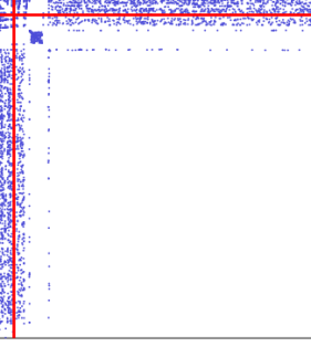
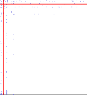
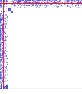
ML degree opt.
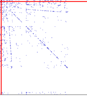
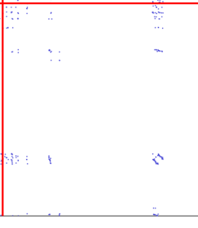
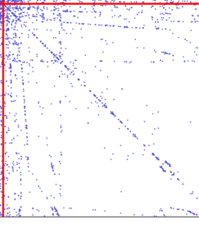
	$\bm{c}=\bm{1}$
NSM aggr. eq.
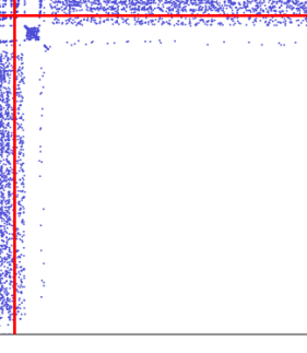
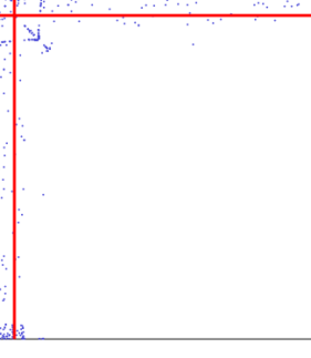
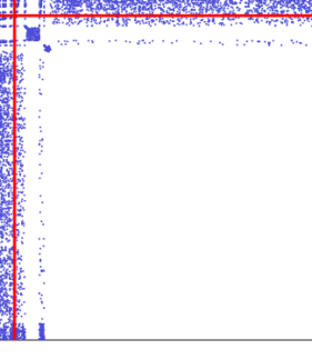
ML degree eq.

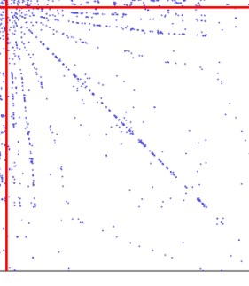
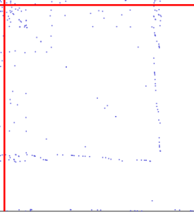
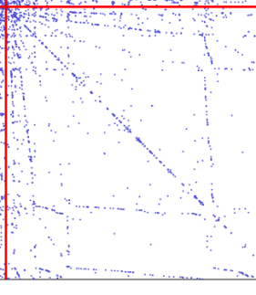
Figure 5: Layer-wise reordered adjacency matrices of the Twitter Rana Plaza $2014$ multiplex network with parameters $\alpha=10$ and $p=2$. Optimized layer weights correspond to $q=2$.

Throughout all but one numerical example, the multiplex QUBO values of the multilayer degree method range slightly below those of MP NSM. Section 6.1 showed that albeit these small differences in multiplex QUBO values, the visual and random walk-based evaluation of multiplex core-periphery structures indicates superiority of the multiplex nonlinear spectral method. The same observation holds true in the case of real-world multiplex networks. Figure 5 exemplarily shows that the visual reordering for the Twitter Rana Plaza $2014$ network obtained by MP NSM is much closer to an ideal L-shape than that obtained by ML degree.

The runtime of Algorithm 1 for the computationally most expensive experiment in this section, i.e., the homo multiplex network is $0.69$ seconds for $26$ iterations with the parameters $p=22,q=2$, as well as $3.18$ seconds for $124$ iterations with the parameters $p=2,q=2$.

7 Conclusion

In this work, we proposed a nonlinear spectral method for multiplex core-periphery detection that simultaneously optimizes a node and a layer coreness vector. We provided convergence guarantees to global and local optima, discussed the detection of optimal core sizes, and illustrated that our method outperforms the state of the art on various synthetic and real-world multiplex networks.

Future work could consider more general multilayer networks with directed or weighted edges as well as inter-layer edges, i.e., edges across layers.

Appendix A Proof of Theorem 3.1

We require the following two Lemmas before we turn to the proof of Theorem 3.1.

Lemma A.1.

The objective function $f_{\alpha}(\bm{x},\bm{c})$ defined in Eq. 4 satisfies the elementwise inequalities

(13) $$\begin{array}[]{cc}|\nabla_{\bm{x}}\nabla_{\bm{x}}f_{\alpha}(\bm{x},\bm{c})\bm{x}|\leq\bm{\Theta}_{11}|\nabla_{\bm{x}}f_{\alpha}(\bm{x},\bm{c})|&|\nabla_{\bm{c}}\nabla_{\bm{x}}f_{\alpha}(\bm{x},\bm{c})\bm{c}|\leq\bm{\Theta}_{12}|\nabla_{\bm{x}}f_{\alpha}(\bm{x},\bm{c})|\\ |\nabla_{\bm{x}}\nabla_{\bm{c}}f_{\alpha}(\bm{x},\bm{c})\bm{x}|\leq\bm{\Theta}_{21}|\nabla_{\bm{c}}f_{\alpha}(\bm{x},\bm{c})|&|\nabla_{\bm{c}}\nabla_{\bm{c}}f_{\alpha}(\bm{x},\bm{c})\bm{c}|\leq\bm{\Theta}_{22}|\nabla_{\bm{c}}f_{\alpha}(\bm{x},\bm{c})|\end{array}$$

with the coefficient matrix

$$\bm{\Theta}=\begin{bmatrix}\bm{\Theta}_{11}&\bm{\Theta}_{12}\\ \bm{\Theta}_{21}&\bm{\Theta}_{22}\end{bmatrix}=\begin{bmatrix}|\alpha-1|&1\\ 2&0\end{bmatrix}.$$

Proof A.2.

Throughout the proof, sums over $i$ and $j$ include indices $i,j=1,\dots,n$ while sums over $k$ include indices $k=1,\dots,L$. The entries of the gradients of Eq. 4 read

$$\left[\nabla_{\bm{x}}f_{\alpha}(\bm{x},\bm{c})\right]_{m}=2\sum_{j}\bm{x}_{m}^{\alpha-1}(\bm{x}_{m}^{\alpha}+\bm{x}_{j}^{\alpha})^{1/\alpha-1}\sum_{k}\bm{c}_{k}\bm{A}_{mj}^{(k)},\quad\left[\nabla_{\bm{c}}f_{\alpha}(\bm{x},\bm{c})\right]_{l}=\sum_{i,j}\bm{A}_{ij}^{(l)}(\bm{x}_{i}^{\alpha}+\bm{x}_{j}^{\alpha})^{1/\alpha}.$$

Furthermore, the entries of the Hessian of Eq. 4 read

$$[\nabla_{\bm{x}}\nabla_{\bm{x}}f_{\alpha}(\bm{x},\bm{c})]_{mi} =2(1-\alpha)\bm{x}_{m}^{\alpha-1}\bm{x}_{i}^{\alpha-1}(\bm{x}_{m}^{\alpha}+\bm{x}_{i}^{\alpha})^{1/\alpha-2}\sum_{k}\bm{c}_{k}\bm{A}_{mi}^{(k)},\quad\text{ for }m\neq i,$$

$$[\nabla_{\bm{x}}\nabla_{\bm{x}}f_{\alpha}(\bm{x},\bm{c})]_{mm} =2(\alpha-1)\bm{x}_{m}^{\alpha-2}\sum_{\begin{subarray}{c}j\\ j\neq m\end{subarray}}\bm{x}_{j}^{\alpha}(\bm{x}_{m}^{\alpha}+\bm{x}_{j}^{\alpha})^{1/\alpha-2}\sum_{k}\bm{c}_{k}\bm{A}_{mj}^{(k)},$$

$$[\nabla_{\bm{x}}\nabla_{\bm{c}}f_{\alpha}(\bm{x},\bm{c})]_{ml} =[\nabla_{\bm{c}}\nabla_{\bm{x}}f_{\alpha}(\bm{x},\bm{c})]_{lm}=2\sum_{j}\bm{A}_{mj}^{(l)}\bm{x}_{m}^{\alpha-1}(\bm{x}_{m}^{\alpha}+\bm{x}_{j}^{\alpha})^{1/\alpha-1},$$

$$\nabla_{\bm{c}}\nabla_{\bm{c}}f_{\alpha}(\bm{x},\bm{c}) =\bm{0}.$$

Note that since $\alpha>1$ by assumption, all gradient and Hessian entries except for $[\nabla_{\bm{x}}\nabla_{\bm{x}}f_{\alpha}(\bm{x},\bm{c})]_{mi}$ for $m\neq i$ are non-negative.

Since $\nabla_{\bm{c}}\nabla_{\bm{c}}f_{\alpha}(\bm{x},\bm{c})=\bm{0}$, we have $\bm{\Theta}_{22}=0$ and by

$$[\nabla_{\bm{c}}\nabla_{\bm{x}}f_{\alpha}(\bm{x},\bm{c})\bm{c}]_{m}=2\sum_{j}\bm{x}_{m}^{\alpha-1}(\bm{x}_{m}^{\alpha}+\bm{x}_{j}^{\alpha})^{1/\alpha-1}\sum_{k}\bm{c}_{k}\bm{A}_{mj}^{(k)}=\left[\nabla_{\bm{x}}f_{\alpha}(\bm{x},\bm{c})\right]_{m},$$

we immediately see $\bm{\Theta}_{12}=1$.

To obtain $\bm{\Theta}_{21}=2$, consider

$$[\nabla_{\bm{x}}\nabla_{\bm{c}}f_{\alpha}(\bm{x},\bm{c})\bm{x}]_{l} =2\sum_{i,j}\bm{A}_{ij}^{(l)}\bm{x}_{i}^{\alpha}(\bm{x}_{i}^{\alpha}+\bm{x}_{j}^{\alpha})^{1/\alpha-1}$$

$$\leq 2\sum_{i,j}\bm{A}_{ij}^{(l)}(\bm{x}_{i}^{\alpha}+\underbrace{\bm{x}_{j}^{\alpha}}_{\geq 0})(\bm{x}_{i}^{\alpha}+\bm{x}_{j}^{\alpha})^{1/\alpha-1}=2[\nabla_{\bm{c}}f_{\alpha}(\bm{x},\bm{c})]_{l}$$

for all $l=1,\dots,L$.

Finally, for $\bm{\Theta}_{11}$, we consider the cases $i\neq m$ and $i=m$ separately. For $i\neq m$, we have

$$\frac{[\nabla_{\bm{x}}\nabla_{\bm{x}}f_{\alpha}(\bm{x},\bm{c})]_{mi}\bm{x}_{i}}{[\nabla_{\bm{x}}f_{\alpha}(\bm{x},\bm{c})]_{m}} =\frac{2(1-\alpha)\bm{x}_{m}^{\alpha-1}\bm{x}_{i}^{\alpha}(\bm{x}_{m}^{\alpha}+\bm{x}_{i}^{\alpha})^{1/\alpha-2}\sum_{k}\bm{c}_{k}\bm{A}_{mi}^{(k)}}{2\sum_{j}\bm{x}_{m}^{\alpha-1}(\bm{x}_{m}^{\alpha}+\bm{x}_{j}^{\alpha})^{1/\alpha-1}\sum_{k}\bm{c}_{k}\bm{A}_{mj}^{(k)}}$$

$$=(1-\alpha)\frac{\bm{x}_{i}^{\alpha}}{\bm{x}_{m}^{\alpha}+\bm{x}_{i}^{\alpha}}\frac{(\bm{x}_{m}^{\alpha}+\bm{x}_{i}^{\alpha})^{1/\alpha-1}\sum_{k}\bm{c}_{k}\bm{A}_{mi}^{(k)}}{\sum_{j}(\bm{x}_{m}^{\alpha}+\bm{x}_{j}^{\alpha})^{1/\alpha-1}\sum_{k}\bm{c}_{k}\bm{A}_{mj}^{(k)}}$$

$$\geq(1-\alpha)\frac{(\bm{x}_{m}^{\alpha}+\bm{x}_{i}^{\alpha})^{1/\alpha-1}\sum_{k}\bm{c}_{k}\bm{A}_{mi}^{(k)}}{\sum_{j}(\bm{x}_{m}^{\alpha}+\bm{x}_{j}^{\alpha})^{1/\alpha-1}\sum_{k}\bm{c}_{k}\bm{A}_{mj}^{(k)}},$$

since, by assumption, we have $\alpha>1\Leftrightarrow 1-\alpha<0$.

Summing over $i=\{1,\dots,n\}\setminus\{m\}$ yields

$$\frac{\sum_{\begin{subarray}{c}i\\ i\neq m\end{subarray}}[\nabla_{\bm{x}}\nabla_{\bm{x}}f_{\alpha}(\bm{x},\bm{c})]_{mi}\bm{x}_{i}}{[\nabla_{\bm{x}}f_{\alpha}(\bm{x},\bm{c})]_{m}} =(1-\alpha)\frac{\sum_{\begin{subarray}{c}i\\ i\neq m\end{subarray}}(\bm{x}_{m}^{\alpha}+\bm{x}_{i}^{\alpha})^{1/\alpha-1}\sum_{k}\bm{c}_{k}\bm{A}_{mi}^{(k)}}{\sum_{j}(\bm{x}_{m}^{\alpha}+\bm{x}_{j}^{\alpha})^{1/\alpha-1}\sum_{k}\bm{c}_{k}\bm{A}_{mj}^{(k)}}$$

$$\geq(1-\alpha).$$

Moreover, since all summands of $\sum_{\begin{subarray}{c}i\\ i\neq m\end{subarray}}(\bm{x}_{m}^{\alpha}+\bm{x}_{i}^{\alpha})^{1/\alpha-1}\sum_{k}\bm{c}_{k}\bm{A}_{mi}^{(k)}$ and $\sum_{j}(\bm{x}_{m}^{\alpha}+\bm{x}_{j}^{\alpha})^{1/\alpha-1}\sum_{k}\bm{c}_{k}\bm{A}_{mj}^{(k)}$ are non-negative, we have

$$\frac{\sum_{\begin{subarray}{c}i\\ i\neq m\end{subarray}}[\nabla_{\bm{x}}\nabla_{\bm{x}}f_{\alpha}(\bm{x},\bm{c})]_{mi}\bm{x}_{i}}{[\nabla_{\bm{x}}f_{\alpha}(\bm{x},\bm{c})]_{m}}\leq 0.$$

For $i=m$, we have

$$\frac{[\nabla_{\bm{x}}\nabla_{\bm{x}}f_{\alpha}(\bm{x},\bm{c})]_{mm}\bm{x}_{m}}{[\nabla_{\bm{x}}f_{\alpha}(\bm{x},\bm{c})]_{m}} =\frac{2(\alpha-1)\bm{x}_{m}^{\alpha-1}\sum_{\begin{subarray}{c}j\\ j\neq m\end{subarray}}\bm{x}_{j}^{\alpha}(\bm{x}_{m}^{\alpha}+\bm{x}_{j}^{\alpha})^{1/\alpha-2}\sum_{k}\bm{c}_{k}\bm{A}_{mj}^{(k)}}{2\sum_{j}\bm{x}_{m}^{\alpha-1}(\bm{x}_{m}^{\alpha}+\bm{x}_{j}^{\alpha})^{1/\alpha-1}\sum_{k}\bm{c}_{k}\bm{A}_{mj}^{(k)}}$$

$$=(\alpha-1)\frac{\sum_{\begin{subarray}{c}j\\ j\neq m\end{subarray}}\frac{\bm{x}_{j}^{\alpha}}{\bm{x}_{m}^{\alpha}+\bm{x}_{j}^{\alpha}}(\bm{x}_{m}^{\alpha}+\bm{x}_{j}^{\alpha})^{1/\alpha-1}\sum_{k}\bm{c}_{k}\bm{A}_{mj}^{(k)}}{\sum_{j}(\bm{x}_{m}^{\alpha}+\bm{x}_{j}^{\alpha})^{1/\alpha-1}\sum_{k}\bm{c}_{k}\bm{A}_{mj}^{(k)}}$$

$$\leq(\alpha-1)\frac{\sum_{\begin{subarray}{c}j\\ j\neq m\end{subarray}}(\bm{x}_{m}^{\alpha}+\bm{x}_{j}^{\alpha})^{1/\alpha-1}\sum_{k}\bm{c}_{k}\bm{A}_{mj}^{(k)}}{\sum_{j}(\bm{x}_{m}^{\alpha}+\bm{x}_{j}^{\alpha})^{1/\alpha-1}\sum_{k}\bm{c}_{k}\bm{A}_{mj}^{(k)}}$$

$$\leq(\alpha-1).$$

At the same time, we have $\frac{[\nabla_{\bm{x}}\nabla_{\bm{x}}f_{\alpha}(\bm{x},\bm{c})]_{mm}\bm{x}_{m}}{[\nabla_{\bm{x}}f_{\alpha}(\bm{x},\bm{c})]_{m}}\geq 0$ since all elements are non-negative.

Finally, we obtain

$$(1-\alpha)\leq\sum_{\begin{subarray}{c}i\\ i\neq m\end{subarray}}[\nabla_{\bm{x}}\nabla_{\bm{x}}f_{\alpha}(\bm{x},\bm{c})]_{mi}\bm{x}_{i}+[\nabla_{\bm{x}}\nabla_{\bm{x}}f_{\alpha}(\bm{x},\bm{c})]_{mm}\bm{x}_{m}\leq(\alpha-1)$$

$$\Leftrightarrow ~{}\frac{\left|\sum_{\begin{subarray}{c}i\\ i\neq m\end{subarray}}[\nabla_{\bm{x}}\nabla_{\bm{x}}f_{\alpha}(\bm{x},\bm{c})]_{mi}\bm{x}_{i}+[\nabla_{\bm{x}}\nabla_{\bm{x}}f_{\alpha}(\bm{x},\bm{c})]_{mm}\bm{x}_{m}\right|}{|[\nabla_{\bm{x}}f_{\alpha}(\bm{x},\bm{c})]_{m}|}\leq|\alpha-1|\color[rgb]{0,0,0}=\bm{\Theta}_{11}.$$

Again using the notation $J_{p}(\bm{x}):=\nabla\|\bm{x}\|_{p}=\|\bm{x}\|_{p}^{1-p}\bm{x}^{p-1}$, we define the fixed point map

(14) $$G^{\alpha}(\bm{x},\bm{c}):=\begin{bmatrix}\nabla_{\bm{x}}g_{\alpha}(\bm{x},\bm{c})\\ \nabla_{\bm{c}}g_{\alpha}(\bm{x},\bm{c})\end{bmatrix}=\begin{bmatrix}J_{p^{\ast}}(\nabla_{\bm{x}}f_{\alpha}(\bm{x},\bm{c}))\\ J_{q^{\ast}}(\nabla_{\bm{c}}f_{\alpha}(\bm{x},\bm{c}))\end{bmatrix}:=\begin{bmatrix}G^{\alpha}_{1}(\bm{x},\bm{c})\\ G^{\alpha}_{2}(\bm{x},\bm{c})\end{bmatrix},$$

corresponding to the iteration Eq. 7. We denote by $D_{\bm{x}}G^{\alpha}_{i}(\bm{x},\bm{c})$ and $D_{\bm{c}}G^{\alpha}_{i}(\bm{x},\bm{c})$ for $i=1,2$ the Jacobians w.r.t. $\bm{x}$ and $\bm{c}$, respectively. Consequently, quantities such as $D_{\bm{x}}G^{\alpha}_{1}(\bm{x},\bm{c})\bm{x}$ denote matrix-vector products.

Lemma A.3.

For elementwise divisions, the map $G^{\alpha}$ defined in Eq. 14 satisfies the elementwise inequality

(15) $$\begin{bmatrix}\left\|\frac{D_{\bm{x}}G^{\alpha}_{1}(\bm{x},\bm{c})\bm{x}}{G^{\alpha}_{1}(\bm{x},\bm{c})}\right\|_{1}&\left\|\frac{D_{\bm{c}}G^{\alpha}_{1}(\bm{x},\bm{c})\bm{c}}{G^{\alpha}_{1}(\bm{x},\bm{c})}\right\|_{1}\\[6.99997pt] \left\|\frac{D_{\bm{x}}G^{\alpha}_{2}(\bm{x},\bm{c})\bm{x}}{G^{\alpha}_{2}(\bm{x},\bm{c})}\right\|_{1}&\left\|\frac{D_{\bm{c}}G^{\alpha}_{2}(\bm{x},\bm{c})\bm{c}}{G^{\alpha}_{2}(\bm{x},\bm{c})}\right\|_{1}\end{bmatrix}\leq\begin{bmatrix}\frac{2|\alpha-1|}{p-1}&\frac{1}{p-1}\\[6.99997pt] \frac{2}{q-1}&0\end{bmatrix}=:\bm{M}.$$

Proof A.4.

We define $F_{\bm{x}}^{\alpha}:=\nabla_{\bm{x}}f_{\alpha}(\bm{x},\bm{c}),F_{\bm{c}}^{\alpha}:=\nabla_{\bm{c}}f_{\alpha}(\bm{x},\bm{c}),\partial_{r}:=\frac{\partial}{\partial\bm{x}_{r}},\partial_{s}:=\frac{\partial}{\partial\bm{c}_{s}}$ and throughout this proof, sums over $i$ include indices $i=1,\dots n$ while sums over $k$ include indices $k=1,\dots,L$. By the product and the chain rule, we obtain

$$\frac{\partial_{r}\left[G_{1}^{\alpha}(\bm{x},\bm{c})\right]_{m}}{\left[G_{1}^{\alpha}(\bm{x},\bm{c})\right]_{m}} =\frac{\partial_{r}\left(\|F_{\bm{x}}^{\alpha}\|_{p^{\ast}}^{1-p^{\ast}}\left(\left[F_{\bm{x}}^{\alpha}\right]_{m}\right)^{p^{\ast}-1}\right)}{\|F_{\bm{x}}^{\alpha}\|_{p^{\ast}}^{1-p^{\ast}}\left(\left[F_{\bm{x}}^{\alpha}\right]_{m}\right)^{p^{\ast}-1}}=(p^{\ast}-1)\left\{\frac{\partial_{r}\left[F_{\bm{x}}^{\alpha}\right]_{m}}{\left[F_{\bm{x}}^{\alpha}\right]_{m}}-\frac{\partial_{r}\|F_{\bm{x}}^{\alpha}\|_{p^{\ast}}}{\|F_{\bm{x}}^{\alpha}\|_{p^{\ast}}}\right\}$$

$$=(p^{\ast}-1)\left\{\frac{\partial_{r}\left[F_{\bm{x}}^{\alpha}\right]_{m}}{\left[F_{\bm{x}}^{\alpha}\right]_{m}}-\frac{\sum_{i}\left[F_{\bm{x}}^{\alpha}\right]_{i}^{p^{\ast}-1}\partial_{r}\left[F_{\bm{x}}^{\alpha}\right]_{i}}{\|F_{\bm{x}}^{\alpha}\|_{p^{\ast}}^{p^{\ast}}}\right\}$$

(16) $$=(p^{\ast}-1)\left\{\frac{\partial_{r}\left[F_{\bm{x}}^{\alpha}\right]_{m}}{\left[F_{\bm{x}}^{\alpha}\right]_{m}}-\sum_{i}\left(\frac{\left[F_{\bm{x}}^{\alpha}\right]_{i}}{\|F_{\bm{x}}^{\alpha}\|_{p^{\ast}}}\right)^{p^{\ast}}\frac{\partial_{r}\left[F_{\bm{x}}^{\alpha}\right]_{i}}{\left[F_{\bm{x}}^{\alpha}\right]_{i}}\right\}$$

Analogous computations yield

(17) $$\frac{\partial_{s}\left[G_{1}^{\alpha}(\bm{x},\bm{c})\right]_{m}}{\left[G_{1}^{\alpha}(\bm{x},\bm{c})\right]_{m}} =(p^{\ast}-1)\left\{\frac{\partial_{s}\left[F_{\bm{x}}^{\alpha}\right]_{m}}{\left[F_{\bm{x}}^{\alpha}\right]_{m}}-\sum_{i}\left(\frac{\left[F_{\bm{x}}^{\alpha}\right]_{i}}{\|F_{\bm{x}}^{\alpha}\|_{p^{\ast}}}\right)^{p^{\ast}}\frac{\partial_{s}\left[F_{\bm{x}}^{\alpha}\right]_{i}}{\left[F_{\bm{x}}^{\alpha}\right]_{i}}\right\},$$

(18) $$\frac{\partial_{r}\left[G_{2}^{\alpha}(\bm{x},\bm{c})\right]_{l}}{\left[G_{2}^{\alpha}(\bm{x},\bm{c})\right]_{l}} =(q^{\ast}-1)\left\{\frac{\partial_{r}\left[F_{\bm{c}}^{\alpha}\right]_{l}}{\left[F_{\bm{c}}^{\alpha}\right]_{l}}-\sum_{k}\left(\frac{\left[F_{\bm{c}}^{\alpha}\right]_{k}}{\|F_{\bm{c}}^{\alpha}\|_{q^{\ast}}}\right)^{q^{\ast}}\frac{\partial_{r}\left[F_{\bm{c}}^{\alpha}\right]_{k}}{\left[F_{\bm{c}}^{\alpha}\right]_{k}}\right\},$$

(19) $$\frac{\partial_{s}\left[G_{2}^{\alpha}(\bm{x},\bm{c})\right]_{l}}{\left[G_{2}^{\alpha}(\bm{x},\bm{c})\right]_{l}} =(q^{\ast}-1)\left\{\frac{\partial_{s}\left[F_{\bm{c}}^{\alpha}\right]_{l}}{\left[F_{\bm{c}}^{\alpha}\right]_{l}}-\sum_{k}\left(\frac{\left[F_{\bm{c}}^{\alpha}\right]_{k}}{\|F_{\bm{c}}^{\alpha}\|_{q^{\ast}}}\right)^{q^{\ast}}\frac{\partial_{s}\left[F_{\bm{c}}^{\alpha}\right]_{k}}{\left[F_{\bm{c}}^{\alpha}\right]_{k}}\right\}.$$

Taking the absolute value of (16) leads to a quantity of the form $|\beta_{m}-\sum_{i}\gamma_{i}\beta_{i}|$, where $\gamma_{i}\geq 0$, $\sum_{i}\gamma_{i}=1$, and $\beta_{m}$ may be positive or negative. Defining $\widetilde{m}:=\text{argmax}_{m}|\beta_{m}|$, we have $|\beta_{m}-\sum_{i}\gamma_{i}\beta_{i}|\leq 2|\beta_{\widetilde{m}}|$.

The absolute value of (17) takes the same form, but here all $\beta_{m}$ are non-negative. Hence, we have $|\beta_{m}-\sum_{i}\gamma_{i}\beta_{i}|\leq|\beta_{\widetilde{m}}|$.

Absolute values of both (18) and (19) yield $|\beta_{l}-\sum_{k}\gamma_{k}\beta_{k}|$ with $\gamma_{k}\geq 0$, $\sum_{k}\gamma_{k}=1$, and $\beta_{l}$ non-negative such that we define $\widetilde{l}:=\text{argmax}_{l}|\beta_{l}|$ to find $|\beta_{l}-\sum_{k}\gamma_{k}\beta_{k}|\leq|\beta_{\widetilde{l}}|$ in both cases.

Then, multiplication with $\bm{x}_{m}\geq 0$ and $\bm{c}_{l}\geq 0$ as well as summation over $m$ and $l$, respectively, the bounds from Lemma A.1, as well as $p^{\ast}-1=\frac{1}{p-1}$ and $q^{\ast}-1=\frac{1}{q-1}$ yield the claim.

With these results at hand, we can prove the global convergence of Eq. 7, i.e., Algorithm 1 under the conditions stated in Theorem 3.1.

Proof A.5 (Proof of Theorem 3.1).

We show that $G^{\alpha}$ defined in Eq. 14 is contractive with respect to a suitable metric with Lipschitz constant $\rho(\bm{M})$. We start by recalling the Thompson metric $d_{T}(\bm{x},\bm{y})=\|\log(\bm{x})-\log(\bm{y})\|_{\infty}$ for $\bm{x},\bm{y}\in\mathbb{R}^{n}_{>0}$. Throughout this proof, the functions $\log(\bm{x})$ and $\exp(\bm{x})$ are applied elementwise. With this, we define $\widetilde{d_{T}}([\bm{x},\bm{c}]^{T},[\bm{y},\bm{d}]^{T}):=\bm{v}_{1}d_{T}(\bm{x},\bm{y})+\bm{v}_{2}d_{T}(\bm{c},\bm{d})$ for $\bm{c},\bm{d}\in\mathbb{R}^{L}_{>0}$ and some $\bm{v}\in\mathbb{R}^{2}_{>0}$. Note that $(\mathcal{M},\widetilde{d_{T}})$ with $\mathcal{M}=\{[\bm{x},\bm{c}]^{T}:\bm{x}\in\mathcal{S}_{p}^{+},\bm{c}\in\mathcal{S}_{q}^{+}\}$ represents a complete metric space for any such $\bm{v}$ [25].

Furthermore, we define the maps $\phi_{1}:\mathbb{R}^{n}\times\mathbb{R}^{L}\rightarrow\mathbb{R}^{n}$ and $\phi_{2}:\mathbb{R}^{n}\times\mathbb{R}^{L}\rightarrow\mathbb{R}^{L}$ via $\phi_{i}(\bm{x},\bm{c}):=\log(G_{i}^{\alpha}(\exp(\bm{x}),\exp(\bm{c})))$ for $i=1,2$ as well as the differentials $\widetilde{D_{\bm{x}}}$ and $\widetilde{D_{\bm{c}}}$, which return the first $n$ and last $L$ entries of $D_{\bm{x}}$ and $D_{\bm{c}}$, respectively. Then, by the Hölder inequality $\|\phi(\bm{x})-\phi(\bm{y})\|_{\infty}\leq\sup_{\bm{\xi}\in[\bm{x},\bm{y}]}\|D\phi(\bm{\xi})\|_{1}\|\bm{x}-\bm{y}\|_{\infty}$, we have for $\widetilde{\bm{x}}=\exp(\bm{x})$, $\widetilde{\bm{y}}=\exp(\bm{y})$, $\widetilde{\bm{c}}=\exp(\bm{c})$, and $\widetilde{\bm{d}}=\exp(\bm{d})$ that

$$d_{T}(G_{1}^{\alpha}(\widetilde{\bm{x}},\widetilde{\bm{c}}),G_{1}^{\alpha}(\widetilde{\bm{y}},\widetilde{\bm{d}}))= \|\phi_{1}(\bm{x},\bm{c})-\phi_{1}(\bm{y},\bm{d})\|_{\infty}$$

$$\leq \sup_{\bm{\xi}_{1}\in[\bm{x},\bm{y}]}\|\widetilde{D_{\bm{x}}}\phi_{1}(\bm{\xi}_{1})\|_{1}\|\log(\widetilde{\bm{x}})-\log(\widetilde{\bm{y}})\|_{\infty}$$

$$+\sup_{\bm{\xi}_{2}\in[\bm{c},\bm{d}]}\|\widetilde{D_{\bm{c}}}\phi_{1}(\bm{\xi}_{2})\|_{1}\|\log(\widetilde{\bm{c}})-\log(\widetilde{\bm{d}})\|_{\infty}$$

$$= \sup_{\bm{\xi}_{1}\in[\bm{x},\bm{y}]}\|\widetilde{D_{\bm{x}}}\phi_{1}(\bm{\xi}_{1})\|_{1}d_{T}(\widetilde{\bm{x}},\widetilde{\bm{y}})+\sup_{\bm{\xi}_{2}\in[\bm{c},\bm{d}]}\|\widetilde{D_{\bm{c}}}\phi_{1}(\bm{\xi}_{2})\|_{1}d_{T}(\widetilde{\bm{c}},\widetilde{\bm{d}}),$$

where $\bm{\xi}_{1}\in[\bm{x},\bm{y}]$ and $\bm{\xi}_{2}\in[\bm{c},\bm{d}]$ denote elements on the line segments between $\bm{x}$ and $\bm{y}$ as well as $\bm{c}$ and $\bm{d}$, respectively. Additionally, the analogous inequality holds for $G_{2}^{\alpha}$ and $\phi_{2}$.

Since $\widetilde{D_{\bm{x}}}\phi_{i}(\bm{x},\bm{c})=\frac{D_{\bm{x}}G_{i}^{\alpha}(\widetilde{\bm{x}},\widetilde{\bm{c}})\widetilde{\bm{x}}}{G_{i}^{\alpha}(\widetilde{\bm{x}},\widetilde{\bm{c}})}$ and $\widetilde{D_{\bm{c}}}\phi_{i}(\bm{x},\bm{c})=\frac{D_{\bm{c}}G_{i}^{\alpha}(\widetilde{\bm{x}},\widetilde{\bm{c}})\widetilde{\bm{c}}}{G_{i}^{\alpha}(\widetilde{\bm{x}},\widetilde{\bm{c}})}$ for $i=1,2$, we have

$$\begin{bmatrix}\sup_{\bm{\xi}_{1}\in[\bm{x},\bm{y}]}\|\widetilde{D_{\bm{x}}}\phi_{1}(\bm{\xi}_{1})\|_{1}&\sup_{\bm{\xi}_{2}\in[\bm{c},\bm{d}]}\|\widetilde{D_{\bm{c}}}\phi_{1}(\bm{\xi}_{2})\|_{1}\\ \sup_{\bm{\xi}_{1}\in[\bm{x},\bm{y}]}\|\widetilde{D_{\bm{x}}}\phi_{2}(\bm{\xi}_{1})\|_{1}&\sup_{\bm{\xi}_{2}\in[\bm{c},\bm{d}]}\|\widetilde{D_{\bm{c}}}\phi_{2}(\bm{\xi}_{2})\|_{1}\end{bmatrix}=:\widetilde{\bm{M}},$$

with $\widetilde{\bm{M}}\leq\bm{M}$ elementwise where $\bm{M}$ is defined in Lemma A.3. Note that $\bm{M}$ is non-negative and irreducible, so there exists a $\bm{v}\in\mathbb{R}_{>0}^{2}$ such that $\bm{v}^{T}\bm{M}=\rho(\bm{M})\bm{v}^{T}$. Choosing such $\bm{v}$, we have

$$\widetilde{d_{T}}(G^{\alpha}(\widetilde{\bm{x}},\widetilde{\bm{c}}),G^{\alpha}(\widetilde{\bm{y}},\widetilde{\bm{d}})) =\bm{v}^{T}\begin{bmatrix}d_{T}(G^{\alpha}_{1}(\widetilde{\bm{x}},\widetilde{\bm{c}}),G^{\alpha}_{1}(\widetilde{\bm{y}},\widetilde{\bm{d}}))\\ d_{T}(G^{\alpha}_{2}(\widetilde{\bm{x}},\widetilde{\bm{c}}),G^{\alpha}_{2}(\widetilde{\bm{y}},\widetilde{\bm{d}}))\end{bmatrix}\leq\bm{v}^{T}\bm{M}\begin{bmatrix}d_{T}(\widetilde{\bm{x}},\widetilde{\bm{y}})\\ d_{T}(\widetilde{\bm{c}},\widetilde{\bm{d}})\end{bmatrix}$$

$$=\rho(\bm{M})\bm{v}^{T}\begin{bmatrix}d_{T}(\widetilde{\bm{x}},\widetilde{\bm{y}})\\ d_{T}(\widetilde{\bm{c}},\widetilde{\bm{d}})\end{bmatrix}=\rho(\bm{M})\widetilde{d_{T}}([\widetilde{\bm{x}},\widetilde{\bm{c}}]^{T},[\widetilde{\bm{y}},\widetilde{\bm{d}}]^{T}).$$

Hence, $G^{\alpha}$ is contractive with contraction rate $\rho(\bm{M})$.

Appendix B Proof of Theorem 3.2

We start by recalling the well-known Euler theorem for homogeneous functions

(20) $$f\in\text{hom}(1)\Leftrightarrow\bm{x}^{T}\nabla f(\bm{x})=f(\bm{x}),$$

which we will use for the functions $f(\bm{x})=\|\bm{x}\|_{p^{\ast}}$, $f(\bm{c})=\|\bm{c}\|_{q^{\ast}}$, $f(\bm{x})=f_{\alpha}(\bm{x},\cdot)$, and $f(\bm{c})=f_{\alpha}(\cdot,\bm{c})$ in the following. In particular, we will use the Euler theorem in the block vector form

(21) $$\begin{bmatrix}\bm{x}\\ \bm{c}\end{bmatrix}^{T}\begin{bmatrix}\nabla_{\bm{x}}f_{\alpha}(\bm{x},\bm{c})\\ \nabla_{\bm{c}}f_{\alpha}(\bm{x},\bm{c})\end{bmatrix}=\bm{x}^{T}\nabla_{\bm{x}}f_{\alpha}(\bm{x},\bm{c})+\bm{c}^{T}\nabla_{\bm{c}}f_{\alpha}(\bm{x},\bm{c})=f_{\alpha}(\bm{x},\bm{c}),$$

since $f_{\alpha}(\bm{x},\cdot)\in\text{hom}(1)$ and $f_{\alpha}(\cdot,\bm{c})\in\text{hom}(1)$ implies $f_{\alpha}(\bm{x},\bm{c})\in\text{hom}(1)$. Next, we recall the well-known Hölder inequality for norms

(22) $$\langle\bm{x},\bm{y}\rangle\leq\|\bm{x}\|_{p}\|\bm{y}\|_{p^{\ast}},$$

for $1/p+1/p^{\ast}=1$. Moreover, we recall that the definition of the dual of a homogeneous function $f_{\alpha}(\bm{x},\bm{c})$ via [43]

$$f_{\alpha}^{\ast}(\bm{y},\bm{d})=\sup_{[\bm{x},\bm{c}]^{T}\in\mathbb{R}_{>0}^{n+L}}\frac{\langle\begin{bmatrix}\bm{y}\\ \bm{d}\end{bmatrix},\begin{bmatrix}\bm{x}\\ \bm{c}\end{bmatrix}\rangle}{f_{\alpha}(\bm{x},\bm{c})}$$

additionally gives rise to a Hölder-type inequality for homogeneous functions

(23) $$\langle\begin{bmatrix}\bm{x}\\ \bm{c}\end{bmatrix},\begin{bmatrix}\bm{y}\\ \bm{d}\end{bmatrix}\rangle\leq f_{\alpha}(\bm{x},\bm{c})f_{\alpha}^{\ast}(\bm{y},\bm{d}).$$

Finally, we observe that from the definition of sub-differential [23]

$$\partial f(\bm{x})=\left\{\bm{y}\colon\langle\bm{x},\bm{y}\rangle=f(\bm{x})f^{\ast}(\bm{y})\right\},$$

we obtain, for a differentiable and homogeneous $f$, that

(24) $$\langle x,\nabla f(x)\rangle=f(x)f^{*}(\nabla f(x))$$

which, combined with (20), yields $f^{*}(\nabla f(x))=1$.

With these tools at hand, we obtain

$$g_{\alpha}(\bm{x}_{k},\bm{c}_{k}) =\frac{f_{\alpha}(\bm{x}_{k},\bm{c}_{k})}{\|\bm{x}_{k}\|_{p}\|\bm{c}_{k}\|_{q}}\overset{\eqref{eq:euler_multivariate}}{=}\frac{\langle\bm{x}_{k},\nabla_{\bm{x}}f_{\alpha}(\bm{x}_{k},\bm{c}_{k})\rangle+\langle\bm{c}_{k},\nabla_{\bm{c}}f_{\alpha}(\bm{x}_{k},\bm{c}_{k})\rangle}{\|\bm{x}_{k}\|_{p}\|\bm{c}_{k}\|_{q}}$$

$$=\frac{1}{\|\bm{c}_{k}\|_{q}}\langle\frac{\bm{x}_{k}}{\|\bm{x}_{k}\|_{p}},\nabla_{\bm{x}}f_{\alpha}(\bm{x}_{k},\bm{c}_{k})\rangle+\frac{1}{\|\bm{x}_{k}\|_{p}}\langle\frac{\bm{c}_{k}}{\|\bm{c}_{k}\|_{q}},\nabla_{\bm{c}}f_{\alpha}(\bm{x}_{k},\bm{c}_{k})\rangle$$

$$\overset{\eqref{eq:hoelder_norms}}{\leq}\frac{1}{\|\bm{c}_{k}\|_{q}}\|\nabla_{\bm{x}}f_{\alpha}(\bm{x}_{k},\bm{c}_{k})\|_{p^{\ast}}+\frac{1}{\|\bm{x}_{k}\|_{p}}\|\nabla_{\bm{c}}f_{\alpha}(\bm{x}_{k},\bm{c}_{k})\|_{q^{\ast}}$$

$$\overset{\eqref{eq:euler_thm}}{=}\frac{1}{\|\bm{c}_{k}\|_{q}}\langle\nabla_{\bm{x}}f_{\alpha}(\bm{x}_{k},\bm{c}_{k}),J_{p^{\ast}}(\nabla_{\bm{x}}f_{\alpha}(\bm{x}_{k},\bm{c}_{k}))\rangle$$

$$\qquad+\frac{1}{\|\bm{x}_{k}\|_{p}}\langle\nabla_{\bm{c}}f_{\alpha}(\bm{x}_{k},\bm{c}_{k}),J_{q^{\ast}}(\nabla_{\bm{c}}f_{\alpha}(\bm{x}_{k},\bm{c}_{k}))\rangle$$

$$\overset{\eqref{eq:iteration_multilayer}}{=}\frac{1}{\|\bm{c}_{k}\|_{q}}\langle\nabla_{\bm{x}}f_{\alpha}(\bm{x}_{k},\bm{c}_{k}),\bm{x}_{k+1}\rangle+\frac{1}{\|\bm{x}_{k}\|_{p}}\langle\nabla_{\bm{c}}f_{\alpha}(\bm{x}_{k},\bm{c}_{k}),\bm{c}_{k+1}\rangle$$

$$=\frac{\langle\begin{bmatrix}\bm{x}_{k+1}\\ \bm{c}_{k+1}\end{bmatrix},\begin{bmatrix}\|\bm{x}_{k}\|_{p}\nabla_{\bm{x}}f_{\alpha}(\bm{x}_{k},\bm{c}_{k})\\ \|\bm{c}_{k}\|_{q}\nabla_{\bm{c}}f_{\alpha}(\bm{x}_{k},\bm{c}_{k})\end{bmatrix}\rangle}{\|\bm{x}_{k}\|_{p}\|\bm{c}_{k}\|_{q}}$$

$$\overset{\eqref{eq:hoelder_hom_multivariate}}{\leq}\frac{f_{\alpha}(\bm{x}_{k+1},\bm{c}_{k+1})f_{\alpha}^{\ast}(\|\bm{x}_{k}\|_{p}\nabla_{\bm{x}}f_{\alpha}(\bm{x}_{k},\bm{c}_{k}),\|\bm{c}_{k}\|_{q}\nabla_{\bm{c}}f_{\alpha}(\bm{x}_{k},\bm{c}_{k}))}{\|\bm{x}_{k}\|_{p}\|\bm{c}_{k}\|_{q}}$$

$$\overset{(\ast)}{=}\frac{f_{\alpha}(\bm{x}_{k+1},\bm{c}_{k+1})\|\bm{x}_{k}\|_{p}\|\bm{c}_{k}\|_{q}f_{\alpha}^{\ast}(\nabla_{\bm{x}}f_{\alpha}(\bm{x}_{k},\bm{c}_{k}),\nabla_{\bm{c}}f_{\alpha}(\bm{x}_{k},\bm{c}_{k}))}{\|\bm{x}_{k}\|_{p}\|\bm{c}_{k}\|_{q}}$$

$$=f_{\alpha}(\bm{x}_{k+1},\bm{c}_{k+1})f_{\alpha}^{\ast}(\nabla_{\bm{x}}f_{\alpha}(\bm{x}_{k},\bm{c}_{k})),\nabla_{\bm{c}}f_{\alpha}(\bm{x}_{k},\bm{c}_{k}))$$

$$\overset{\eqref{eq:dual_gradient_identity}}{=}f_{\alpha}(\bm{x}_{k+1},\bm{c}_{k+1})\overset{({\dagger})}{=}\frac{f_{\alpha}(\bm{x}_{k+1},\bm{c}_{k+1})}{\|\bm{x}_{k+1}\|_{p}\|\bm{c}_{k+1}\|_{q}}=g_{\alpha}(\bm{x}_{k+1},\bm{c}_{k+1}),$$

where $(\ast)$ uses the fact that from $f_{\alpha}(\bm{x},\cdot)\in\text{hom}(1)$ and $f_{\alpha}(\cdot,\bm{c})\in\text{hom}(1)$ it follows that $f_{\alpha}^{\ast}(\bm{x},\cdot)\in\text{hom}(1)$ and $f_{\alpha}^{\ast}(\cdot,\bm{c})\in\text{hom}(1)$ [43]. Furthermore, as $J_{p^{*}}$ and $J_{q^{*}}$ are the sub-differentials of the $p^{*}$ and $q^{*}$ norms, respectively, $({\dagger})$ uses $\|\bm{x}_{k+1}\|_{p}=\|J_{p^{\ast}}(\nabla_{\bm{x}}f_{\alpha}(\bm{x}_{k},\bm{c}_{k}))\|_{p}=1$ and $\|\bm{c}_{k+1}\|_{q}=\|J_{q^{\ast}}(\nabla_{\bm{c}}f_{\alpha}(\bm{x}_{k},\bm{c}_{k}))\|_{q}=1$ as a consequence of Eq. 24.

It remains to show that the two inequalities in the above derivation are strict unless the iteration reaches a critical point $[\bm{x}_{k},\bm{c}_{k}]^{T}=[\bm{x}_{k+1},\bm{c}_{k+1}]^{T}$ at which $\nabla_{\bm{x}}g_{\alpha}(\bm{x}_{k},\bm{c}_{k})=\nabla_{\bm{c}}g_{\alpha}(\bm{x}_{k},\bm{c}_{k})=\bm{0}$. The first inequality consists of the sum of two Hölder inequalities. By the definition of the sub-differential, we have for all $\beta\in\mathbb{R}_{>0}$ that

$$\langle\frac{\bm{x}_{k}}{\|\bm{x}_{k}\|_{p}},\nabla_{\bm{x}}f_{\alpha}(\bm{x}_{k},\bm{c}_{k})\rangle =\|\nabla_{\bm{x}}f_{\alpha}(\bm{x}_{k},\bm{c}_{k})\|_{p^{\ast}}\Leftrightarrow\nabla_{\bm{x}}f_{\alpha}(\bm{x}_{k},\bm{c}_{k})=\beta J_{p}(\bm{x}_{k})$$

$$\Rightarrow J_{p^{\ast}}(\nabla_{\bm{x}}f_{\alpha}(\bm{x}_{k},\bm{c}_{k}))=\bm{x}_{k},$$

which yields $\bm{x}_{k+1}=\bm{x}_{k}$ by Eq. 7 as well as $\nabla_{\bm{x}}g_{\alpha}(\bm{x}_{k},\bm{c}_{k})=\bm{0}$ since

$$\nabla_{\bm{x}}g_{\alpha}(\bm{x}_{k},\bm{c}_{k})=\bm{0}\Leftrightarrow\nabla_{\bm{x}}f_{\alpha}(\bm{x}_{k},\bm{c}_{k})=\|\bm{c}_{k}\|_{q}g_{\alpha}(\bm{x}_{k},\bm{c}_{k})J_{p}(\bm{x}_{k})\Leftrightarrow J_{p^{\ast}}(\nabla_{\bm{x}}f_{\alpha}(\bm{x}_{k},\bm{c}_{k}))=\bm{x}_{k}.$$

The statement

$$\langle\frac{\bm{c}_{k}}{\|\bm{c}_{k}\|_{q}},\nabla_{\bm{c}}f_{\alpha}(\bm{x}_{k},\bm{c}_{k})\rangle=\|\nabla_{\bm{c}}f_{\alpha}(\bm{x}_{k},\bm{c}_{k})\|_{q^{\ast}}\Rightarrow\bm{c}_{k+1}=\bm{c}_{k}\text{ and }\nabla_{\bm{c}}g_{\alpha}(\bm{x}_{k},\bm{c}_{k})=\bm{0}$$

is shown analogously. Thus, the first inequality is strict unless $[\bm{x}_{k},\bm{c}_{k}]^{T}=[\bm{x}_{k+1},\bm{c}_{k+1}]^{T}$. In that case, we also have

$$\langle\begin{bmatrix}\bm{x}_{k+1}\\ \bm{c}_{k+1}\end{bmatrix},\begin{bmatrix}\|\bm{x}_{k}\|_{p}\nabla_{\bm{x}}f_{\alpha}(\bm{x}_{k},\bm{c}_{k})\\ \|\bm{c}_{k}\|_{q}\nabla_{\bm{c}}f_{\alpha}(\bm{x}_{k},\bm{c}_{k})\end{bmatrix}\rangle=f_{\alpha}(\bm{x}_{k+1},\bm{c}_{k+1})f_{\alpha}^{\ast}(\|\bm{x}_{k}\|_{p}\nabla_{\bm{x}}f_{\alpha}(\bm{x}_{k},\bm{c}_{k}),\|\bm{c}_{k}\|_{q}\nabla_{\bm{c}}f_{\alpha}(\bm{x}_{k},\bm{c}_{k})),$$

directly by (24), concluding the proof.

Appendix C Proof of Theorem 5.1

We start by rewriting Eq. 9 as

(25) $$\sum_{k=1}^{L}\frac{\bm{c}_{k}}{\|\bm{c}\|_{1}}\sum_{i,j=1}^{n}\left(\frac{\bm{A}_{ij}^{(k)}}{n_{1}^{(k)}}-\frac{1-\bm{A}_{ij}^{(k)}}{n_{2}^{(k)}}\right)\max\{\bar{\bm{x}}_{i},\bar{\bm{x}}_{j}\}$$

For $L=1$, i.e., $\bm{c}=1$, let $s$ denote the core size represented by $\bar{\bm{x}}$ after row and column permutations in $\bm{A}^{(1)}$, i.e., $\bar{\bm{x}}$ is $1$ in the first $s$ entries and $0$ otherwise. Then, $\max\{\bm{x}_{i},\bm{x}_{j}\}=1$ if $i<s$ or $j<s$, i.e., all entries belonging to the L-shape of size $s$ are counted in Eq. 25. By definition, we have $\sum_{i,j=1}^{n}\bm{A}_{ij}^{(1)}=n_{1}^{(1)}$ and $\sum_{i,j=1}^{n}(1-\bm{A}_{ij}^{(1)})=n_{2}^{(1)}$. This means that the value of $1$ in Eq. 25 can be obtained if and only if all $n_{1}^{(1)}$ non-zeros of $\bm{A}^{(1)}$ lie within the L-shape of ideal size $s^{\ast}$ and contribute positively to the sum while no missing edges must be present in the L-shape of size $s^{\ast}$ that would contribute negatively. The analogous argumentation holds for the complementary network of the ideal L-shape of size $s^{\ast}$ and yields the lower bound of $-1$.

For $L>1$, the above argument holds for every term

$$\sum_{i,j=1}^{n}\left(\frac{\bm{A}_{ij}^{(k)}}{n_{1}^{(k)}}-\frac{1-\bm{A}_{ij}^{(k)}}{n_{2}^{(k)}}\right)\max\{\bar{\bm{x}}_{i},\bar{\bm{x}}_{j}\}$$

for all $k=1,\dots,L$. The index $s^{\ast}$ must be the same in all layers since $\bar{\bm{x}}$ is the same for all layers. The bounds Eq. 12 follow for general $L\in\mathbb{N}$ since $\sum_{k=1}^{L}\frac{\bm{c}_{k}}{\|\bm{c}\|_{1}}=1$.

Finally, the vector $\bar{\bm{x}}=\bm{1}$ leads to $\max\{\bar{\bm{x}}_{i},\bar{\bm{x}}_{j}\}=1$ for all $i,j=1,\dots,n$ and hence, by definition of $n_{1}^{(k)}$ and $n_{2}^{(k)}$,

$$\sum_{i,j=1}^{n}\left(\frac{\bm{A}_{ij}^{(k)}}{n_{1}^{(k)}}-\frac{1-\bm{A}_{ij}^{(k)}}{n_{2}^{(k)}}\right)\max\{\bar{\bm{x}}_{i},\bar{\bm{x}}_{j}\}=\frac{\sum_{i,j=1}^{n}\bm{A}_{ij}^{(k)}}{n_{1}^{(k)}}-\frac{\sum_{i,j=1}^{n}\left(1-\bm{A}_{ij}^{(k)}\right)}{n_{2}^{(k)}}=1-1=0,$$

for all $k=1,\dots,L$. Since, in practice, we take the maximum multiplex QUBO values over the binary vectors $\bar{\bm{x}}$, we have a lower bound of $0$.

References

- [1] F. Battiston, J. Guillon, M. Chavez, V. Latora, and F. de Vico Fallani, Multiplex core–periphery organization of the human connectome, Journal of the Royal Society Interface, 15 (2018), p. 20180514, https://doi.org/10.1098/rsif.2018.0514.
- [2] A. Benson and J. Kleinberg, Link prediction in networks with core-fringe data, in The world wide web conference, 2019, pp. 94–104, https://doi.org/10.1145/3308558.3313626.
- [3] K. Bergermann and M. Stoll, Fast computation of matrix function-based centrality measures for layer-coupled multiplex networks, Phys. Rev. E, 105 (2022), p. 034305, https://doi.org/10.1103/PhysRevE.105.034305.
- [4] K. Bergermann, M. Stoll, and T. Volkmer, Semi-supervised learning for aggregated multilayer graphs using diffuse interface methods and fast matrix-vector products, SIAM J. Math. Data Sci., 3 (2021), pp. 758–785, https://doi.org/10.1137/20M1352028.
- [5] K. Bergermann and M. Wolter, A Twitter network and discourse analysis of the Rana Plaza collapse, arXiv preprint arXiv:2304.14706, (2023), https://doi.org/10.48550/arXiv.2304.14706.
- [6] J. Bezanson, A. Edelman, S. Karpinski, and V. B. Shah, Julia: A fresh approach to numerical computing, SIAM Rev., 59 (2017), pp. 65–98, https://doi.org/10.1137/141000671.
- [7] S. Boccaletti, G. Bianconi, R. Criado, C. I. Del Genio, J. Gómez-Gardenes, M. Romance, I. Sendina-Nadal, Z. Wang, and M. Zanin, The structure and dynamics of multilayer networks, Phys. Rep., 544 (2014), pp. 1–122, https://doi.org/10.1016/j.physrep.2014.07.001.
- [8] S. P. Borgatti and M. G. Everett, Models of core/periphery structures, Social networks, 21 (2000), pp. 375–395, https://doi.org/10.1016/S0378-8733(99)00019-2.
- [9] J. P. Boyd, W. J. Fitzgerald, M. C. Mahutga, and D. A. Smith, Computing continuous core/periphery structures for social relations data with MINRES/SVD, Social Networks, 32 (2010), pp. 125–137, https://doi.org/10.1016/j.socnet.2009.09.003.
- [10] M. Brusco, An exact algorithm for a core/periphery bipartitioning problem, Social Networks, 33 (2011), pp. 12–19, https://doi.org/10.1016/j.socnet.2010.08.002.
- [11] D. Bu, Y. Zhao, L. Cai, H. Xue, X. Zhu, H. Lu, J. Zhang, S. Sun, L. Ling, N. Zhang, et al., Topological structure analysis of the protein–protein interaction network in budding yeast, Nucleic acids research, 31 (2003), pp. 2443–2450, https://doi.org/10.1093/nar/gkg340.
- [12] A. Cardillo, J. Gómez-Gardenes, M. Zanin, M. Romance, D. Papo, F. d. Pozo, and S. Boccaletti, Emergence of network features from multiplexity, Scientific reports, 3 (2013), pp. 1–6, https://doi.org/10.1038/srep01344.
- [13] S. Choobdar, M. E. Ahsen, J. Crawford, M. Tomasoni, T. Fang, D. Lamparter, J. Lin, B. Hescott, X. Hu, J. Mercer, et al., Assessment of network module identification across complex diseases, Nature methods, 16 (2019), pp. 843–852.
- [14] V. Colizza, A. Flammini, M. A. Serrano, and A. Vespignani, Detecting rich-club ordering in complex networks, Nature physics, 2 (2006), pp. 110–115, https://doi.org/10.1038/nphys209.
- [15] P. Csermely, A. London, L.-Y. Wu, and B. Uzzi, Structure and dynamics of core/periphery networks, J. Complex Netw., 1 (2013), pp. 93–123, https://doi.org/10.1093/comnet/cnt016.
- [16] M. Cucuringu, P. Rombach, S. H. Lee, and M. A. Porter, Detection of core–periphery structure in networks using spectral methods and geodesic paths, European J. Appl. Math., 27 (2016), pp. 846–887, https://doi.org/10.1017/S095679251600022X.
- [17] M. De Domenico, A. Lancichinetti, A. Arenas, and M. Rosvall, Identifying modular flows on multilayer networks reveals highly overlapping organization in interconnected systems, Phys. Rev. X, 5 (2015), p. 011027, https://doi.org/10.1103/PhysRevX.5.011027.
- [18] M. De Domenico, V. Nicosia, A. Arenas, and V. Latora, Structural reducibility of multilayer networks, Nature communications, 6 (2015), p. 6864, https://doi.org/10.1038/ncomms7864.
- [19] M. De Domenico, M. A. Porter, and A. Arenas, MuxViz: A tool for multilayer analysis and visualization of networks, J. Complex Netw., 3 (2015), pp. 159–176, https://doi.org//10.1093/comnet/cnu038.
- [20] M. De Domenico, A. Solé-Ribalta, E. Omodei, S. Gómez, and A. Arenas, Ranking in interconnected multilayer networks reveals versatile nodes, Nature communications, 6 (2015), p. 6868, https://doi.org/10.1038/ncomms7868.
- [21] E. Estrada, The Structure of Complex Networks: Theory and Applications, Oxford University Press, 2012, https://doi.org/10.1093/acprof:oso/9780199591756.001.0001.
- [22] D. Fasino and F. Rinaldi, A fast and exact greedy algorithm for the core–periphery problem, Symmetry, 12 (2020), p. 94, https://doi.org/10.3390/sym12010094.
- [23] R. Fletcher, Practical Methods of Optimization, John Wiley & Sons, 2013, https://doi.org/10.1002/9781118723203.
- [24] A. Gautier, M. Hein, and F. Tudisco, The global convergence of the nonlinear power method for mixed-subordinate matrix norms, Journal of Scientific Computing, 88 (2021), p. 21.
- [25] A. Gautier, F. Tudisco, and M. Hein, The Perron–Frobenius theorem for multihomogeneous mappings, SIAM J. Matrix Anal. Appl., 40 (2019), pp. 1179–1205, https://doi.org/10.1137/18M1165037.
- [26] P. Grindrod and T. Lee, Comparison of social structures within cities of very different sizes, Royal Society Open Science, 3 (2016), p. 150526, https://doi.org/10.1098/rsos.150526.
- [27] C. F. Higham, D. J. Higham, and F. Tudisco, Core-periphery partitioning and quantum annealing, in Proceedings of the 28th ACM SIGKDD Conference on Knowledge Discovery and Data Mining, 2022, pp. 565–573, https://doi.org/10.1145/3534678.3539261.
- [28] P. W. Holland, K. B. Laskey, and S. Leinhardt, Stochastic blockmodels: First steps, Social networks, 5 (1983), pp. 109–137, https://doi.org/10.1016/0378-8733(83)90021-7.
- [29] P. Holme, Core-periphery organization of complex networks, Phys. Rev. E, 72 (2005), p. 046111, https://doi.org/10.1103/PhysRevE.72.046111.
- [30] J. Jia and A. R. Benson, Random spatial network models for core-periphery structure, in Proceedings of the Twelfth ACM International Conference on Web Search and Data Mining, 2019, pp. 366–374, https://doi.org/10.1145/3289600.3290976.
- [31] M. Kitsak, L. K. Gallos, S. Havlin, F. Liljeros, L. Muchnik, H. E. Stanley, and H. A. Makse, Identification of influential spreaders in complex networks, Nature physics, 6 (2010), pp. 888–893, https://doi.org/10.1038/nphys1746.
- [32] M. Kivelä, A. Arenas, M. Barthelemy, J. P. Gleeson, Y. Moreno, and M. A. Porter, Multilayer networks, J. Complex Netw., 2 (2014), pp. 203–271, https://doi.org/10.1093/comnet/cnu016.
- [33] V. Le Du, C. Presigny, A. Bouzigues, V. Godefroy, B. Batrancourt, R. Levy, F. D. V. Fallani, and R. Migliaccio, Multi-atlas multilayer brain networks, a new multimodal approach to neurodegenerative disease, in 2021 4th International Conference on Bio-Engineering for Smart Technologies (BioSMART), IEEE, 2021, pp. 1–5, https://doi.org/10.1109/BioSMART54244.2021.9677866.
- [34] J. Leskovec, J. Kleinberg, and C. Faloutsos, Graph evolution: Densification and shrinking diameters, ACM transactions on Knowledge Discovery from Data (TKDD), 1 (2007), pp. 2–es, https://doi.org/10.1145/1217299.1217301.
- [35] L. Lü, T. Zhou, Q.-M. Zhang, and H. E. Stanley, The H-index of a network node and its relation to degree and coreness, Nature communications, 7 (2016), p. 10168, https://doi.org/10.1038/ncomms10168.
- [36] P. Mercado, A. Gautier, F. Tudisco, and M. Hein, The power mean laplacian for multilayer graph clustering, in International Conference on Artificial Intelligence and Statistics, PMLR, 2018, pp. 1828–1838.
- [37] P. J. Mucha, T. Richardson, K. Macon, M. A. Porter, and J.-P. Onnela, Community structure in time-dependent, multiscale, and multiplex networks, Science, 328 (2010), pp. 876–878, https://doi.org/10.1126/science.1184819.
- [38] M. E. Newman, Network data, http://www-personal.umich.edu/~mejn/netdata/.
- [39] M. E. Newman, The structure and function of complex networks, SIAM Rev., 45 (2003), pp. 167–256, https://doi.org/10.1137/S003614450342480.
- [40] L. Peel, T. P. Peixoto, and M. De Domenico, Statistical inference links data and theory in network science, Nature Communications, 13 (2022), p. 6794.
- [41] M. P. Rombach, M. A. Porter, J. H. Fowler, and P. J. Mucha, Core-periphery structure in networks, SIAM J. Appl. Math., 74 (2014), pp. 167–190, https://doi.org/10.1137/120881683.
- [42] F. D. Rossa, F. Dercole, and C. Piccardi, Profiling core-periphery network structure by random walkers, Scientific reports, 3 (2013), p. 1467, https://doi.org/10.1038/srep01467.
- [43] A. Rubinov and B. Glover, Duality for increasing positively homogeneous functions and normal sets, RAIRO Oper. Res., 32 (1998), pp. 105–123, https://doi.org/10.1051/ro/1998320201051.
- [44] C. Stark, B.-J. Breitkreutz, T. Reguly, L. Boucher, A. Breitkreutz, and M. Tyers, BioGRID: a general repository for interaction datasets, Nucleic acids research, 34 (2006), pp. D535–D539, https://doi.org/10.1093/nar/gkj109.
- [45] F. Tudisco, F. Arrigo, and A. Gautier, Node and layer eigenvector centralities for multiplex networks, SIAM J. Appl. Math., 78 (2018), pp. 853–876, https://doi.org/10.1137/17M1137668.
- [46] F. Tudisco and D. J. Higham, A nonlinear spectral method for core–periphery detection in networks, SIAM J. Math. Data Sci., 1 (2019), pp. 269–292, https://doi.org/10.1137/18M118355.
- [47] S. Venturini, A. Cristofari, F. Rinaldi, and F. Tudisco, Learning the right layers a data-driven layer-aggregation strategy for semi-supervised learning on multilayer graphs, in Proceedings of the 40th International Conference on Machine Learning, vol. 202 of Proceedings of Machine Learning Research, PMLR, 2023, pp. 35006–35023, https://proceedings.mlr.press/v202/venturini23a.html.
- [48] X. Zhang, T. Martin, and M. E. Newman, Identification of core-periphery structure in networks, Phys. Rev. E, 91 (2015), p. 032803, https://doi.org/10.1103/PhysRevE.91.032803.