When Do Prompting and Prefix-Tuning Work? A Theory of Capabilities and Limitations
Abstract
Context-based fine-tuning methods, including prompting, in-context learning, soft prompting (also known as prompt tuning), and prefix-tuning, have gained popularity due to their ability to often match the performance of full fine-tuning with a fraction of the parameters. Despite their empirical successes, there is little theoretical understanding of how these techniques influence the internal computation of the model and their expressiveness limitations. We show that despite the continuous embedding space being more expressive than the discrete token space, soft-prompting and prefix-tuning are strictly less expressive than full fine-tuning, even with the same number of learnable parameters. Concretely, context-based fine-tuning cannot change the relative attention pattern over the content and can only bias the outputs of an attention layer in a fixed direction. This suggests that while techniques like prompting, in-context learning, soft prompting, and prefix-tuning can effectively elicit skills present in the pretrained model, they cannot learn novel tasks that require new attention patterns.
1 Introduction
Language model advances are largely driven by larger models and more training data (Kaplan et al., 2020; Rae et al., 2021). Training cutting-edge models is out of reach for most academic researchers, small enterprises, and individuals, and it has become common to instead fine-tune open-source pretrained models (Devlin et al., 2019; Min et al., 2021). Yet, due to escalating computational demands, even fine-tuning of the larger models has become prohibitively expensive (Lialin et al., 2023).
As a result, there is an acute need for more efficient fine-tuning methods, either by sparsely modifying the parameters of the model or modifying its input context. Examples of the first type include adapter modules which introduce a few trainable layers to modify the behaviour of the frozen pretrained network (Rebuffi et al., 2017; Houlsby et al., 2019; Hu et al., 2023). One can also use low-rank updates, which also results in a reduced number of trainable parameters (Hu et al., 2021).
Context-based fine-tuning has been motivated by the success of few-shot and zero-shot learning (Wei et al., 2021; Kojima et al., 2022). The most popular context-based approach is prompting, where generation is conditioned on either human-crafted or automatically optimized tokens (Shin et al., 2020; Liu et al., 2023). In-context learning —prompting via providing input-label examples— is another widely used technique (Brown et al., 2020). Given the challenges of discrete optimization over tokens, there is a growing interest in methods that optimize real-valued embeddings (Lester et al., 2021). It is widely believed that these soft prompts offer greater expressiveness due to the expansive nature of continuous space. Furthermore, beyond only optimizing input embeddings, one can optimize the inputs of every attention layer (Li and Liang, 2021). This technique, prefix-tuning, has proven to be very successful and competitive to full fine-tuning (Liu et al., 2022).
While context-based fine-tuning approaches have witnessed impressive empirical successes and widespread adoption, we have little theoretical understanding of how they work. In this work, we analyse the influence of prompts and prefixes on the internal computations of a pretrained model and delineate their limitations. Specifically, we address the following questions:
-
1.
Soft prompting and prefix-tuning are motivated by the embedding space being larger than the token space. However, can a transformer utilize the additional capacity? We show that with a careful choice of transformer weights, controlling a single embedding can generate any of the completions of tokens, while controlling a token can produce only completions, with being the vocabulary size. Thus, a transformer can indeed exploit the embedding space.
-
2.
Since prefix-tuning is more expressive than prompting, is it as expressive as full fine-tuning? Despite the expressiveness of continuous space, prefix-tuning has structural limitations. A prefix cannot change the relative attention over the content tokens and can only bias the output of the attention block in a constant direction. In contrast, full fine-tuning can learn new attention patterns and arbitrarily modify attention block outputs, making it strictly more powerful.
-
3.
If context-based fine-tuning methods suffer from such structural limitations, how come they have high empirical performance? We show that the prefix-induced bias can steer the model towards a pretraining task. Prefix-tuning can also combine skills picked up during pretraining to solve some new tasks similar to pretraining tasks. However, it cannot learn a completely new task. This is not simply because of the small number of learnable parameters: fine-tuning the same number of parameters can be sufficient to learn the novel task. Hence, context-based fine-tuning can elicit or combine pretrained model skills but cannot learn completely new behaviors.
2 Background
2.1 The transformer architecture
We outline a formulation of a simplified transformer architecture (Vaswani et al., 2017). Assume that the model has vocabulary size (also referred to as number of tokens). The input is a sequence , . Each token is mapped to a -dimensional vector that is the -th column of an embedding matrix . The attention mechanism is position-invariant, so typically position encodings are added. For a model with maximum input length (context size), we use a one-hot position encoding concatenated with the embedding. Therefore, the embedding for the -th position provided to the first attention block would be
A transformer consists of alternating attention blocks which operate across the whole sequence and Multi-Layer Perceptrons (MLPs) that operate on each individual element. Each attention block consists of heads. Each head is parameterized by query, key, and value matrices .111For the first block, must be but may be different for the deeper blocks. The attention matrix for head then has elements
| (1) |
where is the current length of the input and is an inverse temperature parameter.222A causal model has for . This does not affect our results so we will skip the masking step. Equation 1 is the softmax function, hence with high enough , it will result in approximately one-hot encoding of the maximum . The output of the attention block with heads is then , where each position is the sum of the attention-weighted values across all heads:
| (2) |
A transformer then applies an MLP to each output of an attention block before passing them to next attention block. We will consider linear layers and ReLU-activated linear layers . When we compose attention blocks and linear or softmax layers, we will implicitly assume that the linear layer is applied to all positions of the sequence. Furthermore, we will use the then operator for left-to-right function composition. Therefore, a transformer model predicting confidences over the vocabulary can, for example, be represented as:
| (3) |
where the output dimension of the last layer has to be . The next token for a deterministic transformer is selected to be the last element’s largest logit: . Given an input , the model then autoregressively extends this sequence one token at a time, following Equation 3 either until the sequence reaches a length or until a special termination token.
A transformer has no separation between the system prompt S, user provided input X and the autoregressively response Y. Thus, a sequence conditional on user input is denoted as and one without user input as .
2.2 Context-based fine-tuning of a pretrained model
We now define prompting, soft prompting and prefix-tuning with the previously introduced notation.
Prompting.
The most frequently used content-based fine-tuning approach is prompting: prefixing the input with a token sequence to guide the model response: . This is how most people interact with language models such as ChatGPT.
Soft prompting.
Soft prompting replaces the embeddings of the system input with learned vectors called virtual tokens (Hambardzumyan et al., 2021; Lester et al., 2021; Qin and Eisner, 2021). Hence, the input in Equation 3 is modified to be:
| (4) |
with chosen to maximize the likelihood of a target response , i.e., , where are autoregressively generated.
Prefix-tuning.
Prefix-tuning applies soft prompting across the depth of the model (Li and Liang, 2021; Liu et al., 2022). The first positions for all attention blocks are learnable parameters, replacing the input for layer with , where all constitute the prefix. Hence, prefix-tuning can be formulated as Prefix-tuning has been successful at fine-tuning models (Vu et al., 2022; Wu and Shi, 2022; Choi and Lee, 2023; Ouyang et al., 2023; Bai et al., 2023), leading to calls for language models provided as a service (La Malfa et al., 2023) to allow providing prefixes instead of prompts (Sun et al., 2022).
Any token-based prompt has a corresponding soft prompt () but the reverse does not hold. Similarly, every soft prompt can be represented as a prefix by setting the deeper prefixes to be the values that the model would compute at these positions (). The reverse also does not hold: there are prefixes that cannot be represented as a soft prompt. A hierarchy emerges: prompting soft prompting prefix-tuning, with prefix-tuning the most powerful of the three. Hence, we focus on examining its performance relative to full fine-tuning but our findings also apply to prompting and soft prompting.
3 Soft prompting has more capacity than prompting
The success of soft prompting (and by extension, prefix-tuning) is commonly attributed to the larger capacity of the uncountably infinite embedding space compared to the finite token space. Yet, increased capacity from this larger domain is beneficial only if the model can utilize it. This section confirms that this is indeed the case by constructing a transformer that can generate exponentially more completions by varying a single virtual token than by varying a hard token.
Consider unconditional generation (representing a function with no inputs) with a single system token: . For a deterministic autoregressive function, there are a total of functions in this family, hence the upper bound on the number of outputs of length that one can generate by varying the first token is : the first token fully determines the rest of the sequence. Generally, if one varies the first tokens, there are at most unique outputs. What if instead of the token we vary a single virtual token : ? This family of functions is indexed by a real vector and hence is infinite: in principle, one could generate all possible output sequences by only controlling .333For example, LLaMA-7B (Touvron et al., 2023) has 24 426 unique completions when prompted with each of its 32 000 tokens and we found a non-exhaustive set of 46 812 unique 10-token-long sequences by controlling the first virtual token. Hence, in practice, one can generate more outputs by soft prompting than by prompting. Still, that does not mean that the transformer architecture can represent a function that achieves that in practice, i.e., it is not obvious if there is a surjective map from to . We demonstrate that, in fact, there is a transformer for which such a surjective map exists:
Theorem 1 (Exponential unconditional generation capacity of a single virtual token).
For any , there exists a transformer with vocabulary size , context size , embedding size , one attention layer with two heads and a three-layer MLP such that it generates any token sequence when conditioned on the single virtual token .
However, conditional generation is more interesting: given a user input , we want to generate a target response . Even in the simple case of one system token, the user provides one token and the model generates one token in response (), we cannot control response of the model to any user input with the system token. There are maps from to , but can take on only values: . Hence, tokens cannot be used to specify an arbitrary map from user input to model output. However, a single virtual token can specify any of the maps, i.e., there exists a transformer for which there is a surjective map from to .
Theorem 2 (Conditional generation capacity for a single virtual token ()).
For any , there exists a transformer with vocabulary size , context size , embedding size , one attention layer with two heads and a three-layer MLP that reproduces any map from a user input token to a model response token when conditioned on a single virtual token . That is, by selecting we control the model response to any user input.
Theorem 2 builds on Theorem 1 by showing that soft prompting is also more expressive for governing the conditional behavior of a transformer model. This also holds for longer responses by increasing the length of the soft prompt, or longer user inputs , by increasing the depth of the model. We provide proofs in Appendix A, as well as working Python implementations.
This section showed that soft prompting, and by implication, prefix-tuning, possess greater expressiveness than prompting. As we can fully determine the map from user input to model response using virtual tokens, our findings may appear to suggest that soft prompting is as powerful as full fine-tuning. However, this is not at all the case. There are structural constraints on the capabilities of soft prompting and prefix-tuning; they cannot facilitate the learning of an entirely new task. The following section elucidates this discrepancy and reconciles these seemingly contradictory results.
4 Prefix-tuning can only bias the output of an attention head
We just saw that soft prompting and prefix-tuning can fully control the conditional behavior of a transformer. However, that assumed a specific design for the network weights. Given a fixed pretrained model, as opposed to a manually crafted one, can prefix-tuning be considered equally powerful to full fine-tuning? In this section, we show that a prefix cannot change the relative attention over the content and can only bias the attention block outputs in a subspace of rank , the length of the prefix, making it strictly less powerful than full fine-tuning.
While full fine-tuning can alter the attention pattern of an attention head, prefix-tuning cannot.
Recall the attention position gives to position for a trained transformer (Equation 1):
| (5) |
where . Full fine-tuning can enact arbitrary changes to and and hence, assuming the input does not change (e.g., at the first attention layer), we get the following attention:
where the changes to and are folded into . It is clear that by varying full fine-tuning can change the attention patterns arbitrarily. However, let us see how is attention affected by the presence of a prefix. For now, assume we have a prefix of length one () at position 0.
|
|
The numerator of is the same as in Equation 5, i.e., the prefix does not affect it. It only adds the term to the denominator. Therefore, the attention position gives to the content positions is simply scaled down by the attention it now gives to the prefix. If tomato attends the most to salad in a particular context, no prefix can change that. This becomes evident by rewriting as the attention of the pretrained model scaled by the attention “stolen” by the prefix:
| (6) |
Hence, prefix-tuning cannot affect the relative attention patterns across the content, it will only scale them down. In other words, one cannot modify what an attention head attends to via prefix-tuning.
Prefix-tuning only adds a bias to the attention block output.
Let us see how this attention scaling down affects the output of the attention block. Following Equation 2, the output at position for the pretrained (), the fully fine-tuned () and the prefix-tuned () models are as follows:444He et al. (2021a) show a similar analysis but do not study the expressiveness of prefix-tuning.
|
|
(7) |
Hence, prefix-tuning only biases the pretrained attention block value at each position towards the constant vector , which is independent of the content . The content only affects the scale of the bias via the amount of attention on the prefix. This is in contrast with full fine-tuning where , and allow for a content-dependent change of the attention and value computation. Note that these results also hold for suffix-tuning (placing the prefix after the input) but not for suffix soft-prompting.
Longer prefixes define larger subspaces for the bias but are not fully utilized in practice.
In the case of a longer prefix , the bias vector is in a subspace of dimensionality : , where goes over the content and over the prefix positions. Larger prefixes thus have a larger subspace to modify the attention block output. The specific direction is determined by the relative distribution of attention across the prefix positions. However, when we examine the distribution of attention across the prefix positions for various inputs as in Appendix B, it appears that the prefixes do not span this subspace. Regardless of the input, the attention over the prefix positions remains nearly constant. Thus, prefix-tuning does not seem to make full use of the space that the vectors span. We hypothesise that this is due to the two competing optimization goals for the vectors : at the same time they need to “grab attention” when interacting with and determine the bias direction when multiplied with .
So, is prefix-tuning equivalent to full fine-tuning or is it less powerful than full fine-tuning?
In Section 3, we showed that prefix-tuning, in principle, has a large capacity to influence the behavior of the model. But then, in this section, we showed that it has some severe limitations, including not being able to affect the attention pattern and only biasing the attention layer activations. These two results seem to be contradicting one another, so how do we reconcile them?
The constructions for the results in Section 3 (described in Appendix A) are simply an algorithm that extracts the completion from a lookup table encoded in the virtual tokens. The attention patterns are simply extracting the current position embedding and the virtual token and hence the attention does not depend on the actual content in the tokens. There is no need to learn a new attention pattern to learn a different map from input to output. Furthermore, the virtual token designates the map precisely by acting as a bias. Therefore, the observations in these two sections do not contradict one another. Soft prompting and prefix-tuning can be on par with full fine-tuning but only in very limited circumstances: when all the knowledge is represented in the virtual token as a lookup table and the model simply extracts the relevant entry. Transformers do not behave like this in practice. Models are typically trained with token inputs rather than virtual tokens. Moreover, if we had a lookup table of the responses to each input we would not need a learning algorithm in the first place.
Therefore, the limitations from this section hold for real-world pretrained transformers. Then how come prefix-tuning has been reported to achieve high accuracy and often to be competitive to full fine-tuning? The next section aims to explain when and why prefix-tuning can work in practice.
5 The bias can elicit skills from the pretrained model
Pretraining potentially exposes a model to different classes of completions for the same token sequence. For a string like I didn’t enjoy the movie, the model may have seen completions such as I found the acting to be sub par, This is negative sentiment or Je n’ai pas aimé le film. Hence, a pretrained model could do text completion, sentiment analysis, or translation. However, the input does not fully determine the desired completion type and the model can generate any one of them. Hence, following our results from Section 4, we hypothesise that prefix-tuning cannot be used to gain new knowledge but can bring to the surface latent knowledge present in the pretrained model.555A similar hypothesis has also been proposed by Reynolds and McDonell (2021) for fine-tuning in general. We test this hypothesis by constructing small transformers trained on one or few tasks. We use a minimal transformer model (Karpathy, 2020) to show that prefix-tuning cannot learn a new task that full fine-tuning can, then that it can easily elicit a latent skill from pretraining, and finally how it can even learn some new tasks, provided they can be solved by combining pretraining skills.
| Ascending | Descending | |
|---|---|---|
| Pretrain on asc. | 915% | 00% |
| Full fine-tune on desc. | 00% | 855% |
| Prefix-tune on desc. | 00% | 00% |
Prefix-tuning cannot learn a new task requiring a different attention pattern.
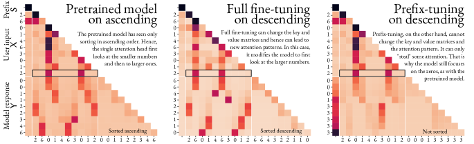
To check if prefix-tuning can learn a new task, we train a 1-layer, 1-head transformer to sort numbers into ascending order and then fine-tune it to sort in descending order. During training, the model sees random sequences of 10 digits from 0 to 7 followed by their ascending sorted order. The pretrained accuracy (fully matching the sorted sequence) is 91%. Full fine-tuning on the descending task leads to 85% test accuracy, hence full fine-tuning successfully learns the new task. However, prefix-tuning with a prefix size results in 0% accuracy, hence prefix-tuning fails to learn the new task at all.
The attention patterns in Figure 1 show why this is the case: the pretrained model learns to attend first to the smallest numbers and then to the larger ones. When fully fine-tuned, the attention patterns are reversed: they now first attend to the largest values. However, following Section 4, prefix-tuning cannot change the attention pattern over the input sequence and will still attend to the smallest values. Therefore, prefix-tuning indeed cannot learn a new task if it requires new attention patterns.
| Accuracy on: | ||||
|---|---|---|---|---|
| Pretrained | 2513% | 2512% | 2411% | 227% |
| Prefix-tune on | 95 2% | 0 0% | 0 0% | 00% |
| Prefix-tune on | 0 0% | 90 3% | 1 1% | 11% |
| Prefix-tune on | 0 0% | 1 3% | 95 6% | 01% |
| Prefix-tune on | 0 0% | 0 0% | 1 2% | 985% |
Prefix-tuning can elicit a skill from the pretrained model.
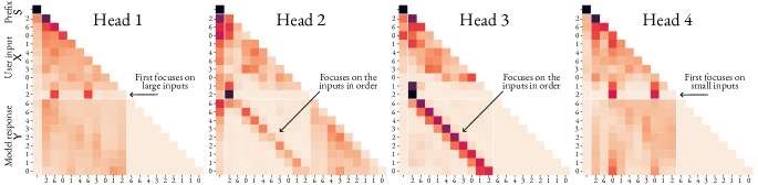
The second part of our hypothesis was that prefix-tuning can elicit latent skills in the pretrained model. To test that, we pretrain a 1-layer, 4-head model with solutions sorted in ascending () or descending () order, or adding one () or two () to each element of the input sequence. Each solution is shown with 25% probability. The model has no indication of what the task is, hence, it assigns equal probability to all tasks, as shown in the first row in Table 2. Full fine-tuning for each task naturally results in high accuracy. However, prefix-tuning can also reach very high accuracy for all tasks: above 90%. Compared to the previous case, prefix-tuning is more successful here because the pretrained model contains the attention mechanisms for solving the four tasks, as shown in Figure 2.
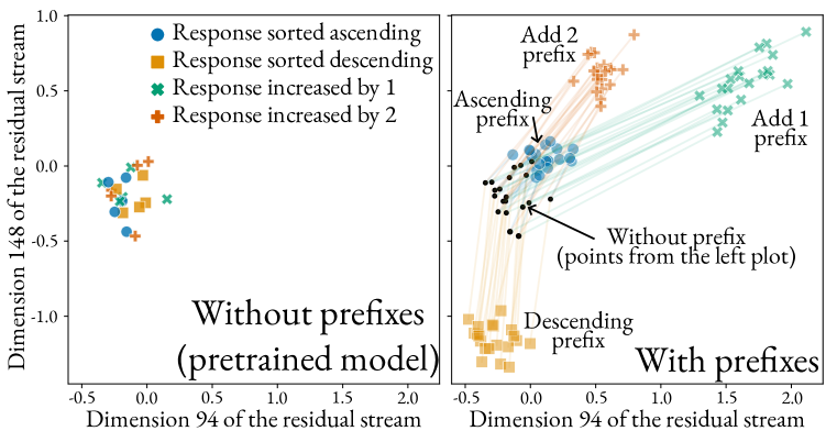
If all a prefix does is bias the attention layer activations, how can it steer the model to collapse its distribution onto one task? This is likely due to the attention block solving all tasks in parallel and placing their solutions in different subspaces of the residual stream (intermediate representation, Elhage et al., 2021). As the MLP needs to select one solution to generate, a further indicator on the selected task (or lack of selection thereof) should also be represented. The bias induced by the prefix then acts on this “selection subspace” to nudge the MLP to select the desired solution.
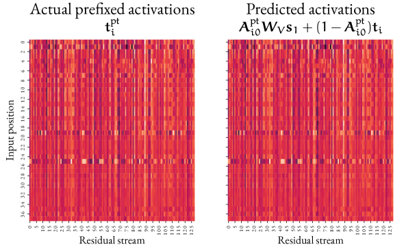
This can be be clearly seen from the activations of the attention layer at the last input position (). This is the position where the task selection happens as the first output element fully describes the task. Figure 3 shows plots of randomly selected dimensions of the residual stream with and without a prefix. The attention block activations of the pretrained model (without prefix) show no correlation with the output it is about to generate, demonstrating that the choice of completion is indeed random and is not determined by the activation block. However, the prefix-tuned activations for the same inputs are clustered as a result of the prefix-induced bias. This shows that the bias induced by the prefix acts as a “task selector” of the subspace of the residual stream specializing in the desired task.
Prefix-tuning can combine knowledge from pretraining tasks to solve new tasks.
Prefix-tuning eliciting one type of completion learned in pretraining starts to explain its practical utility. Still, prefix-tuning seems to be successful also at tasks that the pretrained model has not seen. As we showed above, a model trained to sort in one order cannot be prefix-tuned to sort in the other. Then how is it possible for prefix-tuning to learn a new task? We posit that this can happen, as long as the “skill” required to solve the new task is a combination of “skills” the pretrained model has seen.
| Accuracy on: | ||||||
|---|---|---|---|---|---|---|
| Pretrained | 17% | 23% | 34% | 25% | 0% | 0% |
| Prefix-tune on | 100% | 0% | 0% | 0% | 0% | 0% |
| Prefix-tune on | 0% | 100% | 0% | 0% | 0% | 0% |
| Prefix-tune on | 0% | 0% | 100% | 0% | 0% | 0% |
| Prefix-tune on | 0% | 0% | 0% | 100% | 0% | 0% |
| Prefix-tune on | 0% | 0% | 0% | 0% | 93% | 0% |
| Prefix-tune on | 0% | 0% | 0% | 0% | 0% | 1% |
We test this by pretraining a 40-layer 4-head model with the same four tasks. We prefix-tune () for two new tasks: incrementing the ascending sorted sequence () and double histogram (mapping each element to the number of elements in the sequence with the same value, ). The pretrained model has not seen either task. Prefix-tuning results in 93% accuracy for which is a combination of the and pretraining tasks and just 1% for the task which requires different skills: finding other instances of the same token and counting. Note that is not a hard task: it requires 2 layers and 2 heads to be solved exactly (Weiss et al., 2021). Therefore, prefix-tuning is can indeed combine skills that the model has learned in order to solve a novel task but cannot learn a completely new task requiring new skills.
6 Effects of prefix-tuning beyond the single attention layer
Section 4 focused exclusively on a single attention layer. However, even if a prefix can only induce a bias on its output, this bias, when passed through the following MLP and subsequent attention layers, can exhibit increasingly complex behaviors. While it is not immediately obvious that the limitations discussed above translate to deeper networks, we provide evidence to this end. Section 6.1 shows that a prefix can change the attention pattern of the following attention layer but only in a linear fashion while full fine-tuning can also enact bilinear effects. Section 6.2 shows that while prefix-tuning can be thought of as neural network training, the representational capacity of the resulting architecture is severely limited. Therefore, prefix-tuning appears to be less expressive than full fine-tuning, even when both methods are given the same number of learnable parameters.
6.1 Prefix-tuning can change the attention, albeit the one of the next layer
Let us examine how the prefix of one attention layer affects the following attention layer. For simplicity, assume there is no MLP between the attention layers, residual connections or layer norms: the output of the first is the input of the second. The pretrained outputs are , resulting in the second layer attention . Here is the pre-softmax attention, i.e., . For prefix-tuning we then have:
|
|
The presence of shows that the prefix of layer 1 can change the attention pattern of the following layer. This change is content-specific: the second and the third terms depend on the inputs, hence a simple bias can affect the attention when passed through MLPs and further attention blocks. Compare with Equation 6, which showed a prefix cannot change the attention of the same layer.
Still, even considering this cross-layer effect, prefix-tuning is more limited in its expressiveness than full fine-tuning. While the second and the third terms are input-dependent, each depends on one input position only. The prefix does not change the bilinear dependency on both the query and key. This is something that the full fine-tuning can achieve: .
6.2 Expressivity of prefix-tuning across deeper models
We considered the effect of the presence of the prefix in the first attention layer on the attention of the second. However, the effects become more complex as one adds more attention attention layers. We also ignored the MLPs between, but in practice they can play an important role. Here, instead, we analyse prefix-tuning as learning a neural network. We argue that while the resulting architecture includes both linear operation and non-linear activations, the structure is unlikely to learn efficiently.
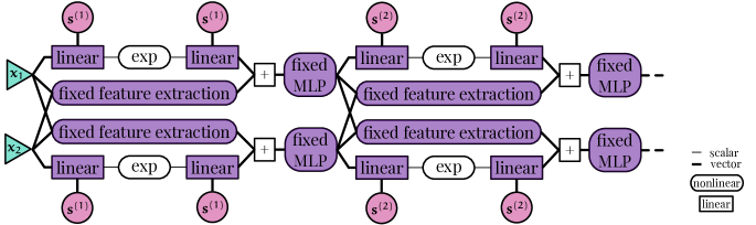
For simplicity, we will consider two inputs and and a single prefix . The output of the attention head, parameterized by is then:
| (8) | ||||
where we have omitted the factors and have folded the softmax normalization into and . The layer inputs, pretrained parameters and the learnable parameters are correspondingly highlighted. The attention head is clearly a non-linear operation. However, the learnable parameter participates only in the left term. It interacts with only one of the inputs at a time and only by computing a single scalar value . As we discussed above, the interaction between and is non-trainable and can be thought as a hard-coded feature extraction. Each of the outputs is then passed to a pretrained MLP which can be thought of as an activation function. This would be a multivariate activation function, which while unusual in the contemporary practice has been studied before (Solazzi and Uncini, 2004). Figure 4 illustrates the computation graph of the resulting neural network and shows that the only learnable interaction between the inputs is indirect. Therefore, prefix-tuning can be considered as learning a neural network where the only interaction between the inputs happens via non-learnable residual connections. Nevertheless, the alternating linear and nonlinear operations are reminiscent of the standard neural network architecture and their universal approximation properties (Hassoun, 1995). That begs the question if the prefix-tuning architecture can be an universal approximator and whether it would be a parameter-efficient one.
An example of prefix-tuning failing to be an universal approximator.
While we leave the formal analysis of the representational capacity of prefix-tuning as future work, we provide an example of pretrained parameters for which the architecture is not a universal approximator. As can be seen in Figure 4, all information must pass through the non-learnable MLPs. Thus, if the MLPs destroy all input information, there is no value for the prefixes that can change that fact. The MLPs can destroy all information, if, e.g., one of their linear layers has a zero weight matrix. While this is unlikely to be learned with typical pretraining, this demonstrates that if prefix-tuning could be a universal approximator, that would pose specific requirements on the pretrained MLPs and it is not clear whether pretraining would satisfy these requirements.
Even if prefix-tuning could be an universal approximator, it would not be parameter-efficient.
Whether prefix-tuning is an universal approximator is not of practical relevance as even if it was, it would be much less parameter-efficient than other comparable approaches. While Equation 8 and Figure 4 already hint at that, we designed an experiment to this end. Recall that our pretrained model in Section 5 failed to learn the double histogram task () as it required novel attention patterns. A rank-1 Low Rank Adaptation (LoRA, Hu et al., 2021) applied only to the MLPs in a 4-layer 4-head model pretrained in the exact same way results in 92% accuracy on the task. The number of parameters for the LoRA fine-tuning is exactly the same as for a prefix of size 12. However, as can be expected from the results in Section 5, training this prefix results in 0% accuracy. Therefore, prefix-tuning fails to learn a task that LoRA with the same number of parameters can learn.
In conclusion, while prefix-tuning, prompting, soft prompting and in-context learning have complex effects in deeper models, the interaction of the learnable parameters and the model inputs likely still results in very limited expressiveness. In particular, we demonstrated that LoRA can be used to learn a completely new task while prefix-tuning with the exact same number of parameters cannot.
7 Discussion and related works
Understanding fine-tuning and prefix-tuning.
Prior works show that prefixes have low intrinsic dimension allowing transfer to similar tasks and initialization of prefixes for new tasks (Qin et al., 2021; Su et al., 2022; Zhong et al., 2022; Wang et al., 2022b; Zheng et al., 2023). In this work, we offered theoretical insights into their results: this subspace is the span of the prefix-induced bias. Another line of work shows that skills can be localized in the parameter space of pretrained models (Wang et al., 2022a; Panigrahi et al., 2023). Here, we showed that it is also possible to identify subspaces of the residual stream corresponding to individual tasks and select them via prefix-tuning.
Prompting and in-context learning.
Prompting and in-context learning are a special case of prefix-tuning. Therefore, the limitations and mechanisms discussed in this work apply to prompting as well: prompts cannot change the distribution of attention of the first attention layer over the content following it and can only induce a bias on the output of this layer (Section 4). Even considering the cross-layer effects, a prompt is strictly less expressive than full fine-tuning (Section 6) and prompting is unlikely to enable the model to solve a completely new task. Our theory thus explains why Kossen et al. (2023) observed that in-context examples cannot overcome pre-training skills.
While context-based fine-tuning approaches cannot learn arbitrary new tasks, as shown in Section 5, they can leverage pre-trained skills. For instance, transformers can learn linear models in-context by mimicking gradient descent (Von Oswald et al., 2023) or by approximating matrix inversion (Akyürek et al., 2022). This is consistent with our theory: the prediction updates are enacted as biases in the activations of the attention block. Hence, despite the limitations discussed in this work, context-based methods can result in powerful fine-tuning if the pretrained model has “transferable skills” such as algorithmic fundamentals. Still, there are non-algorithmic applications where our theory predicts that in-context learning will fail, for example, translating to a language that the model has never seen before, even if large number of translation pairs are provided in-context.
Implications for catastrophic forgetting and model alignment.
The lack of expressiveness of context-based fine-tuning can be a feature: desirable properties will be maintained. Full fine-tuning can result in catastrophic forgetting (He et al., 2021b; Luo et al., 2023; Mukhoti et al., 2023). Our theory shows that context-based methods will not destroy pretrained skills. Model alignment poses the reverse problem: ensuring that the model cannot pick up undesirable skills during fine-tuning. Our results show that prompting and prefix-tuning cannot steer the model towards new adversarial behaviors. Hence, the recent successes in adversarial prompting (Zou et al., 2023) indicate that current model alignment methods just mask the undesirable skills rather than removing them.
Implications for model interpretability.
An open question for language model interpretability is whether attention is sufficient for explainability (Jain and Wallace, 2019; Wiegreffe and Pinter, 2019). Section 5 points toward the negative: by interfering in the output of the attention layer with the bias induced by a prefix, we can change the behavior of the model, without changing its attention. On the flip side, prefix-tuning can be used to understand what “skills” a model has: if prefix-tuning for a task fails, then the model likely lacks one of the key “skills” for that task.
Limitations.
The present analysis is largely limited to prefixing with prompts, soft prompts and for prefix-tuning. While our theoretical results hold for suffix-tuning, they do not necessarily apply to suffixing with prompts or soft prompts. That is because the deeper representations for prompt and soft prompt suffixes would depend on the previous positions. This does not apply to suffix-tuning as it fixes all intermediate representations. Therefore, whether suffixing is more expressive than prefixing remains an open question. Separately, while we provided evidence towards context-based fine-tuning methods being parameter inefficient learners, the formal analysis of the conditions under which they may be universal approximators remain an open question. Finally, we mostly considered simple toy problems. In practice, however, language models are pretrained with very large datasets and can pick up very complex behaviors. Hence, the extent to which the limitations we demonstrated apply to large-scale pretrained transformers also remains for future work.
8 Conclusion
This paper formally showed that fine-tuning techniques working in embedding space, such as soft prompting and prefix-tuning, are strictly more expressive than prompting which operates in the discrete token space. However, we then demonstrated that despite this larger expressivity, prefix-tuning suffers from structural limitations that prevent it from learning new attention patterns. As a result, it can only bias the output of the attention layer in a direction from a subspace of rank equal to the size of the prefix. We showed that this results in practical limitations by constructing minimal transformers where prefix tuning fails to solve a simple task. This result seems to be at odds with the empirical success of prefix-tuning. We provided explanations towards that. First, we showed that prefix-tuning can easily elicit a skill the pretrained model already has and can even learn a new task, if it has picked up the skills to solve it during pretraining. Second, we showed that the effect of the prefix-induced bias is more complicated and powerful when combined with downstream non-linear operations. However, it appears to be still strictly less expressive than full fine-tuning.
Reproducibility statement
In order to facilitate the reproduction of our empirical results, validating our theoretical results, and further studying the properties of context-based fine-tuning, we release all our code and resources used in this work. Furthermore, in Appendix A we offer explicit constructions of transformers with the properties discussed in Section 3. We also provide Python implementations of these constructions that validate their correctness.
Acknowledgements
This work is supported by a UKRI grant Turing AI Fellowship (EP/W002981/1) and the EPSRC Centre for Doctoral Training in Autonomous Intelligent Machines and Systems (EP/S024050/1). AB has received funding from the Amazon Research Awards. We also thank the Royal Academy of Engineering and FiveAI.
References
- Akyürek et al. (2022) Ekin Akyürek, Dale Schuurmans, Jacob Andreas, Tengyu Ma, and Denny Zhou. 2022. What learning algorithm is in-context learning? Investigations with linear models. In International Conference on Learning Representations.
- Bai et al. (2023) Jiaqi Bai, Zhao Yan, Jian Yang, Xinnian Liang, Hongcheng Guo, and Zhoujun Li. 2023. Knowprefix-tuning: A two-stage prefix-tuning framework for knowledge-grounded dialogue generation. arXiv preprint arXiv:2306.15430.
- Brown et al. (2020) Tom Brown, Benjamin Mann, Nick Ryder, Melanie Subbiah, Jared D Kaplan, Prafulla Dhariwal, Arvind Neelakantan, Pranav Shyam, Girish Sastry, Amanda Askell, et al. 2020. Language models are few-shot learners. Advances in Neural Information Processing Systems.
- Choi and Lee (2023) YunSeok Choi and Jee-Hyong Lee. 2023. CodePrompt: Task-agnostic prefix tuning for program and language generation. In Findings of the Association for Computational Linguistics: ACL 2023.
- Devlin et al. (2019) Jacob Devlin, Ming-Wei Chang, Kenton Lee, and Kristina Toutanova. 2019. BERT: Pre-training of deep bidirectional transformers for language understanding. In Proceedings of the 2019 Conference of the North American Chapter of the Association for Computational Linguistics: Human Language Technologies, Volume 1 (Long and Short Papers).
- Elhage et al. (2021) Nelson Elhage, Neel Nanda, Catherine Olsson, Tom Henighan, Nicholas Joseph, Ben Mann, Amanda Askell, Yuntao Bai, Anna Chen, Tom Conerly, Nova DasSarma, Dawn Drain, Deep Ganguli, Zac Hatfield-Dodds, Danny Hernandez, Andy Jones, Jackson Kernion, Liane Lovitt, Kamal Ndousse, Dario Amodei, Tom Brown, Jack Clark, Jared Kaplan, Sam McCandlish, and Chris Olah. 2021. A mathematical framework for transformer circuits. Transformer Circuits Thread.
- Hambardzumyan et al. (2021) Karen Hambardzumyan, Hrant Khachatrian, and Jonathan May. 2021. WARP: Word-level Adversarial ReProgramming. In Proceedings of the 59th Annual Meeting of the Association for Computational Linguistics and the 11th International Joint Conference on Natural Language Processing (Volume 1: Long Papers).
- Hassoun (1995) Mohamad H Hassoun. 1995. Fundamentals of artificial neural networks. MIT press.
- He et al. (2021a) Junxian He, Chunting Zhou, Xuezhe Ma, Taylor Berg-Kirkpatrick, and Graham Neubig. 2021a. Towards a unified view of parameter-efficient transfer learning. In International Conference on Learning Representations.
- He et al. (2021b) Tianxing He, Jun Liu, Kyunghyun Cho, Myle Ott, Bing Liu, James Glass, and Fuchun Peng. 2021b. Analyzing the forgetting problem in pretrain-finetuning of open-domain dialogue response models. In Proceedings of the 16th Conference of the European Chapter of the Association for Computational Linguistics: Main Volume.
- Houlsby et al. (2019) Neil Houlsby, Andrei Giurgiu, Stanislaw Jastrzebski, Bruna Morrone, Quentin De Laroussilhe, Andrea Gesmundo, Mona Attariyan, and Sylvain Gelly. 2019. Parameter-efficient transfer learning for NLP. In International Conference on Machine Learning.
- Hu et al. (2021) Edward J Hu, Yelong Shen, Phillip Wallis, Zeyuan Allen-Zhu, Yuanzhi Li, Shean Wang, Lu Wang, and Weizhu Chen. 2021. LoRA: Low-rank adaptation of large language models. In International Conference on Learning Representations.
- Hu et al. (2023) Zhiqiang Hu, Yihuai Lan, Lei Wang, Wanyu Xu, Ee-Peng Lim, Roy Ka-Wei Lee, Lidong Bing, and Soujanya Poria. 2023. LLM-Adapters: An adapter family for parameter-efficient fine-tuning of large language models. arXiv preprint arXiv:2304.01933.
- Jain and Wallace (2019) Sarthak Jain and Byron C. Wallace. 2019. Attention is not explanation. In Proceedings of the 2019 Conference of the North American Chapter of the Association for Computational Linguistics: Human Language Technologies, Volume 1 (Long and Short Papers).
- Kaplan et al. (2020) Jared Kaplan, Sam McCandlish, Tom Henighan, Tom B Brown, Benjamin Chess, Rewon Child, Scott Gray, Alec Radford, Jeffrey Wu, and Dario Amodei. 2020. Scaling laws for neural language models. arXiv preprint arXiv:2001.08361.
- Karpathy (2020) Andrej Karpathy. 2020. minGPT GitHub Repository.
- Kojima et al. (2022) Takeshi Kojima, Shixiang Shane Gu, Machel Reid, Yutaka Matsuo, and Yusuke Iwasawa. 2022. Large language models are zero-shot reasoners. Advances in Neural Information Processing Systems.
- Kossen et al. (2023) Jannik Kossen, Tom Rainforth, and Yarin Gal. 2023. In-context learning in large language models learns label relationships but is not conventional learning. arXiv preprint arXiv:2307.12375.
- La Malfa et al. (2023) Emanuele La Malfa, Aleksandar Petrov, Christoph Weinhuber, Simon Frieder, Ryan Burnell, Anthony G. Cohn, Nigel Shadbolt, and Michael Wooldridge. 2023. The ARRT of Language-Models-as-a-Service: Overview of a new paradigm and its challenges. arXiv preprint arXiv:2309.16573.
- Lester et al. (2021) Brian Lester, Rami Al-Rfou, and Noah Constant. 2021. The power of scale for parameter-efficient prompt tuning. In Proceedings of the 2021 Conference on Empirical Methods in Natural Language Processing.
- Li and Liang (2021) Xiang Lisa Li and Percy Liang. 2021. Prefix-Tuning: Optimizing continuous prompts for generation. In Proceedings of the 59th Annual Meeting of the Association for Computational Linguistics and the 11th International Joint Conference on Natural Language Processing (Volume 1: Long Papers).
- Lialin et al. (2023) Vladislav Lialin, Vijeta Deshpande, and Anna Rumshisky. 2023. Scaling down to scale up: A guide to parameter-efficient fine-tuning. arXiv preprint arXiv:2303.15647.
- Liu et al. (2023) Pengfei Liu, Weizhe Yuan, Jinlan Fu, Zhengbao Jiang, Hiroaki Hayashi, and Graham Neubig. 2023. Pre-train, prompt, and predict: A systematic survey of prompting methods in natural language processing. ACM Computing Surveys.
- Liu et al. (2022) Xiao Liu, Kaixuan Ji, Yicheng Fu, Weng Tam, Zhengxiao Du, Zhilin Yang, and Jie Tang. 2022. P-Tuning: Prompt tuning can be comparable to fine-tuning across scales and tasks. In Proceedings of the 60th Annual Meeting of the Association for Computational Linguistics (Volume 2: Short Papers).
- Luo et al. (2023) Yun Luo, Zhen Yang, Fandong Meng, Yafu Li, Jie Zhou, and Yue Zhang. 2023. An empirical study of catastrophic forgetting in large language models during continual fine-tuning. arXiv preprint arXiv:2308.08747.
- Min et al. (2021) Bonan Min, Hayley Ross, Elior Sulem, Amir Pouran Ben Veyseh, Thien Huu Nguyen, Oscar Sainz, Eneko Agirre, Ilana Heintz, and Dan Roth. 2021. Recent advances in natural language processing via large pre-trained language models: A survey. ACM Computing Surveys.
- Mukhoti et al. (2023) Jishnu Mukhoti, Yarin Gal, Philip H. S. Torr, and Puneet K. Dokania. 2023. Fine-tuning can cripple your foundation model; preserving features may be the solution. arXiv preprint arXiv:2308.13320.
- Nan et al. (2021) Linyong Nan, Dragomir Radev, Rui Zhang, Amrit Rau, Abhinand Sivaprasad, Chiachun Hsieh, Xiangru Tang, Aadit Vyas, Neha Verma, Pranav Krishna, Yangxiaokang Liu, Nadia Irwanto, Jessica Pan, Faiaz Rahman, Ahmad Zaidi, Mutethia Mutuma, Yasin Tarabar, Ankit Gupta, Tao Yu, Yi Chern Tan, Xi Victoria Lin, Caiming Xiong, Richard Socher, and Nazneen Fatema Rajani. 2021. DART: Open-domain structured data record to text generation. In Proceedings of the 2021 Conference of the North American Chapter of the Association for Computational Linguistics: Human Language Technologies.
- Ouyang et al. (2023) Yawen Ouyang, Yongchang Cao, Yuan Gao, Zhen Wu, Jianbing Zhang, and Xinyu Dai. 2023. On prefix-tuning for lightweight out-of-distribution detection. In Proceedings of the 61st Annual Meeting of the Association for Computational Linguistics (Volume 1: Long Papers).
- Panigrahi et al. (2023) Abhishek Panigrahi, Nikunj Saunshi, Haoyu Zhao, and Sanjeev Arora. 2023. Task-specific skill localization in fine-tuned language models. In International Conference on Machine Learning.
- Qin and Eisner (2021) Guanghui Qin and Jason Eisner. 2021. Learning how to ask: Querying LMs with mixtures of soft prompts. In Proceedings of the 2021 Conference of the North American Chapter of the Association for Computational Linguistics: Human Language Technologies.
- Qin et al. (2021) Yujia Qin, Xiaozhi Wang, Yusheng Su, Yankai Lin, Ning Ding, Jing Yi, Weize Chen, Zhiyuan Liu, Juanzi Li, Lei Hou, et al. 2021. Exploring universal intrinsic task subspace via prompt tuning. arXiv preprint arXiv:2110.07867.
- Radford et al. (2019) Alec Radford, Jeff Wu, Rewon Child, David Luan, Dario Amodei, and Ilya Sutskever. 2019. Language models are unsupervised multitask learners.
- Rae et al. (2021) Jack W. Rae, Sebastian Borgeaud, Trevor Cai, Katie Millican, Jordan Hoffmann, Francis Song, John Aslanides, Sarah Henderson, Roman Ring, et al. 2021. Scaling language models: Methods, analysis & insights from training Gopher.
- Rebuffi et al. (2017) Sylvestre-Alvise Rebuffi, Hakan Bilen, and Andrea Vedaldi. 2017. Learning multiple visual domains with residual adapters. In Advances in Neural Information Processing Systems.
- Reynolds and McDonell (2021) Laria Reynolds and Kyle McDonell. 2021. Prompt programming for large language models: Beyond the few-shot paradigm. In Extended Abstracts of the 2021 CHI Conference on Human Factors in Computing Systems.
- Saravia et al. (2018) Elvis Saravia, Hsien-Chi Toby Liu, Yen-Hao Huang, Junlin Wu, and Yi-Shin Chen. 2018. CARER: Contextualized affect representations for emotion recognition. In Proceedings of the 2018 Conference on Empirical Methods in Natural Language Processing.
- Shin et al. (2020) Taylor Shin, Yasaman Razeghi, Robert L. Logan IV, Eric Wallace, and Sameer Singh. 2020. AutoPrompt: Eliciting knowledge from language models with automatically generated prompts. In Proceedings of the 2020 Conference on Empirical Methods in Natural Language Processing (EMNLP).
- Solazzi and Uncini (2004) Mirko Solazzi and Aurelio Uncini. 2004. Regularising neural networks using flexible multivariate activation function. Neural Networks, 17(2):247–260.
- Su et al. (2022) Yusheng Su, Xiaozhi Wang, Yujia Qin, Chi-Min Chan, Yankai Lin, Huadong Wang, Kaiyue Wen, Zhiyuan Liu, Peng Li, Juanzi Li, Lei Hou, Maosong Sun, and Jie Zhou. 2022. On transferability of prompt tuning for natural language processing. In Proceedings of the 2022 Conference of the North American Chapter of the Association for Computational Linguistics: Human Language Technologies.
- Sun et al. (2022) Tianxiang Sun, Yunfan Shao, Hong Qian, Xuanjing Huang, and Xipeng Qiu. 2022. Black-box tuning for language-model-as-a-service. In International Conference on Machine Learning.
- Touvron et al. (2023) Hugo Touvron, Thibaut Lavril, Gautier Izacard, Xavier Martinet, Marie-Anne Lachaux, Timothée Lacroix, Baptiste Rozière, Naman Goyal, Eric Hambro, Faisal Azhar, et al. 2023. LLaMA: Open and efficient foundation language models. arXiv preprint arXiv:2302.13971.
- Vaswani et al. (2017) Ashish Vaswani, Noam Shazeer, Niki Parmar, Jakob Uszkoreit, Llion Jones, Aidan N. Gomez, Lukasz Kaiser, and Illia Polosukhin. 2017. Attention is all you need. In Advances in Neural Information Processing Systems.
- Von Oswald et al. (2023) Johannes Von Oswald, Eyvind Niklasson, Ettore Randazzo, Joao Sacramento, Alexander Mordvintsev, Andrey Zhmoginov, and Max Vladymyrov. 2023. Transformers learn in-context by gradient descent. In International Conference on Machine Learning.
- Vu et al. (2022) Tu Vu, Brian Lester, Noah Constant, Rami Al-Rfou’, and Daniel Cer. 2022. SPoT: Better frozen model adaptation through soft prompt transfer. In Proceedings of the 60th Annual Meeting of the Association for Computational Linguistics (Volume 1: Long Papers).
- Wang et al. (2022a) Xiaozhi Wang, Kaiyue Wen, Zhengyan Zhang, Lei Hou, Zhiyuan Liu, and Juanzi Li. 2022a. Finding skill neurons in pre-trained transformer-based language models. In Proceedings of the 2022 Conference on Empirical Methods in Natural Language Processing.
- Wang et al. (2022b) Zhen Wang, Rameswar Panda, Leonid Karlinsky, Rogerio Feris, Huan Sun, and Yoon Kim. 2022b. Multitask prompt tuning enables parameter-efficient transfer learning. In International Conference on Learning Representations.
- Wei et al. (2021) Jason Wei, Maarten Bosma, Vincent Zhao, Kelvin Guu, Adams Wei Yu, Brian Lester, Nan Du, Andrew M Dai, and Quoc V Le. 2021. Finetuned language models are zero-shot learners. In International Conference on Learning Representations.
- Weiss et al. (2021) Gail Weiss, Yoav Goldberg, and Eran Yahav. 2021. Thinking like transformers. In International Conference on Machine Learning.
- Wiegreffe and Pinter (2019) Sarah Wiegreffe and Yuval Pinter. 2019. Attention is not not explanation. In Proceedings of the 2019 Conference on Empirical Methods in Natural Language Processing and the 9th International Joint Conference on Natural Language Processing (EMNLP-IJCNLP).
- Wu and Shi (2022) Hui Wu and Xiaodong Shi. 2022. Adversarial soft prompt tuning for cross-domain sentiment analysis. In Proceedings of the 60th Annual Meeting of the Association for Computational Linguistics (Volume 1: Long Papers).
- Zheng et al. (2023) Yuanhang Zheng, Zhixing Tan, Peng Li, and Yang Liu. 2023. Black-box prompt tuning with subspace learning. arXiv preprint arXiv:2305.03518.
- Zhong et al. (2022) Qihuang Zhong, Liang Ding, Juhua Liu, Bo Du, and Dacheng Tao. 2022. PANDA: Prompt transfer meets knowledge distillation for efficient model adaptation. arXiv preprint arXiv:2208.10160.
- Zou et al. (2023) Andy Zou, Zifan Wang, J Zico Kolter, and Matt Fredrikson. 2023. Universal and transferable adversarial attacks on aligned language models. arXiv preprint arXiv:2307.15043.
Appendix A Constructing transformers that utilize the capacity of the embedding space
A.1 Unconditional generation for a single virtual token
This section provides an explicit construction of a transformer with the properties described in Theorem 1. The goal is to construct a transformer that, by varying the choice of the virtual token, can generate any sequence of tokens.
First, we need to specify how we encode the target sequence into the virtual token . We chose the size of the embedding (and hence of ) to be . This way, each element of can represent one position of the target sequence. We then represent the token value by discretizing each element of into levels:
Note that this means that each element of is in .
When predicting the token for the position, the transformer needs to pick the -th element of , and then decode the corresponding value as a one-hot encoding representing the -th token.
We extract the -th element of using one attention block of two heads. The fst head always looks at the first position which is our virtual token . For that purpose we create an attention head that always has if and otherwise together with a value matrix that extracts the embedding. This is achieved with
| (9) |
and a sufficiently high inverse temperature parameter .
The pos head instead extracts the one-hot encoding of the current position. This can be done with an attention head that always attends only to the current position and a value matrix that extracts the position embedding as a one-hot vector:
| (10) |
When the outputs of these two attention heads are summed, then only the element of that corresponds to the current position will be larger than 1. From Equation 2 the output at the -th position of the attention block is:
where and for .
We can extract the value of corresponding to the current position by substracting 1 from the hidden state and apply ReLU: . Now, we are left with only one non-zero entry and that’s the one corresponding to the next token. We can retain only the non-zero entry if we just sum all the entries of the hidden state with .
The final step is to map this scalar to a -dimensional vector which has its maximum value at index . This task is equivalent to designing linear functions, each attaining its maximum at one of . To construct this, we use the property of convex functions that their tangent is always under the plot of the function. Therefore, given a convex function , we construct the -th linear function to be simply the tangent of at . If we take , this results in the following linear layer:
| (11) |
Figure 5 shows the predictors for each individual token id.
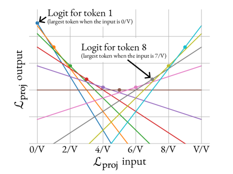
With just two attention heads and three linear layers, the transformer achieves the upper bound of unique outputs by controlling a single virtual token at its input. Note that for this construction, the choice of embedding matrix does not matter. The same transformer architecture can generate only unique outputs if we only control the first token instead. Therefore, it is indeed the case that the embedding space has exponentially more capacity for control than the token space. You can see this transformer implemented and running in practice in Section 2 of the constructions Jupyter notebook.
A.2 Conditional generation for a single virtual token ()
This section provides an explicit construction of a transformer with the properties described in Theorem 2. The goal is to construct a transformer that, by varying the choice of the virtual token, can cause the model to act as any map . In other words, by selecting the virtual token, we can fully control how the model will respond to any token the user may provide.
First, we need to specify how the map will be encoded in the virtual token . We choose the embedding size to be . Now, we can use the same encoding scheme as before, but now each element in corresponds to a different user token, rather than to a position in the generated sequence:
Therefore, the first element of designates the response if the user provides token 1, the second element is the response to the token 2, and so on.
Extracting the -th value from and decoding it can be done in a very similar way as for the unconditional case. The only difference is that instead of looking at the user input position, we look at its value. Take and .
Hence we have the following val head (only differing in the matrix from Equation 10):
We also need embedding of the first token, so we have a modified version of Equation 9:
And hence the output of this attention block at the second position would be:
Similarly to the unconditional case, only the entry of corresponding to the user token will have a value above 1 and that value would be .
We can now extract the one-hot representation of the target token using the same approach as before, just adjusting for the different hidden state size: , , and the same projection had as before (Equation 11). The final transformer is then: You can see this transformer implemented and running in practice in Section 3 of the constructions Jupyter notebook.
A.3 Conditional generation for longer responses ()
We can obtain longer responses via a simple extension. If the response length is , then we can encode the map in virtual tokens, each corresponding to one of the target positions:
For this model we would then have and .
First, we need a head that always looks at the token provided by the user, which will be at position :
In order to consume the map at the right location, we need to also look at the embedding of the token positions before the one we are trying to generate:
From here on, the decoding is exactly the same as in the case. The final transformer is then: You can see this transformer implemented and running in practice in Section 4 of the constructions Jupyter notebook.
A.4 Conditional generation for longer user inputs (, )
Finally, we consider the case when the user input X is longer. This is a bit more complicated because we need to search through a domain of size . We will only consider the case with where we would need two attention layers. A similar approach can be used to construct deeper models for . Finally, combining the strategy in the previous section for longer responses with the strategy in this section for longer user inputs allows us to construct transformers that map from arbitrary length user strings to arbitrary length responses.
In order to encode a map into a single virtual token we would need a more involved construction than before. Similarly to how we discretized each element of the virtual token in levels before, we are going to now discretize it into levels. Each one of these levels would be one of the possible maps from the second user token to the response. The first user token would be used to select the corresponding element of . Then this scalar will be “unpacked” into a new vector of elements using the first attention block. Then, the second user token will select an element from this unpacked vector, which will correspond to the target token.
We construct the virtual token as follows:
where is a map from the second user token to the response when the first token is fixed to be .
An additional change from the previous constructions is that we are going to divide the residual stream into two sections. This is in line with the theory that different parts of the residual stream specialize for different communications needs by different attention heads (Elhage et al., 2021). We will use the first half of the residual stream to extract and “unpack” the correct mapping from second token to target token, while the second half of the residual stream will be used to copy the second token value so that the second attention layer can use it to extract the target. As usual, the embedding matrix will be the identity matrix: . Finally, for convenience, we will also use a dummy zero virtual token that we will attend to when we want to not attend to anything. This results in context size with the input being
We want the output at the last position to be the target , that is:
The first attention block will have three attention heads.
As before, we want to extract the value of that corresponds to the first token the user provided () and place it in the first half of the residual stream. We want only the third position to do that, while the rest of the positions keep the first half of their residual stream with zeros. Hence we have the following fst head:
|
|
The user1 head extracts the value of the first user-provided token () and also places it in the first half of the residual stream:
|
|
And the user2 head does the same for the value of the second user-provided token (), placing it in the second half of the residual stream:
|
|
where the factor 2 is there because, as usual, the first linear layer will subtract 1 from everything in order to extract the value selected by the first token.
This linear layer looks as usual: . The result is that the first elements will be 0 except one which designates which map from second user token to output we should use, and the second elements have a one hot-encoding of the second user token. Constructing an MLP that unpacks the mapping can become quite involved so we do not provide an explicit form for it. But from the universal approximation theorems and the finiteness of the domain and range, we know that such an MLP should exist. We thus designate by unpack the MLP that decodes the first half of the residual stream to:
and keeps the second half unchanged.
And now, by using two attention heads, the second attention block extracts the value of the above vector at the position designated by the second token, in a fashion not dissimilar to all the previous cases:
And finally, with , , and the same projection had as before (Equation 11), we get the target token. The final transformer is then: You can see this transformer implemented and running in practice in Section 5 of the constructions Jupyter notebook.
Appendix B Attention distribution over the prefix
As discussed in Section 4, longer prefixes define a subspace from which the bias for the attention block is selected. For a prefix of size , that means that this subspace is -dimensional. Each of prefix position defines a basis vector for this subspace, while the attention on this position determines how much of this basis component contributes to the bias.
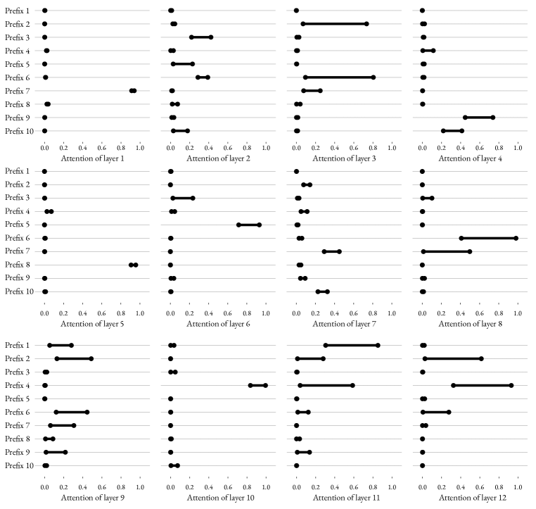
In ordered to span the whole subspace and make full use of the capacity of the prefix, should vary between 0 and 1 for different inputs. However, we observe that this does not happen in practice. Figure 8 shows the ranges of attention the different prefix positions take for the GPT-2 model (Radford et al., 2019). For layer 1, for example, the attention each prefix positions gets is almost constant hence, the effective subspace is collapsed and there is a single bias vector that’s applied to the attention layer output, regardless of the user input .
Some other layers show slightly higher variation. For example, layer 3 has three prefix positions with large variations. Therefore, the effective bias subspace is 3-dimensional and the user input governs which bias vector from this subspace will be selected.