Dynamics of an SIR epidemic model with limited medical resources, revisited and corrected

Abstract

This paper generalizes and corrects a famous paper (more than 200 citations) concerning Hopf and Bogdanov-Takens bifurcations due to L. Zhou and M. Fan, “Dynamics of an SIR epidemic model with limited medical resources revisited”, in which we discovered a significant numerical error. Importantly, unlike the paper of Zhou and Fan and several other papers which followed them, we offer a notebook where the reader may recover all the results, and also modify them for analyzing similar models. Our calculations lead to the introduction of some interesting symbolic objects, ”Groebner eliminated traces and determinants” – see (4.5), (4.6), which seem to have appeared here for the first time, and which might be of independent interest. We hope our paper might serve as yet another alarm bell regarding the importance of accompanying papers involving complicated hand computations by electronic notebooks.

Keywords:

SIR model; nonlinear force of infection; bifurcation analysis; periodic solutions; co-dimension 1 and 2 bifurcations; symbolic computing; Groebner basis.

1 Setting the problem

This work is motivated by the task of obtaining stability and bifurcation results for a “Capasso-Ruan-Wang” SIR-type epidemic model

$$\begin{cases}\mathsf{s}^{\prime}(t)=\left[b-\mu\;\mathsf{s}(t)\right]-\mathsf{s}(t)\left[\gamma_{s}+\mathsf{i}(t)N(\mathsf{i}(t))\right]+i_{s}\mathsf{i}(t)+\gamma_{r}\mathsf{r}(t),\\ \mathsf{i}^{\prime}(t)=\mathsf{i}(t)\left[\mathsf{s}(t)N(\mathsf{i}(t))-(\gamma+\mu_{i})\right]-T(\mathsf{i}(t)),\quad\gamma=i_{s}+i_{r},\mu_{i}=\mu+\delta\\ \mathsf{r}^{\prime}(t)=\gamma_{s}\mathsf{s}(t)+i_{r}\mathsf{i}(t)-{(\gamma_{r}+\mu)}\mathsf{r}(t)+T(\mathsf{i}(t)),\end{cases}$$ (1.1)

which generalizes many models studied in the last decades, including works by Capasso and Serio, Shigui Ruan, Wendy Wang, L. Zhou and M. Fan, Vyska and Gilligan, E. Avila-Vales, Pei Yu and coauthors [CS78, WR04, Wan06, ZF12, VG16, REAVGA16, PAVGA19, LHRY21, PHH21, GK22].

This model includes

• Known rates: $b,\mu,\delta,\gamma_{s}\;$ (of births, deaths, deaths due to epidemics, and vaccination).

• Three statistically estimable transition rates: $\gamma_{r},i_{r},i_{s}$ (of loss of immunity, and of recovery rates with/without immunity).

• A nonlinear correction $N(\mathsf{i})$ to the usual constant infectivity rate, introduced and studied in the influential papers by Capasso [CS78], by Liu et.al. [LHL87], and by Hethcote and Van den Driessche [HVdD91], with the purpose of capturing the psychological reaction of a population to the evolution of the epidemics (note that this type of terms is also popular in the ecology literature [SW18]).

• A nonlinear, bounded treatment $\mathbb{R}_{+}\ni\mathsf{i}\rightarrow T(\mathsf{i})\in\mathbb{R}_{+}$, which unifies two cases previously studied in the literature:

  $$T(\mathsf{i})=\begin{cases}\eta\mathsf{i}\quad 0\leq\mathsf{i}\leq\omega\\ \eta\omega\quad\mathsf{i}>\omega\end{cases}\;,\quad T(i)=\eta\frac{\mathsf{i}}{1+\mathsf{i}/\omega},\quad\eta>0,\omega>0.$$

  Note that both parametrizations have been chosen to behave as

  $$T(\mathsf{i})\approx\begin{cases}\eta{\mathsf{i}}&\mathsf{i}\approx 0\\ \eta\omega&\mathsf{i}\approx\infty\end{cases}.$$

  Here, we only consider the second case (which may be viewed as a smooth approximation of the more natural first case).

Remark 1

The vaccination rate of the susceptibles $\gamma_{s}$ is absent in the previous works. We also generalize by assuming the infected individuals may either transition to the recovery compartement at rate $i_{r}$, after successful treatment, or revert to susceptible at rate $i_{s}$, without ever becoming immune (the treatment could be partially successful, but fail to produce immunity).

Remark 2

We are using in (1.1) a unified notation scheme proposed in [AABH22, AAH22, AAB⁺21], which could be applied to any compartmental model. We propose that a linear rate of transfer from compartment $m$ to compartment $c$ be denoted by $m_{c}$, and the total linear rate out of $m$ is denoted by $\gamma_{m}$, which implies $\sum_{c}m_{c}=\gamma_{m}$ (for example the total removal rate is $\gamma_{i}=i_{s}+i_{r}$), and new infection parameters be all denoted by $\beta_{c_{1},c_{2}}$, where $c_{1}$ and $c_{2}$ are the source and destination compartments. However, simplifications will be made like $\beta_{s,i}=\beta,\gamma_{i}=\gamma$ for notations already well established traditionally.

Remark 3

Assuming $T(\mathsf{i}),N(\mathsf{i})\geq 0,T(0)=0$, implies for polynomial dynamical systems the “essential nonnegativity” of (1.1), i.e. the fact that it never leaves the nonnegative octant invariant – see [HCH10, FR00].

1.1 The purpose of bifurcation analysis

According to John Guckenheimer, Scholarpedia, 2(6):1517, the first goal of bifurcation theory is to produce parameter space maps that divide the parameter space into regions of topologically equivalent systems.

This is a very challenging process for models with many parameters, and a reasonable way to proceed is to decompose it in the following steps:

1. Fix all of the parameters except two, in a way that produces an interesting two -dimensional partition of the space of the remaining parameters into regions with different numbers of fixed points and stability properties. The determination of interesting regions requires either some symbolic knowledge of the system, or numeric continuation software ( the most well-known open-wares for the latter are Python, Julia and MatCont).

2. Identify the “corner/co-dimension 2 points” (for example, the Bogdanov-Takens points), where more than two regions meet, which may be used to organize the computations.

3. Elucidate, via time and phase-plots, the topological behavior of the dynamics in each of the regions encountered, paying special attention to bifurcations, i.e. to the topological changes which occur when crossing boundaries between regions, and notably the corners. This may be achieved by any CAS, and we have found convenient to use the Mathematica package EcoEvo – see [Kla21].

As mentioned, there is a vast literature on variations of our class of models (1.1), reviewed briefly in section 2. However, only a small part follow the three-step philosophy mentioned above, and an even smaller part mention the time-length of the computations, which has long been recognized as the essential bottleneck in the parallel disciplines of chemical reaction networks, population dynamics, ecology, etc. For some places where this point is touched on, see [PS05, MY20], which propose unifying all these disciplines under the name of computational/algebraic biology.

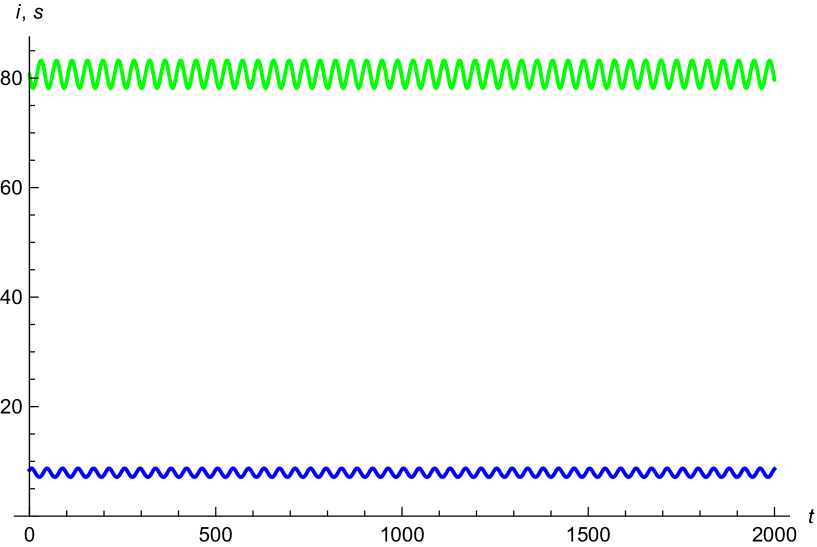
(a) $(s,i)$-time plot indicate the existence of a limit cycle surrounding $E_{2}$

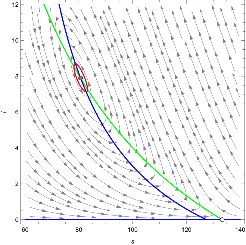
(b) $(\mathsf{s},\mathsf{i})$- phase plot. The period of the cycle is $41.6159$, and the Floquet exponents are $\left(-3.17375\times 10^{-7}\pm 9.35363\times 10^{-6}\;Im\right)$

Figure 6: Time and phase-plot corresponding to boundary $Tr(J(E_{2}))=0$ between regions II and III in Figure 2, with $\left\{\omega=6,\alpha=5.00625\right\}\Longrightarrow\mathcal{R}_{0}=1.04626>1$.

One of the results reflecting the three-step philosophy is Figure [ZF12, Fig. 6], reproduced with our notebook as Figure 2 below, which deals with the particular case $\gamma_{r}=\gamma_{s}=i_{s}=0$ of (1.1), and uses the parameter $\alpha$ of [ZF12] defined by $\alpha:=\eta\omega$.

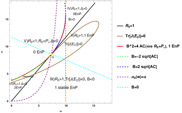
Figure 1: The original partition in [ZF12] of the $(\omega,\alpha)$ plane into regions, defined by the ${\mathcal{R}}_{0}=1,Discriminant=0,Tr\left(J_{E_{2}}\right)=0$ (other less important dotted curves from the original are included as well). The “yellow point” at which five curves seem to meet turns out to be an optical illusion, which covers an interesting seventh region, invisible at this scale.

We are building below on the results of [ZF12]. This paper is very well written; it should be mentioned however that it is written somewhat from a “I don’t need a computer/high school olympiad problem” point of view, in the sense that the authors dedicate pages to switching to new parameters and explicitizing implicit equations, which is typically unnecessary when using a computer.

Our first improvement on [ZF12] is the discovery that Figure [ZF12, Fig. 6] contains an optical illusion. Due to the choice of parameters, three important points appear superposed in the yellow point in the figure 2 (denoted by $e$ in [ZF12]), where it appears wrongly that five curves meet.

This is corrected in our pictures below 2, 4. Note that producing this small modification translated into months of work for us, due to the omission by [ZF12] to provide their notebooks.

1.2 The importance of computational aspects in the study of dynamical systems

It may be argued that nowadays, all papers written on applied dynamic models should be approached from a computational science point of view. Indeed, the fundamental problems of determining the number of fixed points and limit cycles, and of identifying bifurcations (Hopf, saddle-node, Bogdanov-Takens), etc, reduce all to the solution of polynomial systems of equalities or inequalities. Now the modern tools for tackling symbolically such problems come from algebraic geometry (like Groebner bases).

Sometimes, CAS’s (which use Groebner bases for solving) solve our problems immediately, sometimes one needs to “twist” the notebook before reaching a result, and sometimes one needs to plug in a numeric condition (possibly with parameters determined by physical experimentation). In all these cases, the notebook becomes a crucial part of a paper.

The remarkable opportunity we have nowadays of being able to accompany our pencil calculations with electronic notebooks was emphasized already 30 years ago in papers like “Electronic documents give reproducible research a new meaning” [CK92] – see also [BD95, Don10]. Following the efforts of numerous people, lots of progress has been achieved in this direction, as witnessed in particular by the existence of the platform GitHub.

1.3 A critic of the mathematical epidemiology bifurcations literature

We believe that a great part of the mathematical epidemiology literature suffers today from two draw-backs.

1. The major one is the lack of “electronic reproducibility”, i.e. of notebooks made public. Here, we provide electronic notebooks for the papers cited above, where the reader may recover the results, and also modify them as he pleases, for analyzing similar models. We believe that electronic reproducibility in the above sense should be the norm in the field of mathematical biology.

2. A second draw-back in our opinion is the focus on particular cases, furthermore studied under simplifying assumptions, which are often difficult to justify epidemiologically, like assuming $0$ deaths or eternal immunity. It seems sometimes that the justification of the simplifying assumptions is to allow a “solution by hand”, in the spirit of “mathematics olympiad problems”. Solving particular cases may of course be quite useful pedagogically, but is not efficient. For just one of many examples where symbolic computing beats easily hand computations, note that the “mathematics olympiad literature” restricts itself often to polynomials of order $2$, to be able to use their elementary discriminant formula, which is of course unnecessary nowadays. We believe that mathematical epidemiology could be better served by relying more heavily on modern symbolic computation. As another benefit, from this point of view there is no need to dedicate separate papers to each particular case of general models like (1.1). A more natural approach would be to study unified general cases symbolically as far as possible (until encountering time constraints), pinpointing how far can one push symbolics, and turn to symbolic or numeric particular cases only subsequently.

   Below, we investigate our model at two levels:

   1. The general one in (3.1), for which we may already provide simple information, like $R_{0}$, and the maximum possible number of fixed points.

   2. The particular case (4.1), for which we are able to provide bifurcation results as well.

      We believe that the traditional paradigm of one model, one paper doesn’t suit well mathematical epidemiology, where the interesting model for epidemiologists is always quite general, but mathematicians are only able to solve completely just particular cases (which may be uninteresting for epidemiologists).

Contributions. Our motivation for revisiting the bifurcation work of [ZF12] was the desire to accomplish the task of providing an electronic notebook, which may eventually be easily modified for studying variations of similar models. This quite non-trivial task required in particular pinpointing the “symbolic-numeric boundary” for this problem, which turned out to be the computation of the trace at the stable endemic point $E_{2}$. This calculation was first achieved in numeric instances, but finally also symbolically by Mathematica, and lead to the introduction of some interesting symbolic objects, ”Groebner eliminated traces and determinants” – see (4.5), (4.6), which seem to have appeared here for the first time.

Contents. Our paper starts in section 2 highlights of previous literature concerning the SIRS model with nonlinear force of infection and treatment. It then formulates in section 3, (3.1), a general epidemic model, for which $R_{0}$ and the “scalarization” of the fixed point system are easily achieved. The analysis of the simplest particular case $\gamma_{r}=\gamma_{s}=i_{s}=0$, studied in [ZF12, GK22], is then revisited and corrected in Section 4. Section 4.2 introduces the interesting ”Groebner eliminated traces and determinants” (4.5), (4.6), which turn out useful in the determination of Bogdanov-Takens bifurcations. Sections 4.3, 4.4 complete aspects missing in the original papers concerning the two-parameter bifurcation diagram and the important “corners where several regions meet”. Last but not least, our paper is accompanied by electronic notebooks supporting the results.

2 A review of the literature on the SIRS model with nonlinear force of infection and treatment

The epidemic model (1.1) is inspired firstly by the pioneering work of Capasso and Serio [CS78] (having currently 1100 citations), which propose to capture in $N(\mathsf{i})$ psychological (smooth) self regulating adaptations of the population to the epidemics. Further works of Liu, Hethcote, Levin and Iwasa [LLI86, LHL87] on power type interactions $\mathsf{s}\mathsf{i}N(\mathsf{i})\sim\mathsf{s}\mathsf{i}^{p}$ suggest adopting a classification of forces of infection in three cases, $p<1,p=1,p>1$. Subsequently, researchers have turned to studying fractional forms like $\mathsf{s}\mathsf{i}N(\mathsf{i})=\mathsf{s}\frac{\beta\mathsf{i}^{\epsilon}}{1+\xi_{1}\mathsf{i}+\xi_{2}\mathsf{i}^{2}},\;\epsilon\in\mathbb{N}$. We recommend the choice $2$ for the degree of the denominator, since this allows, by varying $\epsilon$, for including all the three cases of [LLI86, LHL87]. The corresponding cases become now:

1. $\epsilon=1$ (“non-monotone case”), see for example [PHH21],

2. $\epsilon\geq 3$ (“ultimately increasing”), see for example [LL14], and

3. $\epsilon=2$ – see [RW03, THRZ08].

In this paper, we will only consider the case $\epsilon=1$ from now on.

The pioneering papers of Wendy Wang and Shigui Ruan [WR04, Wan06] initiated the study of the important treatment term $T(i)$, which attempts to capture a possible partial break-down of the medical system due the epidemics, and [ZL08] proposed to study also smooth treatment terms like $T(\mathsf{i})=\eta\frac{\mathsf{i}(t)}{1+\nu\mathsf{i}(t)}$, motivated by “the effect of delayed treatment when the number of infected individuals is getting large”. The Capasso-Ruan-Wang model (1.1) generated lots of works focused on understanding the possible bifurcations which may arise. For a selection of further works out of a huge literature, see [Wan06, HMR12, ZF12, REAVGA16, VG16, JNK16, PAVGA19, WXSL21, LHRY21, XWJZ21, PHH21, GK22], and references cited therein.

Our goal here is to complete these works with Mathematica notebooks.

There are two streams of literature, with smooth and non-smooth (piecewise) treatment, which we aim to compare. We will start in this first instalment with the smooth case, which is easier to present.

On a second level, we encounter two levels of complexity in the papers above. The simpler flavor, with $\gamma_{r}=0$ or $\delta=0$, allows reducing to two dimensions (for example, $\mathsf{s},\mathsf{i}$), and is encountered in [ZF12, REAVGA16, WXSL21, LHRY21, PHH21, GK22]. These works, which are all small variations of (1.1) with $\lambda=0=\gamma_{r}$, will be reviewed in this first instalment. The more complex three-dimensional version encountered in Z. Hu, W. Ma, S. Ruan (2012) [HMR12] and Y. Xu, L. Wei, X. Jiang, Z. Zhu (2021) [XWJZ21] will be discussed in a future paper.

We review now briefly the works of [VG16, Wan06, ZF12, JNK16, PHH21, PAVGA19]. In Vyska and Gilligan (2016) [VG16], the infectivity is constant, and the treatment is piecewise

$$T(\mathsf{i}(t))=\eta\min[\mathsf{i}(t),\omega],$$

where $\eta=T^{\prime}(0)$ is the treatment rate when $\mathsf{i}=0$, and $\omega$ is an upper limit for the capacity of treatment.

Wendy Wang (2006) [Wan06] and Pan, Huang, and Huang (2021) [PHH21] consider piecewise treatment rate, and diminishing infectivity functions given respectively by

$${N(\mathsf{i}(t))}=\begin{cases}\beta\frac{1}{1+\xi\mathsf{i}(t)}\\ \beta\frac{1}{1+\xi\mathsf{i}^{2}(t)}\end{cases},\xi\geq 0;$$

these reflect a self-regulating behavior of the infected people, which reduce their social contacts, in the latter case to $0$ (in the limit $\mathsf{i}\to\infty$). Such negative feedback effects are called Holling-type in ecology, and Michaelis-Menten functions in chemistry and molecular biology. Note that $\xi=0$ recovers the standard force of infection of the first paper.

Both the above functions, as well as their unification ${N(\mathsf{s}(t)\mathsf{i}(t))}=\beta\frac{1}{1+\xi\mathsf{i}(t)^{\epsilon}},\xi\geq 0,\epsilon>0,$ satisfy the conditions (I)–(V) in [CS78, p.(47)].

The papers [ZF12, REAVGA16, JNK16, WXSL21, GK22], our focus below, are all particular cases of (1.1) with $\lambda=0=\gamma_{r}$ (the smooth treatment term is sometimes written as $T(\mathsf{i})=\alpha\frac{\mathsf{i}(t)}{1+\nu\mathsf{i}(t)}$, where $\nu=\frac{1}{\omega},\alpha=\eta\omega$).

The paper [REAVGA16] assumed $i_{s}>0$, following [HMR12], who had introduced this parameter for the non-smooth treatment case. Both these papers work within the rather restrictive constant population case, by assuming $\mu=\delta=0$.

The paper [WXSL21] considers also a stochastic model, including both Gaussian white noise and a Markov jump process [WXSL21, (6-7)]. They also reproduce in [WXSL21, Fig. 1] the “Zhou-Fan” map, in a different and maybe more natural parametrization $(\alpha,\beta)$. The paper [JNK16] provides also control results (supposing $T(\mathsf{i})=\eta u\frac{\mathsf{i}(t)}{1+\nu u\mathsf{i}(t)},u\in[0,1]$). Finally, the paper [PAVGA19] extends the previous works by considering logistic growth of the susceptibles.

Remark 4

We draw now attention to a specific problem raised by the use of extra parameters in [HMR12, REAVGA16], who denote the single parameter $i_{s}$ by the product $p\delta$, using thus two letters for the same parameter (they also use $\delta(1-q)$, where $q=1-p$, for $i_{s}$). Thus, their starting model contains unnecessary parameters, which of course will not appear in any of the results (and all the equations would be shorter to write without these $p,q$). Furthermore, they denote $\gamma_{r},\gamma_{s}$ by $bm,b(1-m)$. Let us emphasize that the bifurcation results obtained in these papers are quite interesting. However, without adopting a unified notation like $m_{c}$ for a transfer parameter from $m$ to $c$, the growing epidemic literature will become very hard to evaluate. The problem is further compounded in [XWJZ21], who denote $\gamma_{r}$ by $bm+\beta$ (without any concrete attempt to relate this three parameters to statistical data, which might have justified the extra parameters.

3 Generalization of the [ZF12, GK22] model

Some of the results of [ZF12, GK22] hold also for the more general model:

$$\begin{cases}\mathsf{s}^{\prime}(t)=b-\mathsf{s}(t)\left(\gamma_{s}+\mu+\beta\frac{\mathsf{i}(t)}{1+\xi\mathsf{i}(t)}\right)+i_{s}\mathsf{i}(t)+\gamma_{r}\mathsf{r}(t)\\ \mathsf{i}^{\prime}(t)=\mathsf{i}(t)\left[\mathsf{s}(t)\frac{\beta}{1+\xi\mathsf{i}(t)}-\eta\frac{\omega}{\omega+\mathsf{i}(t)}-v_{i}\right]\\ \mathsf{r}^{\prime}(t)=\gamma_{s}\mathsf{s}(t)+i_{r}\mathsf{i}(t)+\eta\frac{\omega\mathsf{i}(t)}{\omega+\mathsf{i}(t)}-(\mu+\gamma_{r})\mathsf{r}(t)\end{cases},$$ (3.1)

where $v_{i}=\gamma+\mu+\delta.$ It has $12$ independent parameters $(b,\mu,\beta,\gamma,\gamma_{r},\gamma_{s},i_{s},i_{s},\delta,\xi,\eta,w)$.

3.1 Preliminary steps

The qualitative analysis of the model (3.1) starts by identifying the “infectious compartment” $\mathsf{i}$ and its “non-infectious ” complement, $\mathsf{s},\mathsf{r}$. Subsequently,

1. The unique “disease free equilibrium” (DFE) boundary fixed point

   $$E_{0}=(\frac{b\left(\mu+\gamma_{r}\right)}{\mu\left(\mu+\gamma_{r}+\gamma_{s}\right)},0,\frac{b\gamma_{s}}{\mu\left(\mu+\gamma_{r}+\gamma_{s}\right)}):=(\mathsf{s}_{dfe},0,\mathsf{r}_{dfe})$$

   is obtained by plugging $\mathsf{i}=0$ in the “non-infectious equations”.

2. The Jacobian at the DFE has block form

   $$jac(DFE)=\left(\begin{array}[]{ccc}-\mu-\gamma_{s}&i_{s}-\frac{\beta b\left(\mu+\gamma_{r}\right)}{\mu\left(\mu+\gamma_{r}+\gamma_{s}\right)}&\gamma_{r}\\ 0&-\eta-\gamma-\mu-\delta+\frac{\beta b\left(\mu+\gamma_{r}\right)}{\mu\left(\mu+\gamma_{r}+\gamma_{s}\right)}&0\\ \gamma_{s}&\eta+i_{r}&-\mu-\gamma_{r}\\ \end{array}\right),$$

   and the local stability region of the DFE may be written as ${\mathcal{R}}_{0}=\mathsf{s}_{dfe}\frac{\beta}{\gamma+\mu+\delta+\eta}<1$, where ${\mathcal{R}}_{0}$ is the famous “basic reproduction number ”. For the case without treatment $\eta=0$, this reduces to $\widetilde{{\mathcal{R}}_{0}}=\mathsf{s}_{dfe}\frac{\beta}{\gamma+\mu+\delta}$. At ${\mathcal{R}}_{0}=1\Leftrightarrow\eta=\eta_{0}:=\frac{\beta b}{\mu}-v_{i}=v_{i}(\widetilde{{\mathcal{R}}_{0}}-1)$ we have the usual trans-critical bifurcation [GK22, Thm. 2].

3. There may be at most two endemic points, whose algebraic expressions may be quickly found by solving the system symbolically. An interesting alternative is to reduce the system, with the second equation divided by $i$, to a scalar equation in $i$, and looking subsequently for positive solutions. This is standard procedure in the field, and there are in fact cases where this procedure works quicker than the global “Solve”, due probably to the help we are giving the CAS by indicating what to eliminate. The natural strategy for elimination is to use Groebner bases. Our utility Grobpol reduces a system to a scalar polynomial in “ind”, a variable to be specified by the user:

    Grobpol[mod_, ind_, cn_ : {}] := Module[{dyn, X, par, eq, elim},
            dyn = mod[[1]]; X = mod[[2]]; par = mod[[3]];
            eq = Thread[dyn == 0]; elim = Complement[Range[Length[X]], ind];
            pol =
            Collect[GroebnerBasis[Numerator[Together[dyn /. cn]],
            Join[par, X[[ind]]], X[[elim]]], X[[ind]]];
            ratsub = Solve[Drop[eq, ind], {s, r}][[1]]; {ratsub, pol}
         ]
    
   

   This reduces our system to a fourth order polynomial which factors into $i\times$, a linear term with negative root, and a quadratic polyomial in $\mathsf{i}$

   $$p(i)=Ai^{2}+Bi+C=0,$$ (3.3)

   with coefficients computed at the end of the first cell in [Mat22b]. They recover in particular the coefficients of [ZF12, (2.4)]:

   $$\begin{cases}A=v_{s}v_{i}>0,\\ B=V_{i}v_{s}\omega-\mu\eta_{0}\\ C=\omega\mu V_{i}\left(1-{\mathcal{R}}_{0}\right),\end{cases}$$ (3.4)

   where we put

   $$\begin{cases}v_{s}=\beta+\xi\mu\\ V_{i}=v_{i}+\eta.\end{cases}$$ (3.5)

   We will order the two possible endemic points $E_{1},E_{2}$ by their $i$ coordinates, given by $i_{1}=\frac{-B-\sqrt{\Delta}}{2A}\;\mbox{and}\quad i_{2}=\frac{-B+\sqrt{\Delta}}{2A},$ where

   $$\Delta=B^{2}-4AC=\alpha^{2}v_{s}^{2}+2\alpha v_{s}(\omega v_{s}v_{i}-\mu v_{i}-\beta b)+(\omega v_{s}v_{i}-\mu v_{i}+\beta b)^{2}$$ (3.6)

   denotes the discriminant of the equation. Note that when $C=0\Leftrightarrow{\mathcal{R}}_{0}=1$ we have $i_{1}=0,i_{2}=-\frac{B}{A}$, which indicates a transition in the number of endemic points when crossing this boundary, and that the equation $\Delta=0$ may be written as

   $$\left[\alpha v_{s}+(\omega v_{s}v_{i}-\mu v_{i}-\beta b)\right]^{2}=4\beta bv_{i}(\mu-\omega v_{s})$$

   has solutions involving square roots, with respect to any of its parameters.

4 Review and corrections of the results of [ZF12]

We revisit now [ZF12, GK22], where $\gamma_{r}=\gamma_{s}=i_{s}=0$. The system (3.1) becomes

$$\begin{cases}\mathsf{s}^{\prime}(t)=b-\mathsf{s}(t)\left(\mu+\beta\frac{\mathsf{i}(t)}{1+\xi\mathsf{i}(t)}\right)\\ \mathsf{i}^{\prime}(t)=\mathsf{i}(t)\left[\mathsf{s}(t)\frac{\beta}{1+\xi\mathsf{i}(t)}-\eta\frac{\omega}{\omega+\mathsf{i}(t)}-v_{i}\right]\\ \mathsf{r}^{\prime}(t)=\gamma\mathsf{i}(t)+\eta\frac{\omega\mathsf{i}(t)}{\omega+\mathsf{i}(t)}-\mu\mathsf{r}(t)\end{cases},$$ (4.1)

where $v_{i}=\gamma+\mu+\delta.$ It has therefore $8$ independent parameters $(b,\mu,\beta,\gamma,\xi,\eta,w,\delta)$.

Since $\gamma_{r}=0$ implies that $\mathsf{r}$ doesn’t appear in the first two equations in (4.1), it is enough to study the two dimensional system for $(\mathsf{s},\mathsf{i})$, with Jacobian

$$J=\left(\begin{array}[]{cc}-\frac{\beta i}{i\xi+1}-\mu&-\frac{\beta s}{(i\xi+1)^{2}}\\ \frac{\beta i}{1+i\xi}&-\frac{\eta\omega^{2}}{(i+\omega)^{2}}+\frac{\beta s}{(i\xi+1)^{2}}-v_{i}\\ \end{array}\right)=\left(\begin{array}[]{cc}-\frac{b}{s}&-\frac{\beta s}{(i\xi+1)^{2}}\\ \frac{\beta i}{i\xi+1}&\frac{\eta\omega i}{(i+\omega)^{2}}-\frac{\beta\xi si}{(1+\xi i)^{2}}\\ \end{array}\right),$$ (4.2)

where the second form, used in [GK22, Lem. 2], holds only at the endemic points.

4.1 The stability of the endemic points

Establishing the stability of the two endemic points in [ZF12, Thm 3.2-3.3] is rather tricky, since it requires working with the complicated quantities $det(J(E_{1})),det(J(E_{2})),$ $Tr(J(E_{1})),Tr(J(E_{2}))$. One possible approach to efficient symbolic computations in this example is keeping the variable $i$, but eliminating $s$ either from the first stationarity equation in (4.1), yielding $s=\frac{b(1+\xi i)}{\mu+v_{s}i},v_{s}=\beta+\mu\xi,$ or from the second equation in (4.1), which yields $s=\frac{(i\xi+1)\left(\eta\omega+iv_{i}+v_{i}\omega\right)}{\beta(i+\omega)}$.

Using the second equation, one finds that at the endemic points

$$det(J)=\frac{i}{(1+i\xi)(i+\omega)^{2}}\Psi(i),\;\;\Psi(i)=v_{s}v_{i}(i+\omega)^{2}+\alpha(\omega v_{s}-\mu),$$

which checks with the second order polynomial which appears in the proofs of [ZF12, Thm 3.2-3.3]. The trace after eliminating $s$ from the second stationarity equation also confirms the result on [ZF12, pg. 319].

Cf. [GK22, Lem. 2,Thm 3]

$$det(J(E_{1}))<0<det(J(E_{2})),$$ (4.3)

which implies that $E_{1}$ is a saddle whenever it exists [ZF12, Thm 3.2], and that the stability region for $E_{2}$ coincides with the region where $Tr(J(E_{2}))<0$ [ZF12, Thm 3.3], [GK22, Thm. 3].

Now (4.3) is immediate when $\omega v_{s}>\mu$, because in that case $\Psi(i)>0,i_{1}<0,$ and $i_{2}>0$, whenever it exists. For the other case, see the elegant proof in [GK22, Lem. 2,Thm 3].

Since $E_{1}$ is a saddle and the determinant at $E_{2}$ has constant sign, it follows that only three hyper-surfaces are necessary for bifurcation analysis:

$$\begin{cases}{\mathcal{R}}_{0}=1\\ \Delta=B^{2}-4AC=0\\ Tr(J(E_{2}))=0\end{cases}.$$ (4.4)

The next task is determining symbolically, or, at least numerically, the intersection of these curves.

As mentioned already, the expression of the trace $Tr(J(E_{2}))$ after explicitizing $i_{2}$ is very complicated. At this point, one has two possibilities to proceed with:

1. A symbolic attack on the trace $trG$, without choosing a fixed point by explicitizing $i$, via a GroebnerBasis command

   ⬇

   // trG=GroebnerBasis[{dyn,Tr[jac]},Pars,{s,i}]

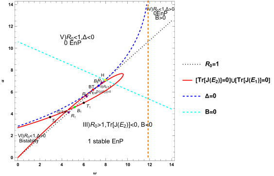
Figure 3: Same figure, with the curve $Tr\left(J_{E_{2}}\right)=0$ replaced by the easier to compute $\left[Tr\left(J_{E_{2}}\right)=0\right]\cup\left[Tr\left(J_{E_{1}}\right)=0\right]$

   which eliminates the variables $\{s,i\}$ from the Trace of the Jacobian. This allows producing a plot of both branches of the curve $\left[Tr\left(J_{E_{2}}\right)=0\right]\cup\left[Tr\left(J_{E_{1}}\right)=0\right]$, together ( see Figure 3) (and includes our desired curve ${Tr\left(J_{E_{2}}\right)=0}$). This approach is explained in more detail in Section 4.2.

   A similar alternative approach is to compute the functions $tr(i),p(i)$ which depend on $i$ but not on $s$, and their resultant. Both these approaches work very quickly, but do not allow separating the two branches. This may only be achieved via the numeric approach described next.

2. Explicitize $i=i_{2}$ and continue with numeric values for all parameters, except the two chosen to be displayed (using rational numbers, to be able to work with infinite precision) – see Figure 2.

We report on both approaches in next section, as well as in a “symbolic notebook” containing whatever could be computed symbolically: fixed points, bifurcation varieties, and their intersections. This produces the two dimensional map obtained by evaluating our curves under a “cut numeric condition” for the remaining parameters, and examines examples of points in most of the regions, and on their boundaries. Here we must clarify that a very important part of a numeric bifurcation project involving many parameters is to obtain an interesting cut where all the parameters but two are fixed. This may be achieved by packages for “numerical continuation and bifurcation” of ODE dynamical systems like MatCont (written in Matlab), PyDSTool (Python), XPPAuto (C), and BifurcationsKit (Julia) – see [BRM20] for a recent review. In our paper, we just perturbed a bit the cut furnished in [ZF12], until it became clearer that the coincidence of the four curves in their paper was an optical illusion.

Finally, we offer a second “numeric notebook” which uses the Mathematica contributed package EcoEvo, which helps to produce quickly the time and phase-plots illustrating the various points chosen for display.

4.2 A key tool: computing Bogdanov-Takens bifurcations using symbolic algebra

Symbolic stability and bifurcation analysis are very time consuming, since they require identifying varieties like traces, determinants and Hurwitz determinants, evaluated at all the fixed points. It is plausible however that the equation satisfied by the union over the fixed points (i.e. the product of all the respective equations), ends up simpler symbolically.

Before presenting the bifurcation results for our example, we present now some useful symbolic objects which we have introduced, and were not able to find in the previous dynamical systems literature.

Definition 1

The determinant, trace, and Hurwitz determinant of an algebraic system with respect to a subset of its solutions $A$ is defined by the expressions

$$\begin{cases}detE=\prod_{i\in{\mathcal{A}}}Det(J(E_{i}))\\ trE=\prod_{i\in{\mathcal{A}}}Tr(J(E_{i}))\\ H_{n,E}=\prod_{i\in A}H_{n}(E_{i}).\end{cases}$$ (4.5)

Remark 5

1. Two choices of ${\mathcal{A}}$ are of special interest: one, involving the product of the traces over all the fixed points, is useful for general dynamical systems. Another one, involving only the product over the interior points, is the one we used mostly, since eliminating the DFE from the study is advantageous computationally, and anyway the DFE is easy to study separately.

2. The varieties corresponding to $detE,trE$, etc, are the union of the varieties for each branch. Due to the Vieta relations between the roots, they are expected to be considerably simpler than the individual expressions for the various branches.

3. Interestingly, $detE,trE$, etc seem related up to proportionality to the results obtained via the GroebnerBasis elimination command

   $$\begin{cases}{detG}=\text{GroebnerBasis}[Numerator[Together[[\{\text{dyn}[[1]],\text{dyn}[[2]],Det(X)\}]],\text{par},X]\\ {trG}=\text{GroebnerBasis}[Numerator[Together[[\{\text{dyn}[[1]],\text{dyn}[[2]],Tr(X)\}]],\text{par},X]\end{cases},$$ (4.6)

   which are easily obtained via the script:

    GBH[mod_,scal_,cn_ : {}] :=
        GroebnerBasis[Numerator[Together[[Join[ mod[[1]], {scal}]]],
        mod[[3]],  mod[[2]]]
   

   (recall that mod={dyn,var,par}). To resolve a two dimensional model, it is enough to apply this script with scal= trace and scal=determinant.

4. The proportionality might be caused by spurious implementation factors. It may be interesting to clarify the relation between ${detE},{trE}$ and the corresponding Mathematica objects ${detG},{trG}$.

Remark 6

1. The computation of candidates for the Bogdanov-Takens bifurcations for all the fixed points in two dimensions may be achieved a priori via the single command
   

   $$Reduce[\{trG==0,detG==0,cp\}],$$ (4.7)

   where cp are positivity and other eventual constraints on the variables and parameters.

   For the [ZF12] model, we find in the third cell of [Ade22] that detG is proportional to the product of $R_{0}-1$ and the discriminant, and that trG is proportional to the product of

   $$\begin{cases}\omega-\frac{(\gamma+\delta+\mu)\left(2\mu(\gamma+\delta+\eta)+(\gamma+\delta)(\gamma+\delta+\eta)+\mu^{2}\right)}{(\gamma+\delta+\eta+\mu)\left(\beta\eta+\xi\left(2\mu(\gamma+\delta+\eta)+(\gamma+\delta)(\gamma+\delta+\eta)+\mu^{2}\right)\right)},\\ \xi\omega^{2}(\beta+\mu\xi)^{2}(\gamma+\delta+\eta+\mu)-\omega(\beta+\mu\xi)(\beta\eta+\mu\xi(2\gamma+2\delta+\eta+2\mu))+\mu^{2}\xi(\gamma+\delta+\mu)\end{cases}$$ (4.8)

   and a third order polynomial in $\omega$ which has one rational root.

   Since (4.7) takes too much time, we decompose into $4$ equalities corresponding to all combinations of the factors.

2. In more dimensions, it is enough a priori to replace the trace in (4.7) by the maximal dimension Hurwitz determinant, and investigate also the positivity conditions associated to the other Hurwitz determinants.

For the generalization of [ZF12], the detG can be obtained, but trG exceeds our computing time (more than one night). We turn therefore from now on to the particular case of [ZF12].

4.3 The corrected two parameter bifurcation diagram

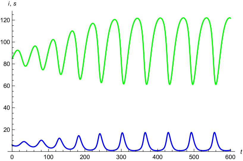
(a) $(s,i)$-time plot indicate the existence of a limit cycle surrounding $E_{2}$

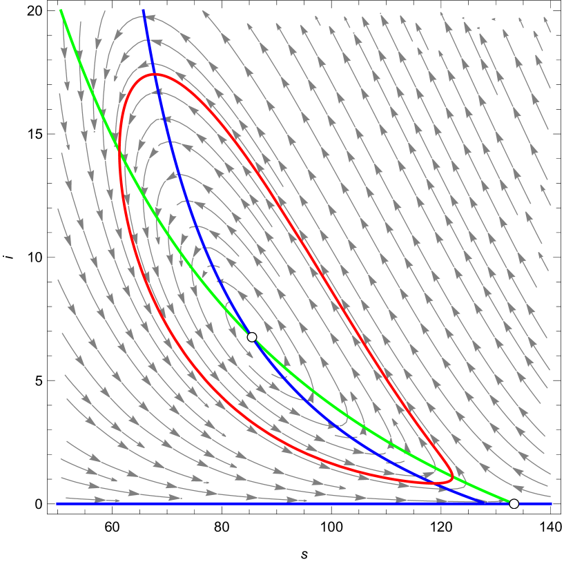
(b) $(\mathsf{s},\mathsf{i})$- phase plot. Attracting orbit with period $63.5036$, and Floquet exponents $\left(-1.2044\times 10^{-8},-0.0228667\right)$.

Figure 5: Time and phase-plot corresponding to region II in Figure 2,with $\left\{\omega=51/8,\alpha=43/8\right\}\Longrightarrow{\mathcal{R}}_{0}=1.03912>1$.

We correct here the two-parameter bifurcation diagram in [ZF12, Fig. 6]. Our model has $8$ parameters, or rather seven, since $\delta,\gamma$ intervene in the first two equations only via their sum. Recall that [ZF12, Fig. 5-6] offer values for six of the parameters ($b=16,\mu=\frac{1}{10},\delta=\frac{2}{10},\gamma=\frac{12}{100},(\Longrightarrow v_{i}=\frac{42}{100}),\beta=\frac{1}{100},\xi=\frac{1}{1000}$) which produced an interesting partition of the two parameter space of the remaining “treatment parameters” $(\omega,\eta)$. We have changed however one parameter to $\mu=.12$ – see Figure 2, and [Mat22b], since this makes evident that the point $e$ in [ZF12, Fig. 6], through which four curves seem to pass, is an optical illusion (which hides a region VII which is revealed after a further blow-up in Figure 4).

For comparison with the original, we will show our figure with $\eta$ replaced by the [ZF12] parameter $\alpha=\eta\omega$.

The parameter space is divided in 7 regions, defined by the signs of $\Delta,{\mathcal{R}}_{0}-1,Tr(J(E_{2}))$, called respectively I,II,III,IV,V,VI,VIa; the corresponding sign patterns, including that of ${B}$ (which turns out helpful) are given in the following table:

Table 1: Table of the sign patterns corresponding to the six regions.

	sign of $\Delta$	sign of ${\mathcal{R}}_{0}-1$	sign of $Tr(J(E_{2}))$	sign of B
Region I ($Q_{I}$)	$>0$	$<0$	$>0$	$<0$
Region II ($Q_{II}$)	$>0$	$>0$	$>0$	both
Region III ($Q_{III}$)	$>0$	$>0$	$<0$	both
Region IV ($Q_{IV}$)	$>0$	$<0$	$>0$	$>0$
Region V ($Q_{V}$)	$<0$	$<0$	$>0$	both
Region VI ($Q_{VI}$)	$>0$	$<0$	$<0$	$<0$
Region VI ($Q_{VIa}$)	$>0$	$<0$	$<0$	$<0$
H	=0	=0	$>0$	=0
BT	=0	$<0$	=0	$<0$
$B_{1},B_{2}$	$>0$	=0	=0	$<0$

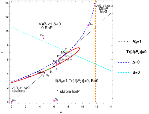
Figure 2: The partition of the $(w,\alpha)$ plane into seven regions, defined by ${\mathcal{R}}_{0}=1,\Delta=0,Tr\left(J_{E_{2}}\right)=0$ (which is involved in determining the Hopf bifurcation variety), and $B=0$ (the crossing of which changes the number of endemic points between the regions I,V from $2$ to $0$). Note that the region $Tr\left(J_{E_{2}}\right)<0$ is included in the region $\Delta\geq 0$, confirming the fact that this yields the stability region for $E_{2}$ [ZF12, Thm 3.3], [GK22, Thm. 3]. The trace curve $Tr\left(J_{E_{2}}\right)=0$ of possible Hopf points ends at the point $BT$, due to the fact that we broke here it’s twin part $Tr\left(J_{E_{1}}\right)=0$ –see Figure 3, where no Hopf bifurcations may appear. This curve may further be divided in an upper part separating regions II and III and a lower part separating regions I and VI. When crossing the upper part, the stability of the point $E_{2}$ and hence of the cycle surrounding it changes. When crossing the lower part from region III into region VI, it was conjectured but not proved in [ZF12, Fig.6] that periodic non-attracting orbits appear in a neighborhood of the boundary. We verify this numerically below in figures 6, 7 and 16.

Remark 7

The point H when both the endemic points collide with the DFE is at the intersection of the curves $\begin{cases}B=0\\ C=0\Leftrightarrow{\mathcal{R}}_{0}=1\end{cases}$, where $B,C$ are defined in (3.4). It is easy to determine: $\begin{cases}{\mathcal{R}}_{0}=1\Longrightarrow V_{i}=\frac{\Lambda}{\mu}\beta\\ B=0\Longrightarrow V_{i}=\frac{\mu\eta}{v_{1}\omega}\end{cases}$ yields

$$\begin{cases}\eta_{H}=\eta_{0}=\frac{\beta\Lambda}{\mu}-v_{i},\\ \omega_{H}=\frac{\mu^{2}\eta_{0}}{\beta\Lambda v_{1}}\Longrightarrow\alpha_{H}={\eta_{0}\omega_{H}=\frac{\mu^{2}\eta_{0}^{2}}{\beta\Lambda v_{1}}}\end{cases}$$ (4.9)

The fact that $Tr(E_{2})=0$ in Figure 1 of [ZF12] was an illusion; in fact, $Tr_{H}(E_{2})=-\mu$. However, $\Delta_{H}=0$, since

$$\Delta_{{\mathcal{R}}_{0}=1}=\frac{\left(\beta\Lambda\omega v_{1}-\mu^{2}(\beta\Lambda/\mu-v_{i})\right)^{2}}{\mu^{2}}=\frac{\beta\Lambda v_{1}}{\mu^{2}}\left(\omega-\omega_{H}\right)^{2}.$$

The points at the intersection of ${\mathcal{R}}_{0}=1$ with $tr(E_{2})=0$ may be determined symbolically, for example by computing the resultant of $p(i)$ and the numerator of $tr(i)$ under the condition $\eta=\eta_{0}$, and solving it with respect to  $\omega$.

Assuming $\widetilde{{\mathcal{R}}_{0}}\neq 1,\omega\neq\mu/v_{1}$, this yields that $\omega$ is one of the roots of a third order polynomial to be called “B-points”.

In the example illustrated in the figure 1 we find, besides the H point, three B points, and a “BT” (Bermuda triangle) point, at the intersection of the trace and discriminant curves.We exclude the third B point, since it belongs to the $Tr(E_{1})=0$ branch. The remaining points, together with other points along the boundary $\mathcal{R}_{0}=1$, ordered by $\omega$, are:

$$\begin{cases}R_{1}=\;\{\omega\to 4.620,\alpha\to 4.127\}\mbox{ (on ${\mathcal{R}}_{0}=1$, downward from $B_{1}$)}\\ B_{1}=\{\omega\to 5.157,\alpha\to 4.607\}\\ R_{2}=\{\omega\to 6.258,\alpha\to 5.590\}\mbox{(on ${\mathcal{R}}_{0}=1$, upward from $B_{1}$)}\;\\ BT=\{\omega\to 6.841,\alpha\to 6.203\}\\ R_{3}=\{\omega\to 7.652,\alpha\to 6.835\}\mbox{ (on ${\mathcal{R}}_{0}=1$, between $B_{2}$ and H)}\;\\ B_{2}=\{\omega\to 7.359,\alpha\to 6.574\}\\ H=\{\omega\to 7.944,\alpha\to 7.097\}\\ \end{cases}.$$

We also display the interior points

$$\begin{cases}Q_{I}=\{\omega\to 2.156,\alpha\to 3.468\}\\ Q_{II}=\{\omega\to 6.375,\alpha\to 5.375\}\\ Q_{III}=\{\omega\to 6,\alpha\to 0.156\}\\ Q_{IV}=\{\omega\to 11.75,\alpha\to 11.75\}\\ Q_{V}=\{\omega\to 6,\alpha\to 6\}\\ Q_{VI}=\{\omega\to 0.078,\alpha\to 0.156\}\end{cases}$$

and some points along the boundary $Tr(E_{2})=0$

$$\begin{cases}T_{1}=\{\omega\to 6,\alpha\to 5.00625\}\\ T_{2}=\{\omega\to 2.932,\alpha\to 3.696\}\end{cases}$$

Remark 8

Note the middle two points $BT$ and $B_{2}$ are hard to distinguish at any scale by eye, since in between them the $\Delta=0,$ its ${\mathcal{R}}_{0}=1$ tangent at $H$, and $Tr(E_{2})=0$ practically coincide. Together with the point $H$, these points give rise to a “Bermuda triangle, where the phase-plot looks like in Figure 4 below.

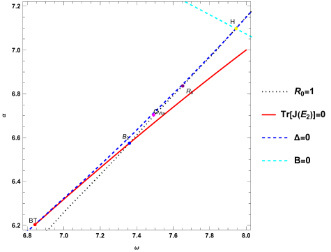
Figure 4: The Bermuda triangle

4.4 Some time and phase plot illustrations of the dynamics in the various regions

We undertake now a journey between the six regions in Figure 2, showing phase and time-plots for specific parameter values. We switch from now on to using the package EcoEvo in our electronic notebook [Mat22a], which has the advantage of computing also the period of cycles and their Floquet numbers.

We start in the region II, where the surprising absence of stable fixed points (this does not seem to occur in simple models without functional parameters) implies the existence of at least one stable limit cycle.

4.4.1 Region II, with all the fixed points unstable

A random choice of parameters confirms that at our first choice (obtained using FindInstance) there exists indeed at least one stable limit cycle, which surrounds the unique unstable spiral point $E_{2}=(85.4965,6.75961)$ with eigenvalues $0.00887972\pm 0.13495\;Im$. The DFE  $E_{0}=(133.333,0)$ is a saddle point with eigenvalues $(-0.12,0.0501961)$, and the point $E_{1}$ is outside the positive orthant.

In the next five sections we will investigate the spread of oscillations into the neighboring regions III and I, and at the corner points $B_{1},B_{2},BTP$.

4.4.2 Spread of oscillations into the neighboring region III

At the boundary between regions II and III it holds that $Tr(J(E_{2}))=0$; at $T_{1}=\left\{\omega=6,\alpha=5.00625\right\}$, $E_{2}$ is a potential Hopf point. Our first choice, obtained using FindInstance, suggests that the endemic point $E_{2}=(80.6403,7.90317)$ with eigenvalues $\pm 0.15125Im$ is surrounded by a stable limit cycle. The disease free equilibrium  $E_{0}=(133.333,0)$ is a saddle point with eigenvalues $(-0.12,0.0589583)$, and the fixed point $E_{1}$ is outside the positive orthant.

Crossing now inside region III, the endemic point $E_{2}$ becomes stable [ZF12, Thm 3.3],

The cycle is at first unstable ”near the boundary”, and then disppears “far enough” from the boundary. The interior point $E_{2}=(45.58,23.6495)$ is an attracting spiral with eigenvalues $-0.178557\pm 0.265984\;Im$. The disease free equilibrium  $E_{0}=(133.333,0)$ is a saddle point with eigenvalues $(0.867292,-0.12)$, and the fixed point $E_{1}$ is outside the domain.

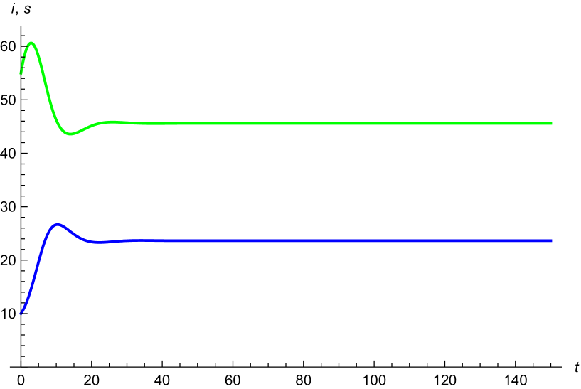
(a) $(s,i)$-time plot indicate the convergence towards the endemic point $E_{2}=(45.58,23.6495)$

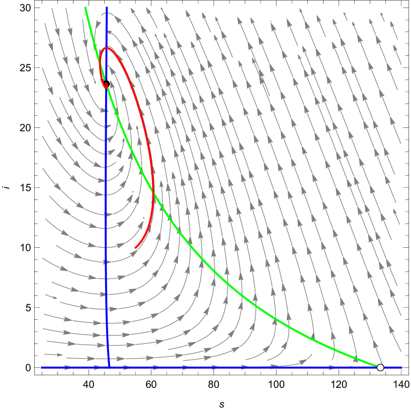
(b) $(\mathsf{s},\mathsf{i})$- phase plot.

Figure 7: Time and phase-plot corresponding to region III in Figure 2,with $\left\{\omega=6,\alpha=5/32\right\}$.

4.4.3 Spread of oscillations into the neighboring region I

Recall that in region II, the absence of any fixed stable points implies the existence of at least one stable limit cycle. This is still true on the boundary $\mathcal{R}_{0}=1$ with region I, from $B_{1}$ to $B_{2}$.

For example, at the point $\left\{\omega=7.16058,\alpha=6.39679\right\}$, the following figure reveals the existence of an unstable limit cycle around the endemic point $E_{2}=(111.34,2.376)$ with eigenvalues $0.0103906\pm 0.0502167\;Im$. The two fixed points $E_{0}=E_{1}=(133.333,0)$ collide with eigenvalues $(-0.12,0)$.

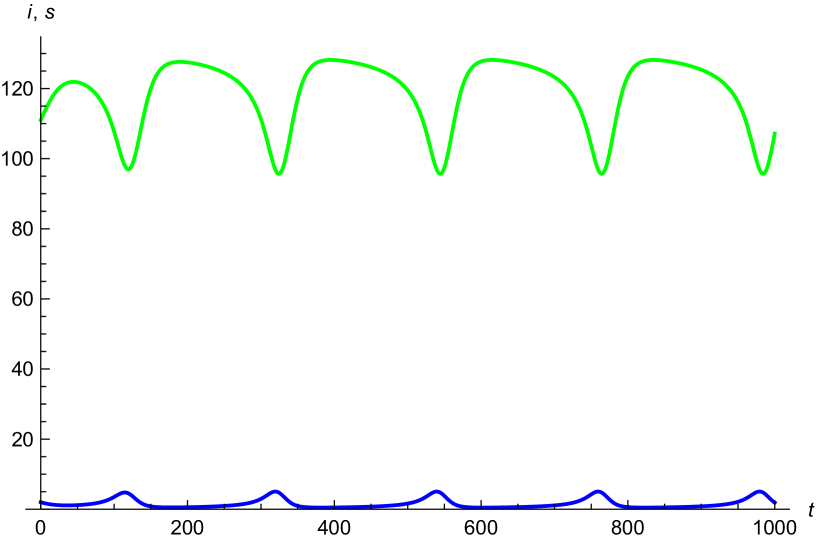
(a) $(s,i)$-time plot shows the existence of limit cycle surrounding $E_{2}$

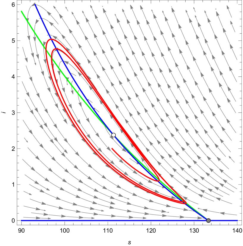
(b) $(\mathsf{s},\mathsf{i})$- phase plot. The period of the cycle is $219.938$ and the Floquet exponents are $\left\{-2.73386\times 10^{-8},-0.0298991\right\}$.

Figure 8: Time and phase-plot corresponding the neighboring region I at the point $\left\{\omega=7.16058,\alpha=6.39679\right\}$ in Figure 2.

By continuity, cycles must still exist within region I, close to the boundary. This is somewhat surprising, since the DFE is now stable.

4.4.4 Existence of Hopf-point at $B_{1}=\left\{\omega=5.15735,\alpha=4.60724\right\}$

This is the meeting point of regions I, II, III and VI. Here $\mathcal{R}_{0}=1\Longrightarrow$ $E_{0}=(133.333,0)=E_{1}$ is a saddle point with eigenvalues $(-\mu=-0.12,0)$, and the endemic point $E_{2}=(78.5251,8.44639)$ is a Hopf-point with eigenvalues $\pm 0.152171\;Im$, and $Tr[J(E_{2})]=0$. An unstable limit cycle around $E_{2}$ arises.

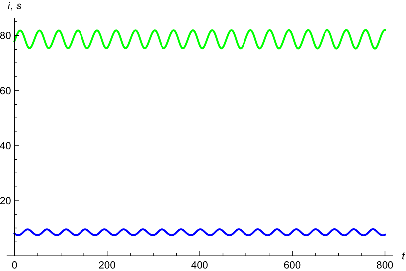
(a) $(s,i)$-time plot indicate the existence of a limit cycle surrounding $E_{2}$

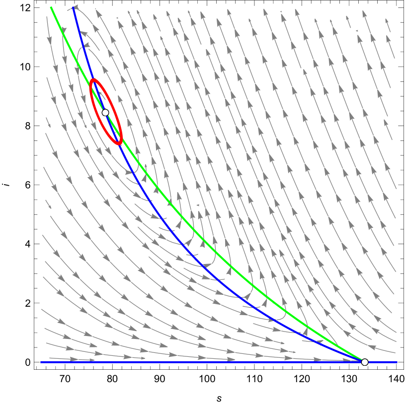
(b) $(\mathsf{s},\mathsf{i})$- phase plot. The cycle has period $42.2252$, and Floquet exponents $\left\{0.00181877,-0.000205883\right\}$

Figure 9: Time and phase-plot corresponding to the boundaries $\mathcal{R}_{0}=1,Tr[J(E_{2})]=0$ at the point $B_{1}=\left\{\omega=5.15735,\alpha=4.60724\right\}$ in Figure 2.

4.4.5 The point $B_{2}$ where regions II, III,VI,VIa meet

At $B_{2}=(7.35966,6.57463)$, one of the two solutions of $\mathcal{R}_{0}=1,Tr(E_{2})=0$, a stable limit cycle arises around the Hopf-point $E_{2}=(116.198,1.77275)$ with eigenvalues $\pm 0.0391099\;Im$, while the other unstable fixed points $E_{0}=(133.333,0)=E_{1}$ collide with eigenvalues $(-0.12,0)$.

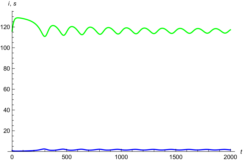
(a) $(s,i)$-time plot shows the existence of limit cycle surrounding $E_{2}$

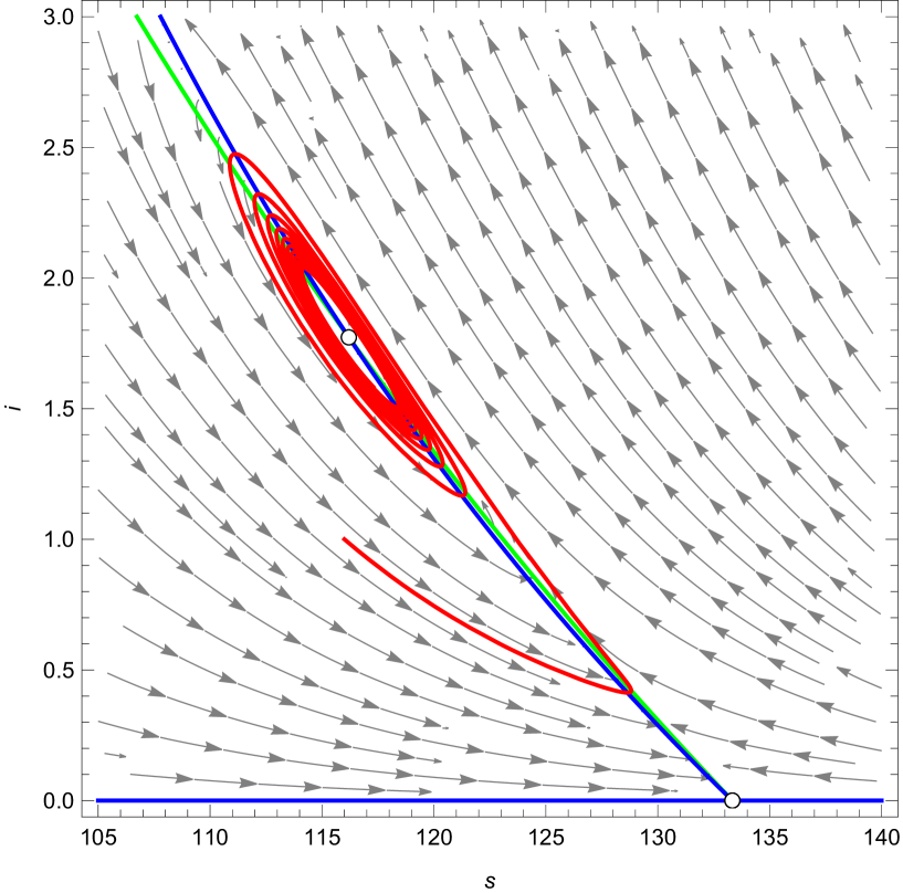
(b) $(\mathsf{s},\mathsf{i})$- phase plot. The cycle has period $160.805$ and the Floquet exponents are $\left\{-0.0000365264,-0.000058307\right\}$.

Figure 10: Time and phase-plot corresponding at the point $B_{2}=(7.35966,6.57463)$ in Figure 2.

4.4.6 Phase-plot illustration at the point $BT$ where regions III,V,VI,VIa meet

Now moving to the point $BT=(\omega=6.84183,\alpha=6.20319)$ , the following figures indicate the convergence towards the disease free equilibrium  $E_{0}=(133.333,0)$ which is stable with eigenvalues $(-0.12,-0.0133232)$, and the remaining fixed points $E_{1}=E_{2}=(117.951,1.56737)$ exhibits the existence of a Bogdanov-Takens bifurcation since the eigenvalues are $\left(0,0\right)$.

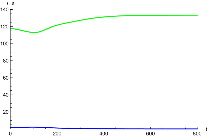
(a) $(s,i)$-time plot reveals convergence towards the disease free equilibrium

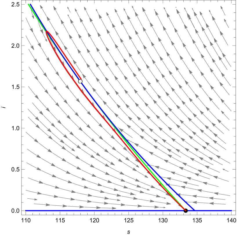
(b) $(\mathsf{s},\mathsf{i})$- phase plot.

Figure 11: Time and phase-plot at the point $BT=(6.84183,6.20319)$ in Figure 2.

4.4.7 The point $H$ at the intersection of $\mathcal{R}_{0}=1$ and $\Delta=0$

At $H=\left\{\omega=7.94466,\alpha=7.09723\right\}$, the solution of $\mathcal{R}_{0}=1$ and $\Delta=0$, the three fixed points coalesce as the figure below illustrates.

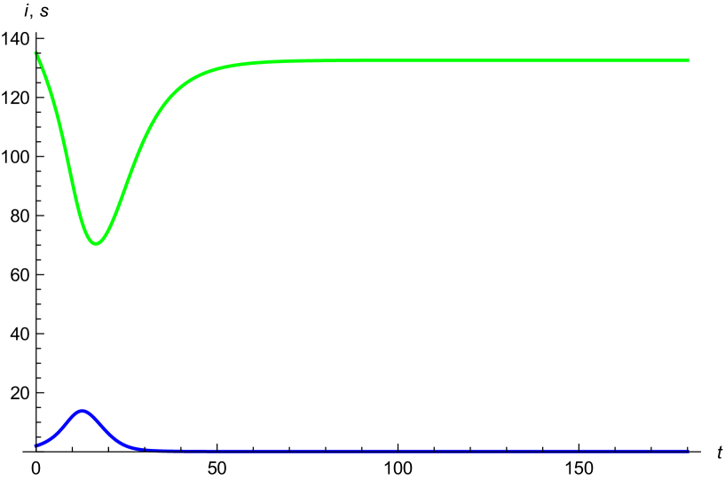
(a) $(s,i)$-time plot reveals convergence towards the disease free equilibrium

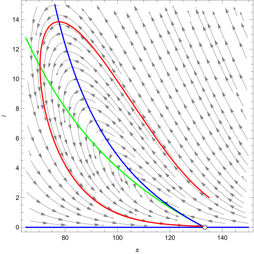
(b) $(\mathsf{s},\mathsf{i})$- phase plot. The fixed points $E_{0}=E_{1}=E_{2}=(133.333,0)$ collide with eigenvalues $(-0.12,0)$.

Figure 12: Time and phase-plot corresponding to the boundary $\mathcal{R}_{0}=1$ at the point $H$ in Figure 2, with $\left\{\omega=7.94466,\alpha=7.09723\right\}\Longrightarrow\mathcal{R}_{0}=1$.

4.4.8 Dynamical behaviour at region VIa

Now moving inside the region VIa where we have bistability of $E_{2}=(122.3268072,1.080883)$ the disease free equilibrium $E_{0}=(133.333,0)$ with eigenvalues respectively, $-0.01676672\pm 0.01328093\;Im$ and $(-0.12,-0.0014)$. The point $E_{1}=(130.4528,0.265)$ is a saddle point with eigenvalues $(-0.09477,0.0013)$.

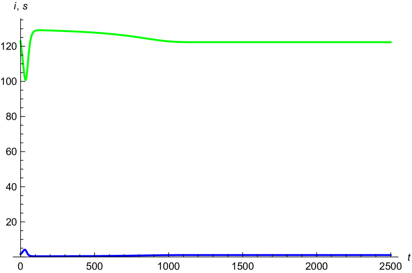
(a) $(s,i)$-time plot indicate the convergence towards $E_{2}$

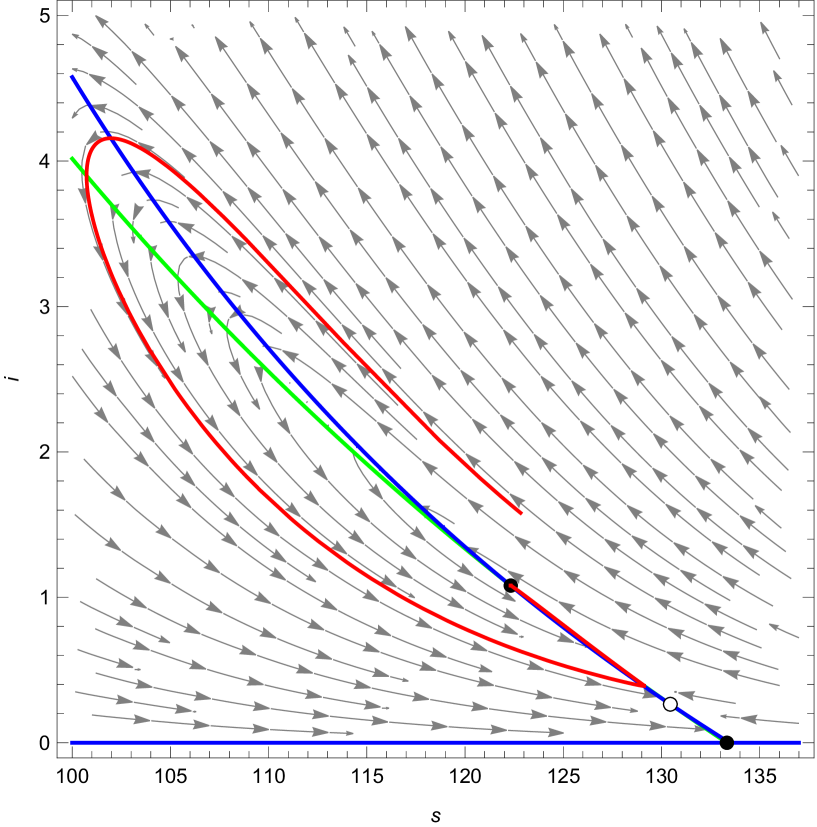
(b) $(\mathsf{s},\mathsf{i})$- phase plot. The stable attractor $E_{2}$ is surrounded by the red trajectory.

Figure 13: Time and phase-plot corresponding to region VIa in Figure 2,with $\left\{\omega=502/67,\alpha=41102/6131\right\}$.

4.4.9 The boundary $Tr(E_{2})=0$ between regions VIa and I

At $T_{2}=\left\{\omega=2.93233,\alpha=3.69658\right\}$, the stability of the DFE remains, and the endemic point The fixed point $E_{2}=(73.82,9.770)$ becomes a Hopf point with eigenvalues $\pm 0.152\;Im$ and it’s surrounded by an unstable limit cycle. The DFE  $E_{0}=(133.333,0)$ is stable with eigenvalues $(-0.367,-0.12)$, and the point $E_{1}=(106.9,2.971)$ is a saddle point with eigenvalues $(0.229,-0.0664)$.

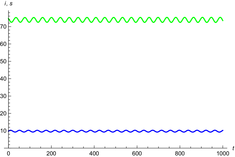
(a) $(s,i)$-time plot indicate the existence of a limit cycle surrounding $E_{2}$

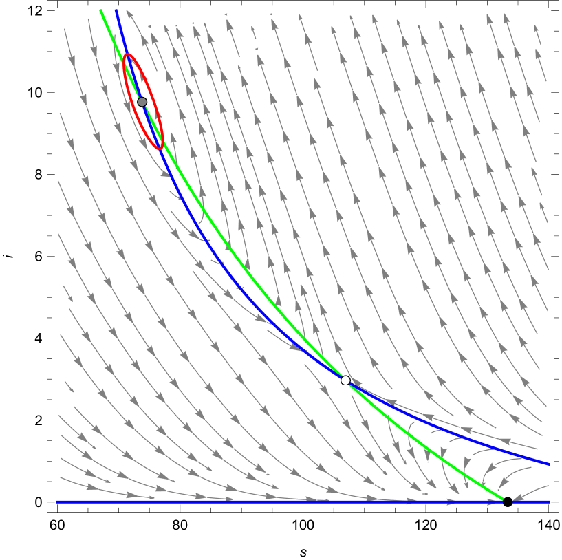
(b) $(\mathsf{s},\mathsf{i})$- phase plot. The cycle has period $41.7589$ and Floquet exponents $\left\{0.00149016,0.000030097\right\}$.

Figure 14: Time and phase-plot corresponding to boundary $Tr(E_{2})=0$ between regions VIa and I in Figure 2,with $\left\{\omega=2.93233,\alpha=3.69658\right\}$.

4.4.10 The boundary $\mathcal{R}_{0}=1$ between $B_{2}$ and $H$

Moving on the boundary $\mathcal{R}_{0}=1$ towards the point $H=(7.94466,7.09723)$ with $\omega=7.91732,\;\alpha=7.0728$. The endemic point $E_{2}=(132.419,0.0828753)$ is a stable with eigenvalues $(-0.111746,-0.0000342071)$. The disease free equilibrium $E_{0}=(133.333,0)=E_{1}$ is a saddle point with eigenvalues $(-0.12,0)$. The following figures show the convergence towards the disease free equilibrium.

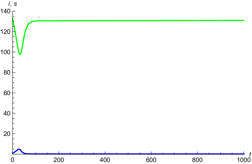
(a) $(s,i)$-time plot shows the convergence towards the disease free equilibrium

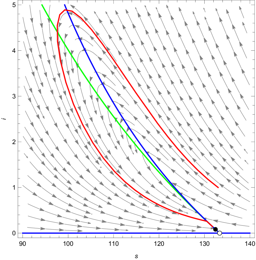
(b) $(\mathsf{s},\mathsf{i})$- phase plot.

Figure 15: Time and phase-plot corresponding to boundary $\mathcal{R}_{0}=1$ between $B_{2}$ and $H$ with $\omega=7.91732,\;\alpha=7.0728$ in Figure 2.

4.4.11 The boundary $\mathcal{R}_{0}=1$ between regions III and VI

At the point $R_{1}=\left(\omega=4.62051,\alpha=4.12766\right)$, and moving downwards from $B_{1}=(5.15735,4.60724)$, the following figures show the convergence towards the endemic point $E_{2}=(72.8175,10.0732)$ which is a stable attractor with eigenvalues $-0.017169\pm 0.173632\;Im$. The fixed points $E_{0}=E_{1}=(133.333,0)$ collide into a saddle with eigenvalues $(-0.12,0)$.

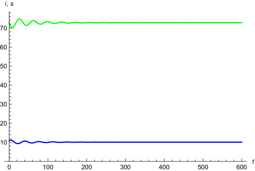
(a) $(s,i)$-time plot indicate the convergence towards $E_{2}$

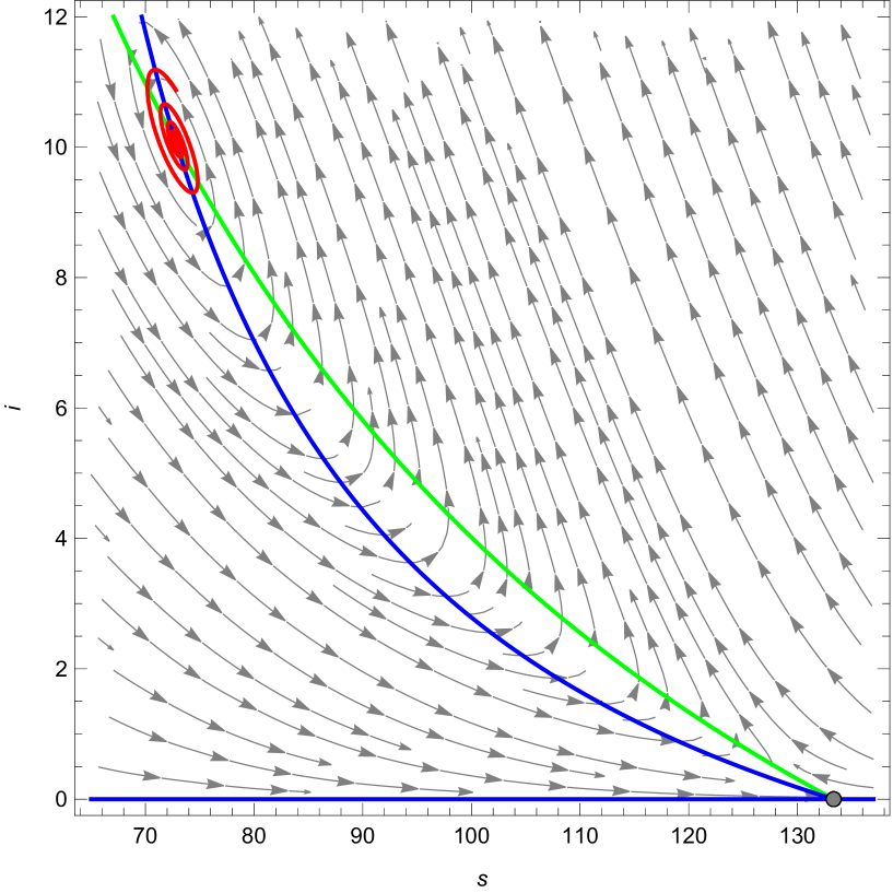
(b) $(\mathsf{s},\mathsf{i})$- phase plot.

Figure 16: Time and phase-plot corresponding to boundary $\mathcal{R}_{0}=1$ between regions III and VI at the point $R_{1}=\left(\omega=4.62051,\alpha=4.12766\right)$ in Figure 2.

Starting to move upwards on the boundary closer to the “B point” $B_{1}$ where regions $I,II,III,VI$ meet reveals in next Figure 18 a stable limit cycle, surrounding the unique unstable interior point $E_{2}=(79.9285,8.0827)$ with eigenvalues $0.00347509\pm 0.146926\;Im$, which is “almost homoclinic with respect to   $E_{0}=E_{1}=(133.333,0)$” (with eigenvalues $(-0.12,0)$).

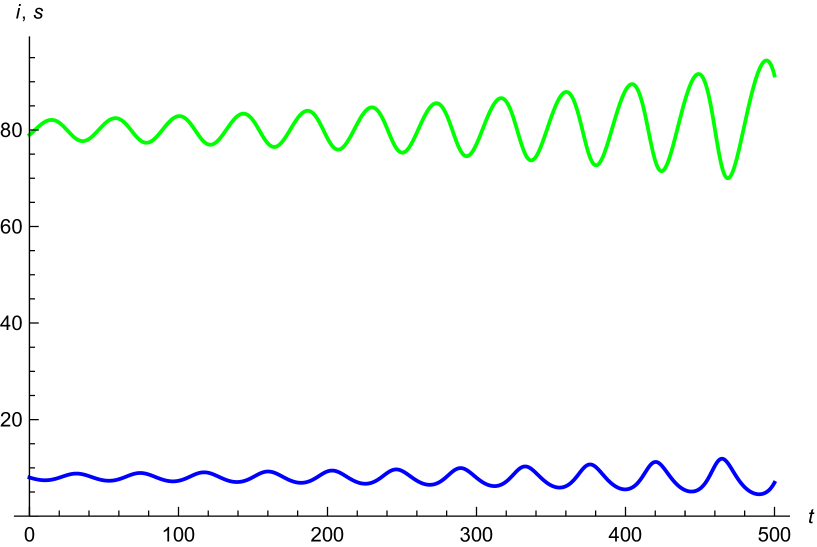
(a) $(s,i)$-time plot indicate the existence of a limit cycle surrounding $E_{2}$

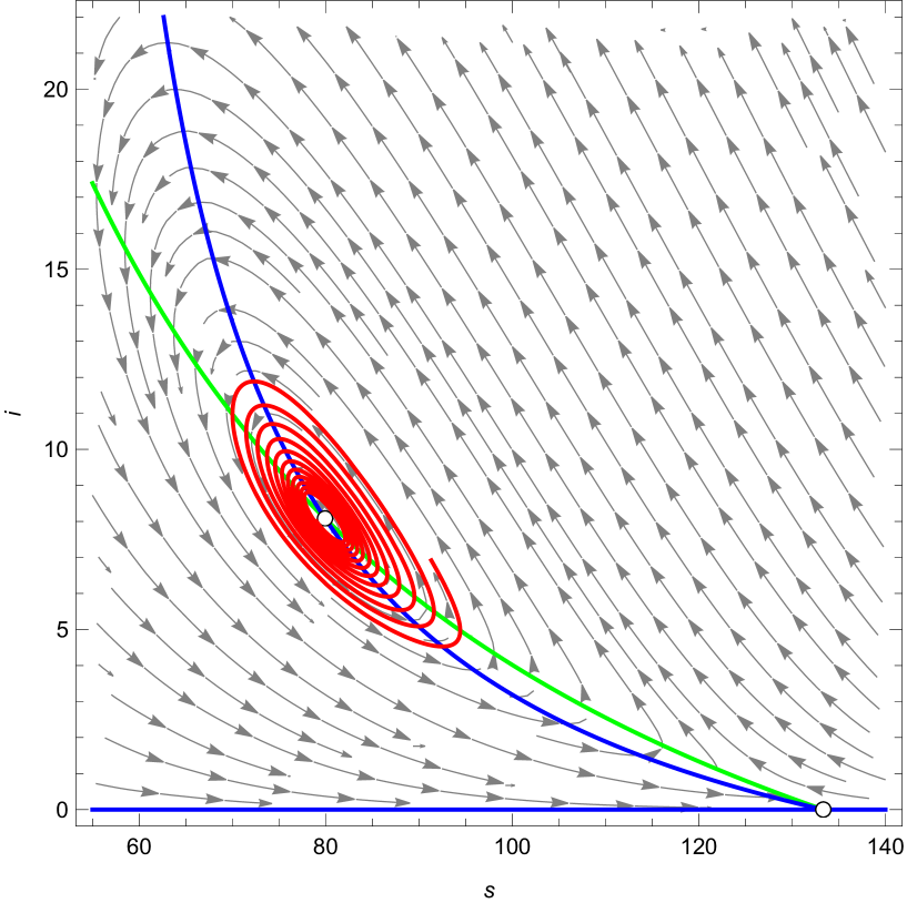
(b) $(\mathsf{s},\mathsf{i})$- phase plot. The period is $40.1628$, and the Floquet exponents $-0.00353727\pm 0.000583175\;Im$

Figure 17: Time and phase-plot corresponding to boundary $\mathcal{R}_{0}=1$ between regions I and II in Figure 2, with $\left\{\omega=723/137,\alpha=16147/3425\right\}\Longrightarrow\mathcal{R}_{0}=1$.

We continue now moving further upwards from $B_{1}=\left\{\omega=4.60724,\alpha=5.15735\right\}$ and getting closer to $BT=(6.84183,6.20319)$, on the boundary $\mathcal{R}_{0}=1$ between regions II and I with $\left\{\omega=25/4,\alpha=67/12\right\}$. Since $\mathcal{R}_{0}=1$, the DFE equals $E_{1}=(133.333,0)$ with eigenvalues $(0,-0.12)$ , and the following figure reveals an unstable, “almost homoclinic” limit cycle, surrounding the endemic point $E_{2}=(93.5174,5.13535)$ with eigenvalues $0.0226741\pm 0.0987278\;Im$.

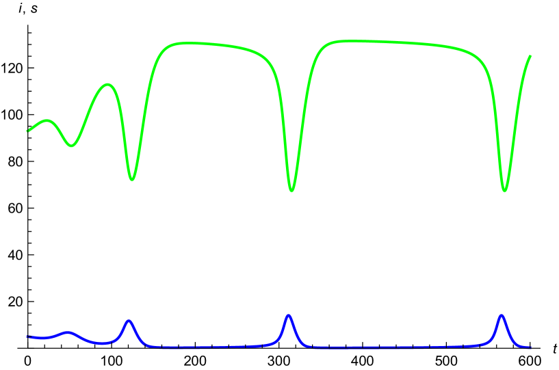
(a) $(s,i)$-time plot indicate the existence of a limit cycle surrounding $E_{2}$

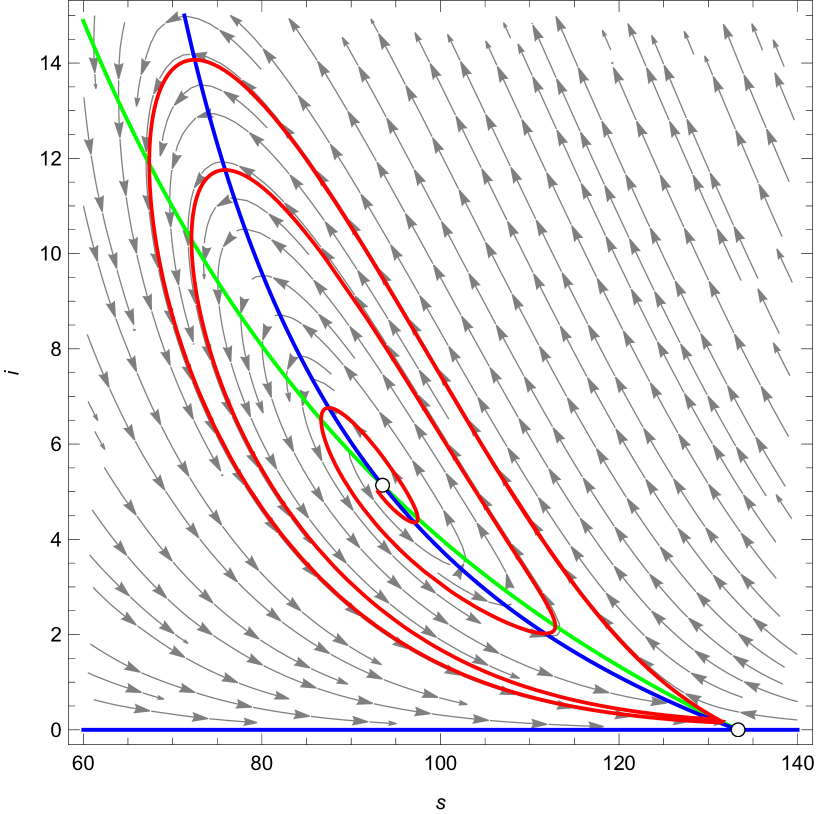
(b) $(\mathsf{s},\mathsf{i})$- phase plot. The period is $254.473$, and the Floquet exponents $\left\{-4.59451\times 10^{-8},-0.0659782\right\}$

Figure 18: Time and phase-plot corresponding to boundary $\mathcal{R}_{0}=1$ between regions I and II in Figure 2.

4.4.12 The bistability region VI (with DFE and $E_{2}$ stable and $E_{1}$ saddle)

In this region, at the point $Q_{VI}=\left(\omega=0.078125,\alpha=0.15625\right)$, both $E_{2}=(45.712,23.542)$ and the DFE $E_{0}=(133.33,0)$ are locally stable with eigenvalues $\left(-0.176845\pm 0.265287\;Im\right)$ and $(-1.1,-0.12)$, respectively. The fixed point $E_{1}=(132.24,0.098)$ is a saddle point with the corresponding eigenvalues $(0.4908,-0.1188)$. We illustrate in the following figures the convegence towards this two points and the corresponding phase-plot.

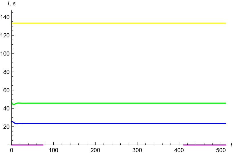
(a) $(\mathsf{s},\mathsf{i})-$time plots of indicate convergence towards $E_{2}$ and DFE.

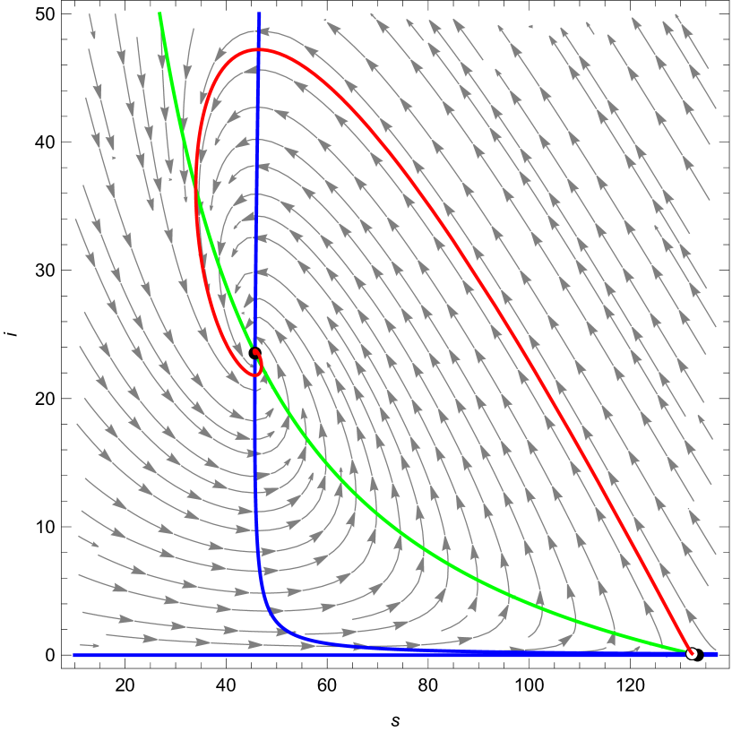
(b) $(\mathsf{s},\mathsf{i})$- phase plot.

Figure 19: Time and phase-plot corresponding to region VI at $Q_{VI}=\left(\omega=0.078125,\alpha=0.15625\right)$ in figure 2.

We have not found the claimed homoclinic cycle in [GK22, Fig. 1c)]

The problem of whether oscillations are possible in region VI away from the $B_{1}$ point is still open.

We skip the region I, where the DFE is the only stable point.

5 Appendix: A description of the accompanying Mathematica notebook

Writing a notebook for studying symbolically and numerically a dynamical system with seven parameters is a highly non-trivial task. This may be the explanation why a very small percentage of the literature is accompanied by notebooks.

We choose to organise our notebook [Mat22b] as follows:

• First cell enumerates the parameters to be studied.

• If we may want to use other parameters at a later time, in a future extension, we provide a condition setting them equal to $0$. We include here also notable particular cases.

• Afterwards, we provide definitions of simple fundamental quantities, which may be easily computed without Mathematica, and are “correct beyond any doubt”. In our case, we define the basic reproduction number  $\mathcal{R}_{0}$, and some critical parameters which make it equal to $1$ ($\beta,\eta$). In this way, we can specify the fundamental hypersurface $\mathcal{R}_{0}=1$ by fixing either $\beta$ or $\eta$.

• We provide then the essential conditions on the parameters (positivity).

• There will be also fundamental quantities which require a long time for computing and simplifying symbolically; these have been saved in the “package” ”def.m” and are loaded next.

  In our cases, they are the trace at the second endemic point, which is long that it requires 2 pages to display, and the discriminant $\Delta$. This equation reveals that the discriminant is only defined for $\omega v_{1}<\mu$, and that the curve $\Delta=0$ may be explicitized with respect to $\alpha$, which is clearly useful.

• We continue with some numerical conditions used in first tests, and with some conditions for switching between the parameters, for displaying alternative representations of the answers.

• The second cell contains the definition of the model, and fundamental quantities (fixed points, Jacobians, etc). Here we can either produce our own code, or use EcoEvo. We will provide both versions, since each has its advantages.

Declarations

Conflict of Interest: The authors have no competing interests to declare that are relevant to the content of this article.

References

- [AAB+21] Florin Avram, Rim Adenane, Lasko Basnarkov, Gianluca Bianchin, Dan Goreac, and Andrei Halanay, On matrix-sir arino models with linear birth rate, loss of immunity, disease and vaccination fatalities, and their approximations, arXiv preprint arXiv:2112.03436 (2021).
- [AABH22] Florin Avram, Rim Adenane, Gianluca Bianchin, and Andrei Halanay, Stability analysis of an eight parameter sir-type model including loss of immunity, and disease and vaccination fatalities, Mathematics 10 (2022), no. 3.
- [AAH22] Florin Avram, Rim Adenane, and Andrei Halanay, New results and open questions for sir-ph epidemic models with linear birth rate, loss of immunity, vaccination, and disease and vaccination fatalities, Symmetry 14 (2022), no. 5, 995.
- [Ade22] Rim Adenane, GitHub repository. Dynamics-of-a-sir-epidemic-model-with-limited-medical-resources https://github.com/Rim-Adenane/Dynamics-of-a-SIR-epidemic-model-with-limited-medical-resources, 2022.
- [BD95] Jonathan B Buckheit and David L Donoho, Wavelab and reproducible research, Wavelets and statistics, Springer, 1995, pp. 55–81.
- [BRM20] Mark Blyth, Ludovic Renson, and Lucia Marucci, Tutorial of numerical continuation and bifurcation theory for systems and synthetic biology, arXiv preprint arXiv:2008.05226 (2020).
- [CK92] Jon F Claerbout and Martin Karrenbach, Electronic documents give reproducible research a new meaning, SEG technical program expanded abstracts 1992, Society of Exploration Geophysicists, 1992, pp. 601–604.
- [CS78] Vincenzo Capasso and Gabriella Serio, A generalization of the kermack-mckendrick deterministic epidemic model, Mathematical biosciences 42 (1978), no. 1-2, 43–61.
- [Don10] David L Donoho, An invitation to reproducible computational research, Biostatistics 11 (2010), no. 3, 385–388.
- [FR00] Lorenzo Farina and Sergio Rinaldi, Positive linear systems: theory and applications, vol. 50, John Wiley & Sons, 2000.
- [GK22] RP Gupta and Arun Kumar, Endemic bubble and multiple cusps generated by saturated treatment of an sir model through hopf and bogdanov–takens bifurcations, Mathematics and Computers in Simulation (2022).
- [HCH10] Wassim M Haddad, VijaySekhar Chellaboina, and Qing Hui, Nonnegative and compartmental dynamical systems, Nonnegative and Compartmental Dynamical Systems, Princeton University Press, 2010.
- [HMR12] Zhixing Hu, Wanbiao Ma, and Shigui Ruan, Analysis of sir epidemic models with nonlinear incidence rate and treatment, Mathematical biosciences 238 (2012), no. 1, 12–20.
- [HVdD91] Herbert W Hethcote and P Van den Driessche, Some epidemiological models with nonlinear incidence, Journal of Mathematical Biology 29 (1991), no. 3, 271–287.
- [JNK16] Soovoojeet Jana, Swapan Kumar Nandi, and TK Kar, Complex dynamics of an sir epidemic model with saturated incidence rate and treatment, Acta biotheoretica 64 (2016), no. 1, 65–84.
- [Kla21] Chris Klausmeier, GitHub repository. EcoEvo . https://github.com/cklausme/EcoEvo, 2021.
- [LHL87] Wei-min Liu, Herbert W Hethcote, and Simon A Levin, Dynamical behavior of epidemiological models with nonlinear incidence rates, Journal of mathematical biology 25 (1987), no. 4, 359–380.
- [LHRY21] Min Lu, Jicai Huang, Shigui Ruan, and Pei Yu, Global dynamics of a susceptible-infectious-recovered epidemic model with a generalized nonmonotone incidence rate, Journal of dynamics and differential equations 33 (2021), no. 4, 1625–1661.
- [LL14] Guihua Li and Gaofeng Li, Bifurcation analysis of an sir epidemic model with the contact transmission function, Abstract and Applied Analysis, vol. 2014, Hindawi, 2014.
- [LLI86] Wei-min Liu, Simon A Levin, and Yoh Iwasa, Influence of nonlinear incidence rates upon the behavior of sirs epidemiological models, Journal of mathematical biology 23 (1986), no. 2, 187–204.
- [Mat22a] Mathematica, GitHub repository. Dynamics-of-a-sir-epidemic-model-with-limited-medical-resources https://github.com/Rim-Adenane/Dynamics-of-a-SIR-epidemic-model-with-limited-medical-resources/blob/main/EcoEvo-Vys2.nb, 2022.
- [Mat22b] , GitHub repository. Dynamics-of-a-sir-epidemic-model-with-limited-medical-resources https://github.com/Rim-Adenane/Dynamics-of-a-SIR-epidemic-model-with-limited-medical-resources/blob/main/ZF-Rev-F.nb, 2022.
- [MY20] Matthew Macauley and Nora Youngs, The case for algebraic biology: from research to education, Bulletin of Mathematical Biology 82 (2020), no. 9, 1–16.
- [PAVGA19] Angel GC Pérez, Eric Avila-Vales, and Gerardo Emilio Garcia-Almeida, Bifurcation analysis of an sir model with logistic growth, nonlinear incidence, and saturated treatment, Complexity 2019 (2019).
- [PHH21] Qin Pan, Jicai Huang, and Qihua Huang, Global dynamics and bifurcations in a sirs epidemic model with a nonmonotone incidence rate and a piecewise-smooth treatment rate, Discrete & Continuous Dynamical Systems-B (2021).
- [PS05] Lior Pachter and Bernd Sturmfels, Algebraic statistics for computational biology, vol. 13, Cambridge university press, 2005.
- [REAVGA16] Erika Rivero-Esquivel, Eric Avila-Vales, and Gerardo Garcia-Almeida, Stability and bifurcation analysis of a sir model with saturated incidence rate and saturated treatment, Mathematics and Computers in Simulation 121 (2016), 109–132.
- [RW03] Shigui Ruan and Wendi Wang, Dynamical behavior of an epidemic model with a nonlinear incidence rate, Journal of differential equations 188 (2003), no. 1, 135–163.
- [SW18] Gunog Seo and Gail SK Wolkowicz, Sensitivity of the dynamics of the general rosenzweig–macarthur model to the mathematical form of the functional response: a bifurcation theory approach, Journal of mathematical biology 76 (2018), no. 7, 1873–1906.
- [THRZ08] Yilei Tang, Deqing Huang, Shigui Ruan, and Weinian Zhang, Coexistence of limit cycles and homoclinic loops in a sirs model with a nonlinear incidence rate, SIAM Journal on Applied Mathematics 69 (2008), no. 2, 621–639.
- [VG16] Martin Vyska and Christopher Gilligan, Complex dynamical behaviour in an epidemic model with control, Bulletin of mathematical biology 78 (2016), no. 11, 2212–2227.
- [Wan06] Wendi Wang, Backward bifurcation of an epidemic model with treatment, Mathematical biosciences 201 (2006), no. 1-2, 58–71.
- [WR04] Wendi Wang and Shigui Ruan, Bifurcations in an epidemic model with constant removal rate of the infectives, Journal of Mathematical Analysis and Applications 291 (2004), no. 2, 775–793.
- [WXSL21] Wei Wei, Wei Xu, Yi Song, and Jiankang Liu, Bifurcation and basin stability of an sir epidemic model with limited medical resources and switching noise, Chaos, Solitons & Fractals 152 (2021), 111423.
- [XWJZ21] Yancong Xu, Lijun Wei, Xiaoyu Jiang, and Zirui Zhu, Complex dynamics of a sirs epidemic model with the influence of hospital bed number, Discrete & Continuous Dynamical Systems-B 26 (2021), no. 12, 6229.
- [ZF12] Linhua Zhou and Meng Fan, Dynamics of an sir epidemic model with limited medical resources revisited, Nonlinear Analysis: Real World Applications 13 (2012), no. 1, 312–324.
- [ZL08] Xu Zhang and Xianning Liu, Backward bifurcation of an epidemic model with saturated treatment function, Journal of mathematical analysis and applications 348 (2008), no. 1, 433–443.