Adaptive operator learning for infinite-dimensional Bayesian inverse problems

Abstract

The fundamental computational issues in Bayesian inverse problems (BIPs) governed by partial differential equations (PDEs) stem from the requirement of repeated forward model evaluations. A popular strategy to reduce such cost is to replace expensive model simulations by computationally efficient approximations using operator learning, motivated by recent progresses in deep learning. However, using the approximated model directly may introduce a modeling error, exacerbating the already ill-posedness of inverse problems. Thus, balancing between accuracy and efficiency is essential for the effective implementation of such approaches. To this end, we develop an adaptive operator learning framework that can reduce modeling error gradually by forcing the surrogate to be accurate in local areas. This is accomplished by fine-tuning the pre-trained approximate model during the inversion process with adaptive points selected by a greedy algorithm, which requires only a few forward model evaluations. To validate our approach, we adopt DeepOnet to construct the surrogate and use unscented Kalman inversion (UKI) to approximate the solution of BIPs, respectively. Furthermore, we present rigorous convergence guarantee in the linear case using the framework of UKI. We test the approach on several benchmarks, including the Darcy flow, the heat source inversion problem, and the reaction diffusion problems. Numerical results demonstrate that our method can significantly reduce computational costs while maintaining inversion accuracy.

1 Introduction

Many realistic phenomenons are governed by partial differential equations (PDEs), where the states of the system are described by PDEs solutions. The properties of these systems are characterized by the model parameters, such as the permeability and thermal conductivity, which can not be directly determined. Instead, the parameters can be inferred from the discrete and noisy observations of the states, which are known as inverse problems. Due to the fact that inverse problems are ill-posed in general, many methods for solving them are based primarily on either regularization theory or Bayesian inference. By imposing a prior distribution on the parameters, the Bayesian approach can provide a more flexible framework. The solutions to the Bayesian inverse problems, or the posterior distributions, can then be obtained by conditioning the observations using the Baye’s formula. In some cases, the model parameters are required to be functions, leading to infinite-dimensional Bayesian inverse problems. These cases possibly occur when the model parameters are spatially varying with uncertain spatial structures, which can be found in many realistic applications, including many areas of engineering, sciences and medicine [1, 2, 3, 4, 5].

The formulation of infinite-dimensional Bayesian inverse problems presents a number of challenges, including the well-posedness guaranteed by the proper prior selection, as well as the convergence of the solutions governed by the discretization scheme. Following that, dealing with the discrete finite-dimensional posterior distributions can be difficult due to the expensive-to-solve forward models and high-dimensional parameter spaces. As a result, direct sampling methods such as MCMC-based methods [6, 7, 8] will suffer from the unaffordable computation costs. Common methods to deal with these issues include (i) model reduction methods [9, 1, 10, 11], which exploit the intrinsic low dimensionality, (ii) direct posterior approximation methods, such as Laplace approximation and variational inference [12, 4], and (iii) surrogate modeling [13, 14, 15], which replaces the expensive model with a cheap substitute.

Surrogate modeling emerges as the most promising approach for efficiently accelerating the sampling of posterior distributions among the methods listed above. Deep learning methods, specifically deep neural networks (DNN), have recently become the most popular surrogate models in engineering and science due to their power in approximating high-dimensional problems[16, 17, 18, 19, 20]. In general, DNN employs the power of machine learning to construct a quick-to-evaluate surrogate model to approximate the parameter-to-observation maps[21, 15, 22]. Numerical experiments, such as those described in [15], demonstrated that with sufficiently large training datasets, highly accurate approximations can be trained. Traditional deep learning methods, on the other hand, frequently necessitate a large number of training points that are not always available. Furthermore, whenever the measurement operator changes, the surrogate should be retrained. Physical-informed neural networks(PINNs)[17] can address this issue by incorporating the physical laws into the loss function and learning the parameter-to-state maps[23, 24]. Due to this, they can be applied as surrogates for a class of various Bayesian inverse problems with models that are governed by the same PDEs but have various types of observations and noise modes, further reducing the cost of surrogate construction. However, PINNs have some limitations[25, 26], such as hyperparameter sensitivity and the potential for training instability due to the hybrid nature of their loss function. Several solutions have been proposed to address these issues[27, 28, 29, 30]. Furthermore, due to the requirement of a large collocation dataset, PINNs will continue to be ineffective for infinite-dimensional Bayesian inverse problems[23]. Operator neural networks, such as FNO[31] and DeepOnet[32], are able to model complex systems in high dimensional spaces as infinite-dimensional approximations. They are therefore promising surrogates, as described in[33, 34]. However, using approximate models directly may introduce a discrepancy or modeling error, exacerbating an already ill-posed problem and leading to a worse solution.

We propose in this paper to develop a framework that can adaptively reduce model error by forcing the approximate model to be locally accurate for posterior characterization during the inversion process. This is achieved by first using neural network representations of parameter-to-state maps between function spaces, and then retraining this initial model with points chosen adaptively using a greedy algorithm. The inversion process can continue using the fine-tuned approximate model with lower local model error. This procedure can be repeated multiple times as necessary until the stop criteria is met. For the detailed implementation, we use the DeepOnet[32] to approximate the parameter-to-state maps and the unscented Kalman inversion [35] to estimate the posterior distribution. Moreover, we can show that under the linear case, the convergence can be obtained if the surrogate is accurate throughout the space, which can also be extended to non-linear cases with locally accurate approximate models. To verify the effectiveness of our method, we propose testing several benchmarks including the Darcy flow, the heat source inversion problem and a reaction diffusion problem. Our main contributions can be summarized as the following points.

• We propose a framework for adaptively reducing the surrogate’s model error. To maintain local accuracy, the greedy algorithm is proposed for selecting adaptive samples for fine-tuning the pre-trained model.

• We adopt DeepOnet to approximate the parameter-to-state and then combine the UKI to accelerate infinite-dimensional Bayesian inverse problems. We demonstrate that this approach not only maintains inversion accuracy but also saves a significant amount of computational cost.

• We show that in the linear case, the mean vector and the covariance matrix obtained by UKI with an approximate model can converge to those obtained with a full-order model. The results can also be verified in non-linear cases with locally accurate surrogate.

• We present several benchmark tests including the Darcy flow, a heat source inversion problem and a reaction diffusion problem to verify the effectiveness of our approach.

The remainder of this paper is organized as follows. Section 2 introduces infinite-dimensional Bayesian inverse problems as well as the basic concepts of DeepOnet. Our adaptive framework for model error reduction equipped with greedy algorithm and the unscented Kalman inversion, is presented in Section 3. To confirm the efficiency of our algorithm, several benchmarks are tested in Section 4. The conclusion is covered in Section 5.

2 Background

In this section, we first give a brief review of the infinite-dimensional Bayesian inverse problems(BIPs). Then we will introduce the basic concepts of DeepOnet.

2.1 Infinite-dimensional Bayesian inverse problems

Consider a steady physical system described by the following PDEs:

$$\begin{cases}&\mathcal{A}(u(\mathbf{x});m(\mathbf{x}))=0,\quad\mathbf{x}\in\Omega,\\ &\mathcal{B}(u(\mathbf{x}))=0,\quad\mathbf{x}\in\partial\Omega,\end{cases}$$ (1)

where $\mathcal{A}$ denotes the general partial differential operator defined in the domain $\Omega\in\mathbb{R}^{d}$, $\mathcal{B}$ is the boundary operator on the boundary $\partial\Omega$, $m\in\mathcal{M}$ represents the unknown parameter field and $u\in\mathcal{U}$ represents the state field of the system.

Let $y\in\mathbb{R}^{N_{y}}$ denote a set of discrete and noisy observations at specific locations in $\Omega$. Suppose the state $u$ and $y$ are connected through an observation system $\mathcal{O}:\mathcal{U}\rightarrow\mathbb{R}^{N_{y}}$,

$$y=\mathcal{O}(u)+\eta,$$ (2)

where $\mathbf{\eta}\sim\mathcal{N}(0,\Sigma_{\eta})$ is a Gaussian with mean zero and covariance matrix $\Sigma_{\eta}$, which models the noise in the observations. Combining the PDE model (1) and the observation system (2) defines the parameter-to-observation map $\mathcal{G}=\mathcal{O}\circ\mathcal{F}:\mathcal{M}\rightarrow\mathbb{R}^{N_{y}}$, i.e,

$$y=\mathcal{G}(m)+\mathbf{\eta}.$$

Here $\mathcal{F}:\mathcal{M}\rightarrow\mathcal{U}$ is the solution operator, or the parameter-to-state map, of the PDE model (1).

The following least squared functional plays an important role in such inverse problems:

$$\Phi(m;y)=\frac{1}{2}\left\|y-\mathcal{G}(m)\right\|^{2}_{\Sigma_{\eta}},$$

where $\|\cdot\|_{\Sigma_{\eta}}=\|\Sigma_{\eta}^{-\frac{1}{2}}\cdot\|$ denotes the weighted Euclidean norm in $\mathbb{R}^{N_{y}}$. In cases where the inverse problem is ill-posed, optimizing $\Phi$ in $\mathcal{M}$ is not a well-behaved problem, and some type of regularization is necessary. Bayesian inference is another method to consider. In the Bayesian framework, $(m,y)$ is viewed as a jointly varying random variable in $\mathcal{M}\times\mathbb{R}^{N_{y}}$. Given the prior $\nu_{0}$ on $m$, the solution to the inverse problem is to determine the distribution of $m$ conditioned on the data $y$, i.e., the posterior $\nu$ given by an infinite dimensional version of Bayes’ formula as

$$\nu(dm)=\frac{1}{Z(y)}\exp(-\Phi(m;y))\nu_{0}(dm),$$ (3)

where $Z(y)$ is the model evidence defined as

$$Z(y):=\int_{\mathcal{M}}\exp(-\Phi(m;y))\nu_{0}(dm).$$

In general, the main challenge of infinite-dimensional Bayesian inverse problems lies in well-posedness of the problem and numerical methodologies. To guarantee the well-posedness, the prior is frequently considered to be a Gaussian random field, which guarantees the existence of the posterior distribution[4, 36]. To obtain the finite posterior distributions, one can use Karhunen-Loeve (KL) expansions or direct spatial discretization methods. The posterior distribution can then be approximated using numerical techniques like Markov Chain Monte Carlo (MCMC)[37] and variational inference (VI)[38]. It should be emphasized that each likelihood function evaluation requires a forward model $\mathcal{G}$ (or $\mathcal{F}$) evaluation. The computation of the forward model can be very complicated and expensive in some real-world scenarios, making the computation challenging. As a result, it is critical to replace the forward model with a low-cost surrogate model. In this paper, we apply deep operator learning to construct the surrogate in order to substantially reduce computational time.

2.2 DeepOnet as surrogates

In this section, we employ the neural operator DeepOnet as the surrogate, which are fast to evaluate and can leads to a speed up in the posterior computational. The basic idea is to approximate the true forward operator $\mathcal{F}$ with a neural network $\mathcal{F}_{\theta}:\mathcal{M}\rightarrow\mathcal{U}$, where $\mathcal{M},\mathcal{U}$ are spaces defined before and $\theta$ are the parameters in the neural network. This neural operator can be interpreted as a combination of encoder $\mathcal{E}$, approximator $\mathcal{A}$ and reconstructor $\mathcal{R}$ [39] as depicted in Figs.1 and 2, i.e.,

$$\mathcal{F}_{\theta}:=\mathcal{R}\circ\mathcal{A}\circ\mathcal{E}.$$

Here, the encoder $\mathcal{E}$ maps $m$ into discrete values $\{m(\mathbf{x}_{i})\}_{i=1}^{N_{m}}$ in $\mathbb{R}^{N_{m}}$ at a fixed set of sensors $\{\mathbf{x}_{i}\}_{i=1}^{N_{m}}\in\Omega$, i.e.,

$$\mathcal{E}:\mathcal{M}\rightarrow\mathbb{R}^{N_{m}},\,\,\mathcal{E}(m)=(m(\mathbf{x}_{1}),\cdots,m(\mathbf{x}_{N_{m}})).$$

The encoded data is then approximated by the approximator $\mathcal{A}:\mathbb{R}^{N_{m}}\rightarrow\mathbb{R}^{p}$ through a deep neural network. Given the encoder and approximator, we can define the branch net $\mathbf{\beta}:\mathcal{M}\rightarrow\mathbb{R}^{p}$ as the composition $\mathbf{\beta}(m)=\mathcal{A}\circ\mathcal{E}(m)$. The decoder $\mathcal{R}:\mathbb{R}^{p}\rightarrow\mathcal{U}$ maps the results $\{\beta_{i}\}_{i=1}^{p}$ to $\mathcal{U}$ with the form

$$\mathcal{R}(\beta)=\sum_{i=1}^{p}\beta_{i}t_{i}(\mathbf{x}),\quad\mathbf{x}\in\Omega.$$

where $t_{i}$ are the outputs of the trunk net as depicted in Fig.2.

Combined with the branch net and trunk net, the operator network approximation $\mathcal{F}_{\theta}(m)(\mathbf{x})$ is obtained by finding the optimal $\theta$, which minimizes the following loss function:

$$\theta^{*}=\arg\min_{\theta\in\Theta}\mathcal{L}(\theta)=\int_{\mathcal{M}}\int_{\Omega}|\mathcal{F}(m)(\mathbf{x})-\mathcal{F}_{\theta}(m)(\mathbf{x})|^{2}\,\mathrm{d}\mathbf{x}\,\mathrm{d}\nu_{0}(m),$$

where $\Theta$ is the parameter space. It should be noted that the loss function cannot be computed exactly and is usually approximated by Monte Carlo simulation by sampling the space $\mathcal{M}$ and the input sample space $\Omega$. That is, we take $N_{prior}$ i.i.d samples $m_{1},m_{2},\cdots,m_{N_{prior}}\sim\nu_{0}$ at $N_{\mathbf{x}}$ points $\mathbf{x}_{j}^{1},\cdots,\mathbf{x}_{j}^{N_{\mathbf{x}}}$, leading to the following empirical loss

$$\widehat{\mathcal{L}}_{N_{prior},N_{\mathbf{x}}}({\theta}):=\frac{1}{NN_{\mathbf{x}}}\sum_{j=1}^{N}\sum_{k=1}^{N_{\mathbf{x}}}\left|{\mathcal{F}}(m_{j})(\mathbf{x}_{j}^{k})-{\mathcal{F}_{\theta}}(m_{j})(\mathbf{x}_{j}^{k})\right|^{2}.$$

Fig. 1: Diagram of the three components of DeepOnet.

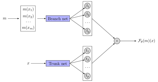
Fig. 2: The framework of DeepOnet.

After the operator network has been trained, an approximation of the forward model $\mathcal{G}$ can be constructed by adding the observation operator $\mathcal{O}$, i.e., $\widehat{\mathcal{G}}=\mathcal{O}\circ\mathcal{F}_{\theta}$. We then can obtain the surrogate posterior

$$\widehat{\nu}(dm)\propto\exp(-\widehat{\Phi}(m;y))\nu_{0}(dm),$$

where $\nu_{0}$ is again the prior of $m$ and $\widehat{\Phi}(m;y)$ is the approximate least-squares data misfit defined as

$$\widehat{\Phi}(m;y):=\frac{1}{2}\left\|y-\widehat{\mathcal{G}}(m)\right\|^{2}_{\Sigma_{\eta}}.$$

The main advantage of the surrogate method is that once an accurate approximation is obtained, it can be evaluated many times without resorting to additional simulations of the full-order forward model. However, using approximate models directly may introduce a discrepancy or modeling error, exacerbating an already ill-posed problem and leading to a worse solution[15]. Specifically, we can define an $\epsilon$-feasible set $\mathcal{M}(\epsilon):=\{m\in\mathcal{M}|\|\mathcal{G}(m)-\widehat{\mathcal{G}}(m)\|\leq\epsilon\},$ and the associated posterior measure $\nu(\mathcal{M}(\epsilon))$ as

$$\nu(\mathcal{M}(\epsilon))=\int_{\mathcal{M}(\epsilon)}\nu(dm).$$

Then, the complement of the $\epsilon$-feasible set is given by $\mathcal{M}^{\bot}(\epsilon)=\mathcal{M}\setminus\mathcal{M}(\epsilon)$, which has posterior measure $\nu(\mathcal{M}^{\bot}(\epsilon))=1-\nu(\mathcal{M}(\epsilon))$. We can obtain an error bound between $\widehat{\nu}$ and $\nu$ in the Kullback-Leibler distance:

Theorem 1 ([40]).

Suppose we have the full posterior distribution $\nu$ and its approximation $\widehat{\nu}$ induced by the surrogate $\widehat{\mathcal{G}}$. For a given $\epsilon$, there exist constants $K_{1}>0$ and $K_{2}>0$ such that

$$D_{KL}(\nu\|\widehat{\nu})\leq\Big{(}K_{1}\epsilon+K_{2}\nu(\mathcal{M}^{\bot}(\epsilon))\Big{)}^{2}.$$

It is important to note that in order for the approximate posterior $\widehat{\nu}$ to converge to the exact posterior $\nu$, the posterior measure $\nu(\mathcal{M}^{\bot}(\epsilon))$ must tend to zero. One way to achieve this goal is to enable the surrogate model $\widehat{\mathcal{G}}$ trained sufficiently in the entire input space such that the model error is small enough. However, a significant amount of data and training time are frequently required to effectively train the surrogate model. Indeed, the surrogate model only needs to be accurate within the posterior distribution space, not the entire prior space[33, 15, 40]. To maintain accurate results while lowering the computational costs, an adaptive algorithm should be developed. In the following section, we will examine how to create a framework for adaptively reducing the modeling error of the surrogate. Typically, we start by building a surrogate offline with DeepOnet. We then propose employing a greedy algorithm to adaptively update the training dataset in order to reduce the model error, after which the pre-trained surrogate can be fine-tuned online.

3 Adaptive operator learning framework

3.1 Adaptive model error reduction

Standard DeepOnet requires a large set of training points, which are obtained through solving time-consuming forward model. This is not practical and will also introduce model error in most cases. To address this challenge, one possible way is to use a locally accurate surrogate to replace the forward model and then explore the approximate posterior distribution induced by this surrogate. In detail, suppose we have a collection of model evaluations $\mathcal{D}=\{(m_{i},\mathcal{F}(m_{i}))\}$. We then can use these points to train an operator network $\mathcal{F}_{\theta}$ and obtain a surrogate $\widehat{\mathcal{G}}=\mathcal{O}\circ\mathcal{F}_{\theta}$, which can be evaluated repeatedly at negligible cost, making it ideal for drawing samples from posterior distributions.

It should be noticed that the training dataset influences the accuracy of the approximation model. If given sufficient training points, the surrogate model $\widehat{\mathcal{G}}$ will be accurate in the whole prior space. While this is not practical and will lost the advantage of computational efficiency [15, 40]. Moreover, how to choose the training points can still be a challenge as one needs to make sure the accuracy of the surrogate in the high posterior density region. However, the high density region of the posterior distribution is unknown until the observations are given. Therefore, we need to design an algorithm that can modify the training dataset during the posterior computational process to fine-tune the pre-trained surrogate. This refined surrogate can maintain the local accuracy as well as save computational cost.

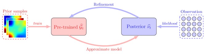
Fig. 3: The flowchart of our framework.

Our approach, as depicted in Fig.3 is indeed the summary of the previous efforts. The whole procedure can be divided into the following four steps.

• Step 1 (Offline): Build a surrogate $\mathcal{F}_{\theta}$ using the initial training dataset $\mathcal{D}$ with a relatively small sample size.

• Step 2 (Posterior computation): Using some numerical techniques to approximate, or draw samples from the approximate posterior $\widehat{\nu_{t}}$ induced by $\widehat{\mathcal{G}}_{t}=\mathcal{O}\circ\mathcal{F}_{\theta}$.

• Step 3 (Refinement): Choose a criteria to determine whether the refinement if needed. If refinement is needed, then selecting new points from $\widehat{\nu_{t}}$ to refine the training dataset $\mathcal{D}$ and the surrogate $\mathcal{F}_{\theta}$.

• Step 4: Repeated the above procedure for many times until the stop criteria is satisfied.

Once the initial model has been trained, a rough inversion result can be obtained for different inversion tasks at a negligible cost by using this pre-trained model. The operator network is then fine-tuned online using our adaptive framework to improve the inversion results. The remaining challenges are to define the stop criteria and the sampling technique for choosing adaptive points from $\widehat{\nu}_{t}$. To construct the stop criteria, we use the least squares functional $\Phi(m;y)$ as the error term because it represents the relative distance between the observations and the forward predictions. In detail, suppose

$$e_{t}=\Phi(r_{t};y)=\frac{1}{2}\|y-\mathcal{G}(r_{t})\|_{\Sigma_{\eta}}^{2}.$$ (4)

By giving a predefined tolerance $\epsilon$, if $\frac{e_{t}-e_{t+1}}{e_{t}}<\epsilon$, the whole procedure should be stopped as the data-fitting term does not decrease significantly anymore. While for the sampling technique, in order to maintain efficiency, we need to choose a small set of samples based on current posterior $\widehat{\nu}_{t}$. In detail, we need to first generate a large set of samples from $\widehat{v}_{t}$ and then choose a couple of important samples based on some criteria. To this end, a natural idea is to combine the numerical techniques used in posterior computation and a greedy algorithm to adaptively choose the most important samples from $\widehat{\nu}_{t}$.

Suppose the current approximate posterior distribution is $\widehat{\nu}_{t}$, we need to generate samples from it to retrain the pre-trained model $\mathcal{F}_{\theta}$. To select the small set of important parameter points, we first draw a large set of $K$ samples $\Gamma=\{m_{1},m_{2},\cdots,m_{K}\}$ from $\widehat{\nu}_{t}$ to cover the parameter space. A subset $\gamma^{Q}=\{\widetilde{m}_{1},\widetilde{m}_{2},\cdots,\widetilde{m}_{Q}\}\subset\Gamma$ of ”important” points are selected from $\Gamma$ using a Greedy algorithm. That is, we firstly select the current mean vector $r_{t}$ as the anchor point, which can be estimated by samples mean in general cases. Afterwards, we want the newly selected point $\widetilde{m}_{j}$ to be close to $r_{t}$. And at the same time, the surrogate solution of this point should have the largest distance with the space spanned by $\{\widehat{\mathcal{G}}_{t}(\widetilde{m}_{i})\}_{i=1}^{j-1}$, i.e.,

$$\begin{split}&\widetilde{m}_{j}=\arg\max_{m\in\Gamma/\gamma^{j-1}}\left(d\big{(}\widehat{\mathcal{G}}_{t}(m),\widehat{\mathcal{G}}_{t}(\gamma^{j-1})\big{)}-d(m,r_{t})\right),\\ &\gamma^{j}=\gamma^{j-1}\cup\{\widetilde{m}_{j}\},\end{split}$$ (5)

where $d(\mathbf{x},\mathbf{y})$ is the distance function between vector $\mathbf{x}$ and $\mathbf{y}$, which is defined by $l_{2}$ norm. $\widehat{\mathcal{G}}_{t}(\gamma^{j-1})$ represents the space spanned by $\{\widehat{\mathcal{G}}_{t}(\widetilde{m}_{i})\}_{i=1}^{j-1}$.

The purpose of this strategy is to keep the adaptive points closing to the mean vector. Specifically, the selected adaptive points will contain the varying features in the surrogate solution spaces and will be in close proximity to the mean vector $r_{t}$. These points then allow the pre-trained model to be fine-tuned to be more accurate near $r_{t}$ and to show better generalization ability. The important thing is to sample from the approximate posterior distribution and approximate the mean vector. To this end, traditional MCMC-based sampling methods can be applied. However, the slow convergence rate of MCMC methods, which always require $\mathcal{O}(10^{5})$ iterations, has led to widespread criticism in practice, even though they possess attractive asymptotic theoretical properties. Particle-based approaches[41, 42, 43, 44, 45], particularly Kalman-based Bayesian inversion techniques[46, 47, 48, 49, 43, 50, 51, 52, 53], have been proposed recently to bridge the gap between MCMC and VI techniques. We investigate the unscented Kalman inversion (UKI) method[35] in this paper because it never needs early stopping or empirical variance inflation, and it converges with only $\mathcal{O}(10)$ iterations. Notably, our framework is easily extensible to numerous variants of popular particle-based methods; however, this is outside the scope of this work.

3.2 Unscented Kalman Inversion

In this section, we give a brief review of the UKI algorithm discussed in [35]. The UKI is derived within the Bayesian framework and is considered to approximate the posterior distribution using Gaussian approximations on the random variable $m|y$ via its ensemble properties. To this end, we consider the following stochastic dynamical system:

$$\begin{split}&\text{Evolution:}\quad\quad m_{n+1}=r_{0}+\alpha(m_{n}-r_{0})+\omega_{n+1},\quad\quad\omega_{n+1}\sim\mathcal{N}(0,\Sigma_{\omega}),\\ &\text{Observation:}\quad\quad y_{n+1}=\mathcal{G}(m_{n+1})+\eta_{n+1},\quad\quad\quad\quad\quad\eta_{n+1}\sim\mathcal{N}(0,\Sigma_{\eta}).\end{split}$$ (6)

where $m_{n+1}$ is the unknown discrete parameter vector, and $y_{n+1}$ is the observation vector, the artificial evolution error $\omega_{n+1}$ and observation error $\eta_{n+1}$ are mutually independent, zero-mean Gaussian sequences with covariances $\Sigma_{\omega}$ and $\Sigma_{\eta}$, respectively. Here $\alpha\in(0,1]$ is the regularization parameter, $r_{0}$ is the initial arbitrary vector.

Let $Y_{n}:=\{y_{1},y_{2},\cdots,y_{n}\}$ denotes the observation set at time $n$. In order to approximate the conditional distribution $\nu_{n}$ of $m_{n}|Y_{n}$, the iterative algorithm starts from the prior $\nu_{0}$ and updates $\nu_{n}$ through the prediction and analysis steps: $\nu_{n}\rightarrow\widehat{\nu}_{n+1}$, and then $\widehat{\nu}_{n+1}\rightarrow\nu_{n+1}$, where $\widehat{\nu}_{n+1}$ is the distribution of $m_{n+1}|Y_{n}$. In the prediction step, we assume that $\nu_{n}=\mathcal{N}(r_{n},C_{n})$, then under Eq. (6), $\widehat{\nu}_{n+1}$ is also Gaussian with mean and covariance:

$$\begin{split}&\widehat{r}_{n+1}=\mathbb{E}[m_{n+1}|Y_{n}]=\alpha r_{n}+(1-\alpha)r_{0},\\ &\widehat{C}_{n+1}={\mathrm{Cov}}[m_{n+1}|Y_{n}]=\alpha^{2}C_{n}+\Sigma_{\omega}.\end{split}$$ (7)

In the analysis step, we assume that joint distribution of $\{m_{n+1},y_{n+1}\}|Y_{n}$ can be approximated by a Gaussian distribution

$$\mathcal{N}\left(\left[\begin{array}[]{c}\widehat{r}_{n+1}\\ \widehat{y}_{n+1}\end{array}\right],\left[\begin{array}[]{cc}\widehat{C}_{n+1}&\widehat{C}^{my}_{n+1}\\ {\widehat{C}_{n+1}^{my\;T}}&\widehat{C}_{n+1}^{yy}\end{array}\right]\right),$$ (8)

where

$$\begin{array}[]{l}{{\widehat{y}_{n+1}=\mathbb{E}[{\mathcal{G}}(m_{n+1})|Y_{n}],}}\\ {{\widehat{C}_{n+1}^{my}=\operatorname{Cov}[m_{n+1},{\mathcal{G}}(m_{n+1})|Y_{n}],}}\\ {{\widehat{C}_{n+1}^{yy}=\operatorname{Cov}[{\mathcal{G}}(m_{n+1})|Y_{n}]+\Sigma_{\eta}.}}\end{array}$$ (9)

Conditioning the Gaussian in Eq.(8) to find $m_{n+1}|\{Y_{n},y_{n+1}\}=m_{n+1}|Y_{n+1}$ gives the following expressions for the mean $r_{n+1}$ and covariance $C_{n+1}$ of the approximation to $\nu_{n+1}$:

$$\begin{array}[]{l l}{{r_{n+1}=\widehat{r}_{n+1}+\widehat{C}_{n+1}^{my}(\widehat{C}_{n+1}^{yy})^{-1}(y_{n+1}-\widehat{y}_{n+1}),}}\\ {{C_{n+1}=\widehat{C}_{n+1}-\widehat{C}_{n+1}^{my}(\widehat{C}_{n+1}^{yy})^{-1}\widehat{C}_{n+1}^{my}}}.\end{array}$$ (10)

By assuming all observations are identical to $y$ (i.e., $Y_{n}=y$), Eqs.(7)-(10) define a conceptual algorithm for using Gaussian approximation to solve BIPs. To evaluate integrals appearing in Eq. (7), UKI employs the unscented transform described below.

Theorem 2 (Modified Unscented Transform [54]).

Let Gaussian random variable $m\sim\mathcal{N}(r,C)\in\mathbb{R}^{N_{m}}$, $2N_{m}+1$ symmetric $\sigma$-points are chosen deterministically:

$$m^{0}=r,\quad m^{j}=m+c_{j}[\sqrt{C}]_{j},\quad m^{j+N_{m}}=m-c_{j}[\sqrt{C}]_{j},\quad(1\leq j\leq N_{m}),$$

where $[\sqrt{C}]_{j}$ is the $jth$ column of the Cholesky factor of $C$. The quadrature rule approximates the mean and covariance of the transformed variable $\mathcal{G}_{i}(m)$ as follows

$$\begin{split}&\mathbb{E}[\mathcal{G}_{i}(\theta)]\approx\mathcal{G}_{i}(m_{0})=\mathcal{G}_{i}(r),\\ &Cov[{\mathcal{G}_{1}}(m),\mathcal{G}_{2}(m)]\approx\sum_{i=1}^{2N_{m}}W_{j}^{c}\left(\mathcal{G}_{1}(m^{j})-\mathbb{E}{\mathcal{G}_{1}}(m)\right)\left(\mathcal{G}_{2}(m^{j})-\mathbb{E}{\mathcal{G}_{2}}(m)\right)^{T}.\end{split}$$

Here these constant weights are

$$\begin{split}&c_{1}=c_{2}\cdots=c_{N_{m}}=\sqrt{N_{m}+\lambda},\quad W_{1}^{c}=W_{2}^{c}=\cdots=W_{2N_{m}}^{c}=\frac{1}{2(N_{r}+\lambda)},\\ &\lambda=a^{2}(N_{m}+\kappa)-N_{m},\quad\kappa=0,\quad a=\min\{\sqrt{\frac{4}{N_{m}+\kappa}},1\}.\end{split}$$

We obtain the following UKI algorithm in Algorithm 1 by applying the aforementioned quadrature rules. UKI is a derivative-free algorithm that applies a Gaussian approximation theorem iteratively to transport a set of particles to approximate given distributions. As a result, it only needs $2N_{m}+1$ forward evaluations per iteration, making it simple to implement and inexpensive to compute.

Algorithm 1 Unscented Kalman Inversion (UKI)

1:procedure RunUki($r_{0},C_{0},y,\mathcal{G},\Sigma_{\omega},\Sigma_{\eta},T$)

2:     for $n=0,\ldots,T-1$ do

3:         Prediction step:

$$\widehat{r}_{n+1}=\alpha r_{n}+(1-\alpha)r_{0},\widehat{C}_{n+1}=\alpha^{2}C_{n}+\Sigma_{\omega}.$$

4:         Generate $\sigma$-points

$$\begin{split}&\widehat{m}^{0}_{n+1}=\widehat{r}_{n+1},\\ &\widehat{m}^{j}_{n+1}=\widehat{r}_{n+1}+c_{j}[\sqrt{\widehat{C}_{n+1}}]_{j},\quad(1\leq j\leq N_{m}),\\ &\widehat{m}^{j+N_{m}}_{n+1}=\widehat{r}_{n+1}-c_{j}[\sqrt{\widehat{C}_{n+1}}]_{j},\quad(1\leq j\leq N_{m}).\end{split}$$

5:         Analysis step:

$$\begin{split}&\widehat{s}_{n+1}^{j}=\mathcal{G}(\widehat{m}_{n+1}^{j}),\qquad\widehat{y}_{n+1}=\widehat{y}_{n+1}^{0},\\ &\widehat{C}_{n+1}^{my}=\sum_{j=1}^{2N_{m}}W_{j}^{c}(\widehat{m}_{n+1}^{j}-\widehat{r}_{n+1})(\widehat{y}_{n+1}^{j}-\widehat{y}_{n+1})^{T},\\ &\widehat{C}_{n+1}^{yy}=\sum_{j=1}^{2N_{m}}W_{j}^{c}(\widehat{y}_{n+1}^{j}-\widehat{y}_{n+1})(\widehat{y}_{n+1}^{j}-\widehat{y}_{n+1})^{T}+\Sigma_{\eta},\\ &r_{n+1}=\widehat{r}_{n+1}+\widehat{C}_{n+1}^{my}(\widehat{C}_{n+1}^{yy})^{-1}(y-\widehat{y}_{n+1}),\\ &C_{n+1}=\widehat{C}_{n+1}-\widehat{C}_{n+1}^{my}(\widehat{C}_{n+1}^{yy})^{-1}\widehat{C}_{n+1}^{my}\end{split}$$

6:     end for

7:end procedure

3.3 Algorithm Summary

Algorithm 2 UKI with DeepOnet approximation

1:procedure RunLUki($\mathcal{D},\mathcal{F},\mathcal{F}_{\theta},y,r_{0},C_{0},\Sigma_{\omega},\Sigma_{\eta},T,I_{\max},\epsilon$)

2:     Set $\widehat{\mathcal{G}}_{0}=\mathcal{O}\circ\mathcal{F}_{\theta}$, and compute $e_{0}$ using Eq.(4).

3:     for $t=0,\ldots,I_{max}-1$ do

4:         $(r_{t+1},C_{t+1},e_{t+1})\leftarrow$ RunUki($r_{t},C_{t},y,\widehat{\mathcal{G}}_{t},\Sigma_{\omega},\Sigma_{\eta},T$)

5:         if $(e_{t}-e_{t+1})/e_{t}>\epsilon$ then

6:              ($\widehat{\mathcal{G}}_{t+1},\mathcal{D})\leftarrow$RefineApprox($r_{t+1},C_{t+1},\mathcal{D},\mathcal{F},\mathcal{F}_{\theta}$)

7:         end if

8:     end for

9:end procedure

10:

11:procedure RefineApprox($r,C,\mathcal{D},\mathcal{F},\mathcal{F}_{\theta}$)

12:     Sample $\Gamma=\{m_{j}\}_{j=1}^{K}\sim\mathcal{N}(r,C)$.

13:     Choose new $Q$ samples $\widetilde{m}_{j}$ using Eq. (5), and grow $\mathcal{D}\leftarrow\mathcal{D}\cup\{\widetilde{m}_{j},\mathcal{F}(\widetilde{m}_{j})\}$

14:     Update the operator network $\mathcal{F}_{\theta}$ using the training set $\mathcal{D}$

15:     return the surrogate $\widehat{\mathcal{G}}=\mathcal{O}\circ\mathcal{F}_{\theta}$ and the training set $\mathcal{D}$

16:end procedure

Algorithm 2 provides an overview of the UKI method utilizing DeepOnet approximations. The algorithm works in a manner similar to how our adaptive operator framework is explained. In summary, we begin with an offline pre-trained DeepOnet surrogate and use locally training data from the current approximate posterior distribution to adaptively refine this DeepOnet until the stop criteria is met. It is important to note that the UKI iteration process with DeepOnet may not always be stable. Therefore, in order to get the final approximate posterior distribution in each refinement, we run the UKI for $T$ steps and select the mean vector whose data fitting error is the smallest as the output. Consequently, more $T$ forward evaluations are needed for each refinement in this process.

We review the computational efficiency of our method. Since the pre-trained operator network can be applied as surrogates for a class of various BIPs with models that are governed by the same PDEs but have various types of observations and noise modes. Thus, for a given inversion task, the main computational cost centers on the online forward evaluations and the online fine-tuning. On the other hand, the online retraining only takes a few seconds each time, so it can be ignored in comparison to the forward evaluation time. In these situations, the forward evaluations account for the majority of the computational cost. For our algorithm, the maximum number of online high-fidelity model evaluations is $N_{DeepOnet}=\sum_{t=1}^{I_{max}}(Q+T_{\tiny{DeepOnet}})=(Q+T_{\tiny{DeepOnet}})I_{max}$, where $Q$ is the number of adaptive samples for refinement, $T_{\tiny{DeepOnet}}$ is the maximum number of iterations for UKI using our approach, and $I_{max}$ is the number of adaptive refinement. While $N_{\tiny{FEM}}=(2N_{m}+1)T_{\tiny{FEM}}$ represents the total evaluations for UKI using the FEM solver, $N_{m}$ represents the discrete dimension of the parameter field, and $T_{FEM}$ represents the maximum iteration number for UKI. Consequently, the asymptotic speeds increase can be computed as

$$SpeedUp=\frac{(2N_{m}+1)T_{\tiny{FEM}}}{(Q+T_{\tiny{DeepOnet}})I_{max}}.$$

Note that the efficiency of our method basically depends on $Q,I_{max}$. First of all, the number of adaptive samples $Q$ will be sufficiently small (e.g. $\mathcal{O}(10)$) compared to the discrete dimension $N_{m}$ (e.g. $\mathcal{O}(10^{2})-\mathcal{O}(10^{3})$), resulting in a significant reduction in computational cost as it determines the number of forward evaluations. Second, the total number of adaptive retraining $I_{max}$ is determined by the inverse tasks, which are further subdivided into in-distribution data (IDD) and out-of-distribution (OOD) cases. The IDD typically refers to ground truth that is located in the high density region of the prior distribution. Alternatively, the OOD refers to the ground truth that is located far from the high density area of the prior. The original pre-trained surrogate can be accurate in nearly all of the high probability areas for the IDD case. As a result, our framework will converge quicker. In the case of OOD, our framework requires a significantly higher number of retraining cycles in order to reach the high density area of the posterior distribution. However $I_{max}$ for both inversion tasks can be small. Consequently, our method can simultaneously balance accuracy and efficiency and has the potential to be applied to dynamical inversion tasks. In other words, once the initial surrogate is trained, we can use our adaptive framework to modify the estimate at a much lower computational cost.

3.4 Convergence analysis under the linear case

It is important to note that the UKI’s ensemble properties are used to approximate the posterior distribution using Gaussian approximations. Specifically, the sequence in Eq.(10) obtained by the full-order model $\mathcal{G}$ will converge to the equilibrium points of the following equations under certain mild conditions in the linear case [35]:

$$C_{\infty}^{-1}=\mathcal{G}^{T}\Sigma_{\eta}^{-1}\mathcal{G}+(\alpha^{2}C_{\infty}+\Sigma_{\omega})^{-1},$$ (11a)

$$C_{\infty}^{-1}r_{\infty}=\mathcal{G}^{T}\Sigma_{\eta}^{-1}y+(\alpha^{2}C_{\infty}+\Sigma_{\omega})^{-1}\alpha r_{\infty}.$$ (11b)

We can actually demonstrate that in the linear case, the mean vector and covariance matrix obtained by our approach will be near to those obtained by the true forward if the surrogate $\widehat{\mathcal{G}}$ is near to the true forward $\mathcal{G}$. Consider the following: $\mathop{\operator@font Range}\nolimits(\widehat{\mathcal{G}})=\mathbb{R}^{N_{m}}$, and $\widehat{\mathcal{G}}$ is linear. Using $\widehat{\mathcal{G}}$ as a surrogate, the corresponding sequence of $r_{n},C_{n}$ in Eq.(10) then converges to the following equations

$$\widehat{C}_{\infty}^{-1}=\widehat{\mathcal{G}}^{T}\Sigma_{\eta}^{-1}\widehat{\mathcal{G}}+(\alpha^{2}\widehat{C}_{\infty}+\Sigma_{\omega})^{-1},$$ (12a)

$$\widehat{C}_{\infty}^{-1}\widehat{r}_{\infty}=\widehat{\mathcal{G}}^{T}\Sigma_{\eta}^{-1}y+(\alpha^{2}\widehat{C}_{\infty}+\Sigma_{\omega})^{-1}\alpha\widehat{r}_{\infty}$$ (12b)

In the following, we will demonstrate that if the surrogate $\widehat{\mathcal{G}}$ is near the true forward model $\mathcal{G}$, then the $\widehat{r}_{\infty},\widehat{C}_{\infty}$ ought to be near the true ones as well. We shall need the following assumptions.

Assumption 3.

Suppose for any $\epsilon$, the linear neural operator $\widehat{\mathcal{G}}:\mathbb{R}^{N_{m}}\rightarrow\mathbb{R}^{N_{y}}$ can be trained sufficiently to satisfy

$$\|\widehat{\mathcal{G}}-\mathcal{G}\|_{2}<\epsilon.$$ (13)

Assumption 4.

Suppose the forward map $\mathcal{G}$ is bounded, that is

$$\|\mathcal{G}\|_{2}<H,$$ (14)

where $H$ is a constant.

Assumption 5.

Suppose the matrix $\mathcal{G}^{T}\Sigma_{\eta}^{-1}\mathcal{G}\succ 0$ and can be bounded from below as

$$\|\mathcal{G}^{T}\Sigma_{\eta}^{-1}\mathcal{G}\|_{2}>C_{1},$$ (15)

where $C_{1}$ is a positive constant.

We can obtain the following lemma.

Lemma 6.

Under Assumptions 3-5, $\widehat{\mathcal{G}}^{T}\Sigma_{\eta}^{-1}\widehat{\mathcal{G}}$ is also bounded from below as

$$\|\widehat{\mathcal{G}}^{T}\Sigma_{\eta}^{-1}\widehat{\mathcal{G}}\|_{2}>C_{2}.$$ (16)

where $C_{2}$ is constant dependent on $C_{1}$.

Proof.

We first consider

$$\begin{split}\mathcal{G}^{T}\Sigma_{\eta}^{-1}\mathcal{G}-\widehat{\mathcal{G}}^{T}\Sigma_{\eta}^{-1}\widehat{\mathcal{G}}&=\mathcal{G}^{T}\Sigma_{\eta}^{-1}\mathcal{G}-\mathcal{G_{\theta}}^{T}\Sigma_{\eta}^{-1}\mathcal{G}+\mathcal{G_{\theta}}^{T}\Sigma_{\eta}^{-1}\mathcal{G}-\widehat{\mathcal{G}}^{T}\Sigma_{\eta}^{-1}\widehat{\mathcal{G}}\\ &=\left(\mathcal{G}-\widehat{\mathcal{G}}\right)^{T}\Sigma_{\eta}^{-1}\mathcal{G}+\mathcal{G_{\theta}}^{T}\Sigma_{\eta}^{-1}\left(\mathcal{G}-\widehat{\mathcal{G}}\right).\end{split}$$ (17)

Combining Assumptions 3 and 4, this leads to

$$\begin{split}\|\mathcal{G}^{T}\Sigma_{\eta}^{-1}\mathcal{G}-\widehat{\mathcal{G}}^{T}\Sigma_{\eta}^{-1}\widehat{\mathcal{G}}\|_{2}&\leq\|\mathcal{G}-\widehat{\mathcal{G}}\|_{2}\|\Sigma_{\eta}^{-1}\|_{2}(\|\mathcal{G}\|_{2}+\|\widehat{\mathcal{G}}\|_{2})\\ &\leq 2\epsilon H\|\Sigma_{\eta}^{-1}\|_{2}.\end{split}$$ (18)

Then, we have

$$\begin{split}\|\widehat{\mathcal{G}}^{T}\Sigma_{\eta}^{-1}\widehat{\mathcal{G}}\|_{2}&=\|\widehat{\mathcal{G}}^{T}\Sigma_{\eta}^{-1}\widehat{\mathcal{G}}-\mathcal{G}^{T}\Sigma_{\eta}^{-1}\mathcal{G}+\mathcal{G}^{T}\Sigma_{\eta}^{-1}\mathcal{G}\|_{2}\\ &\geq\|\mathcal{G}^{T}\Sigma_{\eta}^{-1}\mathcal{G}\|_{2}-\|\widehat{\mathcal{G}}^{T}\Sigma_{\eta}^{-1}\widehat{\mathcal{G}}-\mathcal{G}^{T}\Sigma_{\eta}^{-1}\mathcal{G}\|_{2}\\ &\geq C_{1}-2\epsilon H\|\Sigma_{\eta}^{-1}\|_{2}\geq C_{2}.\end{split}$$ (19)

∎

Note that these assumptions are reasonable and can be found in many references [14, 33]. We will then supply the main theorem based on these assumptions.

Theorem 7.

Under Assumptions 3-5, suppose $Range(\mathcal{G}^{T})=Range(\widehat{\mathcal{G}}^{T})=\mathbb{R}^{N_{m}}$ and $\Sigma_{\omega}\succ 0,\Sigma_{\eta}\succ 0$. Then the sequence $\widehat{r}_{\infty},\widehat{C}_{\infty}^{-1}$ in Eq.(12) obtained by using the surrogate model will converge to the $r_{\infty},C_{\infty}^{-1}$ in Eq.(11) and we have the following error estimate

$$\begin{split}&\|C_{\infty}^{-1}-\widehat{C}_{\infty}^{-1}\|_{2}\leq\frac{2\epsilon HH_{\eta}}{1-\beta},\\ &\|r_{\infty}-\widehat{r}_{\infty}\|_{2}\leq\frac{K_{1}H_{\eta}H_{y}}{C_{1}}\left(1+\frac{2(1+\alpha\beta)K_{2}H_{\eta}H^{2}}{(1-\beta)C_{2}}\right)\epsilon,\end{split}$$ (20)

where $\beta,C_{1},C_{2},K_{1},K_{2},H_{\eta},H_{y},H$ are positive bounded constants.

Proof.

The proof can be found in Appendix A.

Remark 1.

In order to meet the requirements of Theorem 7, it is possible to make the neural operator $\mathcal{G}_{\theta}$ linear by dropping the nonlinear activation functions in the branch net and keeping the activation functions in the trunk net.

4 Numerical experiments

In this section, we provide several numerical examples to demonstrate the effectiveness and precision of the adaptive operator learning approach for solving inverse problems. We will compare the UKI inversion results from DeepOnet (referred to as DeepOnet-UKI) and the results from conventional FEM solvers (referred to as FEM-UKI) in order to more clearly present the results. Additionally, there are two cases for the DeepOnet-UKI method: DeepOnet-UKI-Direct and DeepOnet-UKI-Adaptive, depending on whether adaptive refinement is applied.

In all of our numerical tests, the branch and trunk nets for DeepOnet are fully connected neural networks with five hidden layers and one hundred neurons in each layer, with the tanh function as the activation function. DeepOnet is trained offline with $1\times 10^{5}$ iterations and $N_{prior}=1000$ prior samples from the Gaussian random field. Unless otherwise specified, we set the maximum retraining number to $I_{max}=10$ and the tolerance to $\epsilon=0.01$. In order to assess the efficacy of our adaptive model in handling varying observations, we will apply Gaussian random noise of 1%, 5%, and 10% to the observations. This can be expressed as follows:

$$y_{obs}=y_{ref}+\delta\odot\xi,\xi\sim\mathcal{N}(0,1),$$ (21)

where $y_{ref}=\mathcal{G}(m_{ref}),\delta=1\%y_{ref},\delta=5\%y_{ref},\delta=10\%y_{ref}$ and $\odot$ denotes the element-wise multiplication. In UKI, the regularization parameters are $\alpha=0.5$ for noise levels 0.05 and 0.1 and $\alpha=1$ for noise levels 0.01. The starting vector for the UKI is chosen at random from $\mathcal{N}(0,I)$. The selection of other hyper-parameters is based on [35]. For numerical examples, we set $\Omega=[0,1]^{2}$. The maximum number of UKI iterations in a retraining cycle is 20 for all three methods. After that, we will choose $Q=50$ adaptive samples for noise level 0.01 and $Q=20$ adaptive samples for noise levels 0.05 and 0.1, respectively, from 2000 samples using the greedy algorithm.

To measure the accuracy of the numerical approximation with respect to the exact solution, we use the following relative error $err$ defined as

$$err=\frac{\|\widehat{m}-m_{ref}\|_{2}}{\|m_{ref}\|_{2}},$$ (22)

where $\widehat{m}$ and $m_{ref}$ are the numerical and exact solutions , respectively. Furthermore, in order to compare the model error, we define the relative model error as follows:

$$Err=\frac{\|\widehat{\mathcal{G}}(\widehat{m})-\mathcal{G}(\widehat{m})\|_{2}}{\|\mathcal{G}(\widehat{m})\|_{2}}.$$ (23)

4.1 Example 1: Darcy flow

In the first example, we consider the following Darcy flow problem:

$$\begin{split}-\nabla\cdot(\exp(\mathbf{m}(\mathbf{x}))\nabla{u(\mathbf{x})})&=f(\mathbf{x}),\quad\mathbf{x}\in\Omega,\\ u(\mathbf{x})&=0,\quad\quad\mathbf{x}\in\partial\Omega.\end{split}$$ (24)

Here, the source function $f(\mathbf{x})$ is defined as

$$f(x_{1},x_{2})=\begin{cases}1000\quad 0\leq x_{2}\leq\frac{4}{6},\\ 2000\quad\frac{4}{6}<x_{2}\leq\frac{5}{6},\\ 3000\quad\frac{5}{6}<x_{2}\leq 1.\end{cases}$$ (25)

The aim is to determine the permeability $\mathbf{m}(\mathbf{x})$ from noisy measurements of the $u$-field at a finite set of locations. To ensure the existence of the posterior distribution, we typically selected the prior distribution $\nu_{0}$ as a Gaussian measure $\mathcal{N}(r_{pr},\mathcal{C}_{pr})$. In particular, we focus on the covariance operator with the following form:

$$\mathcal{C}_{pr}=\sigma^{2}(-\Delta+\tau^{2})^{-d},$$ (26)

where $\Delta$ denotes the Laplacian operator in $\Omega$ subject to homogeneous Neumann boundary conditions, $\tau$ denotes the inverse length scale of the random field and $d>0$ determines its regularity. For the numerical experiments presented in this section, we take the same values for these parameters as in[35]: $\tau=3,d=2,\sigma=1$. To sample from the prior distribution, we can use the Karhunen-Loeve (KL) expansion , which has the form

$$\mathbf{m}(\mathbf{x})=\sum_{k\in\mathbb{Z}^{+}}\theta_{k}\sqrt{\lambda_{k}}\psi_{k}(\mathbf{x}),$$ (27)

where $\lambda_{k}$ and $\psi_{k}$ are the eigenvalues and eigenfunctions, and $\theta_{k}\sim\mathcal{N}(0,1)$ are independent random variables. In practice, we truncate the sum (27) to $n_{d}$ terms, based on the largest $n_{d}$ eigenvalues, and hence $\theta\in\mathbb{R}^{n_{d}}$. The forward problem is solved by FEM method on a $70\times 70$ grid.

We will create the observation data for the inverse problem using the in-distribution data (IDD) and out-of-distribution data (OOD), respectively, as shown in Fig.4. The IDD field $\mathbf{m}_{ref}(\mathbf{x})$ is calculated using (27) with $n_{d}=256$ and $\theta_{k}\sim\mathcal{N}(0,1)$. The OOD field $\mathbf{m}_{ref}(\mathbf{x})$ is generated for convenience by sampling $\theta_{k}\sim\mathcal{U}[-20,20],k=1,\ldots,256$. To avoid the inverse crime, we will try to inverse the first $N_{m}=128$ KL modes using these observation data.

\begin{overpic}[width=130.08731pt]{figures/flow2d/true_kappa_in_distribution.png} \end{overpic}

\begin{overpic}[width=133.55437pt]{figures/flow2d/observations_in_distribution.png} \end{overpic}

\begin{overpic}[width=127.9171pt]{figures/flow2d/true_kappa.png} \end{overpic}

\begin{overpic}[width=134.42113pt]{figures/flow2d/observations.png} \end{overpic}

Fig. 4: The ground truth for in-distribution data(IDD) and out-of -distribution data (OOD) from above to below. Left: the true permeability fields $\mathbf{m}(\mathbf{x})$. Right: the pressure fields $u(\mathbf{x})$ and the corresponding $36$ equidistant observations with noise level 0.01.

We plot the retraining loss, model error, and relative error in Fig.5 to illustrate the effectiveness of our framework. When we apply the initial pre-trained model directly to run UKI, we can clearly see in the middle display of Fig.5 that the model error gradually decreases during the iteration for IDD data. Consequently, the relative error for IDD data will be nearly equal to the FEM-UKI value, as shown in the right display of Fig.5. However, for OOD data, the model error will rise sharply, suggesting that the previously trained model will not work as planned. A poorer estimate will result from the simultaneous immediate increase in the relative error for OOD data. Nevertheless, by using an adaptive dataset that arrives at the initial model’s rough estimate, we can enhance the pre-trained model. The left display of Fig.5 shows that the training loss increases initially and then decreases as we refine. As expected, even for OOD data, the model error in Fig.5 continuously decreases with refinement. When combined with our stop criteria, the OOD inversion requires six refinements, compared to the IDD inversion’s four, suggesting a slower rate of convergence. As shown in the right display of Fig.5, for both types of data, the accuracy of the DeepOnet-UKI-Adaptive estimate progressively increased, beginning with the approximative estimate provided by DeepOnet-UKI-Direct. We plot the final estimated permeability fields produced by three different methods in Figs. 6 and 7 for the detailed inversion result. The true permeability field is well approximated by the estimated permeability fields obtained by FEM-UKI and DeepOnet-UKI-Adaptive, but DeepOnet-UKI-Direct’s result differs significantly, further demonstrating the efficacy of our framework.

\begin{overpic}[width=130.08731pt]{figures/flow2d/loss_in_distribution.png} \put(35.0,78.0){\scriptsize{\bf training loss}} \put(16.0,42.0){\footnotesize\bf IDD case} \end{overpic}

\begin{overpic}[width=140.92517pt]{figures/flow2d/model_error_in_distribution.png} \put(38.0,72.0){\scriptsize{\bf model error}} \end{overpic}

\begin{overpic}[width=136.59135pt]{figures/flow2d/err_kappa_in_distribution.png} \put(38.0,75.0){\scriptsize{\bf relative error}} \end{overpic}

\begin{overpic}[width=130.08731pt]{figures/flow2d/loss.png} \put(14.0,42.0){\footnotesize\bf OOD case} \end{overpic}

\begin{overpic}[width=140.92517pt]{figures/flow2d/model_error.png} \end{overpic}

\begin{overpic}[width=134.42113pt]{figures/flow2d/err_kappa.png} \end{overpic}

Fig. 5: The retraining loss (left), relative model error (middle) and relative error (right) for Example 1. Above: IDD case. Below: OOD case.

\begin{overpic}[width=130.08731pt]{figures/flow2d/fem_kappa_in_distribution.png} \put(30.0,88.0){\footnotesize\bf FEM-UKI} \end{overpic}

\begin{overpic}[width=130.08731pt]{figures/flow2d/dnn_kappa_in_distribution.png} \put(8.0,88.0){\footnotesize\bf DeepOnet-UKI-Adaptive} \end{overpic}

\begin{overpic}[width=130.08731pt]{figures/flow2d/direct_kappa_in_distribution.png} \put(10.0,88.0){\footnotesize\bf DeepOnet-UKI-Direct} \end{overpic}

\begin{overpic}[width=132.25092pt]{figures/flow2d/fem_kappa_error_in_distribution.png} \end{overpic}

\begin{overpic}[width=130.08731pt]{figures/flow2d/dnn_kappa_error_in_distribution.png} \end{overpic}

\begin{overpic}[width=130.08731pt]{figures/flow2d/direct_kappa_error_in_distribution.png} \end{overpic}

Fig. 6: IDD case. Above: the estimated permeability field obtained by different methods. Below: the absolute errors with respect the true ones.

\begin{overpic}[width=130.08731pt]{figures/flow2d/fem_kappa.png} \put(30.0,90.0){\footnotesize\bf FEM-UKI} \end{overpic}

\begin{overpic}[width=130.08731pt]{figures/flow2d/dnn_kappa.png} \put(8.0,90.0){\footnotesize\bf DeepOnet-UKI-Adaptive} \end{overpic}

\begin{overpic}[width=130.08731pt]{figures/flow2d/direct_kappa.png} \put(10.0,90.0){\footnotesize\bf DeepOnet-UKI-Direct} \end{overpic}

\begin{overpic}[width=134.42113pt]{figures/flow2d/kappa_fem_error.png} \end{overpic}

\begin{overpic}[width=130.08731pt]{figures/flow2d/kappa_dnn_error.png} \end{overpic}

\begin{overpic}[width=127.9171pt]{figures/flow2d/kappa_direct_error.png} \end{overpic}

Fig. 7: OOD case. Above: the estimated permeability field obtained by different methods. Below: the absolute errors with respect the true ones.

\begin{overpic}[width=176.05225pt]{figures/flow2d/err_comparison_in_distribution_points.png} \put(40.0,76.0){\footnotesize\bf IDD case} \end{overpic}

\begin{overpic}[width=173.44534pt]{figures/flow2d/err_comparison_points.png} \put(40.0,77.0){\footnotesize\bf OOD case} \end{overpic}

Fig. 8: The error box plot of $err_{DeepOnet}-err_{FEM}$ with increasing adaptive points for the flow case. Left: the relative errors for IDD inversion. Right: the relative errors for the OOD inversion. Current noise level is 0.01.

\begin{overpic}[width=151.76964pt]{figures/flow2d/err_comparison_in_comparison.png} \put(40.0,78.0){\footnotesize\bf IDD case} \end{overpic}

\begin{overpic}[width=153.93324pt]{figures/flow2d/err_comparison.png} \put(40.0,78.0){\footnotesize\bf OOD case} \end{overpic}

\begin{overpic}[width=156.10345pt]{figures/flow2d/num_forward_in_distribution.png} \end{overpic}

\begin{overpic}[width=156.10345pt]{figures/flow2d/num_forward.png} \end{overpic}

Fig. 9: Above: the error box plot of $err_{DeepOnet}-err_{FEM}$ for IDD inversion and OOD inversion. Below: the mean total number of forward evaluations for FEM-UKI and DeepOnet-UKI-Adaptive respectively.

We repeat the experiment ten times for each $Q\in[20,50,100,150]$ to test the impact of the number $Q$ of adaptive samples used in each refinement. The error box of $err_{DeepOnet}-err_{FEM}$ is plotted in Fig.8. It is evident from the IDD data that the relative error does not decrease significantly with increasing data. This suggests that a small set of adaptive samples– roughly 50 – can meet the requirements for accuracy and efficiency. On the other hand, the relative error for OOD data steadily drops with increasing dataset size.

In order to demonstrate the computational cost and examine the effects of varying noise levels, we are going to perform the experiment with three different noise levels (0.01, 0.05, and 0.1) and then repeat it with ten different UKI initial values. The numerical results are shown in Fig.9. We can clearly observe that the relative error gradually drops as noise levels rise, suggesting that higher noise levels are less sensitive to model errors. Consequently, our framework performs better in real-world applications with higher noise levels. We plot the mean total online forward evaluations in Fig.9 to show the computational cost. It is evident that our method has a very small cost in comparison to conventional numerical methods, even with adaptive refinement. This is due to the fact that, unlike FEM-UKI, which requires 257 forward evaluations, we only need a maximum of 50 samples to refine the model each time. The online fine-tuning cost is negligible when compared to the expensive online forward simulations, as retraining only takes a few seconds each time.

4.2 Example 2: The heat source inversion problem

Consider the following heat conduction problem in $\Omega$

$$u_{t}(\mathbf{x})-\Delta u(\mathbf{x}) =f(\mathbf{x},t), \text{ in }\Omega\times[0,1],$$ (28)

$$u(\cdot,0) =\Phi, \text{ in }\Omega,$$

$$u|_{\partial\Omega} =0, \text{ on }\partial\Omega\times[0,1],$$

where the initial condition is taken as

$$\Phi(x,y)=100\sin(x)\sin(y).$$ (29)

The objective is to identify the heat source $f$ from noisy measurements. The heat source field is considered in this paper with the formula $e^{-t}\mathbf{m}(\mathbf{x})$. Conversely, the inverse problem involves using noisy measurements of $u(\mathbf{x},1)$ to determine the true spatial source field $\mathbf{m}(\mathbf{x})$. We assume that the Gaussian random field defined in Eq.(27) is the prior of $\mathbf{m}(\mathbf{x})$. The FEM method is used to solve the forward problem on a $70\times 70$ grid, and the resulting differential equations are integrated using the implicit-Euler scheme with a uniform time step of $\Delta t=0.02$.

We assume that the ground truth $\mathbf{m}_{ref}(\mathbf{x})$ has an analytical solution in this example, i.e.,

$$\mathbf{m}_{ref}(\mathbf{x})=\sin(\pi x)\cos(\pi y).$$ (30)

Using this specific solution, we generate the observations $y$ from the final temperature field $u(\mathbf{x},1)$ at 36 equidistant points in $\Omega$. Fig.10 displays the corresponding observations and the true spatial field $\mathbf{m}$. In the inverse procedure, the KL expansion (27) will be employed to approximate the true source field. Specifically, to accomplish the inversion task, we will truncate the first 128 modes.

\begin{overpic}[width=151.76964pt]{figures/heat2d/true_kappa.png} \end{overpic}

\begin{overpic}[width=160.43727pt]{figures/heat2d/observations.png} \end{overpic}

Fig. 10: Example 2. Left: the true source field. Right: the temperature field $u(\mathbf{x},1)$ and the corresponding $36$ equidistant observations with noise level 0.01.

To verify the effectiveness of our framework, we first conduct the experiment using the original pre-trained model directly to run UKI, i.e. DeepOnet-UKI-Direct. We plot the local relative model error and the relative error of inversion in the middle and right displays of Fig.11, respectively. As expected, there will be a significant increase in the local relative model error, and finally, the pre-trained model will not be able to predict the solution at all. Because of the growing model error, the relative error exhibits similar behavior, growing significantly and producing an entirely incorrect final estimate. Nonetheless, we can carry out our adaptive refinement by creating adaptive samples around this estimate. As shown in the middle of Fig.11, we can retrain the model using this adaptive dataset to reduce the local model error. The refinement is indicated by the restart point of training loss in the left display of Fig.11. As a result, our method yields relative errors that gradually decrease and are comparable to those of FEM-UKI. Figs.12-13 also show this phenomenon. It is evident to us that the final numerical results produced by DeepOnet-UKI-Adaptive and FEM-UKI both closely resemble the true one and do not significantly differ from one another. This suggests that even with such OOD data in closed form, our method can handle it.

\begin{overpic}[width=127.9171pt]{figures/heat2d/loss.png} \end{overpic}

\begin{overpic}[width=138.76157pt]{figures/heat2d/model_error.png} \end{overpic}

\begin{overpic}[width=132.25092pt]{figures/heat2d/err_kappa.png} \end{overpic}

Fig. 11: The inversion results obtained by the three methods for the heat source case. Left: the retraining loss of the initial model. Middle: the model error in the iteration process. Right: the relative errors of the estimated source fields obtained by different methods.

\begin{overpic}[width=130.08731pt]{figures/heat2d/fem_kappa.png} \put(30.0,90.0){\footnotesize\bf FEM-UKI} \end{overpic}

\begin{overpic}[width=130.08731pt]{figures/heat2d/dnn_kappa.png} \put(8.0,90.0){\footnotesize\bf DeepOnet-UKI-Adaptive} \end{overpic}

\begin{overpic}[width=130.08731pt]{figures/heat2d/direct_kappa.png} \put(10.0,90.0){\footnotesize\bf DeepOnet-UKI-Direct} \end{overpic}

\begin{overpic}[width=130.08731pt]{figures/heat2d/fem_kappa_error.png} \end{overpic}

\begin{overpic}[width=130.08731pt]{figures/heat2d/dnn_kappa_error.png} \end{overpic}

\begin{overpic}[width=127.9171pt]{figures/heat2d/direct_kappa_error.png} \end{overpic}

Fig. 12: The inversion results for the heat source case. Above: the estimated source fields obtained by three different methods. Below: the absolute errors with respect to the true one.

\begin{overpic}[width=130.08731pt]{figures/heat2d/forward_fem.png} \put(30.0,88.0){\footnotesize\bf FEM-UKI} \end{overpic}

\begin{overpic}[width=130.08731pt]{figures/heat2d/forward_dnn.png} \put(8.0,88.0){\footnotesize\bf DeepOnet-UKI-Adaptive} \end{overpic}

\begin{overpic}[width=130.08731pt]{figures/heat2d/forward_direct.png} \put(10.0,88.0){\footnotesize\bf DeepOnet-UKI-Direct} \end{overpic}

\begin{overpic}[width=130.08731pt]{figures/heat2d/forward_fem_error.png} \end{overpic}

\begin{overpic}[width=127.9171pt]{figures/heat2d/forward_dnn_error.png} \end{overpic}

\begin{overpic}[width=130.08731pt]{figures/heat2d/forward_direct_error.png} \end{overpic}

Fig. 13: The inversion results for the heat source case. Above: the approximate states evaluated at the final estimated source fields obtained by different methods. Below: the absolute errors between the approximate state and the true state.

\begin{overpic}[width=173.44534pt]{figures/heat2d/err_comparison.png} \end{overpic}

\begin{overpic}[width=173.44534pt]{figures/heat2d/num_forward.png} \end{overpic}

Fig. 14: The inversion results for the heat source case. Left: the error box plot of $err_{DeepOnet}-err_{FEM}$. Right: the mean total number of forward evaluations for FEM-UKI and DeepOnet-UKI-Adaptive.

In order to provide additional evidence of the efficacy of our approach, we figure out to perform the experiment for UKI at varying noise levels. In addition, we will repeat the experiment ten times with different initial values for each noise level. Following that, we will compare the number of forward evaluations and the relative errors for every approach. We plot the difference of the relative errors $err_{DeepOnet}-err_{FEM}$ in the left display of Fig.14. It is clear that when noise levels increase, DeepOnet-UKI-Adaptive performs often better than FEM-UKI. This implies that our method can achieve higher accuracy than traditional solvers. For the reasons mentioned below, the computational cost of the new method can also be extremely small. First of all, it is much faster to fine-tune the original pre-trained surrogate model than it is to solve PDEs. Specially, we only need a maximum of 50 online forward evaluations in this example to retrain the network, which drastically lowers computational costs. We are able to clearly see that DeepOnet-UKI-Adaptive has a substantially smaller total number of forward evaluations than FEM-UKI, as the middle display of Fig.14 illustrates. Secondly, the entire process is automatically stopped by applying the stop criterion. We can start with the initial model that has been trained offline and fine-tune it multiple times for a given inversion task. As a result, our framework can achieve an accuracy level comparable to traditional FEM solvers, but at a significant reduction in computational cost for such problems.

4.3 Example 3: The reaction diffusion problem

Here we consider the forward model as a parabolic PDE defined as

$$u_{t}(\mathbf{x})-\kappa\Delta u(\mathbf{x})+\mathbf{v}(\mathbf{x})\cdot\nabla u(\mathbf{x}) =0 \text{ in }\Omega\times(0,1),$$ (31)

$$u(\cdot,0) =\mathbf{m} \text{ in }\Omega,$$

$$\kappa\nabla u\cdot\mathbf{n} =0 \text{ on }\partial\Omega\times(0,1),$$

where $\kappa=\frac{1}{30}$ is the diffusion coefficient, and $\mathbf{v}:=(\sin(\pi x)\cos(\pi y)$, $-\cos(\pi x)\sin(\pi y))^{T}$ is the velocity field. The forward problem is to find the concentration field $u(\mathbf{x},t)$ defined by the initial field $\mathbf{m}(\mathbf{x})$. The inverse problem here is to find the true initial field $\mathbf{m}$ using noisy measurements of $u(\mathbf{x},1)$. The forward problem is discretized using FEM method on a $70\times 70$ grid, and the resulting system of ordinary differential equations is integrated over time using a Crank-Nicolson scheme with uniform time step $\Delta t=0.02$.

We only take into account the OOD data as Example 1 for the inverse problem. In other words, we will attempt to inverse the first 128 KL modes using the ground truth $\mathbf{m}_{ref}(\mathbf{x})$, which is defined by (27) with $\theta_{k}\sim\mathcal{U}[-20,20],k=1,\cdots,256$. The exact solution and the corresponding synthetic data are displayed in Fig.15.

\begin{overpic}[width=169.11153pt]{figures/diffusion2d/true_kappa.png} \end{overpic}

\begin{overpic}[width=173.44534pt]{figures/diffusion2d/observations.png} \end{overpic}

Fig. 15: The reaction diffusion case. Left: the true initial field $m_{ref}(\mathbf{x})$. Right: the pressure field $u(\mathbf{x})$ and the corresponding $36$ equidistant observations with noise level 0.01.

First, we plot the training loss in the left display of Fig.16. It is evident that, the training loss will first decrease and then increase rapidly due to the refinement. We plot the model error in the middle display of Fig.16 to demonstrate the effectiveness of the adaptive refinement. It is obvious that without refinement, the model error will significantly increase, leading to a completely incorrect estimate. The local model error eventually drops as the initial model is improved, and after six iterations of the initial model, the retraining was terminated according to the stop criteria. This suggests that our model can maintain the local accuracy during the inversion process by concentrating on the local area with a high posterior probability. Thus, as shown in the right display of Fig.16, DeepOnet-UKI-Adaptive can achieve almost the same order of accuracy as FEM-UKI. Figs.17 and 18, which plot the final estimated initial fields and estimated states obtained by various methods, can be used to further verify this.

\begin{overpic}[width=127.9171pt]{figures/diffusion2d/loss.png} \end{overpic}

\begin{overpic}[width=138.76157pt]{figures/diffusion2d/model_error.png} \end{overpic}

\begin{overpic}[width=132.25092pt]{figures/diffusion2d/err_kappa.png} \end{overpic}

Fig. 16: The inversion results obtained by three methods for the reaction diffusion case. Left: the retraining loss of the initial model. Middle: the relative model in the iteration process. Right: the relative errors of the estimated initial fields.

\begin{overpic}[width=130.08731pt]{figures/diffusion2d/fem_kappa.png} \put(30.0,87.0){\footnotesize\bf FEM-UKI} \end{overpic}

\begin{overpic}[width=130.08731pt]{figures/diffusion2d/dnn_kappa.png} \put(5.0,87.0){\footnotesize\bf DeepOnet-UKI-Adaptive} \end{overpic}

\begin{overpic}[width=130.08731pt]{figures/diffusion2d/direct_kappa.png} \put(10.0,87.0){\footnotesize\bf DeepOnet-UKI-Direct} \end{overpic}

\begin{overpic}[width=130.08731pt]{figures/diffusion2d/fem_kappa_error.png} \end{overpic}

\begin{overpic}[width=131.82085pt]{figures/diffusion2d/dnn_kappa_error.png} \end{overpic}

\begin{overpic}[width=130.08731pt]{figures/diffusion2d/direct_kappa_error.png} \end{overpic}

Fig. 17: The inversion results for reaction diffusion case. Above: the estimated initial fields. Below: the absolute errors with respect to the true ones.

\begin{overpic}[width=130.08731pt]{figures/diffusion2d/forward_fem.png} \put(30.0,85.0){\footnotesize\bf FEM-UKI} \end{overpic}

\begin{overpic}[width=130.08731pt]{figures/diffusion2d/forward_dnn.png} \put(5.0,85.0){\footnotesize\bf DeepOnet-UKI-Adaptive} \end{overpic}

\begin{overpic}[width=130.08731pt]{figures/diffusion2d/forward_direct.png} \put(10.0,85.0){\footnotesize\bf DeepOnet-UKI-Direct} \end{overpic}

\begin{overpic}[width=130.08731pt]{figures/diffusion2d/forward_fem_error.png} \end{overpic}

\begin{overpic}[width=130.08731pt]{figures/diffusion2d/forward_dnn_error.png} \end{overpic}

\begin{overpic}[width=125.74689pt]{figures/diffusion2d/forward_direct_error.png} \end{overpic}

Fig. 18: The inversion results for the reaction diffusion case. Above: the approximate states evaluated at the final estimated initial fields. Below: the absolute error between the approximate state and the true state.

\begin{overpic}[width=173.44534pt]{figures/diffusion2d/err_comparison.png} \end{overpic}

\begin{overpic}[width=177.78578pt]{figures/diffusion2d/num_forward.png} \end{overpic}

Fig. 19: Left: the error box plot of $err_{DeepOnet}-err_{FEM}$. Right: the mean total number of forward evaluations for FEM-UKI and DeepOnet-UKI-Adaptive.

We repeat the experiment with varying noise levels in order to thoroughly compare the performance of DeepOnet-UKI-Adaptive and FEM-UKI. We repeat the experiment ten times for each noise level, varying the UKI initial values each time. The difference between the relative errors $err_{DeepOnet}-err_{FEM}$ and the mean total number of forward evaluations is displayed in Fig 19. It is evident that DeepOnet-UKI-Adaptive can even achieve smaller relative errors than FEM-UKI when dealing with higher noise levels. Furthermore, our method has a very low computational cost. In comparison to DeepOnet-UKI-Adaptive, the total number of forward evaluations for FEM-UKI is at least ten times higher. That is to say, our approach can efficiently complete the inversion task with significantly lower computational cost once the initial model has been trained. This feature offers the possibility to handle real-time forecasts in some data assimilation tasks.

5 Conclusion

We present an adaptive operator learning framework for iteratively reducing the model error in Bayesian inverse problems. In particular, the unscented Kalman inversion(UKI) is used to approximate the solution of inverse problems, and the DeepOnet is utilized to construct the surrogate. We suggest a greedy algorithm to choose the adaptive samples to retrain the approximate model. The performance of the proposed strategy has been illustrated by three numerical examples. Although only the UKI algorithm is considered in this paper, the framework can be conveniently extended to a much wider class of particle-based methods with simple and minor modifications. The extension of the present algorithm with other neural operators is also straightforward.

Proof of Theorem 7: We first consider the error estimate of the covariance matrix. Using Eqs. (11a) $and$ (12a), we have

$$C_{\infty}^{-1}-\widehat{C}_{\infty}^{-1}=\underbrace{\mathcal{G}^{T}\Sigma_{\eta}^{-1}\mathcal{G}-\widehat{\mathcal{G}}^{T}\Sigma_{\eta}^{-1}\widehat{\mathcal{G}}}_{I_{1}}+\underbrace{(\alpha^{2}C_{\infty}+\Sigma_{\omega})^{-1}-(\alpha^{2}\widehat{C}_{\infty}+\Sigma_{\omega})^{-1}}_{I_{2}}.$$ (32)

Note that the first part is proved in Eq.(18), i.e.,

$$\|I_{1}\|_{2}\leq 2\epsilon H\|\Sigma_{\eta}^{-1}\|_{2}.$$ (33)

We consider the second part. Let us assume that $\mathcal{B}$ represents the Banach spaces of matrices in $\mathbb{R}^{N_{m}}\times\mathbb{R}^{N_{m}}$. The operator norm in $\mathbb{R}^{N_{m}}$ is induced by the Euclidean norm. The Banach spaces of linear operators equipped with the operator norm are denoted by $\mathcal{L}:\mathcal{B}\rightarrow\mathcal{B}$. If we define $f(X;\alpha):=(\alpha^{2}X^{-1}+\Sigma_{\omega})^{-1}$, then $I_{2}=f(C_{\infty}^{-1};\alpha)-f(\widehat{C}_{\infty}^{-1};\alpha)$. $Df(X;\alpha)$, the derivative of $f$, is defined by the direction $\Delta X\in\mathcal{B}$ as

$$Df(X;\alpha)\Delta X=\alpha^{2}(\alpha^{2}\mathcal{I}+X\Sigma_{\omega})^{-1}\Delta X(\alpha^{2}\mathcal{I}+X\Sigma_{\omega})^{-1}.$$ (34)

According to [35], $f$ is a contraction map in $\mathcal{B}$, such that we have

$$\beta:=\sup_{X\in\mathcal{B}}\|Df(X;\alpha)\|_{2}<1.$$ (35)

Therefore, we can use the Mean Value Theorem in matrix functions to get that

$$\begin{split}\|I_{2}\|_{2}&=\|f(C_{\infty}^{-1};\alpha)-f(\widehat{C}_{\infty}^{-1};\alpha)\|_{2}\ \\ &\leq\beta\|C_{\infty}^{-1}-\widehat{C}_{\infty}^{-1}\|_{2}.\end{split}$$ (36)

Combining Eqs.(33) and (36) yields

$$\|C_{\infty}^{-1}-\widehat{C}_{\infty}^{-1}\|_{2}\leq 2\epsilon H\|\Sigma_{\eta}^{-1}\|_{2}+\beta\|C_{\infty}^{-1}-\widehat{C}_{\infty}^{-1}\|_{2}.$$ (37)

Then we can have the error estimate of the covariance matrix

$$\|C_{\infty}^{-1}-\widehat{C}_{\infty}^{-1}\|_{2}\leq\frac{2\epsilon H}{1-\beta}\|\Sigma_{\eta}^{-1}\|_{2}.$$ (38)

We now take into consideration the error estimate of the mean vector. Using Eqs. (11b) and (12b), we obtain

$$\begin{split}C_{\infty}^{-1}r_{\infty}-\widehat{C}_{\infty}^{-1}\widehat{r}_{\infty}&=(\mathcal{G}^{T}-\widehat{\mathcal{G}}^{T})\Sigma_{\eta}^{-1}y+(\alpha^{2}C_{\infty}+\Sigma_{\omega})^{-1}\alpha r_{\infty}-(\alpha^{2}\widehat{C}_{\infty}+\Sigma_{\omega})^{-1}\alpha\widehat{r}_{\infty}\\ &=(\mathcal{G}^{T}-\widehat{\mathcal{G}}^{T})\Sigma_{\eta}^{-1}y+\alpha r_{\infty}f(C_{\infty}^{-1};\alpha)-\alpha\widehat{r}_{\infty}f(\widehat{C}_{\infty}^{-1};\alpha).\end{split}$$ (39)

Since

$$\begin{split}C_{\infty}^{-1}r_{\infty}-\widehat{C}_{\infty}^{-1}\widehat{r}_{\infty}&=C_{\infty}^{-1}r_{\infty}-C_{\infty}^{-1}\widehat{r}_{\infty}+C_{\infty}^{-1}\widehat{r}_{\infty}-\widehat{C}_{\infty}^{-1}\widehat{r}_{\infty}\\ &=C_{\infty}^{-1}(r_{\infty}-\widehat{r}_{\infty})+(C_{\infty}^{-1}-\widehat{C}_{\infty}^{-1})\widehat{r}_{\infty},\end{split}$$ (40)

and

$$\begin{split}\alpha r_{\infty}f(C_{\infty}^{-1};\alpha)-\alpha\widehat{r}_{\infty}f(\widehat{C}_{\infty}^{-1};\alpha)&=\alpha(r_{\infty}-\widehat{r}_{\infty})f(C_{\infty}^{-1};\alpha)\\ &+\alpha\widehat{r}_{\infty}\left(f(C_{\infty}^{-1};\alpha)-f(\widehat{C}_{\infty}^{-1};\alpha)\right).\end{split}$$ (41)

We can obtain

$$\begin{split}\left(C_{\infty}^{-1}-\alpha f(C_{\infty}^{-1};\alpha)\right)(r_{\infty}-\widehat{r}_{\infty})&=\underbrace{(\mathcal{G}^{T}-\widehat{\mathcal{G}}^{T})\Sigma_{\eta}^{-1}y}_{I_{3}}-\underbrace{(C_{\infty}^{-1}-\widehat{C}_{\infty}^{-1})\widehat{r}_{\infty}}_{I_{4}}\\ &+\underbrace{\alpha\widehat{r}_{\infty}(f(C_{\infty}^{-1};\alpha)-f(\widehat{C}_{\infty}^{-1};\alpha))}_{I_{5}}.\end{split}$$ (42)

For the first part $I_{3}$, we have

$$\|I_{3}\|_{2}\leq\|\mathcal{G}^{T}-\widehat{\mathcal{G}}^{T}\|_{2}\|\Sigma_{\eta}^{-1}y\|_{2}\leq\epsilon\|\Sigma_{\eta}^{-1}y\|_{2}.$$ (43)

And then the second part,

$$\|I_{4}\|_{2}\leq\|C_{\infty}^{-1}-\widehat{C}_{\infty}^{-1}\|_{2}\|\widehat{r}_{\infty}\|_{2}.$$ (44)

For the last part, according to Eq.(36) we have

$$\begin{split}\|I_{5}\|_{2}&\leq\alpha\|\widehat{r}_{\infty}\|_{2}\|f(C_{\infty}^{-1};\alpha)-f(\widehat{C}_{\infty}^{-1};\alpha)\|_{2}\\ &\leq\alpha\beta\|\widehat{r}_{\infty}\|_{2}\|C_{\infty}^{-1}-\widehat{C}_{\infty}^{-1}\|_{2}.\end{split}$$ (45)

Moreover, from Eq.(11a) we have

$$C_{\infty}^{-1}-\alpha f(X_{\infty}^{-1};\alpha)=(1-\alpha)(\alpha^{2}C_{\infty}+\Sigma_{\omega})^{-1}+\mathcal{G}^{T}\Sigma_{\eta}^{-1}\mathcal{G}\succ 0.$$ (46)

Combining Eqs.(42)-(46), we have

$$\begin{split}\|r_{\infty}-\widehat{r}_{\infty}\|_{2}&\leq\|\left((1-\alpha)(\alpha^{2}C_{\infty}+\Sigma_{\omega})^{-1}+\mathcal{G}^{T}\Sigma_{\eta}^{-1}\mathcal{G}\right)^{-1}\|_{2}\|I_{1}-I_{2}+I_{3}\|_{2}\\ &\leq\|(\mathcal{G}^{T}\Sigma_{\eta}^{-1}\mathcal{G})^{-1}\|_{2}\left(\epsilon\|\Sigma_{\eta}^{-1}y\|_{2}+(1+\alpha\beta)\|\widehat{r}_{\infty}\|_{2}\|C_{\infty}^{-1}-\widehat{C}_{\infty}^{-1}\|_{2}\right)\\ &\leq\|(\mathcal{G}^{T}\Sigma_{\eta}^{-1}\mathcal{G})^{-1}\|_{2}\left(\|\Sigma_{\eta}^{-1}y\|_{2}+\frac{2(1+\alpha\beta)H}{1-\beta}\|\widehat{r}_{\infty}\|_{2}\|\Sigma_{\eta}^{-1}\|_{2}\right)\epsilon.\end{split}$$ (47)

Note that by Eq.(12), we have

$$\begin{split}\left(\widehat{C}_{\infty}^{-1}-\alpha(\alpha^{2}\widehat{C}_{\infty}+\Sigma_{\omega})^{-1}\right)\widehat{r}_{\infty}&=\left(\widehat{\mathcal{G}}^{T}\Sigma_{\eta}^{-1}\widehat{\mathcal{G}}+(1-\alpha)(\alpha^{2}\widehat{C}_{\infty}+\Sigma_{\omega})^{-1}\right)\widehat{r}_{\infty}\\ &=\widehat{\mathcal{G}}^{T}\Sigma_{\eta}^{-1}y.\end{split}$$ (48)

Afterwards, we can get the bound of $\widehat{r}_{\infty}$ as

$$\begin{split}\|\widehat{r}_{\infty}\|_{2}&\leq\left\|\left(\widehat{\mathcal{G}}^{T}\Sigma_{\eta}^{-1}\widehat{\mathcal{G}}+(1-\alpha)(\alpha^{2}\widehat{C}_{\infty}+\Sigma_{\omega})^{-1}\right)^{-1}\right\|_{2}\|\widehat{\mathcal{G}}^{T}\Sigma_{\eta}^{-1}y\|_{2}\\ &\leq\left\|\left(\widehat{\mathcal{G}}^{T}\Sigma_{\eta}^{-1}\widehat{\mathcal{G}}\right)^{-1}\right\|_{2}\|\widehat{\mathcal{G}}^{T}\Sigma_{\eta}^{-1}y\|_{2}\\ &\leq H\left\|\left(\widehat{\mathcal{G}}^{T}\Sigma_{\eta}^{-1}\widehat{\mathcal{G}}\right)^{-1}\right\|_{2}\|\Sigma_{\eta}^{-1}y\|_{2}.\end{split}$$ (49)

Combining Assumption 5 and Eqs.(47) and (49), we can get

$$\begin{split}\|r_{\infty}-\widehat{r}_{\infty}\|_{2}&\leq\|(\mathcal{G}^{T}\Sigma_{\eta}^{-1}\mathcal{G})^{-1}\|_{2}\left(\|\Sigma_{\eta}^{-1}y\|_{2}+\frac{2(1+\alpha\beta)H}{1-\beta}\|\widehat{r}_{\infty}\|_{2}\|\Sigma_{\eta}^{-1}\|_{2}\right)\epsilon\\ &\leq\|(\mathcal{G}^{T}\Sigma_{\eta}^{-1}\mathcal{G})^{-1}\|_{2}\|\Sigma_{\eta}^{-1}y\|_{2}\left(1+\frac{2(1+\alpha\beta)H^{2}}{1-\beta}\left\|\left(\widehat{\mathcal{G}}^{T}\Sigma_{\eta}^{-1}\widehat{\mathcal{G}}\right)^{-1}\right\|_{2}\|\Sigma_{\eta}^{-1}\|_{2}\right)\epsilon\\ &\leq\frac{K_{1}\|\Sigma_{\eta}^{-1}y\|_{2}}{\|\mathcal{G}^{T}\Sigma_{\eta}^{-1}\mathcal{G}\|_{2}}\left(1+\frac{2(1+\alpha\beta)K_{2}H^{2}}{1-\beta}\frac{\|\Sigma_{\eta}^{-1}\|_{2}}{\left\|\widehat{\mathcal{G}}^{T}\Sigma_{\eta}^{-1}\widehat{\mathcal{G}}\right\|_{2}}\right)\epsilon\\ &\leq\frac{K_{1}H_{\eta}H_{y}}{C_{1}}\left(1+\frac{2(1+\alpha\beta)K_{2}H_{\eta}H^{2}}{(1-\beta)C_{2}}\right)\epsilon,\end{split}$$ (50)

where $K_{1},K_{2}$ is the upper bound of the condition number of $\mathcal{G}^{T}\Sigma_{\eta}^{-1}\mathcal{G},\widehat{\mathcal{G}}^{T}\Sigma_{\eta}^{-1}\widehat{\mathcal{G}}$ respectively and $H_{\eta}:=\|\Sigma_{\eta}^{-1}\|_{2},H_{y}=\|y\|_{2}$. ∎

References

- [1] Tiangang Cui, Youssef Marzouk, and Karen Willcox. Scalable posterior approximations for large-scale bayesian inverse problems via likelihood-informed parameter and state reduction. Journal of Computational Physics, 315:363–387, 2016.
- [2] Hejun Zhu, Siwei Li, Sergey Fomel, Georg Stadler, and Omar Ghattas. A bayesian approach to estimate uncertainty for full-waveform inversion using a priori information from depth migration. Geophysics, 81(5):R307–R323, 2016.
- [3] Alen Alexanderian, Noemi Petra, Georg Stadler, and Omar Ghattas. A fast and scalable method for a-optimal design of experiments for infinite-dimensional bayesian nonlinear inverse problems. SIAM Journal on Scientific Computing, 38(1):A243–A272, 2016.
- [4] Tan Bui-Thanh, Omar Ghattas, James Martin, and Georg Stadler. A computational framework for infinite-dimensional bayesian inverse problems part i: The linearized case, with application to global seismic inversion. SIAM Journal on Scientific Computing, 35(6):A2494–A2523, 2013.
- [5] Noemi Petra, James Martin, Georg Stadler, and Omar Ghattas. A computational framework for infinite-dimensional bayesian inverse problems, part ii: Stochastic newton mcmc with application to ice sheet flow inverse problems. SIAM Journal on Scientific Computing, 36(4):A1525–A1555, 2014.
- [6] Simon L Cotter, Gareth O Roberts, Andrew M Stuart, and David White. Mcmc methods for functions: modifying old algorithms to make them faster. 2013.
- [7] Jonathan Goodman and Jonathan Weare. Ensemble samplers with affine invariance. Communications in applied mathematics and computational science, 5(1):65–80, 2010.
- [8] Andrew Gelman, Walter R Gilks, and Gareth O Roberts. Weak convergence and optimal scaling of random walk metropolis algorithms. The annals of applied probability, 7(1):110–120, 1997.
- [9] Tiangang Cui, Youssef M Marzouk, and Karen E Willcox. Data-driven model reduction for the bayesian solution of inverse problems. International Journal for Numerical Methods in Engineering, 102(5):966–990, 2015.
- [10] Chad Lieberman, Karen Willcox, and Omar Ghattas. Parameter and state model reduction for large-scale statistical inverse problems. SIAM Journal on Scientific Computing, 32(5):2523–2542, 2010.
- [11] Youssef M Marzouk and Habib N Najm. Dimensionality reduction and polynomial chaos acceleration of bayesian inference in inverse problems. Journal of Computational Physics, 228(6):1862–1902, 2009.
- [12] Claudia Schillings, Björn Sprungk, and Philipp Wacker. On the convergence of the laplace approximation and noise-level-robustness of laplace-based monte carlo methods for bayesian inverse problems. Numerische Mathematik, 145:915–971, 2020.
- [13] Jinglai Li and Youssef M Marzouk. Adaptive construction of surrogates for the bayesian solution of inverse problems. SIAM Journal on Scientific Computing, 36(3):A1163–A1186, 2014.
- [14] Liang Yan and Yuan-Xiang Zhang. Convergence analysis of surrogate-based methods for bayesian inverse problems. Inverse Problems, 33(12):125001, 2017.
- [15] Liang Yan and Tao Zhou. An adaptive surrogate modeling based on deep neural networks for large-scale bayesian inverse problems. Communications in Computational Physics, 28(5):2180–2205, 2020.
- [16] J. Han, A. Jentzen, and W. E. Solving high-dimensional partial differential equations using deep learning. Proceedings of the National Academy of Sciences, 115(34):8505–8510, 2018.
- [17] Maziar Raissi, Paris Perdikaris, and George E Karniadakis. Physics-informed neural networks: A deep learning framework for solving forward and inverse problems involving nonlinear partial differential equations. Journal of Computational physics, 378:686–707, 2019.
- [18] C. Schwab and J. Zech. Deep learning in high dimension: Neural network expression rates for generalized polynomial chaos expansions in uq. Analysis and Applications, 17(01):19–55, 2019.
- [19] R. K. Tripathy and I. Bilionis. Deep UQ: Learning deep neural network surrogate models for high dimensional uncertainty quantification. Journal of Computational Physics, 375:565–588, 2018.
- [20] Y. Zhu and N. Zabaras. Bayesian deep convolutional encoder–decoder networks for surrogate modeling and uncertainty quantification. Journal of Computational Physics, 366:415–447, 2018.
- [21] Teo Deveney, Eike Mueller, and Tony Shardlow. A deep surrogate approach to efficient Bayesian inversion in PDE and integral equation models. arXiv:1910.01547, 2019.
- [22] Liang Yan and Tao Zhou. An acceleration strategy for randomize-then-optimize sampling via deep neural networks. Journal of Computational Mathematics, 39(6):848–864, 2021.
- [23] Yongchao Li, Yanyan Wang, and Liang Yan. Surrogate modeling for bayesian inverse problems based on physics-informed neural networks. Journal of Computational Physics, 475:111841, 2023.
- [24] Mohammad Amin Nabian and Hadi Meidani. Adaptive Physics-Informed Neural Networks for Markov-Chain Monte Carlo. arXiv: 2008.01604, 2020.
- [25] Sifan Wang, Xinling Yu, and Paris Perdikaris. When and why pinns fail to train: A neural tangent kernel perspective. Journal of Computational Physics, 449:110768, 2022.
- [26] Aditi Krishnapriyan, Amir Gholami, Shandian Zhe, Robert Kirby, and Michael W Mahoney. Characterizing possible failure modes in physics-informed neural networks. Advances in Neural Information Processing Systems, 34:26548–26560, 2021.
- [27] Zhiwei Gao, Liang Yan, and Tao Zhou. Failure-informed adaptive sampling for pinns. SIAM Journal on Scientific Computing, 45(4):A1971–A1994, 2023.
- [28] Zhiwei Gao, Tao Tang, Liang Yan, and Tao Zhou. Failure-informed adaptive sampling for pinns, part ii: combining with re-sampling and subset simulation. arXiv preprint arXiv:2302.01529, 2023.
- [29] Levi McClenny and Ulisses Braga-Neto. Self-adaptive physics-informed neural networks using a soft attention mechanism. arXiv preprint arXiv:2009.04544, 2020.
- [30] Zixue Xiang, Wei Peng, Xu Liu, and Wen Yao. Self-adaptive loss balanced physics-informed neural networks. Neurocomputing, 496:11–34, 2022.
- [31] Zongyi Li, Nikola Kovachki, Kamyar Azizzadenesheli, Burigede Liu, Kaushik Bhattacharya, Andrew Stuart, and Anima Anandkumar. Fourier neural operator for parametric partial differential equations. arXiv preprint arXiv:2010.08895, 2020.
- [32] Lu Lu, Pengzhan Jin, Guofei Pang, Zhongqiang Zhang, and George Em Karniadakis. Learning nonlinear operators via deeponet based on the universal approximation theorem of operators. Nature machine intelligence, 3(3):218–229, 2021.
- [33] Lianghao Cao, Thomas O’Leary-Roseberry, Prashant K Jha, J Tinsley Oden, and Omar Ghattas. Residual-based error correction for neural operator accelerated infinite-dimensional bayesian inverse problems. Journal of Computational Physics, 486:112104, 2023.
- [34] Martin Genzel, Jan Macdonald, and Maximilian März. Solving inverse problems with deep neural networks–robustness included? IEEE transactions on pattern analysis and machine intelligence, 45(1):1119–1134, 2022.
- [35] Daniel Zhengyu Huang, Tapio Schneider, and Andrew M Stuart. Iterated kalman methodology for inverse problems. Journal of Computational Physics, 463:111262, 2022.
- [36] Andrew M Stuart. Inverse problems: a bayesian perspective. Acta numerica, 19:451–559, 2010.
- [37] S. Brooks, A. Gelman, G. L. Jones, and X. L. Meng, editors. Handbook of Markov chain Monte Carlo. Chapman & Hall/CRC Handbooks of Modern Statistical Methods. CRC Press, Boca Raton, FL, 2011.
- [38] D. M. Blei, A. Kucukelbir, and J. D. McAuliffe. Variational inference: A review for statisticians. Journal of the American statistical Association, 112(518):859–877, 2017.
- [39] Samuel Lanthaler, Siddhartha Mishra, and George E Karniadakis. Error estimates for deeponets: A deep learning framework in infinite dimensions. Transactions of Mathematics and Its Applications, 6(1):1–141, 2022.
- [40] Liang Yan and Tao Zhou. Adaptive multi-fidelity polynomial chaos approach to bayesian inference in inverse problems. Journal of Computational Physics, 381:110–128, 2019.
- [41] P. Chen, K. Wu, J. Chen, T. O’Leary-Roseberry, and O. Ghattas. Projected stein variational newton: A fast and scalable bayesian inference method in high dimensions. In Advances in Neural Information Processing Systems, pages 15130–15139, 2019.
- [42] G. Detommaso, T. Cui, Y. Marzouk, A. Spantini, and R. Scheichl. A stein variational newton method. In Advances in Neural Information Processing Systems, pages 9169–9179, 2018.
- [43] A. Garbuno-Inigo, F. Hoffmann, W. Li, and A. M. Stuart. Interacting langevin diffusions: Gradient structure and ensemble kalman sampler. SIAM Journal on Applied Dynamical Systems, 19(1):412–441, 2020.
- [44] Q. Liu and D. Wang. Stein variational gradient descent: A general purpose bayesian inference algorithm. In Advances in neural information processing systems, pages 2378–2386, 2016.
- [45] Liang Yan and Tao Zhou. Stein variational gradient descent with local approximations. Computer Methods in Applied Mechanics and Engineering, 386:114087, 2021.
- [46] N.K. Chada and X. T. Tong. Convergence acceleration of ensemble Kalman inversion in nonlinear settings. Mathematics of computation, 91:1247–1280, 2021.
- [47] José A Carrillo, Franca Hoffmann, Andrew M Stuart, and Urbain Vaes. Consensus-based sampling. Studies in Applied Mathematics, 148(3):1069–1140, 2022.
- [48] O.G. Ernst, B. Sprungk, and H. Starkloff. Analysis of the ensemble and polynomial chaos Kalman filters in Bayesian inverse problems. SIAM/ASA Journal on Uncertainty Quantification, 3(1):823–851, 2015.
- [49] Daniel Zhengyu Huang, Jiaoyang Huang, Sebastian Reich, and Andrew M Stuart. Efficient derivative-free bayesian inference for large-scale inverse problems. Inverse Problems, 38(12):125006, 2022.
- [50] M.A. Iglesias, K.J.H. Law, and A.M. Stuart. Ensemble Kalman methods for inverse problems. Inverse Problems, 29(4):045001, 2013.
- [51] Yanyan Wang, Qian Li, and Liang Yan. Adaptive ensemble kalman inversion with statistical linearization. Communications in Computational Physics, 33(5):1357–1380, 2023.
- [52] S. Weissmann, N.K. Chada, C. Schillings, and X. T. Tong. Adaptive Tikhonov strategies for stochastic ensemble Kalman inversion. Inverse Problems, 38(4):045009, 2022.
- [53] Liang Yan and Tao Zhou. An adaptive multifidelity PC-based ensemble kalman inversion for inverse problems. International Journal for Uncertainty Quantification, 9(3):205–220, 2019.
- [54] Eric A Wan and Rudolph Van Der Merwe. The unscented kalman filter for nonlinear estimation. In Proceedings of the IEEE 2000 Adaptive Systems for Signal Processing, Communications, and Control Symposium (Cat. No. 00EX373), pages 153–158. Ieee, 2000.