A Data-Centric Online Market for Machine Learning:
From Discovery to Pricing

Abstract

Data fuels machine learning (ML) – rich and high-quality training data is essential to the success of ML. However, to transform ML from the race among a few large corporations to an accessible technology that serves numerous normal users’ data analysis requests, there still exist important challenges. One gap we observed is that many ML users can benefit from new data that other data owners possess, whereas these data owners sit on piles of data without knowing who can benefit from it. This gap creates the opportunity for building an online market that can automatically connect supply with demand. While online matching markets are prevalent (e.g., ride-hailing systems), designing a data-centric market for ML exhibits many unprecedented challenges.

This paper develops new techniques to tackle two core challenges in designing such a market: (a) to efficiently match demand with supply, we design an algorithm to automatically discover useful data for any ML task from a pool of thousands of datasets, achieving high-quality matching between ML models and data; (b) to encourage market participation of ML users without much ML expertise, we design a new pricing mechanism for selling data-augmented ML models. Furthermore, our market is designed to be API-compatible with existing online ML markets like Vertex AI and Sagemaker, making it easy to use while providing better results due to joint data and model search. We envision that the synergy of our data and model discovery algorithm and pricing mechanism will be an important step towards building a new data-centric online market that serves ML users effectively.

1 Introduction

Many applications that would benefit from machine learning models lack access to the necessary training data, which is costly to obtain [35, 44, 40]. This difficulty in finding the right training data is true despite the existence of vast volumes of data publicly available on the web [47, 46] and inside organizations. There is plenty of data, but what is lacking is a mechanism to match the supply of data with the demand: in this paper, we propose the design of a data-centric machine learning market to address this issue.

Designing any market requires solving an exceedingly large number of complicated problems, from pricing to revenue allocation, all while ensuring robustness, fairness, privacy, and more [49, 39, 20, 29]. Complicating things even further, the implementation of the market introduces additional challenges, including economic sustainability, efficiency, and scalability. We take a pragmatic approach to design the market: rather than contributing a clean-slate model or mechanism, we design a data market that functions as a drop-in replacement of existing cloud-based AutoML platforms, such as Google’s Vertex AI [13] and Amazon’s SageMaker [32]. In AutoML platforms, buyers (we interchangeably use the terms "buyer" and "user" throughout the paper) send training data to the platform. The platform performs the model search and returns a high-performing one, and buyers pay for the search cost. The market we design uses similar interfaces, but differs fundamentally in at least two aspects: (1) our platform (that implements our market design) augments buyer’s initial training data with additional data on the platform; (2) buyers primarily pay for the identified data and result model according to improved model quality, as opposed to what current cloud-based platforms do. This shifted focus to model improvement reduces buyer’s participation risk. However, such design requires solving two challenges:

Data and Model Discovery. We need efficient mechanisms to automatically find training data and models for a buyer-provided task. In our designed market (Section 3), buyers submit the original training dataset. The market identifies additional data from a large underlying dataset pool to complement the training dataset and boost the performance of the resulting model. Naive data and model search requires re-training and re-evaluating on the vast amount of potential datasets, with exponentially many possible combinations. In Section 4, we introduce algorithms to make data and model search practical and efficient.

Pricing Data and Model. After discovery, we need a mechanism to price discovered data and models. We define the instrumental value of data as the marginal improvement on quality due to external data and model development. Our market designs a menu of options for buyers, with different instrumental values at different prices, so that buyers can choose what is appropriate for them. There are three crucial characteristics of this design: i) By pricing the instrumental value of data, we do not need to price individual datasets. Properties that may be indirectly important such as volume, completeness, etc, are already baked into the instrumental value, and thus do not need to be modeled, which is difficult to do. ii) The menu provided by the market contains multiple options, catering to buyers with different willingness-to-pay (i.e., types). iii) Because the market design does not require inputs from buyers, it limits strategic and adversarial actions, making it robust to manipulations.

Overall, our solution is API-compatible with AutoML solutions. However, unlike AutoML solutions, it uses external data to boost the buyer’s task and prices the result accordingly, paving the way for the monetization of external data. We evaluated our search algorithm and pricing algorithm, and found that 1) the search algorithm outperforms other baselines across a large variety of tasks, achieving higher performance metrics on buyers’ tasks while maintaining efficiency; 2) our pricing algorithm effectively compensates participants of the market by maximizing the revenue generated as a fraction of total social welfare, comparing to other baselines.

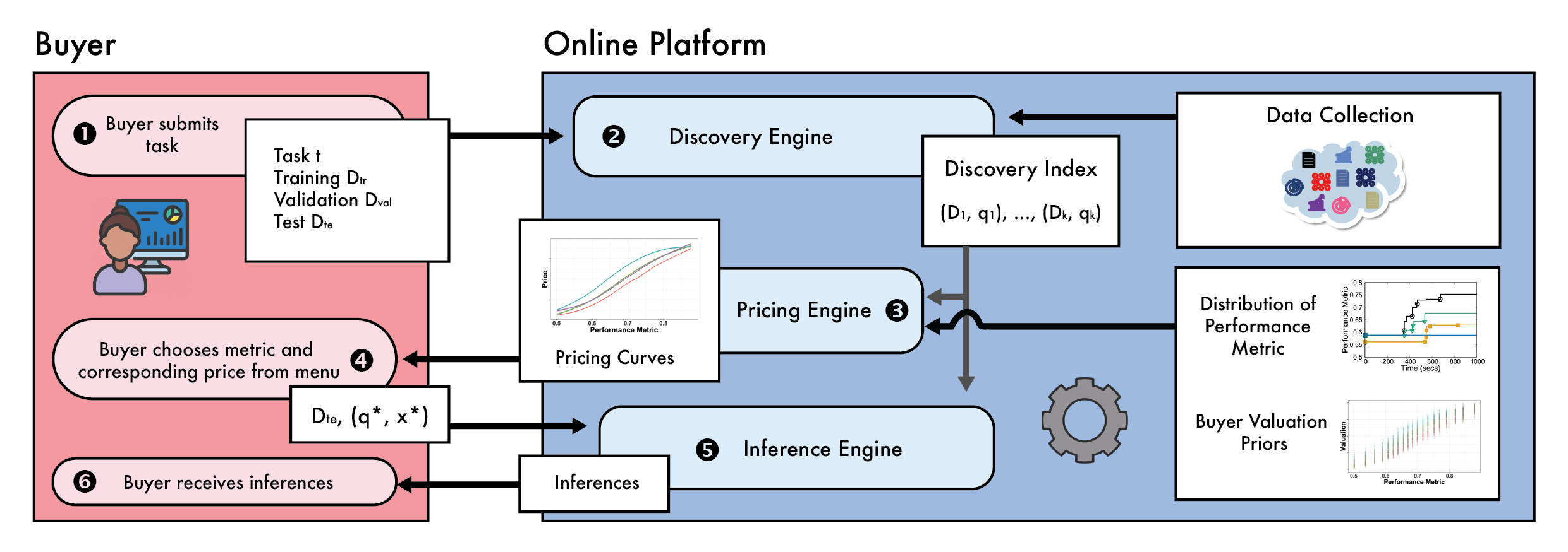
Figure 1: Overview of the market architecture. Circled numbers refer to the timing of events in the interaction protocol (Sec 3.2.3).

2 Discussions on Related Work

ML and Data Markets. Many ML markets have been proposed in previous work [2, 12, 56, 37, 55]. They have also considered selling the instrumental value of data, by building a model over all data in the market and selling different versions of the model to buyers with different preferences. Most of them assume all data in the market are relevant to the task, and thus do not consider the discovery problem. Yet, in a market with a large data collection, only a small subset may be relevant for any given task, hence our market’s emphasis on solving this challenging problem.  [36] does not assume all data in the market is useful, and studies how a buyer can interactively send queries to a market to obtain subsets of available data to improve an ML model at hand. It does not study the pricing problem. Much work in data markets concentrates on the question of privacy [52, 33, 60, 56, 37]; we take the same privacy model that today’s existing AutoML solutions use as a proxy towards a model that users find valuable, as these solutions already have a base of users. Lastly, today’s commercial online data marketplaces, such as Snowflake’s, AWS’s, sell raw data [54, 4]; we concentrate on selling the instrumental value of data, identifying relevant data by its impact on the buyers’ tasks, thus avoiding the main challenge of helping buyers decide how raw data helps their purpose.

Data Valuation. The line of work on data valuation [24, 31, 34, 51, 23, 59] is relevant to our data-centric ML market. Much work uses the notion of Data Shapley, which measures the value of a data point or a group of data points by how much they change the performance of a model. This is another measure of the instrumental value of data. From a buyer’s perspective, the market can combine all the data, train a model, and use Data Shapley to find the most valuable data points for the buyer’s task. Such an approach would be computationally prohibitive; this paper proposes a computationally feasible way to sell the instrumental value of data. From a data owner’s perspective, data valuation can be an important tool for revenue allocation, as suggested in  [59]. Additionally, as our market learns the instrumental value of datasets while searching, there is an opportunity to leverage this information to cheapen the valuation of datasets. In this case, the pricing mechanism proposed by our market could be complementary to existing work in data valuation.

Pricing Problem. The contract design literature [43, 28] studies the problem where a platform sets a contract of payments to maximize the expected revenue. Contract theory has played a significant role in economics [25, 53, 35], and there has been a growing interest in the computer science community regarding the problem of contract design driven by the increasing prevalence of contract-based markets in web-based applications [3, 9, 10, 22]. These markets have significant economic value, with data and computation playing a central role. In contrast to traditional contract design challenges, our design is on crafting contracts, specifically pricing curves in a data-centric ML market setting. Online pricing against strategic buyers is also widely studied in the economic literature [19, 11, 16, 45, 18]. Prior research primarily concentrated on analyzing various aspects of equilibria, with optimization efforts dedicated towards maximizing revenue for data owners. Our work takes a broader perspective by addressing the optimization of both buyer utility and the overall market welfare.

3 Data-Centric Machine Learning Market Architecture

We now present our design for a data-centric machine learning market (the market). On a high level, buyers bring their tasks to the market, and the market identifies data that improves the tasks’ performance and assigns a price to such improvement. We present the problem statement (Section 3.1, followed by the market architecture (Section 3.2).

3.1 Definitions and Problem Statement

Definition 3.1 (Performance Metric).

Given a model $C$ trained on dataset $D$, the performance metric, denoted by $m(C\leftarrow D)$, is the quality of the model over some test data $D_{te}$. For example, for a classifier, a performance metric may be an accuracy of 90%.

Definition 3.2 (Buyer).

A buyer has a machine learning task $t$, which is characterized by training data $D_{tr}$, validation data $D_{val}$, test data $D_{te}$, and the buyer’s choice of a measure of the performance metric. Buyers exhibit different types, leading to varying levels of value assigned to different performance metrics.

We assume the platform collects and uses buyers’ data, similar to existing AutoML platforms. While some buyers might express concerns about potential data leaks on the platform, many existing users of AutoML platforms do not share those same apprehensions. Therefore, we incorporate this perspective into our model as well.

Problem 1 (Pricing Problem).

When provided with a prior distribution $\mu$ regarding the types of buyers $\Theta=\{\theta_{1},\cdots,\theta_{n}\}$, and a model describing the evolution of performance metrics, the pricing problem involves assigning prices to each potential performance metric in order to maximize the expected revenue of the data market.

Definition 3.3 (Data Collection).

A data collection contains a set of datasets $\mathcal{D}=\{D_{1},\ldots,D_{n}\}$, where different datasets $D_{i},D_{j}$ may contain overlapping values. In this work, we assume each dataset $D_{i}$ is tabular, as is common in many enterprise scenarios.

Definition 3.4 (Join Path).

A join path $P$ is defined as an ordered list of datasets $P\equiv\{D_{1},\ldots,D_{t}\}$ such that datasets $D_{j}$ and $D_{j+1}$ join for all $j<t$ with each other forming a chain of join operations. We say the original dataset $D_{in}$ can be augmented using $t$ datasets.

Adding additional features using such database joins and searching across different ML models could help to improve the performance metric of a model. Thus, identifying profitable join paths is one way of doing feature engineering.

Problem 2 (Data and Model (DnM) Discovery).

Given a training dataset $D_{tr}$, a set of join paths $\mathbf{P}$ (where each join path translates to a different augmentation), a collection of ML models $\mathbf{M}$, identify a minimum set of augmentations $T\subseteq\mathbf{P}$ and an ML model $M\in\mathbf{M}$ such that $m(M\leftarrow(D_{tr}\Join T))$ is maximized.

Next, we present the architecture of the proposed data market.

3.2 Market Architecture and Interaction Protocol

Figure 1 presents the components of the market architecture. We first describe buyer’s interaction with the market and set their goals. Then, we describe the platform’s tasks.

3.2.1 The Buyer Perspective

Task Specification. The buyer specifies the task details: training, validation, and testing data, along with a measure of the performance metric. The buyer submits this to the market and starts paying for search costs: the longer the market works on the task, the more they pay. This is the same mechanism used by today’s AutoML platforms and, more generally, many other cloud services.

Price-Metric Dashboard. The market offers a menu of ML models, each achieving a different performance metric, and each associated with a price. Buyers who are satisfied with the current options choose one and stop the search. Alternatively, buyers can continue paying for search to populate the menu with additional options and prices. A reasonable assumption about the buyers is that they want a positive net utility, defined as the disparity between their payoffs and the costs associated with their actions, such as the contrast between value and payment in auctions or revenue and cost in markets [42, 30, 7].

Data Label Collection. Once the buyer chooses a model from the menu and makes a payment, the market uses the user’s model choice to calculate inferences for the test dataset, and returns the inferences to the buyer.

Note that in our design, the market does both training and inference. For this reason, we design the market such that buyers need to cover these costs. The payment of any buyer consists of two components 1) the search cost of doing data and model search, and 2) payment per inference, calculated from the buyer’s chosen data-augmented ML model.

Definition 3.5 (Buyer Utility).

The buyer $\theta$’s utility depends on three terms: $u^{\theta}(q,x,c)=v^{\theta}(q)-x(q)-c$, where $v^{\theta}(q)$ denotes the buyer’s value of performance metric $q$, $x(q)$ denotes the price charged for this performance metric, and $c$ denotes the search cost of the buyer.

3.2.2 The Platform Perspective

At time 0, before buyers arrive, we endow the platform with the following information:

Data Collection. A collection of datasets, $\mathcal{D}=\{D_{1},\ldots,D_{n}\}$, that are used by the market to discover augmentations by joining with the initial data $D_{tr}$. In this paper, we assume the platform fully owns these datasets, e.g., a large company seeking to monetize access to their data. In a more general setting, these datasets could come from different owners.

Buyer’s valuation prior. A prior distribution $\mu\in\Delta^{n}=\{y:\sum_{i\in[n]}y_{i}=1\}$ over the buyer types $\Theta=\{\theta_{1},\cdots,\theta_{n}\}$, where $\mu_{i}$ denotes the probability of buyer type $\theta_{i}$. The assumption of a prior in market design research serves as a foundational element that helps capture the model and the inherent uncertainty and information asymmetry present in real-world scenarios [43, 48, 14]. In market science, such a buyer-type prior distribution can typically be learned from market surveys [41, 43].

Performance Metrics Distribution. Given a task and data collection, we can obtain the sequence of performance metrics the market produces for the task. We assume the market has a collection of performance metric sequences for a sample of possible tasks.

3.2.3 Interaction Protocol

When a buyer arrives in the market and submits a task, the timing is as follows:

\raisebox{-0.9pt}{1}⃝ Task Submission. A buyer submits a task to the market, which consists of a specification of training data $D_{tr}$, test data $D_{te}$, validation data $D_{de}$, and a measure of the performance metric. The buyer can choose cross-validation on the training data instead of using test data for evaluation. The training and test sets must have the desired prediction (independent, target) variables, while the validation set need not have the independent variables.

\raisebox{-0.9pt}{2}⃝ Search. The discovery engine takes the buyer’s task and searches for data augmentations, $D=(D_{tr},D_{val},D_{te})$ using the discovery index. The discovery engine incrementally produces a list of ($D_{i}$, $q_{i}$) pairs, where $D_{i}$ denotes an augmentation, and $q_{i}$ denotes the associated metric value computed using this augmentation, on the test data or cross-validation.

\raisebox{-0.9pt}{3}⃝ Offer Price Curve. From buyer’s choice of the metric and the calculated $q_{i}$, the pricing engine looks up the price $x_{i}$ from the price curve that corresponds to buyer’s chosen metric type. It then sends the list of ($q_{i}$, $x_{i}$) pairs to the buyer.

\raisebox{-0.9pt}{4}⃝ \raisebox{-0.9pt}{5}⃝ \raisebox{-0.9pt}{6}⃝ Offer Selection, Payment, and Service. Buyer chooses the desired performance metric $q_{i}$ from the list, and makes a payment for the inferences they want to obtain. Based on the choice of $q_{i}$, and hence the corresponding $D_{i}$, the inference engine makes predictions on the test set, and sends the predictions to the buyers. Note that buyers only get access to the predictions, not the raw dataset. This eliminates the possibility of buyers distributing the raw dataset for free after obtaining it, mitigating some of the privacy concerns when the datasets are contributed by various data owners.

3.3 Summary of Contributions

From the buyer’s perspective (see Def. 3.5), an ideal solution is a market that spends no time searching for a model (to reduce search costs) that yields the highest performance metric at the lowest cost. The main contributions of our work are geared towards this ideal.

Discovery Engine. The discovery engine identifies datasets to augment $D_{tr}$ and generates a suite of options with different performance metrics, catering to different buyers’ preferences. The desiderata for the discovery engine is that: i) it must be efficient, ii) support anytime search, and iii) identify the best ML model. The first two requirements are needed so that the buyer can search only for as long as they are willing to pay. The third is needed so that the engine guarantees to do its best in finding the best model (Section 4).

Pricing Engine. The pricing engine models different market participants, and computes optimal market mechanisms. The desired qualities for the pricing engine are that: i) has a transparent training process to reduce buyer risk, and ii) computes the market mechanism to maximize the revenue. The first requirement gives the buyer flexibility such that the buyer can choose when to stop and whether to purchase. The second is needed so that it supports the sustainability and growth of the market. (Section 5).

4 Discovery Engine: Efficient Data and Model Discovery

In this section, we study the problem of effectively discovering data and ML models for the end-user’s downstream application.

A trivial approach to solve Problem 2 is to consider every combination of sets of augmentations and ML models to return the best combination. On one hand, this approach would give the optimal solution, but it is intractable to train $O(2^{|\mathbf{P}|}|\mathbf{M}|)$ ML models where $|\mathbf{P}|$ is often in the order of millions. Longer runtime translates into higher search costs that reduce the number of buyers who benefit from the market. Although the general problem is intractable, prior data discovery methods have studied ways to prune the search space in settings where the downstream model is fixed. Specifically, Metam [21] leverages properties of the data (datasets that are similar often yield similar performance metrics on ML models) and the search problem to prune irrelevant augmentations and prioritizes them in the order of their likelihood to be useful for the end user.

Intuitively, this approach ranks the different augmentations and trains an ML model to test the top-ranked augmentation. The metric of the trained ML model is used as feedback to re-rank other augmentations and the process is continued. This approach has been shown to converge in $O(\log{\mathbf{P}})$ such rounds of testing the top-ranked augmentation. Naively applying such techniques would require us to train each ML model whenever the top-candidate augmentation is tested. Therefore, it would require $O(|\mathbf{M}|\times\log|\mathbf{P}|)$ model trainings. Even though this approach seems theoretically feasible, it is time-consuming (and thus expensive) to train thousands of ML models. In this work, we present an efficient mechanism to choose the best dataset and model simultaneously. Specifically, we model each ML model as an arm and simulate a bandit-based learning problem to choose the best model. Note that our problem is similar to pure exploration framework, as the goal is to choose the best model and stop exploration after that.

Algorithm 1 Model Discovery Algorithm

Input: Training Data $D_{tr},D_{val}$, List of Models $\mathbf{M}$, Augmentations $\mathbf{P}$
Output: ML Model $M$

1:  Initialize the solution set of augmentations $\mathbf{T}\leftarrow\phi$

2:  Initialize $w(M)=1,\forall M\in\mathbf{M}$, $\gamma=0.1$

3:  while $i\leq\textsc{StoppingCriterion}$ do

4:     Choose a candidate augmentation $T_{i}\subseteq\mathbf{P}$ using [21]

5:     Set $\texttt{Pr}(M)=(1-\gamma)\frac{w(M)}{\sum_{M\in\mathbf{M}}w(M)}+\frac{\gamma}{|\mathbf{M}|}$

6:     $M_{i}\leftarrow$Sample a model $M$ according to the probability distribution Pr.

7:     Update $w(M_{i})=w(M_{i})e^{\gamma\widehat{r}(M)}/|\mathbf{M}|$, where $\widehat{r}(M)=m(M_{i}\leftarrow(D_{in}\Join T_{i}))*1.0/Pr(M_{i})$

8:  end while

9:  $\widehat{T}\leftarrow$ Best augmentation set according to [21]

10:  Return $arg\mathop{max}_{M}m(M\leftarrow D_{in},\widehat{T})$

Algorithm 1 presents the pseudocode of our proposed mechanism. It uses Exp3 (Exponential-weight algorithm for Exploration and Exploitation, [5]) to choose the best arm. We initialize each model with an equal weight of $1$. In each iteration, we estimate the probability of choosing a model as $\texttt{Pr}(M)=(1-\gamma)\frac{w(M)}{\sum_{M\in\mathbf{M}}w(M)}+\frac{\gamma}{|\mathbf{M}|}$, where $\gamma$ is the exploration parameter. Setting $\gamma=1$ is equivalent to choosing a random model each time. A model is chosen based on this probability distribution and trained on the initial dataset augmented with augmentation $T_{i}$. The metric $m$ evaluated on the trained model is used as the reward to update $w(M)$. The main advantages of the Exp3 algorithm are that the adversarial bandit-based formulation helps to model the changing input dataset in each iteration and it has shown superior empirical performance in practical scenarios [8]. The StoppingCriterion implements the anytime property, letting buyers stop searching whenever they want. Algorithm 1 trains a single ML model in each iteration as opposed to $|\mathbf{M}|$ trainings by prior techniques. Further, we extend the result from [21] to show that our algorithm identifies a constant approximation of the optimal solution by training $O(\log|\mathbf{P}|)$ ML models under practical settings.

Theorem 4.1.

Given an initial dataset $D_{in}$, set of augmentations $\mathbf{P}$ and ML models $\mathbf{M}$, our algorithm identifies a solution $T\subseteq\mathbf{P}$ and $\widehat{M}\in\mathbf{M}$ in $O(\log(|\mathbf{P}|)+|\mathbf{M}|)$ ML model trainings such that

$$m(\widehat{M}\leftarrow D_{in}\Join T)\geq m(M^{*}\leftarrow D_{in}\Join T^{*})\times\left(\frac{1}{\alpha}(1-e^{-\alpha\eta})-k\epsilon\right)$$

where $T^{*},M^{*}$ denote the optimal solution and $k,\epsilon$ are constants, $\alpha$ and $\eta$ are curvature and submodularity ratio of $m$.

Our approach is the first to do data and model search effectively and efficiently. The use of the Exp3 algorithm to interleave between the two different searches: model and dataset, helps to reduce the computational complexity of the naive approach without loss in quality. We have evaluated the advantages of our choice empirically in Section 5. Our data and model discovery approach relies on the mechanisms discussed in [21] to choose the best candidate augmentation in each iteration. This approach follows the following steps. i) candidate generation and likelihood estimation; ii) adaptive querying strategy. The first component identifies the candidate augmentations and computes a feature vector of their properties. The second component ranks the different candidate augmentations and iteratively chooses the best augmentation. This augmentation is given to our model discovery algorithm (line 4 in Algorithm 1).

Candidate Generation and likelihood estimation. This component first identifies features that can augment $D_{in}$ using database joins. Each candidate feature is processed to compute its vector of data profiles. These profiles are used to cluster candidate augmentations based on their similarity. Intuitively, augmentations in the same cluster are expected to have a similar model performance and therefore, the discovery approach chooses representatives from each cluster for the subsequent stages. The profile-based feature vector for each augmentation is also used to calculate a likelihood score, denoting how likely an augmentation would improve model performance.

Adaptive Querying strategy. This component uses the identified clusters and their likelihood scores to choose an augmentation for training an ML model. This component interleaves between two complementary strategies (sequential and group querying), which are shown to have varied advantages. The sequential approach estimates the quality of each candidate augmentation and greedily chooses the best option. The group querying strategy considers augmentation subsets of different sizes to train the ML model. Group selection internally relies on the Thompson sampling method to sample an augmentation for each iteration.

This result indicates that the discovery approach is highly efficient in identifying useful augmentations and is capable of generating a solution at any point of time, allowing the buyer to stop whenever needed based on their measure of utility $u^{\theta}(q,x,c)$. To prove the approximation ratio of our discovery algorithm, we assume that any augmentation $T$ that helps to improve $M^{*}\leftarrow D\Join T$’s performance metric the most remains consistent across different ML models. The formal proof can be found in Appendix A.

5 The Pricing Engine: Finding Metric-Price Menus

The evolution of model metric and discovery cost. To design the market, we need to model the output of the discovery engine, i.e., the sequence of performance metrics it produces. The market reveals to buyers the current model metric at pre-specified time points/periods $1,2,\cdots,T$ (e.g., every $5$ minutes). Let $q_{t}\in Q$ denote the present model performance metric at time period $t$. We assume $q_{t}$ has finite resolution and is drawn from a discrete set $Q$ of all possible (rounded) metrics. Notably, $q_{t+1}$ may be smaller than $q_{t}$ since it is the latest discovered model metric, which may become worse due to searching over worse data sets during the data discovery process. Revealing the latest model metric, while not the best metric so far which will be monotone, is a tailored design choice since we would like to provide users with a variety of choices because some users may prefer a lower-quality data set at a lower price.

Since most ML algorithms are based on gradient descent [27, 58]; given its current performance determined by current parameters, its future performance is often independent of previous parameters. This means the model’s performance metric can be well-approximated by a Markov chain. This characteristic is particularly prominent in optimization algorithms like gradient descent, where updates are driven by the immediate surroundings of current parameter values [50]. We thus denote the accurate evaluation of the data discovery procedure as a Markov chain $\langle Q,T,\{\bm{P}_{t}\}_{t\in[T]}\rangle$, in which $\bm{P}_{t}(q_{t}|q_{t-1})$ is the transition probability from previous state $q_{t-1}$ to the current state $q_{t}$. It is important to allow $\bm{P}_{t}$ to be time-dependent because the probability of transitioning from metric $q$ to $q^{\prime}$ typically differs a lot at different times (e.g., the later, the less likely to have a big increase).

In contrast to the uncertainty of model metric evolution, we assume the data discovery cost is a stable constant $c$ for each unit of time since this cost is often determined by the computation time, and thus each unit of computing time experiences a similar cost.

Modeling the market and buyer demand. The market is divided into different segments for different categories of ML tasks (e.g., financial prediction, agriculture product prediction, location-based marketing, etc.). Each segment is relatively independent with a different data pool and buyer demand, and thus will be treated separately. The buyers’ demand and preferences within a segment are expected to have less variance. Following standard economic assumptions [38, 41, 43], there is a population of buyers who are interested in this particular segment (i.e., agriculture product prediction). Each buyer is modeled by a private type $\theta\in\Theta$. Each $\theta$ determines a vector $v^{\theta}(\cdot)\in\mathbb{R}_{+}^{Q}$, in which $v^{\theta}(q)$ describes her values for model metric $q\in Q$. While the buyer knows his type $\theta$, the marketplace only knows a prior distribution $\mu$ about the buyer population, which can be viewed as the platform’s estimation of the market’s distributional interests in this segment.

5.1 Designing Pricing Mechanisms to Bridge the Discovery Engine and Market

Interaction protocol. We now describe our designed mechanism for pricing data-augmented ML models. Our mechanism bridges the data discovery engine (which supplies model performance metrics in real-time) and the market (which supplies a population of potentially interested buyers). Specifically, our mechanism is a simple price curve (PC) $x\in\mathbb{R}_{+}^{Q}$, which prescribes a price $x(q)$ for each possible performance metric $q\in Q$. Notably, this PC $x$ will be posted in advance so that it is public information to every potential buyer. During the data discovery process, the user sees all available performance metrics thus far, can choose to stop at any time, and moreover, can choose to purchase the model or leave the market.

Payment structure. The payment of any buyer consists of two components: (1) the data discovery cost $c\tau$ in which $\tau\ in[T]$ is the user’s stopping time and $c$ is the true computation cost per unit of time; (2) payment $x(q)$ per inference if the buyer chooses to purchase a data-augmented ML model with performance metric $q$ for inference. The payment of data discovery cost is mandatory, in order to sustain and compensate the system’s operation. However, we expect this cost to be very low and can be viewed as a form of entry fee. The payment of $x(q)$ per inference is voluntary and represents what our platform truly sells.

5.2 Analysis of Buyer Behavior and Optimization of Pricing Mechanism

Buyer’s behavior as optimal stopping. Since the buyer knows the price and search cost before starting data and model discovery, she faces an optimal stopping problem when participating in our market. More precisely, the buyer’s search for model performance metric is precisely a Pandora’s Box problem, a widely studied online optimization problem to balance the cost and benefit of search [57, 6, 17]. Here, an agent is presented with various alternatives modeled by a set of boxes $B=\{b_{1},\cdots,b_{n}\}$, where each box $b_{i}$ needs cost $c_{i}$ to be opened, and has a random payoff $v_{i}$ whose distribution is known. The agent’s goal is to find a strategy that adaptively decides whether to stop or continue the search after opening each box. Similarly, in our problem, the buyer also needs to make the decision to continue or stop at every time step $t\in[T]$. A major difference between our problem and Pandora’s box problem is that they assume all boxes’ payoff distributions are independent, while in our problem the buyer’s random payoff of the next time step (i.e., box) depends on the state of the current time step. This dependence is modeled through the Markov chain $\{\bm{P}_{t}\}_{t\in[T]}$. See Figure 2 for an illustration.

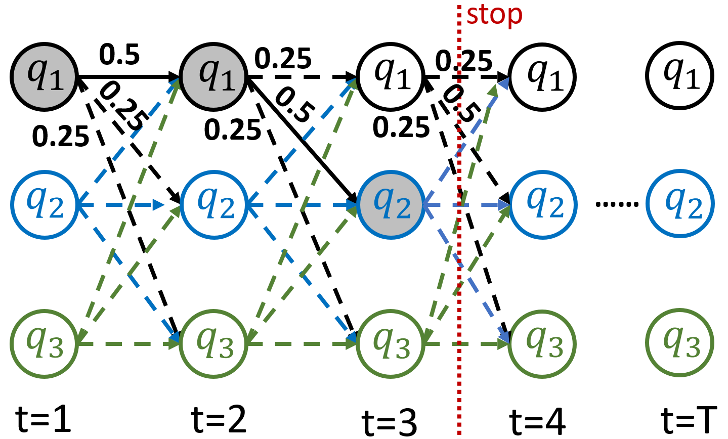
Figure 2: A Markov chain model where the buyer makes a decision to continue or stop at every node.

Let us consider the case where the buyer faces a price curve $x\in\mathbb{R}^{Q}_{+}$. At time step $t$, suppose the maximal performance metric the buyer has seen is denoted as $q=\mathop{max}_{t^{\prime}=1}^{t}q_{t^{\prime}}$, the realized performance matric at time step $t$ is denoted as $q_{t}$, we denote $\tau(q,q_{t},t)$ as the (random) stopping time conditioned on the events $\tau\geq t$. Given any $\tau$, we can define its corresponding expected future reward starting in state $(q,q_{t},t)$ for the buyer of type $\theta$ as

$$\begin{split}\phi^{\tau}(q,q_{t},t)=\mathbb{E}\Big{[}v^{\theta}\Big{(}\mathop{max}\big{(}q,\mathop{max}_{t^{\prime}=t+1}^{\tau(q,q_{t},t)}Q_{t^{\prime}}\big{)}\Big{)}-x\Big{(}\mathop{max}\big{(}q,\mathop{max}_{t^{\prime}=t+1}^{\tau(q,q_{t},t)}Q_{t^{\prime}}\big{)}\Big{)}\Big{]}-\sum_{t^{\prime}=t+1}^{\tau(q,q_{t},t)}c.\end{split}$$

where $Q_{t}$ denotes the random variable and $\mathop{max}\big{(}q,\mathop{max}_{t^{\prime}=t+1}^{\tau(q,q_{t},t)}Q_{t^{\prime}}\big{)}$ denotes the best metric the buyer can find until the stopping time $\tau(q,q_{t},t)$. We define $\Phi(q,q_{t},t)=\mathop{max}_{\tau}\phi^{\tau}(q,q_{t},t)$ that represents the expected optimal future reward the buyer can achieve in state $(q,q_{t},t)$ under the optimal policy $\tau^{*}=\arg\mathop{max}_{\tau}\phi^{\tau}(q,q_{t},t)$. Thus, the buyer’s goal is to compute a $\tau^{*}$ that maximizes $\phi^{\tau}(q_{0},q_{0},1)$, i.e., the buyer’s expected future reward starting at the initial metric $q_{0}$ at the starting time $t=1$. Next, we show that the buyer can efficiently compute the optimal policy via carefully designed dynamic programming.

Proposition 5.1.

The optimal buyer policy can be computed efficiently via dynamic programming in $O(Q^{2}T)$ time.

Our dynamic programming algorithm constructs one DP table $\Phi$ with shape $Q\times Q\times T$. Each entry $\Phi(q_{1},q_{2},t)$ in the table records the buyer’s optimal expected future reward the buyer can achieve at state $(q_{1},q_{2},t)$, i.e., at time step $t$, the maximal performance metric the buyer has seen is $q_{1}$, while the realized performance metric at time step $t$ is $q_{2}$. Since the underlying process is a known MDP, the buyer’s future expectations depend only on the current performance metric $q_{2}$. Using this table, we can then calculate the buyer’s optimal stopping policy $\tau^{*}$ by comparing the difference between the buyer’s utility if they stop right now and the expected future utility of continuing.

We defer the proof to Appendix B, and only note here that the core to the proof is to identify a recursive relation between current reward and expected future reward, summarized as follows:

$$\Phi(q_{1},q_{2},t)=\mathop{max}\Big{(}v^{\theta}(q_{1})-x(q_{1}),\mathbb{E}_{\bm{P}(q|q_{2})}\big{[}\Phi(\mathop{max}(q_{1},q),q,t+1)\big{]}-c\Big{)}.$$

Finding the optimal pricing curve from empirical data. Next, we show how to approximately compute the optimal pricing curve from the empirical data. To do so, we formulate a mixed integer linear program to approximately compute the optimal pricing curve with input from both the market and discovery engine.

Given a common prior distribution $\mu$ over the buyer population and sampled metric trajectories from the empirical data discovery process. Specifically, we sample a set of metric trajectories $S=\{s_{1},\cdots,s_{m}\}$ where $s_{i},i\in[m]$ represents a sequence of model metrics discovered in a prefixed period (i.e., $s_{i}=[q_{1},\cdots,q_{T}]$). The following theorem guarantees the computation of a solution from a Mixed Integer Linear Programming (MILP) that provably approximates the optimal pricing curve under mild assumptions. The MILP can be solved efficiently by industry-standard solvers such as Gurobi [26] or Cplex [15].

Theorem 5.2.

Let $m=|\widehat{S}|$ be the number of samples in $\widehat{S}$ and suppose the discovery cost $c$ is negligible compared to the buyer’s value. Then with probability at least $1-2\delta$, the following MILP with variable $x$ computes a pricing curve that is an additively $\epsilon$-approximation to the optimal curve where $\delta=\exp(\frac{-2m\epsilon^{2}}{b^{2}})$, $b$ is the maximum valuation from any buyer, and $\epsilon>0$ is the error term.

$$\begin{split}\mathop{max}\quad&\sum_{\theta}\mu(\theta)\sum_{s\in S}\frac{1}{m}\sum_{q^{s}\in s}y(\theta,s,q^{s})\\ \text{s.t.}\quad&0\leq a_{\theta,s}-\big{[}v^{\theta}(q^{s})-x(q^{s})\big{]}\leq M\big{(}1-z(\theta,s,q^{s})\big{)},\,\,\forall\theta,s,q^{s}\\ &\textstyle\sum_{q^{s}}z(\theta,s,q^{s})=1,\,\,\forall\theta,s,\\ &y(\theta,s,q^{s})\leq x(q^{s});\quad y(\theta,s,q^{s})\leq Mz(\theta,s,q^{s}),\,\,\forall\theta,s,q^{s}\\ &y(\theta,s,q^{s})\geq x(q^{s})-\big{(}1-z(\theta,s,q^{s})\big{)}M,\,\,\forall\theta,s,q^{s}\\ &\bm{x}\geq 0;\quad\bm{z}\in\{0,1\};\quad\bm{y}\geq 0.\end{split}$$ (1)

We briefly discuss the core assumption of the above theorem, i.e., the assumption that the data discovery cost $c\tau$ is negligible compared to the model price and buyer valuations. Note that, the discovery cost $c\tau$ in our pricing scheme is different from the payment in the existing AutoML market which charges buyers $\alpha\tau$ for running on their cloud for $\tau$ time. The $\alpha$ in their pricing model is the price per unit of computation, whereas $c$ in our scheme is the true computation cost (electricity and server amortization cost). Generally, $\alpha>>c$.

6 Evaluation

In this section, we evaluate the feasibility of implementing the proposed market in practice. Specifically, we study the effectiveness of our model discovery engine proposed in Section 4 and our pricing engine discussed in Section 5.

Experimental Setup. We consider buyers who want to train a highly accurate ML model by searching over the data collection and ML models. We implement a market with a search space of $69K$ datasets (with $\approx 30$M columns and $3$B rows) from the NYC open data repository. The market searches over these datasets to identify the best combination of augmentations and models (random forest, XGBoost, neural network, etc.) that help improve buyers’ input tasks.

6.1 RQ1: How does the discovery engine perform?

We first present results for two different supervised ML tasks (i) Classification: We considered a school counselor as a buyer who presents an initial dataset about different schools in NYC to predict the performance of those schools on a standardized test. The goal is to maximize the F-score of the trained model. The initial dataset has 2000 records, and 6 features. (ii) Regression: We considered a buyer who uploads taxi dataset to predict the number of collisions using information about their daily trips. The goal is to minimize the relative error in the prediction outcome. The initial dataset has 400 records, and 4 features.

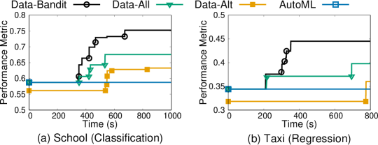
Figure 3: Comparing discovery techniques on School/Taxi Task

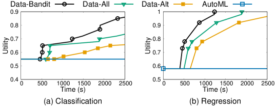
Figure 4: Comparing discovery techniques on 1K Input Tasks

We consider three competitive baselines to compare the effectiveness of our discovery algorithm. (i) Data-All uses [21] to search for the best augmentations and trains all ML models in each iteration to choose the best model. (ii) Data-Alt fixes a high-efficiency low-cost ML model (random forest classifier in this case) to test the chosen augmentation in each round and then trains an AutoML model (using the TPOT library) on the best augmentation every minute. (iii) AutoML approach does not search over datasets, only models using TPOT. We represent our approach as Data-Bandit.

Figure 3 compares the evaluation metric of the trained model for Data-Bandit with other baselines. The x-axis represents search time in seconds, and the y-axis represents utility. The initial performance metric denotes the accuracy of the ML model without any additional data. The metric remains constant for $6$ minutes for schools and $3$ minutes for the taxi dataset, as our discovery approach spends the initial few minutes searching for potential augmentations and ranks them. We observe that the model trained by our discovery approach has an F-score of more than $0.70$ in less than $7$ minutes for the school’s task, as opposed to other techniques that require more than $15$ minutes for a similar F-score. We observe similar differences for the taxi dataset. We manually inspected the results and identified some interesting augmentations e.g. crime information, income of people staying in a neighborhood, presence of grocery stores, etc. After augmentation, the school and taxi dataset contain 9 and 8 additional features, respectively.

Zooming away from the two tasks above, Figure 4 reports the average results on a sample of 1000 different tasks (classification and regression for different input datasets). All initial datasets contain more than 500 records. We observe that the bandit-based approach used by our discovery engine outperforms all baselines consistently across the considered tasks by achieving a higher utility for the buyers in a shorter amount of time. For classification tasks, the average utility found by our platform is higher than 0.85, whereas the second-highest benchmark is just above 0.7. AutoML does not search for data, and its average utility for classification is around 0.55. For regression tasks, our platform also performs better: fix any point on the x-axis (search time), and our platform achieves higher utility than all baselines. For most tasks, the number of augmentations identified is less than 10. Notice that a higher running time of the discovery algorithm translates to higher waiting times and computing costs for the buyer. Although the additional computation cost incurred by higher running time is small for buyers with high valuations, it can become significant for buyers with low valuations of tasks. This experiment shows that our approach can identify the best model consistently across different tasks, and is effective in generating a suite of options for the buyer to choose from based on their budget and performance metric requirements.

6.2 RQ2: How do different pricing schemes perform?

In this evaluation, we study how much profit our pricing algorithms generate, as a fraction of the total possible welfare, for both in sample (IS) and out of sample (OOS) performance metric trajectories. We train our pricing algorithms on the sample, produce pricing curves, and evaluate how much profit we earn using these pricing curves.

We generate the buyer valuations for both IS and OOS using the same random process and draw a new independent sample every time. In IS training, all performance metrics are available to the buyer, while in OOS, a random subset of performance metrics is drawn each time from real performance metrics that buyers might encounter using real data. We evaluate the performance metrics for different tasks to identify a plausible set of performance metrics and limit the buyer to only choosing from a randomly sampled limited pool of performance metrics OOS. This places a significant limitation on our pricing algorithm while OOS, which creates a good test of robustness.

In addition to the nearly optimal pricing curve solved by our MILP (1), we present three pricing baselines in increasing order of complexity and flexibility to fit the sample data, which help demonstrate how bias and variance interact in the context of pricing.

Independent pricing scheme.

Given a prior distribution $\mu\in\Delta^{|\Theta|}$ over the buyer types, where each buyer type $\theta$ has a value $v_{q}[\theta]$ for performance metric $q$, we can consider the valuation $V_{q}$ as a random variable with $\mathbb{P}(V_{q}=v_{q}[\theta])=\mu(\theta)$. The independent pricing scheme assumes that $V_{q}$ is independent of $V_{q^{\prime}}$ for any $q\neq q^{\prime}$, and computes the price for each performance metric that maximizes the expected payment with respect to the prior distribution $\mu$: $x(q)=\arg\mathop{max}_{x}\mathbb{E}_{\theta}[x\mathbbm{1}_{v_{q}[\theta]\geq x}],$ where $\mathbbm{1}(\cdot)$ is the indicator function. Since $V_{q}$ is discrete, this scheme will always lead to a selection of $x(q)$ such that $x(q)=v_{q}[\theta_{q}]$ for some optimal $\theta_{q}$.

Shift pricing scheme.

The shift pricing shifts the independent pricing scheme up or down by some discrete shift parameter $k\in\{-|\Theta|,-|\Theta|-1,...,0,...,|\Theta|-1,|\Theta|\}$. Specifically, let $\theta_{q}^{0}$ be the $\theta$ chosen by the independent pricing scheme. Let $\theta_{q}^{k}$ be $\theta$ such that $v_{q}[\theta_{q}^{k}]$ is $k$-ranks higher or lower than $v_{q}[\theta_{q}^{0}]$ if we sort $\{v_{q}[\theta_{q}]|\theta\in\Theta\}$ from smallest to largest. Then the shift-$k$ pricing scheme sets the price $x(q)=v_{q}[\theta_{q}^{k}].$

The optimal linear pricing scheme can be found by a grid search for the optimal shift parameter $k^{*}$. Intuitively, the shift pricing scheme ‘shifts’ the independent pricing scheme up or down, with increments corresponding to the differences in valuations between buyers. Hence, shift pricing always performs better than independent pricing on sample data $\widehat{S}$.

Jiggle pricing scheme

The jiggle pricing algorithm takes an initial selection of $\theta_{q}$ values and tests out small changes to them to see if it improves the pricing scheme. Specifically, at each step, Jiggle tests out two possible modifications to $\theta_{q}$: (1) find a $q$ that has a high probability of being chosen and shift the price up to $x(q)=v_{q}[\theta_{q}^{1}]$ so that we charge more for popular performance metrics (2) find a $q$ that has a low probability of being chosen and shift the price down to $x(q)=v(q)[\theta_{q}^{-1}]$ so that we charge less for undesired performance metrics. Jiggle then continues to make such modifications on previous modifications that were successful, similar to the tree search. In our experiments, we set the maximum number of tested modifications to $\mathcal{O}(|\Theta||Q|)$, and the initial $\theta_{q}$ to be the $\theta_{q}^{k^{*}}$, the optimal solution for the shift pricing scheme. Hence, jiggle pricing always performs better than shift pricing on the sample data $\widehat{S}$.

Furthermore, we also included the optimal pricing scheme for OOS if all performance metrics were available to the buyer.

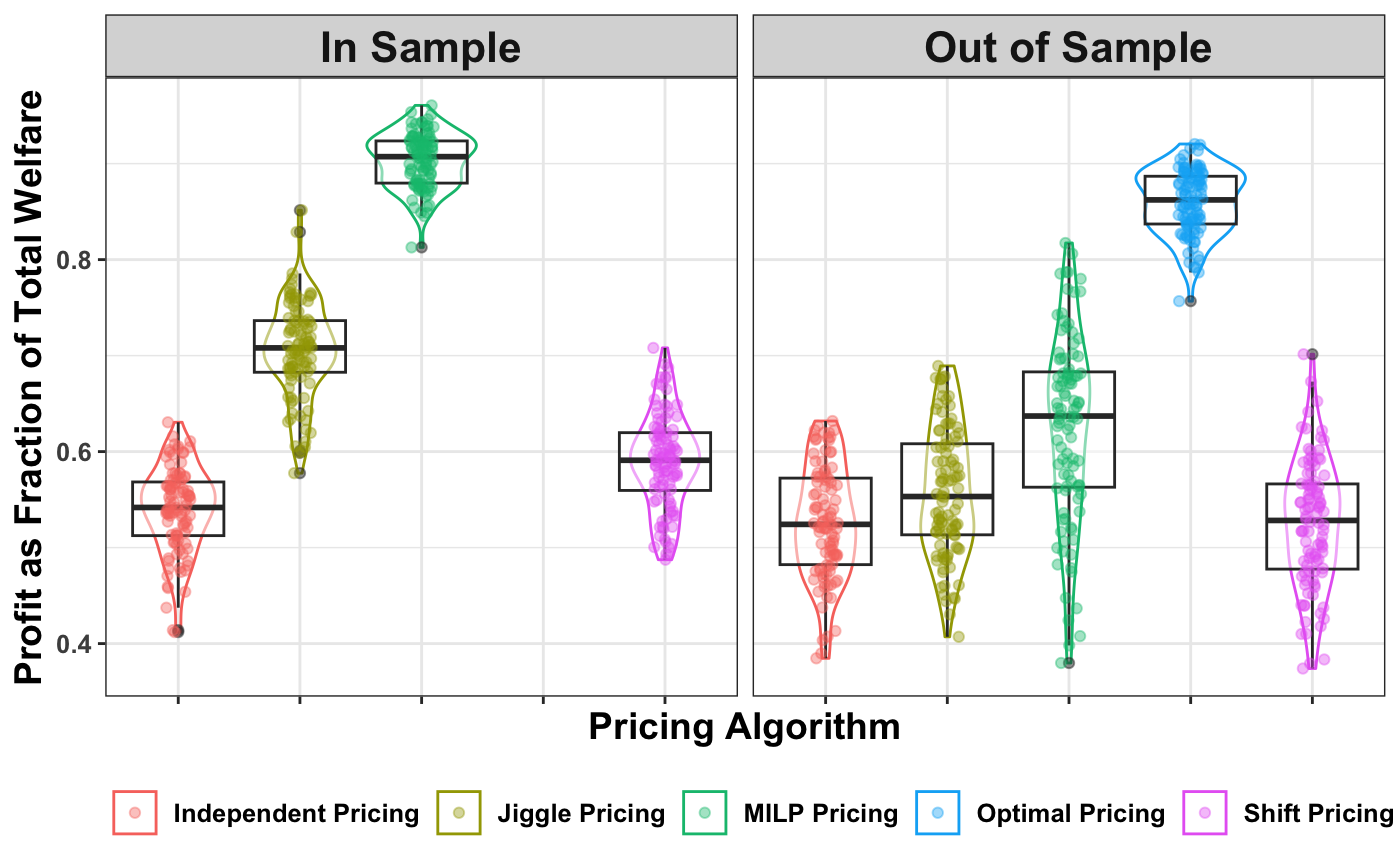
Figure 5: Profit Benchmark for School Data

Results

Figure 5 displays the performance of our algorithms in the IS and OOS setting, respectively . In both figures, the y-axis represents the normalized, expected profit as a fraction of the total welfare (ie. how much total surplus the buyers can get if all prices are set to $0$). The total welfare represents an upper bound on how well any mechanism can do. The higher a pricing scheme is, the more profit it is able to capture and the better it is. In the IS setting, the MILP outperforms our other algorithms, capturing around 85% of the total welfare, whereas all others capture less than 80%. In the adverse, OOS setting, MILP also outperforms the other baselines, only trailing the optimal pricing scheme. It is still able to capture a majority of the welfare.

7 Conclusion

In this paper, we study novel techniques to address core challenges in designing a data-centric online market for machine learning. By automating data and model discovery and implementing a novel pricing mechanism for data-augmented ML models, our market offers higher quality models for ML users compared to existing platforms, generates high revenue to compensate participants, all while being API-compatible and thus practical to use. Recognizing that designing a fully-functional, end-to-end online ML market still requires solving important challenges, we see this work as a step towards the bigger vision of building online markets for machine learning.

Acknowledgment.

This work is supported in part by an NSF Award CCF-2303372 and an Army Research Office Award W911NF-23-1-0030.

Appendix A Details on the Data and Model Discovery Algorithm

Theorem A.1.

Given an initial dataset $D_{in}$, set of augmentations $\mathbf{P}$ and ML models $\mathbf{M}$, our algorithm identifies a solution $T\subseteq\mathbf{P}$ and $\widehat{M}\in\mathbf{M}$ in $O(\log(|\mathbf{P}|)+|\mathbf{M}|)$ ML model trainings such that

$$m(\widehat{M}\leftarrow D_{in}\Join T)\geq m(M^{*}\leftarrow D_{in}\Join T^{*})\times\left(\frac{1}{\alpha}(1-e^{-\alpha\eta})-k\epsilon\right)$$

where $T^{*},M^{*}$ denote the optimal solution and $k,\epsilon$ are constants, $\alpha$ and $\eta$ are curvature and submodularity ratio of $m$.

Proof.

Using the result from [21], the optimal solution after clustering the candidate augmentations is $(1-k\epsilon)$ an approximation of the overall optimal solution. Further, the sequential querying strategy chooses the best augmentation in each iteration (this holds for any model because the best augmentation according to $M^{*}$ is also the best according to any other model $M$). Combining these results, we get the following [21].

$$m(M^{*}\leftarrow D_{in}\Join T)\geq m(M^{*}\leftarrow D_{in}\Join T^{*})\times\left(\frac{1}{\alpha}(1-e^{-\alpha\eta})-k\epsilon\right)$$ (2)

As a last step, Algorithm 1 chooses the best ML model for the returned augmentation $T$, implying $m(\widehat{M}\leftarrow D_{in}\Join T)\geq m(M^{*}\leftarrow D_{in}\Join T)$. Combining this with Equation 2 results, we get the desired result. ∎

Appendix B Omitted Proofs from Section 5

Proposition B.1.

The optimal buyer policy can be computed efficiently via dynamic programming in $O(Q^{2}T)$ time.

Proof.

We propose the following Algorithm 2 to compute the optimal buyer decisions with respect to a given price curve $x\in\mathbb{R}^{Q}_{+}$.

Algorithm 2 OptimalBuyerDecisions

Input: Price curve $x\in\mathbb{R}^{Q}_{+};\,\,\,\,$    Output: Buyer’s optimal policy $\tau^{*}$

1:  Initialize a three-dimensional DP table $\Phi(Q,Q,T)$, where each element

$$\textstyle\Phi(q_{1},q_{2},t)=\mathop{max}_{\tau}\phi^{\tau}(q_{1},q_{2},t),\text{ as defined in \eqref{eq:dp_state}.}$$

2:  Initialize policy table $\tau^{*}$ of size $Q\times T$ where $\tau^{*}(q,t)=0/1$ represent buyer stops/continues at $q$ at time $t$.

3:  for $q_{1},q_{2}\in Q$ do

4:     Compute the base-case utility at $t=T$, i.e.,

$$\textstyle\Phi(q_{1},q_{2},T)=v^{\theta}(q_{1})-x(q_{1})-T,$$

since $T$ is the last round the buyer can only stop.

5:     Set $\tau^{*}(q_{2},T)=0$.

6:  end for

7:  for $t=T-1,\cdots,1$ do

8:     Compute $\Phi(q_{1},q_{2},t)$ by a simple dynamic program solved in decreasing order of $t$, i.e.,

$$\begin{split}&\Phi(q_{1},q_{2},t)=\\ &\mathop{max}\Big{(}v^{\theta}(q_{1})-x(q_{1}),\mathbb{E}_{\bm{P}(q|q_{2})}\big{[}\Phi(\mathop{max}(q_{1},q),q,t+1)\big{]}-c\Big{)}.\end{split}$$

9:     if $v^{\theta}(q_{1})-x(q_{1})$ is larger in (8) then

10:        Set $\tau^{*}(q_{2},T)=0$ which means the buyer should stop.

11:     else

12:        Set $\tau^{*}(q_{2},T)=1$ which means the buyer should continue searching.

13:     end if

14:  end for

15:  return $\tau^{*}$

The dynamic program algorithm 2 has a DP table with $Q\times Q\times T$ states, where filling each state takes constant time. As a result, the total running time of the algorithm is $O(Q^{2}T)$, proving the proposition. ∎

B.1 Proof of Theorem 5.2

With a common prior distribution $\mu$ over the buyer population, we propose a novel approach to approximate the Markov chain process $\{\bm{P}_{t}\}_{t\in[T]}$ by sampling metric trajectories from the empirical data discovery process. Specifically, we sample a set of metric trajectories $S=\{s_{1},\cdots,s_{m}\}$ where $s_{i},i\in[m]$ represents a sequence of model metrics discovered in a prefixed period (i.e., $s_{i}=[q_{1},\cdots,q_{T}]$). This approach is often more practical in real-world settings where accurate information may be limited or costly to obtain. By utilizing sampled metric trajectories, the approach can provide useful insights and make decisions based on available information, enabling practical and efficient implementations. In addition, by sampling from metric trajectories, the method is inherently robust to uncertainties and noise present in the data. As we shall see in the evaluation section, this robustness allows our algorithm to handle noisy or incomplete data more effectively.

Given a set of metric trajectories $S$, then the market’s optimal pricing problem can be computed by the following optimization program.

$$\begin{split}\mathop{max}\sum_{\theta}\mu(\theta)\frac{1}{m}\sum_{s_{i}\in S}x\big{(}q^{*}(\theta,x,s_{i})\big{)}\end{split}$$ (3)

where $q^{*}(\theta,x,s_{i})=\arg\mathop{max}_{q\in s_{i}}v^{\theta}(q)-x(q)$ denotes the buyer type $\theta$’s optimal choice of the performance metric under the contract $x$ and sampled metric trajectory $s_{i}$. As a result, solving the optimal pricing curve involves solving the above complicated bi-level optimization program. Next, we show that this optimization problem can be formulated as Mixed Integer Linear Programming (MILP) which can be solved efficiently by industry-standard solvers such as Gurobi [26] and Cplex [15].

We divided the proof of our Theorem 5.2 into two parts. Lemma B.2 showed that the MILP (4) computes the optimal pricing curve $\widehat{\bm{x}}$ on the sample $\widehat{S}\subseteq S$. Then lemma B.4 showed that using the estimated pricing curve $\widehat{\bm{x}}$ is an additively $\epsilon$-approximation to the optimal curve $\bm{x}^{*}$ on the population $S$. Hence, combining our two lemmas gives us our theorem.

Lemma B.2.

Given sampled metric trajectories set $S$, the optimal price curve that maximizes the expected payment (3) can be computed by a MILP.

$$\begin{split}\mathop{max}\quad&\sum_{\theta}\mu(\theta)\sum_{s\in S}\frac{1}{m}\sum_{q^{s}\in s}y(\theta,s,q^{s})\\ \text{s.t.}\quad&0\leq a_{\theta,s}-\big{[}v^{\theta}(q^{s})-x(q^{s})\big{]}\leq M\big{(}1-z(\theta,s,q^{s})\big{)},\,\,\forall\theta,s,q^{s}\\ &\textstyle\sum_{q^{s}}z(\theta,s,q^{s})=1,\,\,\forall\theta,s,\\ &y(\theta,s,q^{s})\leq x(q^{s});\quad y(\theta,s,q^{s})\leq Mz(\theta,s,q^{s}),\,\,\forall\theta,s,q^{s}\\ &y(\theta,s,q^{s})\geq x(q^{s})-\big{(}1-z(\theta,s,q^{s})\big{)}M,\,\,\forall\theta,s,q^{s}\\ &\bm{x}\geq 0;\quad\bm{z}\in\{0,1\};\quad\bm{y}\geq 0.\end{split}$$ (4)

Proof.

First of all, we represent the buyer’s choice as a binary decision variable $z(\theta,s,q^{s})\in{0,1}$ where $s\in S$ and $q^{s}\in S$. $z(\theta,s,q^{s})=1$ means $q^{s}$ is the buyer’s optimal choice among all performance metrics in $s$. To model this choice, we propose the following constraint

$$0\leq a_{\theta,s}-\big{[}v^{\theta}(q^{s})-x(q^{s})\big{]}\leq M\big{(}1-z(\theta,s,q^{s})\big{)}$$ (5)

where $a_{\theta,s}$ is a decision variable. Note that under constraint (5), buyer $\theta$’s choice of $q^{s}$ where $z(\theta,s,q^{s})=0$ satisfies $v^{\theta}(q^{s})-x(q^{s})\leq a_{\theta,s}$ while $z(\theta,s,q^{s})=1$ satisfies $v^{\theta}(q^{s})-x(q^{s})=a_{\theta,s}$. As a result, (5) correctly models the buyer’s optimal choice and we can rewrite the optimization program as follows

$$\begin{split}\mathop{max}\quad&\sum_{\theta}\mu(\theta)\sum_{s\in S}\frac{1}{m}\sum_{q^{s}\in s}x(q^{s})z(\theta,s,q^{s})\\ \text{s.t.}\quad&0\leq a_{\theta,s}-\big{[}v^{\theta}(q^{s})-x(q^{s})\big{]}\leq M\big{(}1-z(\theta,s,q^{s})\big{)},\,\,\forall\theta,s,q^{s};\\ &\textstyle\sum_{q^{s}}z(\theta,s,q^{s})=1,\,\,\forall\theta,s;\\ &\bm{x}\geq 0;\quad\bm{z}\in\{0,1\}.\end{split}$$ (6)

where $x(q^{s})z(\theta,s,q^{s})$ contributes to the expected payment only when $z(\theta,s,q^{s})=1$. Thus, we have

$$\sum_{\theta}\mu(\theta)\sum_{s\in S}\frac{1}{m}\sum_{q^{s}\in s}x(q^{s})z(\theta,s,q^{s})=\sum_{\theta}\mu(\theta)\frac{1}{m}\sum_{s_{i}\in S}x\big{(}q^{*}(\theta,x,s_{i})\big{)}$$

. However, the above program involves the multiplication of two decision variables, which still cannot be efficiently solved by the industry-standard optimization solvers. Our final step is to linearize the multiplication of these two decision variables by introducing one more variable

$$y(\theta,s,q^{s})=x(q^{s})z(\theta,s,q^{s}).$$ (7)

In order to linearized the multiplication, we need $y(\theta,s,q^{s})=x(q^{s})$ when $z(\theta,s,q^{s})=1$, and $y(\theta,s,q^{s})=0$ otherwise. As a result, we propose the following constraints for linearizing $x(q^{s})z(\theta,s,q^{s})$.

$$\begin{split}&y(\theta,s,q^{s})\leq x(q^{s});\quad y(\theta,s,q^{s})\leq Mz(\theta,s,q^{s}),\,\,\forall\theta,s,q^{s}\\ &y(\theta,s,q^{s})\geq x(q^{s})-\big{(}1-z(\theta,s,q^{s})\big{)}M,\,\,\forall\theta,s,q^{s}\\ &\bm{y}\geq 0\end{split}$$ (8)

where $M$ is a super large constant. Combining (6) – (8) finishes the proof of the proposition, and the MILP (4) has $\bm{x}$ (of size $|Q|$), $\bm{y}$ (of size $|\Theta||S||Q|$), $\bm{z}$ (of size $|\Theta||S||Q|$), and $\bm{a}$ (of size $|\Theta||S|$) as decision variables. ∎

Lemma B.2 shows that given a set of metric trajectories, the price curve that maximizes the expected payment can be computed by MILP. Given a set of finite trajectories $H$ and corresponding valuations $V$, we denote the theoretically optimal profit the market can achieve as $\overline{g}(\bm{x}^{*},S)$ , where $S=(H,V)$ and the profit is averaged over all tasks $s\in S$, by solving the program (4). For some buyer and corresponding trajectory $s_{i}\in S$, we will let $g_{i}(\bm{x},s_{i})$ denote the profit the market earns from this buyer when using the pricing scheme. We will assume that the buyer’s valuations $v_{i}$ are bounded by some constant $b$, where $0\leq v_{i}\leq b$. Hence, the profit is also bounded, where $0\leq g_{i}(\bm{x},s_{i})\leq b$. Next, we show that by sampling a subset of valuations and trajectories from the set $S$, we can approximate the optimal pricing scheme $\bm{x}^{*}$ with high probability when the number of samples is large enough. We first introduce a useful lemma for bounding the deviation of a random variable from its expected value:

Lemma B.3 (Hoeffding’s inequality).

Let $X_{1},\cdots,X_{m}$ be $m$ identical independently distributed samples of a random variable $X$ distributed by $S$, and $a\leq x_{i}\leq b$ for every $x_{i}$, then for a small positive value $\epsilon$:

$$\textstyle\mathbb{P}\big{[}\mathbb{E}[X]-\frac{1}{m}\sum_{i}X_{i}\geq\epsilon\big{]}\leq\textnormal{exp}\Big{(}\frac{-2m\epsilon^{2}}{(b-a)^{2}}\Big{)}$$

and

$$\textstyle\mathbb{P}\big{[}\mathbb{E}[X]-\frac{1}{m}\sum_{i}X_{i}\leq-\epsilon\big{]}\leq\textnormal{exp}\Big{(}\frac{-2m\epsilon^{2}}{(b-a)^{2}}\Big{)}$$

Next, we present the last step of the proof our theorem 5.2:

Lemma B.4.

Let $S$ be the total set of possible tasks (trajectories and valuations) that the market might encounter. With probability $1-2\delta$ over the draw of samples $\widehat{S}$ of $m=|\widehat{S}|$ samples from $S$, we can compute the pricing scheme $\widehat{\bm{x}}$ such that

$$\overline{g}(\widehat{\bm{x}},S)\geq\overline{g}(\bm{x}^{*},S)-\epsilon.$$

where $\delta=\exp(\frac{-2m\epsilon^{2}}{b^{2}})$, $b$ is the maximum valuation from any buyer, and $\epsilon>0$ is the error term.

Proof.

Given any independently sampled set $\widehat{S}$ from the total set $S$ of trajectories, we let $\widehat{\bm{x}}$ denote the optimal solution to (4) when we are maximizing $\overline{g}(\bm{x},\widehat{S})$ over the sample set. Hence, both $g(\widehat{\bm{x}},s)$ and $g(\bm{x}^{*},s)$ are random variables for some sample $s\in S$, and $\overline{g}(\widehat{\bm{x}},\widehat{S})$ and $\overline{g}(\bm{x}^{*},\widehat{S})$ are sample means. Moreover, since we are random sampling, the expected value of $g(\bm{x},s)$ is just the population mean, where $\mathbb{E}[g(\bm{x},s)]=\overline{g}(\bm{x},S)$.

By instantiating Lemma B.3, we have that with probability $1-\text{exp}\Big{(}\frac{-2m\epsilon^{2}}{b^{2}}\Big{)}$,

$$\overline{g}(\widehat{\bm{x}},S)=\mathbb{E}[g(\bm{x},s)]\geq\frac{1}{m}\sum_{s}g(\widehat{\bm{x}},s)=\overline{g}(\widehat{\bm{x}},\widehat{S})-\epsilon$$ (9)

Moreover, by definition that $\widehat{\bm{x}}$ is the optimal solution to (4) over the sample set $\widehat{S}$ (ie. it maximizes $\overline{g}(\bm{x},\widehat{S})$), we get

$$\overline{g}(\widehat{\bm{x}},\widehat{S})\geq\overline{g}(\bm{x}^{*},\widehat{S})$$ (10)

Furthermore, by instantiating Lemma B.3 again, we know that with probability $1-\text{exp}\Big{(}\frac{-2m\epsilon^{2}}{b^{2}}\Big{)}$,

$$\overline{g}(\bm{x}^{*},\widehat{S})=\frac{1}{m}\sum_{s}g(\bm{x}^{*},s)\geq\mathbb{E}[g(\bm{x}^{*},s)]-\epsilon=\overline{g}(\bm{x}^{*},S)-\epsilon$$ (11)

Then, using an union bound on the probability of failure $\delta=\exp(\frac{-2m\epsilon^{2}}{b^{2}})$ for equations (9) and (11), we know the probability of both of them not holding is at max $2\delta$.

Hence, combining equations (9) - (11), we have

$$\overline{g}(\widehat{\bm{x}},S)>\overline{g}(\widehat{\bm{x}},\widehat{S})-\epsilon\geq\overline{g}(\bm{x}^{*},\widehat{S})-\epsilon>\overline{g}(\bm{x}^{*},S)-2\epsilon$$

with probability $1-2\delta=1-2\exp(\frac{-2m\epsilon^{2}}{b^{2}})$. ∎

Remark B.5.

Given any $\delta$, we can achieve any approximation error $\epsilon$ by sampling $m=-\frac{1}{2}\log(\delta)\frac{b^{2}}{\epsilon^{2}}$ samples from $S$ to form $\widehat{S}$.

References

- [1]
- Agarwal et al. [2019] Anish Agarwal, Munther Dahleh, and Tuhin Sarkar. 2019. A Marketplace for Data: An Algorithmic Solution. In Proceedings of the 2019 ACM Conference on Economics and Computation (Phoenix, AZ, USA) (EC ’19). Association for Computing Machinery, New York, NY, USA, 701–726. https://doi.org/10.1145/3328526.3329589
- Alon et al. [2021] Tal Alon, Paul Dütting, and Inbal Talgam-Cohen. 2021. Contracts with Private Cost per Unit-of-Effort. In Proceedings of the 22nd ACM Conference on Economics and Computation (Budapest, Hungary) (EC ’21). Association for Computing Machinery, New York, NY, USA, 52–69. https://doi.org/10.1145/3465456.3467651
- Amazon [2023] Amazon. 2023. AWS Data Exchange. https://aws.amazon.com/data-exchange/?adx-cards2.sort-by=item.additionalFields.eventDate&adx-cards2.sort-order=desc
- Auer et al. [2002] Peter Auer, Nicolo Cesa-Bianchi, Yoav Freund, and Robert E Schapire. 2002. The nonstochastic multiarmed bandit problem. SIAM journal on computing 32, 1 (2002), 48–77.
- Boodaghians et al. [2020] Shant Boodaghians, Federico Fusco, Philip Lazos, and Stefano Leonardi. 2020. Pandora’s box problem with order constraints. In Proceedings of the 21st ACM Conference on Economics and Computation. 439–458.
- Börgers [2015] Tilman Börgers. 2015. An introduction to the theory of mechanism design. Oxford University Press, USA.
- Bubeck et al. [2009] Sébastien Bubeck, Rémi Munos, and Gilles Stoltz. 2009. Pure exploration in multi-armed bandits problems. In Algorithmic Learning Theory: 20th International Conference, ALT 2009, Porto, Portugal, October 3-5, 2009. Proceedings 20. Springer, 23–37.
- Castiglioni et al. [2021] Matteo Castiglioni, Alberto Marchesi, and Nicola Gatti. 2021. Bayesian agency: Linear versus tractable contracts. In Proceedings of the 22nd ACM Conference on Economics and Computation. 285–286.
- Castiglioni et al. [2022] Matteo Castiglioni, Alberto Marchesi, and Nicola Gatti. 2022. Designing Menus of Contracts Efficiently: The Power of Randomization. arXiv preprint arXiv:2202.10966 (2022).
- Celis et al. [2011] L. Elisa Celis, Gregory Lewis, Markus M. Mobius, and Hamid Nazerzadeh. 2011. Buy-It-Now or Take-a-Chance: A Simple Sequential Screening Mechanism. In Proceedings of the 20th International Conference on World Wide Web (Hyderabad, India) (WWW ’11). Association for Computing Machinery, New York, NY, USA, 147–156. https://doi.org/10.1145/1963405.1963429
- Chen et al. [2019] Lingjiao Chen, Paraschos Koutris, and Arun Kumar. 2019. Towards model-based pricing for machine learning in a data marketplace. In Proceedings of the 2019 International Conference on Management of Data. 1535–1552.
- Cloud [2023] Google Cloud. 2023. Vertex AI pricing. https://cloud.google.com/vertex-ai/pricing
- Cole and Roughgarden [2014] Richard Cole and Tim Roughgarden. 2014. The sample complexity of revenue maximization. In Proceedings of the forty-sixth annual ACM symposium on Theory of computing. 243–252.
- Cplex [2009] IBM ILOG Cplex. 2009. V12. 1: User’s Manual for CPLEX. International Business Machines Corporation 46, 53 (2009), 157.
- Dawkins et al. [2021] Quinlan Dawkins, Minbiao Han, and Haifeng Xu. 2021. The Limits of Optimal Pricing in the Dark. Advances in Neural Information Processing Systems 34 (2021), 26649–26660.
- Ding et al. [2023] Bolin Ding, Yiding Feng, Chien-Ju Ho, Wei Tang, and Haifeng Xu. 2023. Competitive Information Design for Pandora’s Box. In Proceedings of the 2023 Annual ACM-SIAM Symposium on Discrete Algorithms (SODA). SIAM, 353–381.
- Drutsa [2017] Alexey Drutsa. 2017. Horizon-Independent Optimal Pricing in Repeated Auctions with Truthful and Strategic Buyers. In Proceedings of the 26th International Conference on World Wide Web (Perth, Australia) (WWW ’17). International World Wide Web Conferences Steering Committee, Republic and Canton of Geneva, CHE, 33–42. https://doi.org/10.1145/3038912.3052700
- Dütting et al. [2011] Paul Dütting, Monika Henzinger, and Ingmar Weber. 2011. An Expressive Mechanism for Auctions on the Web. In Proceedings of the 20th International Conference on World Wide Web (Hyderabad, India) (WWW ’11). Association for Computing Machinery, New York, NY, USA, 127–136. https://doi.org/10.1145/1963405.1963427
- Epasto et al. [2018] Alessandro Epasto, Mohammad Mahdian, Vahab Mirrokni, and Song Zuo. 2018. Incentive-Aware Learning for Large Markets. In Proceedings of the 2018 World Wide Web Conference (Lyon, France) (WWW ’18). International World Wide Web Conferences Steering Committee, Republic and Canton of Geneva, CHE, 1369–1378. https://doi.org/10.1145/3178876.3186042
- Galhotra et al. [2023] Sainyam Galhotra, Yue Gong, and Raul Castro Fernandez. 2023. METAM: Goal-Oriented Data Discovery. ICDE (2023).
- Gan et al. [2022] Jiarui Gan, Minbiao Han, Jibang Wu, and Haifeng Xu. 2022. Optimal Coordination in Generalized Principal-Agent Problems: A Revisit and Extensions. arXiv preprint arXiv:2209.01146 (2022).
- Ghorbani et al. [2020] Amirata Ghorbani, Michael Kim, and James Zou. 2020. A distributional framework for data valuation. In International Conference on Machine Learning. PMLR, 3535–3544.
- Ghorbani and Zou [2019] Amirata Ghorbani and James Zou. 2019. Data shapley: Equitable valuation of data for machine learning. In International conference on machine learning. PMLR, 2242–2251.
- Grossman and Hart [1992] Sanford J Grossman and Oliver D Hart. 1992. An analysis of the principal-agent problem. In Foundations of insurance economics. Springer, 302–340.
- Gurobi Optimization, LLC [2022] Gurobi Optimization, LLC. 2022. Gurobi Optimizer Reference Manual. https://www.gurobi.com
- Haji and Abdulazeez [2021] Saad Hikmat Haji and Adnan Mohsin Abdulazeez. 2021. Comparison of optimization techniques based on gradient descent algorithm: A review. PalArch’s Journal of Archaeology of Egypt/Egyptology 18, 4 (2021), 2715–2743.
- Hart [2016] O Hart. 2016. Oliver Hart and Bengt holmstrom contract theory. In The Committee for the Prize in Economic Sciences in Memory of Alfred Nobel. The Royal Swedish Academy of Sciences.
- Hu and Chen [2018] Lily Hu and Yiling Chen. 2018. A Short-Term Intervention for Long-Term Fairness in the Labor Market. In Proceedings of the 2018 World Wide Web Conference (Lyon, France) (WWW ’18). International World Wide Web Conferences Steering Committee, Republic and Canton of Geneva, CHE, 1389–1398. https://doi.org/10.1145/3178876.3186044
- Huber et al. [2001] Frank Huber, Andreas Herrmann, and Robert E Morgan. 2001. Gaining competitive advantage through customer value oriented management. Journal of consumer marketing 18, 1 (2001), 41–53.
- Jia et al. [2019] Ruoxi Jia, David Dao, Boxin Wang, Frances Ann Hubis, Nick Hynes, Nezihe Merve Gürel, Bo Li, Ce Zhang, Dawn Song, and Costas J Spanos. 2019. Towards efficient data valuation based on the shapley value. In The 22nd International Conference on Artificial Intelligence and Statistics. PMLR, 1167–1176.
- Joshi [2020] Ameet V Joshi. 2020. Amazon’s machine learning toolkit: Sagemaker. Machine learning and artificial intelligence (2020), 233–243.
- Jung et al. [2019] Kangsoo Jung, Junkyu Lee, Kunyoung Park, and Seog Park. 2019. PRIVATA: differentially private data market framework using negotiation-based pricing mechanism. In Proceedings of the 28th ACM International Conference on Information and Knowledge Management. 2897–2900.
- Kwon and Zou [2021] Yongchan Kwon and James Zou. 2021. Beta shapley: a unified and noise-reduced data valuation framework for machine learning. arXiv preprint arXiv:2110.14049 (2021).
- Laffont and Martimort [2009] Jean-Jacques Laffont and David Martimort. 2009. The theory of incentives. In The Theory of Incentives. Princeton university press.
- Li et al. [2021] Yifan Li, Xiaohui Yu, and Nick Koudas. 2021. Data acquisition for improving machine learning models. arXiv preprint arXiv:2105.14107 (2021).
- Liu et al. [2021] Jinfei Liu, Jian Lou, Junxu Liu, Li Xiong, Jian Pei, and Jimeng Sun. 2021. Dealer: an end-to-end model marketplace with differential privacy. Proceedings of the VLDB Endowment 14, 6 (2021).
- Maskin and Riley [1984] Eric Maskin and John Riley. 1984. Monopoly with incomplete information. The RAND Journal of Economics 15, 2 (1984), 171–196.
- Milgrom and Tadelis [2018] Paul R Milgrom and Steven Tadelis. 2018. How artificial intelligence and machine learning can impact market design. In The economics of artificial intelligence: An agenda. University of Chicago Press, 567–585.
- Miotto et al. [2018] Riccardo Miotto, Fei Wang, Shuang Wang, Xiaoqian Jiang, and Joel T Dudley. 2018. Deep learning for healthcare: review, opportunities and challenges. Briefings in bioinformatics 19, 6 (2018), 1236–1246.
- Myerson [1979] Roger B Myerson. 1979. Incentive compatibility and the bargaining problem. Econometrica: journal of the Econometric Society (1979), 61–73.
- Myerson [1981] Roger B Myerson. 1981. Optimal auction design. Mathematics of operations research 6, 1 (1981), 58–73.
- Myerson [1982] Roger B Myerson. 1982. Optimal coordination mechanisms in generalized principal–agent problems. Journal of mathematical economics 10, 1 (1982), 67–81.
- Najafabadi et al. [2015] Maryam M Najafabadi, Flavio Villanustre, Taghi M Khoshgoftaar, Naeem Seliya, Randall Wald, and Edin Muharemagic. 2015. Deep learning applications and challenges in big data analytics. Journal of big data 2, 1 (2015), 1–21.
- Noti et al. [2014] Gali Noti, Noam Nisan, and Ilan Yaniv. 2014. An Experimental Evaluation of Bidders’ Behavior in Ad Auctions. In Proceedings of the 23rd International Conference on World Wide Web (Seoul, Korea) (WWW ’14). Association for Computing Machinery, New York, NY, USA, 619–630. https://doi.org/10.1145/2566486.2568004
- of Chicago [2023] City of Chicago. 2023. Chicago Open Data. https://data.cityofchicago.org/
- of New York [2023] City of New York. 2023. NYC Open Data. https://opendata.cityofnewyork.us/
- Pavan et al. [2014] Alessandro Pavan, Ilya Segal, and Juuso Toikka. 2014. Dynamic mechanism design: A myersonian approach. Econometrica 82, 2 (2014), 601–653.
- Roth [2018] Alvin E Roth. 2018. Marketplaces, markets, and market design. American Economic Review 108, 7 (2018), 1609–1658.
- Ruder [2016] Sebastian Ruder. 2016. An overview of gradient descent optimization algorithms. arXiv preprint arXiv:1609.04747 (2016).
- Schoch et al. [2022] Stephanie Schoch, Haifeng Xu, and Yangfeng Ji. 2022. CS-Shapley: Class-wise Shapley Values for Data Valuation in Classification. Advances in Neural Information Processing Systems 35 (2022), 34574–34585.
- Schomakers et al. [2020] Eva-Maria Schomakers, Chantal Lidynia, and Martina Ziefle. 2020. All of me? Users’ preferences for privacy-preserving data markets and the importance of anonymity. Electronic Markets 30 (2020), 649–665.
- Smith [2004] Stephen A Smith. 2004. Contract theory. OUP Oxford.
- Snowflake [2023] Snowflake. 2023. Snowflake Marketplace. https://www.snowflake.com/en/data-cloud/marketplace/
- Song et al. [2021] Qiyang Song, Jiahao Cao, Kun Sun, Qi Li, and Ke Xu. 2021. Try before you buy: Privacy-preserving data evaluation on cloud-based machine learning data marketplace. In Annual Computer Security Applications Conference. 260–272.
- Sun et al. [2022] Peng Sun, Xu Chen, Guocheng Liao, and Jianwei Huang. 2022. A profit-maximizing model marketplace with differentially private federated learning. In IEEE INFOCOM 2022-IEEE Conference on Computer Communications. IEEE, 1439–1448.
- Weitzman [1978] Martin Weitzman. 1978. Optimal search for the best alternative. Vol. 78. Department of Energy.
- Zhang [2019] Jiawei Zhang. 2019. Gradient descent based optimization algorithms for deep learning models training. arXiv preprint arXiv:1903.03614 (2019).
- Zhao et al. [2023] Boxin Zhao, Boxiang Lyu, Raul Castro Fernandez, and Mladen Kolar. 2023. Addressing Budget Allocation and Revenue Allocation in Data Market Environments Using an Adaptive Sampling Algorithm. arXiv preprint arXiv:2306.02543 (2023).
- Zheng [2020] Xiao Zheng. 2020. Data trading with differential privacy in data market. In Proceedings of 2020 the 6th International Conference on Computing and Data Engineering. 112–115.