A Unified and Optimal Multiple Testing Framework based on $\rho$-values

Abstract

Multiple testing is an important research direction that has gained major attention in recent years. Currently, most multiple testing procedures are designed with p-values or Local false discovery rate (Lfdr) statistics. However, p-values obtained by applying probability integral transform to some well-known test statistics often do not incorporate information from the alternatives, resulting in suboptimal procedures. On the other hand, Lfdr based procedures can be asymptotically optimal but their guarantee on false discovery rate (FDR) control relies on consistent estimation of Lfdr, which is often difficult in practice especially when the incorporation of side information is desirable. In this article, we propose a novel and flexibly constructed class of statistics, called $\rho$-values, which combines the merits of both p-values and Lfdr while enjoys superiorities over methods based on these two types of statistics. Specifically, it unifies these two frameworks and operates in two steps, ranking and thresholding. The ranking produced by $\rho$-values mimics that produced by Lfdr statistics, and the strategy for choosing the threshold is similar to that of p-value based procedures. Therefore, the proposed framework guarantees FDR control under weak assumptions; it maintains the integrity of the structural information encoded by the summary statistics and the auxiliary covariates and hence can be asymptotically optimal. We demonstrate the efficacy of the new framework through extensive simulations and two data applications.

Keywords: Asymptotically optimal, False discovery rate, Local false discovery rate, p-value, $\rho$-value, Side information.

1 Introduction

With the rise of big data and the improved data availability, multiple testing has become an increasingly pertinent issue in modern scientific research. Multiple testing involves the simultaneous evaluation of multiple hypotheses or variables within a single study, which may lead to an increased risk of false positives if statistical methods are not appropriately employed. A popular notion for Type I error in the context of multiple testing is the false discovery rate (FDR, Benjamini and Hochberg, (1995)), which refers to the expected proportion of false positives. Since its introduction by Benjamini and Hochberg, (1995), FDR quickly becomes a key concept in modern statistics and a primary tool for large-scale inference for most practitioners. On a high level, almost all testing rules that control FDR operate in two steps: first rank all hypotheses according to some significance indices and then reject those with index values less than or equal to some threshold. In this paper, we propose an optimal multiple testing framework based on a new concept called $\rho$-values, which unifies the widely employed p-value and Local false discovery rate (Lfdr) based approaches and in the meanwhile enjoys superiorities over these two types of methods. In addition, the $\rho$-value framework has a close connection with the e-value based approaches and therefore enjoys flexibility of data dependency. In what follows, we first provide an overview of conventional practices and identify relevant issues. Next, we introduce the proposed framework and then highlight the contributions of our approach in detail.

1.1 Conventional practices and issues

Some of the most popular FDR rules use p-value as significance index for ranking (e.g., Benjamini and Hochberg, , 1995; Cai et al., , 2022; Lei and Fithian, , 2018; Genovese et al., , 2006). The standard way of obtaining p-values is to apply a probability integral transform to some well-known test statistics. For example, Li and Barber, (2019) uses a permutation test, Roquain and Van De Wiel, (2009) employs a Mann–Whitney U test and Cai et al., (2022) adopts a t-test. However, the p-value based methods can be inefficient because the conventional p-values do not incorporate information from the alternative distributions (e.g., Sun and Cai, , 2007; Leung and Sun, , 2021). The celebrated Neyman–Pearson lemma states that the optimal statistic for testing a single hypothesis is the likelihood ratio, while an analog of the likelihood ratio statistic for multiple testing problems is the Lfdr (Efron et al., , 2001; Efron, , 2003; Aubert et al., , 2004). It has been shown that a ranking and thresholding procedure based on Lfdr is asymptotically optimal for FDR control (Sun and Cai, , 2007; Cai et al., , 2019). Nevertheless, the validity of many Lfdr based methods relies crucially on the consistent estimation of the Lfdr statistics (Basu et al., , 2018; Gang et al., , 2023; Xie et al., , 2011), which can be difficult in practice (e.g., Cai et al., , 2022). To overcome this, the weighted p-value based approaches are proposed to emulate the Lfdr method; see, for example, Lei and Fithian, (2018), Li and Barber, (2019) and Liang et al., (2023). However, all of those Lfdr-mimicking procedures either require strong model assumptions or are suboptimal.

1.2 Our methods and contributions

To address the aforementioned issues arising from p-value and Lfdr frameworks, this article proposes a new concept called $\rho$-value, which takes the form of likelihood ratios and allows wide flexibility in the choice of density functions. Based on such $\rho$-values (or weighted $\rho$-values, similarly as weighted p-values), we aim to develop a new flexible multiple testing framework that unifies p-value based and Lfdr based approaches. Specifically, the proposed $\rho$-value based methods also operate in two steps: first rank all hypotheses according to (weighted) $\rho$-values (with the goal of mimicking Lfdr ranking), then reject those hypotheses with (weighted) $\rho$-values less than or equal to some threshold, where the threshold is determined similarly as in p-value based procedures.

Compared to existing frameworks, the new framework has several advantages. First, if the $\rho$-values are carefully constructed, then their ranking coincides with that produced by Lfdr statistics. Thus, methods based on $\rho$-values can be asymptotically optimal. Second, the strategies for choosing the threshold for $\rho$-value based methods are similar to those for p-value based methods. Therefore, the proposed approaches enjoy theoretical properties similar to methods based on p-values. Moreover, the FDR guarantee of the $\rho$-value approaches does not require consistent estimations of Lfdr statistics, and hence the proposed approaches are much more flexible than the Lfdr framework. Third, compared to Lfdr methods, side information can be easily incorporated into $\rho$-value based procedures through the simple weighting scheme to improve the ranking of the hypotheses. Finally, we provide a unified view of p-value based and Lfdr based frameworks. In particular, we show that these two frameworks are not as different as suggested by previous works (e.g., Sun and Cai, , 2007; Leung and Sun, , 2021).

1.3 Organization

The paper is structured as follows. Section 2 presents the problem formulation. In Section 3, we introduce $\rho$-values and provide several examples of $\rho$-value based procedures. Sections 4 and 5 present numerical comparisons of the proposed methods and other competing approaches using simulated and real data, respectively. More discussions of the proposed framework are provided in Section 6. Technical proofs are collected in the Appendix.

2 Problem Formulation

To motivate our analysis, suppose $\{X_{i}\}_{i=1}^{m}$ are independent summary statistics arising from the following random mixture model:

$$\theta_{i}\overset{iid}{\sim}\text{Ber}(\pi),\quad X_{i}|\theta_{i}\overset{ind}{\sim}(1-\theta_{i})f_{0}+\theta_{i}f_{1},$$ (1)

which has been widely adopted in many large-scale inference problems (e.g., Efron and Tibshirani, , 2007; Jin and Cai, , 2007; Efron, , 2004). Note that, for simplicity, we assume homogeneous alternative density $f_{1}$ in Model (1) for now, and it will be extended to heterogeneous scenarios in later sections.

Upon observing the summary statistics $\{X_{i}\}_{i=1}^{m}$, the goal is to simultaneously test the following $m$ hypotheses:

$$H_{0,i}:\theta_{i}=0\quad\text{versus}\quad H_{1,i}:\theta_{i}=1,~{}i=1,\ldots,m.$$

Denote by $\bm{\delta}=(\delta_{1},\cdots,\delta_{m})\in\{0,1\}^{m}$ an $m$-dimensional decision vector, where $\delta_{i}=1$ means we reject $H_{0,i}$, and $\delta_{i}=0$ otherwise. In large-scale multiple testing problems, false positives are inevitable if one wishes to discover non-nulls with a reasonable power. Instead of aiming to avoid any false positives, Benjamini and Hochberg, (1995) introduces the FDR, i.e., the expected proportion of false positives among all selections,

$$\text{FDR}(\bm{\delta})=\mathbb{E}\left[\dfrac{\sum_{i=1}^{m}(1-\theta_{i})\delta_{i}}{\max\{\sum_{i=1}^{m}\delta_{i},1\}}\right],$$

and a practical goal is to control the FDR at a pre-specified significance level. A closely related quantity of FDR is the marginal false discovery rate (mFDR), defined by

$$\text{mFDR}(\bm{\delta})=\dfrac{\mathbb{E}\{\sum_{i=1}^{m}(1-\theta_{i})\delta_{i}\}}{\mathbb{E}(\sum_{i=1}^{m}\delta_{i})}.$$

Under certain first and second-order conditions on the number of rejections, the mFDR and the FDR are asymptotically equivalent (Genovese and Wasserman, , 2002; Basu et al., , 2018; Cai et al., , 2019), and the main considerations for using the mFDR criterion are to derive optimality theory and facilitate methodological developments. An ideal testing procedure should control the FDR (mFDR) and maximize the power, which is measured by the expected number of true positives (ETP):

$$\mbox{ETP}(\bm{\delta})=\mathbb{E}\left(\sum_{i=1}^{m}\theta_{i}\delta_{i}\right).$$

We call a multiple testing procedure valid if it controls the mFDR asymptotically at the nominal level $\alpha$ and optimal if it has the largest ETP among all valid procedures. We call $\boldsymbol{\delta}$ asymptotically optimal if $\mbox{ETP}(\bm{\delta})/\mbox{ETP}(\bm{\delta}^{\prime})\geq 1+o(1)$ for all decision rule $\boldsymbol{\delta}^{\prime}$ that controls mFDR at the pre-specified level $\alpha$ asymptotically.

3 Methodology

In this section, we first introduce the concept of $\rho$-value and discuss its connection with e-value. Then, several $\rho$-value based testing procedures will be proposed in turn in Sections 3.2 - 3.6. Specifically, we will respectively introduce oracle and data-driven $\rho$-BH procedures, weighted $\rho$-BH procedures, as well as $\rho$-value methods with side information.

3.1 $\rho$-value and its connection with e-value

As introduced by the previous sections, $\rho$-value is an analog of the likelihood ratio, and we now present its rigorous definition below.

Definition 1.

Suppose $X$ is a summary statistic and $f_{0}(\cdot)$ is the density of $X$ under the null, then $\rho\equiv f_{0}(X)/g(X)$ is a $\rho$-value of $X$, where $g(\cdot)$ is any density function.

It can be seen from the above definition that, the $\rho$-values are broadly defined. In particular, $\rho$-value can be viewed as a generalization of the likelihood ratio. The key difference is that the denominator of $\rho$-value can be any density function and is no longer required to be $f_{1}(X)$.

In addition, $\rho$-value has a close connection with e-value, which is defined below.

Definition 2 (Wang and Ramdas, (2022); Vovk and Wang, (2021)).

A non-negative random variable $E$ is an e-value if $\mathbb{E}(E)\leq 1$, where the expectation is taken under the null hypothesis.

Using Markov inequality, it is straightforward to show that the reciprocal of an e-value is a p-value (Wang and Ramdas, , 2022). Note that $\mathbb{E}(1/\rho)=\int\frac{g(x)}{f_{0}(x)}f_{0}(x)dx=\int g(x)dx=1$, which means that $1/\rho$ is an e-value and a $\rho$-value is a special p-value. Therefore, one can directly use $\rho$-values as the inputs for the BH procedure and obtain an e-BH procedure (Wang and Ramdas, , 2022). One attractive feature of the e-BH procedure is that it controls FDR at the target level under arbitrary dependence. However, in practice the e-BH procedure is usually very conservative. To see why, let $c(\cdot)$ be the distribution function of $\rho_{i}\equiv f_{0}(X_{i})/g(X_{i})$ under $H_{0,i}$ and assume that $\rho_{i}$’s are independent. Then if we reject the hypotheses with $\rho_{i}\leq t$, the e-BH procedure uses $mt$ as a conservative estimate of the number of false positives despite the fact that $\rho_{i}$ no longer follows $\mbox{Unif}(0,1)$ under the null. In the following section, we introduce a novel $\rho$-BH procedure which improves e-BH by using a tighter estimate of the number of false positives.

3.2 The $\rho$-BH procedure

For simplicity, we assume that the $\rho$-values $\rho_{i}\equiv f_{0}(X_{i})/g(X_{i})$ are independent under the null and there are no ties among them. Recall $c(\cdot)$ is the null distribution function of $\rho_{i}$’s. If the null density $f_{0}$ is known, then $c(\cdot)$ can be easily estimated by the empirical distribution of the samples generated from $f_{0}$; the details will be provided in the simulation section. Consider the decision rule that rejects $H_{0,i}$ if and only if $\rho_{i}\leq t$, $i=1,\ldots,m$, then a tight estimate of the number of false positives is $m(1-\pi)c(t)$, where $\pi$ is defined in Model (1). Hence, a reasonable and ideal threshold $t$ should control the estimated false discovery proportion (FDP) at level $\alpha$, i.e., $\frac{m(1-\pi)c(t)}{\#\{i:\rho_{i}\leq t\}\vee 1}\leq\alpha$. To maximize power, we can choose the rejection threshold to be $\rho_{(k)}$, where $k=\text{max}_{1\leq j\leq m}\left\{c(\rho_{(j)})\leq\frac{\alpha j}{m(1-\pi)}\right\}$ with $\rho_{(j)}$ the $j$-th order statistic. We call this procedure the $\rho$-BH procedure and summarize it in Algorithm 1.

Algorithm 1 The $\rho$-BH procedure

Input: $\{X_{i}\}_{i=1}^{m}$; a predetermined density function $g(\cdot)$; non-null proportion $\pi$; desired FDR level $\alpha$.

1:Calculate the $\rho$-values $\rho_{i}=f_{0}(X_{i})/g(X_{i})$; compute the null distribution function of $\rho_{i}$’s, and denote it by $c(\cdot)$.

2:Sort the $\rho$-values from smallest to largest $\rho_{(1)}\leq...\leq\rho_{(m)}$.

3:Let $k=\max_{1\leq j\leq m}\left\{c(\rho_{(j)})\leq\frac{\alpha j}{m(1-\pi)}\right\}$. Reject all $H_{0,i}$ with $\rho_{i}\leq\rho_{(k)}$.

It is important to note that, since $c(\cdot)$ is a monotonically increasing function, the rankings produced by $\rho_{i}$ and $c(\rho_{i})$ are identical. Also note that $c(\rho_{i})\sim\mbox{Unif}(0,1)$ under the null. It follows that the $\rho$-BH procedure is in fact equivalent to the original BH procedure with $c(\rho_{i})$ as the p-value inputs and $\alpha/(1-\pi)$ as the target FDR level. Consequently, the $\rho$-BH procedure enjoys the same FDR guarantee as the original BH procedure, as presented in Theorem 1, and has power advantage over e-BH in the meantime.

Theorem 1.

Assume that the null $\rho$-values are mutually independent and are independent of the non-null $\rho$-values, then $\text{FDR}_{\text{Algorithm }\ref{alg1}}\leq\alpha$.

It is worthwhile to note that, one can use any predetermined $g(\cdot)$ to construct $\rho$-values and Theorem 1 always guarantees FDR control if $X_{i}$’s are independent under the null. Recall the Lfdr statistic is defined as $\mbox{Lfdr}_{i}\equiv\mathbb{P}(\theta_{i}=0|X_{i})=\frac{(1-\pi)f_{0}(X_{i})}{(1-\pi)f_{0}(X_{i})+\pi f_{1}(X_{i})}$, and it is shown in Sun and Cai, (2007); Cai et al., (2019) that a ranking and thresholding rule based on Lfdr is asymptotically optimal among all mFDR control rules. Thus, ideally we would like to adopt $\{f_{0}(X_{i})/f_{1}(X_{i}),i=1,\ldots,m\}$ as the $\rho$-values since the ranking produced by $f_{0}(X_{i})/f_{1}(X_{i})$’s is identical to that produced by Lfdr statistics. In fact, with this choice of $\rho$-values, the $\rho$-BH procedure is asymptotically optimal under some mild conditions as stated by the next theorem.

Theorem 2.

Let $\rho_{i}=f_{0}(X_{i})/f_{1}(X_{i})$ and suppose $X_{i}$’s are independent. Denote by $\boldsymbol{\delta}_{\rho}$ the $\rho$-BH rule and let $\boldsymbol{\delta}$ be any other rule with $\mbox{mFDR}(\boldsymbol{\delta})\leq\alpha$ asymptotically. Suppose the following holds

1. $m\mathbb{P}\left(\rho_{i}\leq\frac{\alpha\pi}{(1-\pi)(1-\alpha)}\right)\rightarrow\infty$.

Then we have $\mbox{ETP}(\boldsymbol{\delta}_{\rho})/\mbox{ETP}(\boldsymbol{\delta})\geq 1+o(1)$.

Remark 1.

Since the rankings produced by Lfdr statistics and $\rho$-values are identical, the rule $\boldsymbol{\delta}(\nu)=\{\mathbb{I}(\rho_{i}\leq\nu)\}_{i=1}^{m}$ is equivalent to the rule $\boldsymbol{\delta}^{\prime}(\nu^{\prime})=\{\mathbb{I}(\text{Lfdr}_{i}\leq\nu^{\prime})\}_{i=1}^{m}$ for some $\nu^{\prime}$. It is shown in Sun and Cai, (2007); Cai et al., (2019) that the following procedure

$$\begin{split}&\{\mathbb{I}(\text{Lfdr}_{i}\leq\text{Lfdr}_{(k)})\}_{i=1}^{m},\\ &\text{where }k=\max\left\{j:\frac{1}{j}\sum_{i=1}^{j}\text{Lfdr}_{(i)}\leq\alpha\right\},\text{ Lfdr}_{1}\leq\cdots\leq\text{Lfdr}_{(m)}\end{split}$$ (2)

is asymptotically optimal for maximizing ETP while controlling $\text{mFDR}\leq\alpha$ and $\text{Lfdr}_{(k)}$ converges to some fixed threshold $t^{*}\geq\alpha$ in probability. If the number of rejections by (2) goes to infinity as $m\rightarrow\infty$, then it guarantees that $m\mathbb{P}(\text{Lfdr}_{i}\leq\alpha)\rightarrow\infty$, which is equivalent to $m\mathbb{P}\left(\rho_{i}\leq\frac{\alpha\pi}{(1-\pi)(1-\alpha)}\right)\rightarrow\infty$ with $\rho_{i}=f_{0}(X_{i})/f_{1}(X_{i})$. Hence, Assumption (A1) is mild.

3.3 The data-driven $\rho$-BH procedure

In practice, $f_{1}$ and $\pi$ are usually unknown and need to be estimated from the data. The problem of estimating non-null proportion has been discussed extensively in the literatures (e.g., Storey, , 2002; Jin and Cai, , 2007; Meinshausen and Rice, , 2006; Chen, , 2019). To ensure valid mFDR control, we require the estimator $\hat{\pi}$ to be conservative consistent, defined as follows.

Definition 3.

An estimator $\hat{\pi}$ is a conservative consistent estimator of $\pi$ if it satisfies $0\leq\hat{\pi}\overset{P}{\rightarrow}\tilde{\pi}\leq\pi$.

One possible choice of such $\hat{\pi}$ is the Storey estimator as provided by the following proposition.

Proposition 1.

The estimator $\hat{\pi}^{\tau}=1-{\#\{i:c(\rho_{i})\geq\tau\}}/\{m(1-\tau)\}$ proposed in Storey, (2002) is conservative consistent for any $\tau$ satisfying $0\leq\tau\leq 1$.

The problem of estimating $f_{1}$ is more complicated. If we use the entire sample $\{X_{i}\}_{i=1}^{m}$ to construct $\hat{f}_{1}$ and let $\rho_{i}=f_{0}(X_{i})/\hat{f}_{1}(X_{i})$, then $\rho_{i}$’s are no longer independent even if $X_{i}$’s are. One possible strategy to circumvent this dependence problem is to use sample splitting. More specifically, we can randomly split the data into two disjoint halves and use the first half of the data to estimate the alternative density for the second half, i.e., $\hat{f}_{1}^{\scriptscriptstyle(2)}$ (e.g., we can use the estimator proposed in Fu et al., (2022)), then the $\rho$-values for the second half can be calculated by $f_{0}(X_{i})/\hat{f}_{1}^{\scriptscriptstyle(2)}(X_{i})$. Hence, when testing the second half of the data, $\hat{f}_{1}^{\scriptscriptstyle(2)}$ can be regarded as predetermined and independent of the data being tested. The decisions on the first half of the data can be obtained by switching the roles of the first and the second halves and repeating the above steps. If the FDR is controlled at level $\alpha$ for each half, then the overall mFDR is also controlled at level $\alpha$ asymptotically. We summarize the above discussions in Algorithm 2 and Theorem 3.

Algorithm 2 The data-driven $\rho$-BH procedure

Input: $\{X_{i}\}_{i=1}^{m}$; desired FDR level $\alpha$.

1:Randomly split the data into two disjoint halves $\{X_{i}\}^{m}_{i=1}=\{X_{1,i}\}^{m_{1}}_{i=1}\cup\{X_{2,i}\}^{m_{2}}_{i=1}$, where $m_{1}=\lfloor m/2\rfloor$.

2:Use $\{X_{1,i}\}^{m_{1}}_{i=1}$ to construct the second half alternative estimate $\hat{f}_{1}^{\scriptscriptstyle(2)}$ and a conservative consistent estimate $\hat{\pi}_{2}$.

3:Run Algorithm 1 with $\{X_{2,i}\}_{i=1}^{m_{2}}$, $\hat{f}_{1}^{\scriptscriptstyle(2)}$, $\hat{\pi}_{2}$, $\alpha$ as inputs.

4:Switch the roles of $\{X_{1,i}\}^{m_{1}}_{i=1}$ and $\{X_{2,i}\}^{m_{2}}_{i=1}$. Repeat Steps 2 to 3 and combine the rejections.

Remark 2.

A natural question for the data-splitting approach is whether it will negatively impact the power. Suppose that $\hat{f}_{1}^{\scriptscriptstyle(1)}$, $\hat{f}_{1}^{\scriptscriptstyle(2)}$ are consistent estimators for some function $g$, and $\hat{\pi}_{1}$, $\hat{\pi}_{2}$ are consistent estimators for some constant $\tilde{\pi}$. Denote by $t_{\alpha}$ the threshold selected by Algorithm 1 with $g$ and $\tilde{\pi}$ as inputs, on full data. Then it is expected that thresholds $\hat{t}_{1}$, $\hat{t}_{2}$ selected by Algorithm 2 for each half of the data both converge to $t_{\alpha}$. Hence, the decision rules on both halves converge to the rule on the full data. Therefore, the decision rule by data-splitting is asymptotically equally powerful as the rule on the full data.

Theorem 3.

Assume that $X_{i}$’s are independent. Denote by $\{\hat{\rho}_{d,i}\}_{i=1}^{m_{d}}$, $\hat{\rho}_{d,(k_{d})}$ and $\hat{\pi}_{d}$ the $\rho$-values, selected thresholds and the estimated alternative proportions obtained from Algorithm 2, for the first and second halves of the data respectively, $d=1,2$. Denote by $\hat{c}_{d}$ the null distribution function for $\hat{\rho}_{d,i}$. Suppose $0\leq\hat{\pi}_{d}\overset{P}{\rightarrow}\tilde{\pi}_{d}\leq\pi$ and let $\tilde{Q}_{d}(t)=\frac{(1-\tilde{\pi}_{d})\hat{c}_{d}(t)}{\mathbb{P}(\hat{\rho}_{d,i}\leq t)}$ and $t_{d,L}=\sup\{t>0:\tilde{Q}_{d}(t)\leq\alpha\}$, $d=1,2$. Assume the following hold

1. $\hat{\rho}_{d,(k_{d})}\geq\nu\frac{\hat{\pi}_{d}}{1-\hat{\pi}_{d}}$ and $\mathbb{P}(\hat{\rho}_{d,i}\leq\nu\frac{\hat{\pi}_{d}}{1-\hat{\pi}_{d}})>c$, for some constants $\nu,c>0$;

2. $\limsup_{t\rightarrow 0^{+}}\tilde{Q}_{d}(t)<\alpha$, $\liminf_{t\rightarrow\infty}\tilde{Q}_{d}(t)>\alpha$;

3. $\inf_{t\geq t_{d,L}+\epsilon_{t}}\tilde{Q}_{d}(t)\geq\alpha+\epsilon_{\alpha}$, and $\tilde{Q}_{d}(t)$ is strictly increasing in $t\in(t_{d,L}-\epsilon_{t},t_{d,L}+\epsilon_{t})$, for some constants $\epsilon_{\alpha},\epsilon_{t}>0$.

Then we have $\lim_{m\rightarrow\infty}\text{mFDR}_{\text{Algorithm }\ref{alg2}}\leq\alpha$ .

Remark 3.

Theorem 2 and Remark 1 imply that, in the oracle case when the alternative density and the non-null proportion are estimated by the truths, the threshold of the $\rho$-values should be at least $\frac{\alpha\pi}{(1-\pi)(1-\alpha)}$. Since $\hat{\pi}_{d}$’s are conservative consistent, we have $\frac{\hat{\pi}_{d}}{1-\hat{\pi}_{d}}$ converges in probability to a number less than $\frac{\pi}{1-\pi}$. Therefore, the first part of 2 is mild. Moreover, by setting $\nu$ equal to some fixed number, say $\frac{\alpha}{1-\alpha}$, the first part of 2 can be easily checked numerically. The second part of 2 is only slightly stronger than the condition that the total number of rejections for each half of the data is of order $m$. It is a sufficient condition to show that the estimated FDP, $\frac{m_{d}(1-\hat{\pi}_{d})\hat{c}_{d}(t)}{\sum_{i=1}^{m_{d}}\mathbb{I}(\hat{\rho}_{d,i}\leq t)}$, is close to $\tilde{Q}_{d}(t)$, and it can be easily relaxed if $\hat{\pi}$ satisfies certain convergence rate. 3 is also a reasonable condition, it excludes the trivial cases where no null hypothesis can be rejected or all null hypotheses are rejected. If $\tilde{Q}_{d}$’s are continuous, then the first part of 4 is implied by 3 and the definition of $t_{d,L}$. The second part of 4 can be easily verified numerically and it is also mild under the continuity of $\tilde{Q}_{d}$. Finally, all of the above conditions are automatically satisfied in the oracle case.

3.4 $\rho$-BH under dependence

We have mentioned in Section 3.1 that a $\rho$-value is the reciprocal of an e-value. Therefore, if $\{\rho_{i}\}_{i=1}^{m}$ are dependent with possibly complicated dependence structures, one can simply employ $\{\rho_{i}\}_{i=1}^{m}$ as the inputs of the BH procedure and the resulting FDR can still be appropriately controlled at the target level.

Alternatively, one can deal with arbitrary dependence by the proposal in Benjamini and Yekutieli, (2001). They have shown that the BH procedure with target level $\alpha$ controls FDR at level $\alpha S(m)$, where $S(m)=\sum_{i=1}^{m}\frac{1}{i}\approx\log(m)$ is known as the Benjamini -Yekutieli (BY) correction. Since the $\rho$-BH procedure is equivalent to the BH procedure with $c(\rho_{i})$ as p-values and target FDR level $\alpha/(1-\pi)$, we also have the following theorem on BY correction.

Theorem 4.

By setting the target FDR level equals to $\alpha/\{(1-\pi)S(m)\}$, we have $\text{FDR}_{\text{Algorithm }\ref{alg1}}\leq\alpha$ under arbitrary dependence.

Note that if one chooses to use BY correction or the e-BH procedure, then the data splitting step in the data-driven procedures is no longer necessary. We also remark that, we can extend our FDR control results under independence in the previous sections to weakly dependent $\rho$-values and same technical tools as in Cai et al., (2022) can be employed to achieve asymptotic error rates control. The current article focuses on the introduction of the new testing framework based on $\rho$-values and skips the discussions of the weakly dependent scenarios.

3.5 Weighted $\rho$-BH procedure

Similar to incorporating prior information via a p-value weighting scheme (e.g., Benjamini and Hochberg, , 1997; Genovese et al., , 2006; Dobriban et al., , 2015), we can also employ such weighting strategy in the current $\rho$-value framework. Let $\{w_{i}\}_{i=1}^{m}$ be a set of positive weights such that $\sum_{i=1}^{m}w_{i}=m$. The weighted BH procedure proposed in Genovese et al., (2006) uses $p_{i}/w_{i}$’s as the inputs of the original BH procedure. Genovese et al., (2006) proves that, if $p_{i}$’s are independent and $\{w_{i}\}_{i=1}^{m}$ are independent of $\{p_{i}\}_{i=1}^{m}$ conditional on $\{\theta_{i}\}_{i=1}^{m}$, then the weighted BH procedure controls FDR at level less than or equal to $\alpha$.

Following their strategy, we can apply the weighted BH procedure to $c(\rho_{i})$’s and obtain the same FDR control result. However, such procedure might be suboptimal as will be explained in the following section. Alternatively, we derive a weighted $\rho$-BH procedure and the details are presented in Algorithm 3.

Algorithm 3 Weighted $\rho$-BH procedure

Input: $\{X_{i}\}_{i=1}^{m}$; a predetermined density function $g(\cdot)$; non-null proportion $\pi$; predetermined weights $\{w_{i}\}_{i=1}^{m}$; desired FDR level $\alpha$.

1:Calculate the $\rho$-values $\rho_{i}=f_{0}(X_{i})/g(X_{i})$; compute the null distribution function of $\rho_{i}$’s, and denote it by $c(\cdot)$.

2:Compute the weighted $\rho$-values $q_{i}=\rho_{i}/w_{i}$.

3:Sort the weighted $\rho$-values from smallest to largest $q_{(1)}\leq...\leq q_{(m)}$.

4:Let $k=\text{max}_{1\leq j\leq m}\left\{\sum_{i=1}^{m}(1-\pi)c(q_{(j)}w_{i})\leq\alpha j\right\}$. Reject all $H_{0,i}$ with $q_{i}\leq q_{(k)}$.

Note that $\{\rho_{i}/w_{i}\}$ in Algorithm 3 produces a different ranking than $\{c(\rho_{i})/w_{i}\}$, which may improve the power of the weighted p-value procedure with proper choices of $\rho$-values and weights. On the other hand, the non-linearity of $c(\cdot)$ imposes challenges on the theoretical guarantee for the mFDR control of Algorithm 3 compared to that of Genovese et al., (2006), and we derive the following result based on similar assumptions as in Theorem 3.

Theorem 5.

Assume that $\{X_{i},\theta_{i}\}_{i=1}^{m}$ are independent. Denote by $\ Q(t)=\frac{\sum_{i=1}^{m}(1-\pi)c(w_{i}t)}{\mathbb{E}\{\sum_{i=1}^{m}\mathbb{I}(q_{i}\leq t)\}}$ and $t_{L}=\sup\{t>0:Q(t)\leq\alpha\}.$ Based on the notations from Algorithm 3, suppose the following hold

1. $q_{(k)}\geq\nu$ and $\sum_{i=1}^{m}\mathbb{P}(q_{i}\leq\nu)\rightarrow\infty$ as $m\rightarrow\infty$, for some $\nu>0$;

2. $\limsup_{t\rightarrow 0^{+}}Q(t)<\alpha$; $\liminf_{t\rightarrow\infty}Q(t)>\alpha$;

3. $\inf_{t\geq t_{L}+\epsilon_{t}}Q(t)\geq\alpha+\epsilon_{\alpha}$, $Q(t)$ is strictly increasing in $t\in(t_{L}-\epsilon_{t},t_{L}+\epsilon_{t})$, for some constants $\epsilon_{\alpha},\epsilon_{t}>0$.

Then we have $\lim_{m\rightarrow\infty}\text{mFDR}_{\text{Algorithm }\ref{alg3}}\leq\alpha.$

It is worthwhile to note that, Genovese et al., (2006) requires $\sum_{i=1}^{m}w_{i}=m$, which makes the weighted p-value procedure conservative. In comparison, Algorithm 3 no longer requires such condition, and it employs a tight estimate of the FDP that leads to a more powerful testing procedure.

When the oracle parameters are unknown, we can similarly construct a data-driven weighted $\rho$-BH procedure with an additional data splitting step as in Algorithm 2. Due to the space limit, the details are presented in Algorithm 6 in Section A of the Appendix.

3.6 $\rho$-BH with side information

In this section, we propose a $\rho$-BH procedure that incorporates the auxiliary information while maintaining the proper mFDR control. In many scientific applications, additional covariate informations such as the patterns of the signals and nulls are available. Hence, the problem of multiple testing with side information has received much attention and is becoming an active area of research recently (e.g., Lei and Fithian, , 2018; Li and Barber, , 2019; Ignatiadis and Huber, , 2021; Leung and Sun, , 2021; Cao et al., , 2022; Zhang and Chen, , 2022; Liang et al., , 2023). As studied in the aforementioned works, proper use of such side information can enhance the power and the interpretability of the simultaneous inference methods. Let $X_{i}$ denote the primary statistic and $s_{i}\in\mathbb{R}^{l}$ the side information. Then we model the data generation process as follows.

$$\begin{split}&\theta_{i}|s_{i}\overset{ind}{\sim}\text{Ber}(\pi(s_{i})),\quad i=1,\ldots,m,\\ &X_{i}|s_{i},\theta_{i}\overset{ind}{\sim}(1-\theta_{i})f_{0}(\cdot|s_{i})+\theta_{i}f_{1}(\cdot|s_{i}),\quad i=1,\ldots,m.\end{split}$$ (3)

Upon observing $\{(X_{i},s_{i})\}_{i=1}^{m}$, we would like to construct a decision rule $\boldsymbol{\delta}$ that controls mFDR based on $\rho$-values. As before, we assume the null distributions $f_{0}(\cdot|s_{i})$ are known, and we define the $\rho$-values by $\rho_{i}=\frac{f_{0}(X_{i}|s_{i})}{g(X_{i}|s_{i})}$ for some density function $g(\cdot|s_{i})$. Let $\eta:\mathbb{R}^{l}\rightarrow(0,1)$ be a predetermined function and $c_{i}(\cdot)$ be the null distribution of $\rho_{i}$. Then we incorporate the side information through a $\rho$-value weighting scheme by choosing an appropriate function $\eta(\cdot)$. The details are summarized in Algorithm 4.

Algorithm 4 The $\rho$-BH procedure with side information

Input: $\{X_{i}\}_{i=1}^{m}$; $\{s_{i}\}_{i=1}^{m}$; predetermined density functions $\{g(\cdot|s_{i})\}_{i=1}^{m}$; non-null proportions $\{\pi(s_{i})\}_{i=1}^{m}$; predetermined $\{\eta(s_{i})\}_{i=1}^{m}$; desired FDR level $\alpha$.

1:Calculate the $\rho$-values $\rho_{i}=f_{0}(X_{i}|s_{i})/g(X_{i}|s_{i})$; compute the null distribution functions of each $\rho_{i}$, and denote them by $\{c_{i}(\cdot)\}_{i=1}^{m}$.

2:Let $w_{i}=\frac{\eta(s_{i})}{1-\eta(s_{i})}$, and compute the weighted $\rho$-values $q_{i}=\rho_{i}/w_{i}$.

3:Sort the weighted $\rho$-values from smallest to largest $q_{(1)}\leq...\leq q_{(m)}$.

4:Let $k=\text{max}_{1\leq j\leq m}\left\{\sum_{i=1}^{m}\{1-\pi(s_{i})\}c_{i}(q_{(j)}w_{i})\leq\alpha j\right\}$. Reject all $H_{0,i}$ with $q_{i}\leq q_{(k)}$.

In contrast to the $\rho$-BH procedure, Algorithm 4 is no longer equivalent to the BH procedure with $\{c_{i}(\rho_{i})/w_{i}\}$’s as the inputs since the rankings produced by $\{c_{i}(\rho_{i})/w_{i}\}$’s and $\{\rho_{i}/w_{i}\}$’s are different. The ideal choice of $g(\cdot|s_{i})$ is again $f_{1}(\cdot|s_{i})$, while the ideal choice of $\eta(\cdot)$ is $\pi(\cdot)$, the rationale is provided as follows. Define the conditional local false discovery rate (Clfdr, Fu et al., (2022); Cai et al., (2019)) as

$$\mbox{Clfdr}_{i}\equiv\frac{\{1-\pi(s_{i})\}f_{0}(X_{i}|s_{i})}{\{1-\pi(s_{i})\}f_{0}(X_{i}|s_{i})+\pi(s_{i})f_{1}(X_{i}|s_{i})}.$$

Cai et al., (2019) shows that a ranking and thresholding procedure based on Clfdr is asymptotically optimal for FDR control. Note that if we take $g(\cdot|s_{i})$ to be $f_{1}(\cdot|s_{i})$ and $\eta(\cdot)$ to be $\pi(\cdot)$, then the ranking produced by $\rho_{i}/w_{i}$’s is identical to that produced by Clfdr statistics. However, the validity of the data-driven methods proposed in Cai et al., (2019) and Fu et al., (2022) relies on the consistent estimation of Clfdr_i’s. In many real applications, it is extremely difficult to accurately estimate Clfdr even when the dimension of $s_{i}$ is moderate (Cai et al., , 2022). In contrast, the mFDR guarantee of Algorithm 4 does not rely on any of such Clfdr consistency results and our proposal is valid under much weaker conditions as demonstrated by the next theorem.

Theorem 6.

Assume that $\{X_{i},\theta_{i}\}_{i=1}^{m}$ are independent. Denote by $Q(t)=\frac{\sum_{i=1}^{m}\{1-\pi(s_{i})\}c_{i}(w_{i}t)}{\mathbb{E}\{\sum_{i=1}^{m}\mathbb{I}(q_{i}\leq t)\}}$ and $t_{L}=\sup\{t>0:Q(t)\leq\alpha\}.$ Based on the notations from Algorithm 4, suppose the following hold

1. $q_{(k)}\geq\nu$ and $\sum_{i=1}^{m}\mathbb{P}(q_{i}\leq\nu)\rightarrow\infty$ as $m\rightarrow\infty$, for some $\nu>0$;

2. $\limsup_{t\rightarrow 0^{+}}Q(t)<\alpha$; $\liminf_{t\rightarrow\infty}Q(t)>\alpha$;

3. $\inf_{t\geq t_{L}+\epsilon_{t}}Q(t)\geq\alpha+\epsilon_{\alpha}$, $Q(t)$ is strictly increasing in $t\in(t_{L}-\epsilon_{t},t_{L}+\epsilon_{t})$, for some constants $\epsilon_{\alpha},\epsilon_{t}>0$.

Then we have $\lim_{m\rightarrow\infty}\text{mFDR}_{\text{Algorithm }\ref{alg4}}\leq\alpha.$

Note that, the validity of the above theorem allows flexible choices of functions $g(\cdot|s_{i})$ and the weights $w_{i}$. Hence, similarly as the comparison between $\rho$-value and Lfdr, the $\rho$-value framework with side information is again much more flexible than the Clfdr framework that requires the consistent estimation of the Clfdr statistics.

We also remark that, Cai et al., (2022) recommends using $\frac{\pi(s_{i})}{1-\pi(s_{i})}$ to weigh p-values arising from the two sample t-statistics, and the authors only provide a heuristic explanation on the superiority of using $\frac{\pi(s_{i})}{1-\pi(s_{i})}$ over $\frac{1}{1-\pi(s_{i})}$ as weights, while we have the following optimality result which provides a more rigorous justification for $\frac{\pi(s_{i})}{1-\pi(s_{i})}$.

Theorem 7.

Assume that $\{X_{i},\theta_{i}\}_{i=1}^{m}$ are independent. Denote by $\boldsymbol{\delta}_{\rho}$ the rule described in Algorithm 4 with $\eta(\cdot)=\pi(\cdot)$ and $g(\cdot|s_{i})=f_{1}(\cdot|s_{i})$, and let $\boldsymbol{\delta}$ be any other rule that controls mFDR at level $\alpha$ asymptotically. Based on the notations from Algorithm 4, suppose the following holds

1. $\sum_{i=1}^{m}\mathbb{P}(q_{i}\leq\frac{\alpha}{1-\alpha})\rightarrow\infty$ as $m\rightarrow\infty$.

Then we have $\mbox{ETP}(\boldsymbol{\delta}_{\rho})/\mbox{ETP}(\boldsymbol{\delta})\geq 1+o(1)$.

Remark 4.

Assumptions 8-10 are automatically satisfied under the conditions assumed by Theorem 7. Therefore, in such ideal setting, Algorithm 4 is optimal among all testing rules that asymptotically control mFDR at level $\alpha$. In addition, Theorem 7 implies that the weighted BH procedure (Genovese et al., , 2006) based on the ranking of $\{c_{i}(\rho_{i})/w_{i}\}$ is suboptimal.

In practice, we need to choose $\eta(\cdot)$ and $g(\cdot|s_{i})$ based on the available data $\{(X_{i},s_{i})\}_{i=1}^{m}$. Again, if the entire sample is used to construct $\eta(\cdot)$ and $g(\cdot|s_{i})$, then the dependence among $w_{i}$’s and $\rho_{i}$’s is complicated. Similar to Algorithm 2, we can use sample splitting to circumvent this problem. The details of the data-driven version of Algorithm 4 is provided in Algorithm 5. To ensure a valid mFDR control, we require a uniformly conservative consistent estimator of $\pi(\cdot)$, whose definition is given below.

Definition 4.

An estimator $\hat{\pi}(\cdot)$ is a uniformly conservative consistent estimator of $\pi(\cdot)$ if it satisfies $\sup_{i}\mathbb{E}\{\hat{\pi}(s_{i})-\tilde{\pi}(s_{i})\}^{2}\rightarrow 0$ as $m\rightarrow\infty$, where $0\leq\tilde{\pi}(s_{i})\leq\pi(s_{i})$ for $i=1,\ldots,m$.

The problem of constructing such uniformly conservative consistent estimator $\hat{\pi}(\cdot)$ has been discussed in the literatures; see for example, Cai et al., (2022) and Cai et al., (2019).

Algorithm 5 The data-driven $\rho$-BH procedure with side information

Input: $\{X_{i}\}_{i=1}^{m}$; $\{s_{i}\}_{i=1}^{m}$; desired mFDR level $\alpha$.

1:Randomly split the data into two disjoint halves $\{X_{i}\}^{m}_{i=1}=\{X_{1,i}\}^{m_{1}}_{i=1}\cup\{X_{2,i}\}^{m_{2}}_{i=1}$, $\{s_{i}\}^{m}_{i=1}=\{s_{1,i}\}^{m_{1}}_{i=1}\cup\{s_{2,i}\}^{m_{2}}_{i=1}$, where $m_{1}=\lfloor m/2\rfloor$.

2:Use $\{X_{1,i}\}^{m_{1}}_{i=1}$ and $\{s_{1,i}\}^{m_{1}}_{i=1}$ to construct the second half alternatives estimates $\{\hat{f}_{1}^{\scriptscriptstyle(2)}(\cdot|s_{2,i})\}_{i=1}^{m_{2}}$ and a uniformly conservative consistent estimate $\hat{\pi}_{2}(\cdot)$.

3:Run Algorithm 4 with $\{X_{2,i}\}_{i=1}^{m_{2}}$, $\{s_{2,i}\}_{i=1}^{m_{2}}$, $\{\hat{f}_{1}^{\scriptscriptstyle(2)}(\cdot|s_{2,i})\}_{i=1}^{m_{2}}$, $\{\hat{\pi}_{2}(s_{2,i})\}_{i=1}^{m_{2}}$, $\{\eta(s_{2,i})\}_{i=1}^{m_{2}}$, $\alpha$ as inputs, where $\eta(s_{2,i})=\hat{\pi}_{2}(s_{2,i})$.

4:Switch the roles of $\{X_{1,i}\}^{m_{1}}_{i=1}$, $\{s_{1,i}\}^{m_{1}}_{i=1}$ and $\{X_{2,i}\}^{m_{2}}_{i=1}$, $\{s_{2,i}\}^{m_{2}}_{i=1}$. Repeat Steps 2 to 3 and combine the rejections.

The next theorem shows that Algorithm 5 indeed controls mFDR at the target level asymptotically under conditions analogous to those assumed in Theorem 3.

Theorem 8.

Assume that $\{X_{i},\theta_{i}\}_{i=1}^{m}$ are independent. Denote by $\{\hat{q}_{d,i}\}_{i=1}^{m_{d}}$, $\hat{q}_{d,(k_{d})}$ and $\hat{\pi}_{d}$ the weighted $\rho$-values, selected thresholds and the estimated alternation proportions obtained from Algorithm 5, for the first and second halves of the data respectively, $d=1,2$. Denote by $\hat{c}_{d,i}$ the null distribution function for $\hat{\rho}_{d,i}$. Suppose $\sup_{i}\mathbb{E}\{\hat{\pi}_{d}(s_{i})-\tilde{\pi}_{d}(s_{i})\}^{2}\rightarrow 0$ for some $0\leq\tilde{\pi}_{d}(\cdot)\leq\pi(\cdot)$ and let $\tilde{Q}_{d}(t)=\frac{\sum_{i=1}^{m_{d}}\{1-\tilde{\pi}_{d}(s_{d,i})\}\hat{c}_{d,i}(w_{d,i}t)}{\mathbb{E}\{\sum_{i=1}^{m_{d}}\mathbb{I}(\hat{q}_{d,i}\leq t)\}}$ and $t_{d,L}=\sup\{t>0:\tilde{Q}_{d}(t)\leq\alpha\}$, $d=1,2$. Based on the notations from Algorithm 5, suppose the following hold

1. $\hat{q}_{d,(k_{d})}\geq\nu$, $\sum_{i=1}^{m_{d}}\mathbb{P}(\hat{q}_{d,i}\leq\nu)\geq cm$, for some constants $\nu,c>0$;

2. $\limsup_{t\rightarrow 0^{+}}\tilde{Q}_{d}(t)<\alpha$, $\liminf_{t\rightarrow\infty}\tilde{Q}_{d}(t)>\alpha$;

3. $\inf_{t\geq t_{d,L}+\epsilon_{t}}\tilde{Q}_{d}(t)\geq\alpha+\epsilon_{\alpha}$, $\tilde{Q}_{d}(t)$ is strictly increasing in $t\in(t_{d,L}-\epsilon_{t},t_{d,L}+\epsilon_{t})$, for some constants $\epsilon_{\alpha},\epsilon_{t}>0$.

Then we have $\lim_{m\rightarrow\infty}\text{mFDR}_{\text{Algorithm }\ref{alg6}}\leq\alpha.$

4 Numerical Experiments

In this section, we conduct several numerical experiments to compare our proposed procedures with some state-of-the-art methods. In all experiments, we study the general case where side information is available, and generate data according to the following hierarchical model:

$$\theta_{i}\sim\text{Ber}\{\pi(s_{i})\},\quad X_{i}|s_{i},\theta_{i}\sim(1-\theta_{i})f_{0}(\cdot|s_{i})+\theta_{i}f_{1}(\cdot|s_{i}),$$ (4)

where $\theta_{i}\in\mathbb{R}$, $X_{i}\in\mathbb{R}$ and $s_{i}\in\mathbb{R}^{l}$ for $i=1,\ldots,m$. We are interested in testing

$$H_{0,i}:\theta_{i}=0\quad\text{versus}\quad H_{1,i}:\theta_{i}=1,\quad i=1,\ldots,m.$$

To implement our proposed data-driven procedure with side information, i.e., Algorithm 5, we use the following variation of the Storey estimator to estimate $\pi(s_{i})$ in Step 2:

$$\hat{\pi}_{2}(s_{2,i})=1-\frac{\sum_{j=1}^{m_{1}}K(s_{2,i},s_{1,j})\mathbb{I}(p_{1,j}\geq\tau)}{(1-\tau)\sum_{j=1}^{m_{1}}K(s_{2,i},s_{1,j})},\ \ i=1,\ldots,m_{2},$$ (5)

where $p_{1,j}=2\mathbb{P}\left(X_{1,j}\geq|x_{1,j}|\middle|\theta_{1,j}=0\right)$ is the two-sided p-value and $\tau$ is chosen as the p-value threshold of the BH procedure at $\alpha=0.9$; this ensures that the null cases are dominant in the set $\{j:p_{1,j}\geq\tau\}$. We let $K(s_{2,i},s_{1,j})=\phi_{H}(s_{2,i}-s_{1,j})$, where $\phi_{H}(\cdot)$ is the density of multivariate normal distribution with mean zero and covariance matrix $H$. We use the function Hns in the R package ks to chose $H$. Similar strategies for choosing $\tau$ and $H$ are employed in Cai et al., (2022) and Ma et al., (2022).

We construct $\hat{f}_{1}^{\scriptscriptstyle(2)}(\cdot|s_{2,i})$ using a modified version of the two-step approach proposed in Fu et al., (2022) as follows.

1. Let $\hat{\pi}_{1}^{\prime}(s_{1,i})=1-\frac{\sum_{j=1}^{m_{1}}K(s_{1,i},s_{1,j})\mathbb{I}(p_{1,j}\geq\tau)}{(1-\tau)\sum_{j=1}^{m_{1}}K(s_{1,i},s_{1,j})}$ for $i=1,\ldots,m_{1}$.

2. Calculate $\tilde{f}_{1,2,j}(x_{1,j})=\sum_{l=1}^{m_{1}}\frac{K(s_{1,j},s_{1,l})\phi_{h_{x}}(x_{1,j}-x_{1,l})}{\sum_{l=1}^{m_{1}}K(s_{1,j},s_{1,l})}$,
   and the weights $\hat{w}_{1,j}=1-\min\left\{\frac{\{1-\hat{\pi}_{1}^{\prime}(s_{1,j})\}f_{0}(x_{1,j})}{\tilde{f}_{2,j}(x_{1,j})},1\right\}$ for $j=1,\ldots,m_{1}$.

3. Obtain $\hat{f}_{1}^{\scriptscriptstyle(2)}(x|s_{2,i})=\sum_{j=1}^{m_{1}}\frac{\hat{w}_{1,j}K(s_{2,i},s_{1,j})\phi_{h_{x}}(x-x_{1,j})}{\sum_{j=1}^{m_{1}}\hat{w}_{1,j}K(s_{2,i},s_{1,j})}$ as the non-null density estimate for $i=1,\ldots,m_{2}$.

Here, the kernel function $K$ is the same as the one in Equation (5), and the bandwidth $h_{x}$ is chosen automatically using the function density in the R package stats. To estimate the null densities $c_{i}(\cdot)$’s, i.e., the distribution functions of $\frac{f_{0}(\cdot|s_{2,i})}{\hat{f}_{1}^{\scriptscriptstyle(2)}(\cdot|s_{2,i})}$ under $H_{0,i}$, $i=1,\ldots,m_{2}$, we independently generate 1000 samples $Y_{j}$’s from $f_{0}(\cdot|s_{2,i})$ for each $i$ and estimate $c_{i}(\cdot)$ through the empirical distribution of $\frac{f_{0}(Y_{j}|s_{2,i})}{\hat{f}_{1}^{\scriptscriptstyle(2)}(Y_{j}|s_{2,i})}$’s. The estimations on the first half of the data can be obtained by switching the roles of the first and the second halves. The implementation details are provided at https://github.com/seanq31/rhoBH.

We compare the performance of the following six methods throughout the section:

• $\rho$-BH.OR: Algorithm 4 with $\rho_{i}=f_{0}(X_{i}|s_{i})/f_{1}(X_{i}|s_{i})$, $c_{i}(t)=\mathbb{P}_{H_{0,i}}(\rho_{i}\leq t),\eta(\cdot)=\pi(\cdot)$.

• $\rho$-BH.DD: Algorithm 5 with implementation details described above.

• LAWS: the data-driven LAWS procedure (Cai et al., , 2022) with p-value equals to $2\{1-\Phi(|X_{i}|)\}$, where $\Phi$ is the cumulative distribution function (cdf) of the standard normal variable.

• CAMT: the CAMT procedure (Zhang and Chen, , 2022) with the same p-values used in LAWS.

• BH: the Benjamini-Hochberg Procedure (Benjamini and Hochberg, , 1995) with the same p-values used in LAWS.

• Clfdr: the Clfdr based method (Fu et al., , 2022) with Clfdr${}_{d,i}=\frac{\hat{q}_{d,i}}{1+\hat{q}_{d,i}}$, where $d=1,2$ and $\hat{q}_{d,i}$’s are derived in (b). Specifically, we calculate the threshold $k_{d}=\max_{1\leq i\leq m_{d}}\{\sum_{j=1}^{i}\text{Clfdr}_{d,(j)}/i\leq\alpha\}$ and reject those with Clfdr${}_{d,i}\leq\text{Clfdr}_{d,(k_{d})}$.

All simulation results are based on 100 independent replications with target level $\alpha=0.05$. The FDR is estimated by the average of the FDP, $\sum_{i=1}^{m}\{(1-\theta_{i}\delta_{i})/(\sum_{i=1}^{m}\delta_{i}\vee 1)\}$, and the average power is estimated by the average proportion of the true positives that are correctly identified, $\sum_{i=1}^{m}(\theta_{i}\delta_{i})/\sum_{i=1}^{m}\theta_{i}$, both over the number of repetitions.

4.1 Bivariate side information

We first consider a similar setting as Setup S2 in Zhang and Chen, (2022), where the non-null proportions and non-null distributions are closely related to a two dimensional covariate. Specifically, the parameters in Equation (4) are determined by the following equations.

$$\begin{split}&s_{i}=(s_{i}^{\scriptscriptstyle(1)},s_{i}^{\scriptscriptstyle(2)})\overset{iid}{\sim}N(0,I_{2}),\pi(s_{i})=\frac{1}{1+e^{k_{e,i}}},k_{e,i}=k_{c}+k_{d}s_{i}^{\scriptscriptstyle(1)},\\ &f_{0}(\cdot|s_{i})\sim N(0,1),\quad f_{1}(\cdot|s_{i})\sim N\left(e^{k_{t}}\frac{2e^{k_{f}s_{i}^{\scriptscriptstyle(2)}}}{1+e^{k_{f}s_{i}^{\scriptscriptstyle(2)}}},1\right),\\ &i=1,\ldots,5000,\end{split}$$

where $I_{2}$ is the $2\times 2$ identity matrix, $k_{c}$, $k_{d}$, $k_{f}$ and $k_{t}$ are hyper-parameters that determine the impact of $s_{i}$ on $\pi$ and $f_{1}$. In the experiments, we fix $k_{c}$ at 2 or 1 (denoted as “Medium” and “High”, respectively), $(k_{d},f_{f})$ at $(1.5,0.4)$ or $(2.5,0.6)$ (denoted as “Moderate” and “Strong”, respectively), and vary $k_{t}$ from 2 to 6.

Note that, Zhang and Chen, (2022) assumes it is known that $\pi(\cdot)$ and $f_{1}(\cdot|s_{i})$ each depend on one coordinate of the covariate when performing their procedure. Hence, for a fair comparison, we employ the same assumption, substitute $s_{d,i}$ by $s_{d,i}^{\scriptscriptstyle(1)}$ for the estimations of $\hat{\pi}(\cdot)$ (as defined in (5)) and $\hat{\pi}^{\prime}(\cdot)$ (as defined in Step (a) of constructing $\hat{f}_{1}^{\scriptscriptstyle(2)}(\cdot|s_{2,i})$), and substitute $s_{d,i}$ by $s_{d,i}^{\scriptscriptstyle(2)}$ in the rest steps of obtaining $\hat{f}_{1}^{\scriptscriptstyle(2)}(\cdot|s_{2,i})$, for $d=1,2$.

It can be seen from Figure 1 that, except the Clfdr procedure, all other methods successfully control the FDR at the target level. Figure 2 shows that, the empirical powers of $\rho$-BH.OR and $\rho$-BH.DD are significantly higher than all other FDR controlled methods. It is not surprising that $\rho$-BH.OR and $\rho$-BH.DD outperform LAWS and BH, because the $p$-values only rely on the null distribution, whereas the $\rho$-values mimic the likelihood ratio statistics and encode the information from the alternative distribution. Both $\rho$-BH.OR and $\rho$-BH.DD outperforms CAMT as well, because CAMT uses a parametric model to estimate the likelihood ratio, while $\rho$-BH.DD employs a more flexible non-parametric approach that can better capture the structural information from the alternative distribution. Finally, as discussed in the previous sections, the Clfdr based approaches strongly rely on the estimation accuracy of $\pi(\cdot)$ and $f_{1}(\cdot|\cdot)$, which can be difficult in practice. Hence as expected, we observe severe FDR distortion of Clfdr method. Such phenomenon reflects the advantage of the proposed $\rho$-value framework because its FDR control can still be guaranteed even if $\hat{f}_{1}(\cdot|\cdot)$ is far from the ground truth.

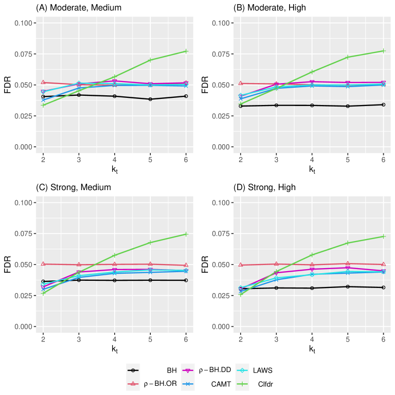
Figure 1: The empirical FDR comparisons for the settings described in the bivariate scenario; $\alpha=0.05$.

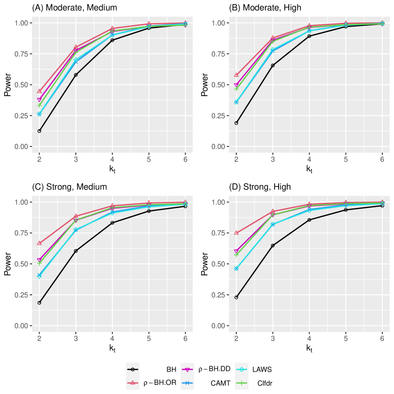
Figure 2: The empirical power comparisons for the settings described in the bivariate scenario; $\alpha=0.05$.

4.2 Univariate side information

Next, we consider the univariate covariate case and generate data according to the following model

$$\begin{split}&\theta_{i}\overset{\text{ind}}{\sim}\text{Bernoulli}\{\pi(i)\},\quad i=1,\ldots,5000,\\ &X_{i}|\theta_{i}\overset{\text{ind}}{\sim}(1-\theta_{i})N(0,1)+\theta_{i}N(\mu,1),\quad i=1,\ldots,5000.\end{split}$$

Two settings are considered. In Setting 1, the signals appear with elevated frequencies in the following blocks:

$$\begin{split}\pi(i)=0.9\ \text{for}\ i\in[1001,1200]\cup[2001,2200];\\ \pi(i)=0.6\ \text{for}\ i\in[3001,3200]\cup[4001,4200].\end{split}$$

For the rest of the locations we set $\pi(i)=0.01$. We vary $\mu$ from 2 to 4 to study the impact of signal strength. In Setting 2, we set $\pi(i)=\pi_{0}$ in the above specified blocks and $\pi(i)=0.01$ elsewhere. We fix $\mu=3$ and vary $\pi_{0}$ from 0.5 to 0.9 to study the influence of sparsity levels. In these two cases, the side information $s_{i}$ can be interpreted as the signal location $i$. When implementing CAMT, we use a spline basis with six equiquantile knots for $\pi(i)$ and $f_{1}(\cdot|i)$ to account for potential complex nonlinear effects as suggested in Zhang and Chen, (2022) and Lei and Fithian, (2018).

Again, we compare the six procedures as in Section 4.1, and the results of Settings 1 and 2 are summarized in the first and second rows of Figure 3, respectively. We can see from the first column of Figure 3 that, in both settings all methods control FDR appropriately at the target level. From the second column, it can be seen that both $\rho$-BH.OR and $\rho$-BH.DD outperform the other four methods. This is due to the fact that, besides the ability in incorporating the sparsity information, the $\rho$-value statistic also adopts other structural knowledge and is henceforth more informative than the p-value based methods. In addition, the nonparametric approach employed by $\rho$-BH.DD is better at capturing non-linear information than the parametric model used in CAMT, and again leads to a more powerful procedure.

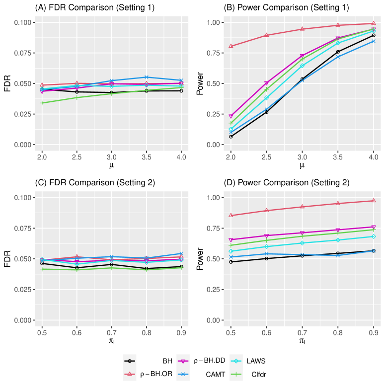
Figure 3: The empirical FDR and Power comparisons for the two settings described in the univariate scenario; $\alpha=0.05$.

5 Data Analysis

In this section, we compare the performance of $\rho$-BH.DD with Clfdr, CAMT, LAWS and BH on two real datasets.

5.1 MWAS data

We first analyze a dataset from a microbiome-wide association study of sex effect (McDonald et al., , 2018), which is available at https://github.com/knightlab-analyses/american-gut-analyses. The aim of the study is to distinguish the abundant bacteria in the gut microbiome between males and females by the sequencing of a fingerprint gene in the bacteria 16S rRNA gene. This dataset is also analyzed in Zhang and Chen, (2022). We follow their preprocessing procedure to obtain 2492 p-values from Wilcoxon rank sum test for different operational taxonomic units (OTUs), and the percentages of zeros across samples for the OTUs are considered as the univariate side information. Because a direct estimation of the non-null distributions of the original Wilcoxon rank sum test statistics is difficult, we construct pseudo z-values by $z_{i}=\Phi^{-1}(p_{i})\times(2B_{i}-1)$, where $B_{i}$’s are independent $\text{Bernoulli}(0.5)$ random variables and $\Phi^{-1}$ is the inverse of standard normal cdf. Then we run $\rho$-BH.DD on those pseudo z-values by employing the same estimation methods of $\pi(\cdot)$ and $f_{1}(\cdot|\cdot)$ as described in Section 4. When implementing CAMT, we use the spline basis with six equiquantile knots as the covariates as recommended in Zhang and Chen, (2022). The results are summarized in Figure 4 (a). We can see that $\rho$-BH.DD rejects significantly more hypotheses than LAWS and BH across all FDR levels. $\rho$-BH.DD also rejects slightly more tests than Clfdr under most FDR levels, and is more stable than CAMT. Because Clfdr may suffer from possible FDR inflation as shown in the simulations, we conclude that $\rho$-BH.DD enjoys the best performance on this dataset.

5.2 ADHD data

We next analyze a preprocessed magnetic resonance imaging (MRI) data for a study of attention deficit hyperactivity disorder (ADHD). The dataset is available at http://neurobureau.projects.nitrc.org/ADHD200/Data.html. We adopt the Gaussian filter-blurred skullstripped gray matter probability images from the Athena Pipline, which are MRI images with a resolution of $197\times 233\times 189$. We pool the 776 training samples and 197 testing samples together, remove 26 samples with no ADHD index, and split the pooled data into one ADHD sample of size 585 and one normal sample of size 362. Then we downsize the resolution of images to $30\times 36\times 30$ by taking the means of pixels within blocks, and then obtain $30\times 36\times 30$ two-sample t-test statistics. Similar data preprocessing strategy is also used in Cai et al., (2022). In such dataset, the 3-dimensional coordinate indices can be employed as the side information. The results of the five methods are summarized in Figure 4 (b). Again, it is obvious to see that $\rho$-BH.DD rejects more hypotheses than CAMT, LAWS, Clfdr and BH across all FDR levels.

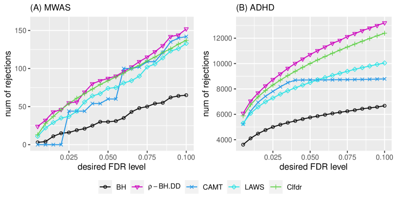
Figure 4: Total numbers of rejections of $\rho$-BH.DD, CAMT, LAWS, Clfdr and BH, respectively for MWAS (Left) and ADHD (Right) datasets.

6 Conclusion and Discussions

This article introduces a novel multiple testing framework based on the newly proposed $\rho$-values. The strength of such framework includes its abilities in unifying the current existing p-values and Lfdr statistics based procedures, as well as in achieving optimal power with much less stringent conditions compared to the Lfdr methods. In the meanwhile it can be extended to incorporate side information through weighting and again the asymptotic optimality can be attained.

As a final message, based on our proposal, we briefly discuss in this section that the frameworks provided by p-values and Lfdr statistics are not as different as claimed in the literature. Note that, a central message of Storey et al., (2007); Sun and Cai, (2007); Leung and Sun, (2021) is that reducing z-values to p-values may lead to substantial information loss. The narrative seems to view Lfdr and p-value as two fundamentally different statistics. However, we have shown in Section 3.1 that $\rho$-value is a special case of p-value but in the meantime $\rho$-value can produce the same ranking as Lfdr. Therefore, a more accurate paraphrasing of the message in Storey et al., (2007); Sun and Cai, (2007) should be that “Statistics that take into account the information from alternative distributions are superior to statistics that do not.”

To be more concrete, we show below that a Lfdr based procedure proposed in Leung and Sun, (2021) is actually a special variation of Algorithm 1 under Model (1). Suppose $f_{1}$ and $f_{0}$ are known but $\pi$ is not. As mentioned in Section 3.3, a natural choice of $\hat{\pi}$ is the Storey estimator. Note that, the Storey estimator requires a predetermined tuning parameter $\tau$. By replacing $\pi$ with $\hat{\pi}$, the threshold in Step 3 of the $\rho$-BH procedure becomes $\rho_{(k)}$ where $k=\max_{j}\left\{(1-\hat{\pi})c(\rho_{(j)})\leq\alpha j/m\right\}.$ In a special case when we allow varying $\tau$ for different $j$ and let $\tau=c(\rho_{(j)})$, then it yields that $k=\max_{j}\left\{\dfrac{\#\{i:c(\rho_{i})\geq 1-c(\rho_{(j)})\}}{j}\leq\alpha\right\}.$ Now if we add $1$ to the numerator and let $k=\max_{j}\left\{\dfrac{1+\#\{i:c(\rho_{i})\geq 1-c(\rho_{(j)})\}}{j}\leq\alpha\right\},$ then the decision rule $\boldsymbol{\delta}=\{\mathbb{I}(\rho_{i}\leq\rho_{(k)})\}_{i=1}^{m}$ is equivalent to the rule given by the ZAP procedure (Leung and Sun, , 2021) that is based on Lfdr. Hence, the ZAP procedure can be viewed as a special case of the $\rho$-BH procedure under Model (1), and can be unified into the proposed $\rho$-BH framework.

Appendix A Data-Driven Weighted $\rho$-BH Procedure

The data-driven version of the weighted $\rho$-BH procedure is described in Algorithm 6.

Algorithm 6 The data-driven weighted $\rho$-BH procedure

Input: $\{X_{i}\}_{i=1}^{m}$; predetermined weights $\{w_{i}\}_{i=1}^{m}$; desired FDR level $\alpha$.

1:Randomly split the data into two disjoint halves $\{X_{i}\}^{m}_{i=1}=\{X_{1,i}\}^{m_{1}}_{i=1}\cup\{X_{2,i}\}^{m_{2}}_{i=1}$, $\{w_{i}\}^{m}_{i=1}=\{w_{1,i}\}^{m_{1}}_{i=1}\cup\{w_{2,i}\}^{m_{2}}_{i=1}$, where $m_{1}=\lfloor m/2\rfloor$.

2:Use $\{X_{1,i}\}^{m_{1}}_{i=1}$ to construct the second half alternative estimate $\hat{f}_{1}^{\scriptscriptstyle(2)}$ and a conservative consistent estimate $\hat{\pi}_{2}$.

3:Run Algorithm 3 with $\{X_{2,i}\}_{i=1}^{m_{2}}$, $\hat{f}_{1}^{\scriptscriptstyle(2)}$, $\hat{\pi}_{2}$, $\{w_{2,i}\}_{i=1}^{m_{2}}$, $\alpha$ as inputs.

4:Switch the roles of $\{X_{1,i}\}^{m_{1}}_{i=1}$, $\{w_{1,i}\}^{m_{1}}_{i=1}$ and $\{X_{2,i}\}^{m_{2}}_{i=1}$, $\{w_{2,i}\}^{m_{2}}_{i=2}$. Repeat Steps 2 to 3 and combine the rejections.

The next theorem provides the theoretical guarantee for the asymptotic mFDR control of Algorithm 6.

Theorem 9.

Assume that $\{X_{i},\theta_{i}\}_{i=1}^{m}$ are independent. Denote by $\{\hat{q}_{d,i}\}_{i=1}^{m_{d}}$, $\hat{q}_{d,(k_{d})}$ and $\hat{\pi}_{d}$ the weighted $\rho$-values, selected thresholds and the estimated alternative proportions obtained from Algorithm 6, for the first and second halves of the data respectively, $d=1,2$. Denote by $\hat{c}_{d}$ the null distribution function for $\hat{\rho}_{d,i}$. Suppose $0\leq\hat{\pi}_{d}\overset{P}{\rightarrow}\tilde{\pi}_{d}\leq\pi$ and let $\tilde{Q}_{d}(t)=\frac{\sum_{i=1}^{m_{d}}(1-\tilde{\pi}_{d})\hat{c}_{d}(w_{d,i}t)}{\mathbb{E}\{\sum_{i=1}^{m_{d}}\mathbb{I}(\hat{q}_{d,i}\leq t)\}}$ and $t_{d,L}=\sup\{t>0:\tilde{Q}_{d}(t)\leq\alpha\}$, $d=1,2$. Based on the notations from Algorithm 6, suppose the following hold

1. $\hat{q}_{d,(k_{d})}\geq\nu$, $\sum_{i=1}^{m_{d}}\mathbb{P}(\hat{q}_{d,i}\leq\nu)\geq cm$, for some constants $\nu,c>0$;

2. $\limsup_{t\rightarrow 0^{+}}\tilde{Q}_{d}(t)<\alpha$, $\liminf_{t\rightarrow\infty}\tilde{Q}_{d}(t)>\alpha$;

3. $\inf_{t\geq t_{d,L}+\epsilon_{t}}\tilde{Q}_{d}(t)\geq\alpha+\epsilon_{\alpha}$, $\tilde{Q}_{d}(t)$ is strictly increasing in $t\in(t_{d,L}-\epsilon_{t},t_{d,L}+\epsilon_{t})$, for some constants $\epsilon_{\alpha},\epsilon_{t}>0$.

Then we have $\lim_{m\rightarrow\infty}\text{mFDR}_{\text{Algorithm }\ref{alg5}}\leq\alpha.$

Appendix B Proofs of Main Theorems and Propositions

Note that Theorems 1 and 4 follow directly from the proof of the original BH procedure as discussed in the main text. Theorem 2 is a special case of Theorem 7. Theorems 3 and 9 are special cases of Theorem 8. Theorem 5 is a special case of Theorem 6. Hence, we focus on the proofs of Proposition 1, Theorem 6, Theorem 7 and Theorem 8 in this section.

To simplify notation, we define a procedure equivalent to Algorithm 4. This equivalence is stated in Lemma 1, whose proof will be given later.

Algorithm 7 A procedure equivalent to Algorithm 4

Input: $\{X_{i}\}_{i=1}^{m}$; $\{s_{i}\}_{i=1}^{m}$; predetermined density functions $\{g(\cdot|s_{i})\}_{i=1}^{m}$; non-null proportions $\{\pi(s_{i})\}_{i=1}^{m}$; predetermined $\{\eta(s_{i})\}_{i=1}^{m}$; desired FDR level $\alpha$.

1:Calculate the $\rho$-values $\rho_{i}=f_{0}(X_{i}|s_{i})/g(X_{i}|s_{i})$; compute the null distribution functions of each $\rho_{i}$, and denote them by $\{c_{i}(\cdot)\}_{i=1}^{m}$.

2:Let $w_{i}=\frac{\eta(s_{i})}{1-\eta(s_{i})}$, and compute the weighted $\rho$-values $q_{i}=\rho_{i}/w_{i}$, $i=1,\ldots,m$.

3:Let $t^{*}=\text{max}_{t\geq 0}\left\{\frac{\sum_{i=1}^{m}\{1-\pi(s_{i})\}c_{i}(w_{i}t)}{\{\sum_{i=1}^{m}\mathbb{I}(q_{i}\leq t)\}\lor 1}\leq\alpha\right\}$. Reject all $H_{0,i}$ with $q_{i}\leq t^{*}$.

Lemma 1.

Algorithm 4 and Algorithm 7 are equivalent in the sense that they reject the same set of hypotheses.

B.1 Proof of Proposition 1

Denote by $\hat{\mathbb{P}}\{c(\rho_{i})>\tau\}:=\dfrac{\sum_{i=1}^{m}\mathbb{I}\{c(\rho_{i})>\tau\}}{m}$. Since $\sum_{i=1}^{m}\mathbb{I}\{c(\rho_{i})>\tau\}$ follows $\text{Binomial}(m,p)$ where $p=\mathbb{P}\{c(\rho_{i})>\tau\}$, we have that

$$\hat{\mathbb{P}}\{c(\rho_{i})>\tau\}\overset{P}{\rightarrow}p.$$

Let $p_{0}=\mathbb{P}\{c(\rho_{i})>\tau|H_{0,i}\}$ and $p_{1}=\mathbb{P}\{c(\rho_{i})>\tau|H_{1,i}\}$, then $p=(1-\pi)p_{0}+\pi p_{1}$. Since $c(\rho_{i})\sim\text{Unif}(0,1)$ under $H_{0,i}$, it follows that $p=(1-\pi)(1-\tau)+\pi p_{1}$. Hence, $1-p/(1-\tau)<\pi$, and the proposition follows. ∎

B.2 Proof of Theorem 6

Proof.

By Lemma 1, we only need to prove the mFDR control for Algorithm 7. Assumption 8 ensures that $Q(t)$ is well defined when $t\geq\nu$. Note that, by Assumption 8 and standard Chernoff bound for independent Bernoulli random variables, we have uniformly for $t\geq\nu$ and any $\epsilon>0$

$$\begin{split}&\mathbb{P}\left(\left|\frac{\sum_{i=1}^{m}\mathbb{I}(q_{i}\leq t)}{\mathbb{E}\{\sum_{i=1}^{m}\mathbb{I}(q_{i}\leq t)\}}-1\right|\geq\epsilon\right)\\ \leq&2e^{-\epsilon^{2}\sum_{i=1}^{m}\mathbb{P}(q_{i}\leq t)/3}\\ \leq&2e^{-\epsilon^{2}\sum_{i=1}^{m}\mathbb{P}(q_{i}\leq\nu)/3}\rightarrow 0,\end{split}$$

which implies

$$\sup_{t\geq\nu}|Q(t)-\widehat{\text{FDP}}(t)|\overset{P}{\rightarrow}0$$ (6)

as $m\rightarrow\infty$, where $\widehat{\text{FDP}}(t)=\frac{\sum_{i=1}^{m}\{1-\pi(s_{i})\}c_{i}(w_{i}t)}{\{\sum_{i=1}^{m}\mathbb{I}(q_{i}\leq t)\}\lor 1}.$

Assumption 9 implies $t_{L}<\infty$. Moreover, combining Equation (6) with Assumption 10, we have $\widehat{\text{FDP}}(t)>\alpha$ for any $t\geq t_{L}+\epsilon_{t}$ with probability going to $1$. Thus, we only have to consider $t<t_{L}+\epsilon_{t}$. Specifically, we consider $t\in(t_{L}-\epsilon_{t},t_{L}+\epsilon_{t})$. As $Q(t)$ is strictly increasing within this range by Assumption 10, we have

$$t^{*}=Q^{-1}\{Q(t^{*})\}\overset{P}{\rightarrow}Q^{-1}\{\widehat{\text{FDP}}(t^{*})\}=Q^{-1}(\alpha)=t_{L}.$$

Therefore, we have

$$\begin{split}\text{mFDR}_{\text{Algorithm }\ref{alg:eqv}}&=\frac{\sum_{i=1}^{m}\mathbb{P}(q_{i}\leq t^{*},\theta_{i}=0)}{\mathbb{E}\{\sum_{i=1}^{m}\mathbb{I}(q_{i}\leq t^{*})\}}\\ &=\frac{\sum_{i=1}^{m}\mathbb{P}(q_{i}\leq t_{L},\theta_{i}=0)}{\mathbb{E}\{\sum_{i=1}^{m}\mathbb{I}(q_{i}\leq t_{L})\}}+o(1)\\ &=Q(t_{L})+o(1)\leq\alpha+o(1).\end{split}$$ (7)

∎

B.3 Proof of Theorem 7

We first state a useful lemma whose proof will be given later.

Lemma 2.

Let $g(\cdot|s_{i})\equiv f_{1}(\cdot|s_{i})$, $i=1,\ldots,m$, $\eta(\cdot)\equiv\pi(\cdot)$. For any $t>0$, let

$$Q(t)=\frac{\sum_{i=1}^{m}\{1-\pi(s_{i})\}c_{i}(w_{i}t)}{\mathbb{E}\{\sum_{i=1}^{m}\mathbb{I}(q_{i}\leq t)\}},\quad t_{L}=\text{sup}\{t\in(0,\infty):Q(t)\leq\alpha\}.$$

Suppose Assumption 11 holds. Then we have

1. $Q(t)<\frac{t}{1+t}$;

2. $Q(t)$ is strictly increasing;

3. $\lim_{m\rightarrow\infty}(\text{ETP}_{\bm{\delta}^{L}}-\text{ETP}_{\bm{\delta}^{\prime}})\geq 0$, for any testing rule $\bm{\delta}^{\prime}$ based on $\{X_{i}\}_{i=1}^{m}$ and $\{s_{i}\}_{i=1}^{m}$ such that $\lim_{m\rightarrow\infty}\text{mFDR}_{\bm{\delta}^{\prime}}\leq\alpha$, where $\bm{\delta}^{L}=\{\mathbb{I}(q_{i}\leq t_{L})\}_{i=1}^{m}$.

Next we prove Theorem 7.

Proof.

By Lemma 1, Algorithm 4 is equivalent to reject all hypotheses that satisfying $q_{i}\leq t^{*}$, where $t^{*}$ is the threshold defined in Algorithm 7. To simplify notations, let $\nu=\frac{\alpha}{1-\alpha}$ and we next show that $t^{*}\geq\nu$ in probability.

By the standard Chernoff bound for independent Bernoulli random variables, we have

$$\begin{split}\mathbb{P}\left(\left|\frac{\sum_{i=1}^{m}\mathbb{I}(q_{i}\leq\nu)}{\sum_{i=1}^{m}\mathbb{P}(q_{i}\leq\nu)}-1\right|\geq\epsilon\right)\leq 2e^{-\epsilon^{2}\sum_{i=1}^{m}\mathbb{P}(q_{i}\leq\nu)/3}\end{split}$$

for all $0<\epsilon<1$. By Assumption 11, the above implies

$$\left|\frac{\sum_{i=1}^{m}\mathbb{I}(q_{i}\leq\nu)}{\sum_{i=1}^{m}\mathbb{P}(q_{i}\leq\nu)}-1\right|=o_{P}(1).$$ (8)

Combining Equation (8) and the first part of Lemma 2, we have

$$\begin{split}\frac{\sum_{i=1}^{m}\{1-\pi(s_{i})\}c_{i}(w_{i}\nu)}{\{\sum_{i=1}^{m}\mathbb{I}(q_{i}\leq\nu)\}\lor 1}=&\frac{\sum_{i=1}^{m}\{1-\pi(s_{i})\}c_{i}(w_{i}\nu)}{\sum_{i=1}^{m}\mathbb{P}(q_{i}\leq\nu)}+o_{P}(1)\\ =&Q(\nu)+o_{P}(1)<\frac{\nu}{1+\nu}+o_{P}(1)\\ =&\alpha+o_{P}(1),\end{split}$$ (9)

which implies $\mathbb{P}(t^{*}\geq\nu)\rightarrow 1$. Therefore, we will only focus the event $\{t^{*}\geq\nu\}$ in the following proof.

For any $t>0$, we let

$$\begin{split}&Q(t)=\frac{\sum_{i=1}^{m}\{1-\pi(s_{i})\}c_{i}(w_{i}t)}{\mathbb{E}\{\sum_{i=1}^{m}\mathbb{I}(q_{i}\leq t)\}},\\ &\widehat{\text{FDP}}(t)=\frac{\sum_{i=1}^{m}\{1-\pi(s_{i})\}c_{i}(w_{i}t)}{\{\sum_{i=1}^{m}\mathbb{I}(q_{i}\leq t)\}\lor 1},\end{split}$$

and

$$\begin{split}&t_{L}=\text{sup}\{t\in(0,\infty):Q(t)\leq\alpha\},\\ &t^{*}=\text{sup}\{t\in(0,\infty):\widehat{\text{FDP}}(t)\leq\alpha\}.\end{split}$$

Following the proof of the third part of Lemma 2, we consider two cases: $\lim\limits_{m\rightarrow\infty}\frac{\pi(s_{i})}{m}\leq 1-\alpha$ and $\lim\limits_{m\rightarrow\infty}\frac{\pi(s_{i})}{m}>1-\alpha$.

The first case is trivial by noting that mFDR can be controlled even if we reject all null hypotheses. For the second case, we need to show that $t^{*}{\overset{P}{\rightarrow}}t_{L}$. Similar to the proof of Equation (8), we have uniformly for $t\geq\nu$ and any $\epsilon>0$,

$$\begin{split}&\mathbb{P}\left(\left|\frac{\sum_{i=1}^{m}\mathbb{I}(q_{i}\leq t)\}}{\mathbb{E}\{\sum_{i=1}^{m}\mathbb{I}(q_{i}\leq t)\}}-1\right|\geq\epsilon\right)\\ \leq&2e^{-\epsilon^{2}\sum_{i=1}^{m}\mathbb{P}(q_{i}\leq t)/3}\\ \leq&2e^{-\epsilon^{2}\sum_{i=1}^{m}\mathbb{P}(q_{i}\leq\nu)/3}\rightarrow 0,\end{split}$$

which implies $|\widehat{\text{FDP}}(t)-Q(t)|\overset{P}{\rightarrow}0$ uniformly in $t\geq\nu$. Thus, $\widehat{\text{FDP}}(t^{*})\overset{P}{\rightarrow}Q(t^{*})$. Moreover, by Lemma 2, we know that $Q(t)$ is continuous and strictly increasing. Therefore, we can define the inverse function $Q^{-1}(\cdot)$ of $Q(\cdot)$. Thus, by the continuous mapping theorem, we have

$$t^{*}=Q^{-1}\{Q(t^{*})\}\overset{P}{\rightarrow}Q^{-1}\{\widehat{\text{FDP}}(t^{*})\}=Q^{-1}(\alpha)=t_{L}.$$

By the third part of Lemma 2, we have $\lim\limits_{m\rightarrow\infty}(\text{ETP}_{\bm{\delta}^{L}}-\text{ETP}_{\bm{\delta}})\geq 0$ and therefore,

$$\begin{split}\lim_{m\rightarrow\infty}\frac{\text{ETP}_{\bm{\delta}_{\rho}}}{\text{ETP}_{\bm{\delta}}}&=\lim_{m\rightarrow\infty}\frac{\text{ETP}_{\bm{\delta}_{\rho}}}{\text{ETP}_{\bm{\delta}_{L}}}\frac{\text{ETP}_{\bm{\delta}_{L}}}{\text{ETP}_{\bm{\delta}}}\geq\lim_{m\rightarrow\infty}\frac{\text{ETP}_{\bm{\delta}_{\rho}}}{\text{ETP}_{\bm{\delta}_{L}}}\\ &=\lim_{m\rightarrow\infty}\frac{\mathbb{E}\{\sum_{i=1}^{m}\theta_{i}\mathbb{I}(\rho_{i}\leq t^{*})\}}{\mathbb{E}\{\sum_{i=1}^{m}\theta_{i}\mathbb{I}(\rho_{i}\leq t_{L})\}}\\ &\geq 1+\lim_{m\rightarrow\infty}\frac{\sum_{i=1}^{m}\{1-\pi(s_{i})\}o(1)}{\sum_{i=1}^{m}\{1-\pi(s_{i})\}c_{i}(w_{i}t_{L})}\geq 1.\\ \end{split}$$

∎

B.4 Proof of Theorem 8

We first introduce Lemma 3, whose proof will be given later.

Lemma 3.

Denote Steps 2 to 3 of Algorithm 5 as ‘Half-procedure’ and we inherit all other notations from Theorem 8. Suppose Assumptions 12-14 hold for $d=2$. Then we have

$$\lim_{m\rightarrow\infty}\text{mFDR}_{\text{Half-procedure}}\leq\alpha.$$

Next we prove Theorem 8.

Proof.

Without loss of generality, we assume $\{X_{1,i}\}^{m_{1}}_{i=1}=\{X_{i}\}^{m_{1}}_{i=1}$ and $\{X_{2,i}\}^{m_{2}}_{i=1}=\{X_{i}\}^{m}_{i=m_{1}+1}$. By Lemma 1 and Lemma 3, we have that

$$\begin{split}&\frac{\mathbb{E}\{\sum_{i=1}^{m_{1}}(1-\theta_{i})\delta_{i}\}}{\mathbb{E}\{\sum_{i=1}^{m_{1}}\delta_{i}\}}\leq\alpha+o(1),\\ &\frac{\mathbb{E}\{\sum_{i=m_{1}+1}^{m}(1-\theta_{i})\delta_{i}\}}{\mathbb{E}\{\sum_{i=m_{1}+1}^{m}\delta_{i}\}}\leq\alpha+o(1).\end{split}$$ (10)

On the other hand, we can decompose $\text{mFDR}_{\bm{\delta}}$ as

$$\begin{split}\text{mFDR}_{\bm{\delta}}=&\frac{\mathbb{E}\{\sum_{i=1}^{m}(1-\theta_{i})\delta_{i}\}}{\mathbb{E}\{\sum_{i=1}^{m}\delta_{i}\}}\\ =&\frac{\mathbb{E}\{\sum_{i=1}^{m_{1}}(1-\theta_{i})\delta_{i}\}}{\mathbb{E}\{\sum_{i=1}^{m}\delta_{i}\}}+\frac{\mathbb{E}\{\sum_{i=m_{1}+1}^{m}(1-\theta_{i})\delta_{i}\}}{\mathbb{E}\{\sum_{i=1}^{m}\delta_{i}\}}\\ =&\frac{\mathbb{E}\{\sum_{i=1}^{m_{1}}(1-\theta_{i})\delta_{i}\}}{\mathbb{E}\{\sum_{i=1}^{m_{1}}\delta_{i}\}}\frac{\mathbb{E}\{\sum_{i=1}^{m_{1}}\delta_{i}\}}{\mathbb{E}\{\sum_{i=1}^{m}\delta_{i}\}}+\\ &\frac{\mathbb{E}\{\sum_{i=m_{1}+1}^{m}(1-\theta_{i})\delta_{i}\}}{\mathbb{E}\{\sum_{i=m_{1}+1}^{m}\delta_{i}\}}\frac{\mathbb{E}\{\sum_{i=m_{1}+1}^{m}\delta_{i}\}}{\mathbb{E}\{\sum_{i=1}^{m}\delta_{i}\}}.\end{split}$$ (11)

Therefore, by Equations (10) and (11), we conclude that

$$\begin{split}\lim_{m\rightarrow\infty}\text{mFDR}_{\bm{\delta}}&\leq\alpha\left\{\frac{\mathbb{E}(\sum_{i=1}^{m_{1}}\delta_{i})}{\mathbb{E}(\sum_{i=1}^{m}\delta_{i})}+\frac{\mathbb{E}(\sum_{i=m_{1}+1}^{m}\delta_{i})}{\mathbb{E}(\sum_{i=1}^{m}\delta_{i})}\right\}=\alpha.\end{split}$$

∎

Appendix C Proofs of Lemmas

C.1 Proof of Lemma 1

Proof.

It is easy to see that $t^{*}\geq q_{(k)}$ as

$$\frac{\sum_{i=1}^{m}\{1-\pi(s_{i})\}c_{i}(w_{i}q_{(k)})}{\sum_{i=1}^{m}\mathbb{I}(q_{i}\leq q_{(k)})}\leq\alpha.$$

Now it suffices to show that, for any $t\geq q_{(k+1)}$, we have

$$\frac{\sum_{i=1}^{m}\{1-\pi(s_{i})\}c_{i}(w_{i}t)}{\sum_{i=1}^{m}\mathbb{I}(q_{i}\leq t)}>\alpha.$$ (12)

By the definition of $k$, for any $l\geq k+1$, we have

$$\frac{\sum_{i=1}^{m}\{1-\pi(s_{i})\}c_{i}(w_{i}q_{(l)})}{\sum_{i=1}^{m}\mathbb{I}(q_{i}\leq q_{(l)})}>\alpha.$$

Then for any $l\geq k+1$, for any $t\in[q_{(l)},q_{(l+1)})$ where $q_{(m+1)}=\infty$, we have

$$\begin{split}\frac{\sum_{i=1}^{m}\{1-\pi(s_{i})\}c_{i}(w_{i}t)}{\sum_{i=1}^{m}\mathbb{I}(q_{i}\leq t)}=&\frac{\sum_{i=1}^{m}\{1-\pi(s_{i})\}c_{i}(w_{i}t)}{l}\\ \geq&\frac{\sum_{i=1}^{m}\{1-\pi(s_{i})\}c_{i}(w_{i}q_{(l)})}{l}\\ =&\frac{\sum_{i=1}^{m}\{1-\pi(s_{i})\}c_{i}(w_{i}q_{(l)})}{\sum_{i=1}^{m}\mathbb{I}(q_{i}\leq q_{(l)})}>\alpha.\end{split}$$

This proves Equation (12) and concludes the proof.

∎

C.2 Proof of Lemma 2

Proof.

First of all, by Assumption 11, we have that $Q(t)$ is well defined for $t\geq\nu$. For any $t$ such that $\mathbb{E}\{\sum_{i=1}^{m}\mathbb{I}(q_{i}\leq t)\}=0$, we set $Q(t)=0$ for simplicity and it will not affect the results. We can rewrite $Q(t)$ as

$$\begin{split}Q(t)&=\frac{\mathbb{E}\{\sum_{i=1}^{m}(1-\theta_{i})\delta_{i}\}}{\mathbb{E}(\sum_{i=1}^{m}\delta_{i})}=\frac{\mathbb{E}[\sum_{i=1}^{m}\mathbb{E}\{(1-\theta_{i})\delta_{i}|X_{i}\}]}{\mathbb{E}(\sum_{i=1}^{m}\delta_{i})}\\ &=\frac{\mathbb{E}[\sum_{i=1}^{m}\delta_{i}\mathbb{E}\{(1-\theta_{i})|X_{i}\}]}{\mathbb{E}(\sum_{i=1}^{m}\delta_{i})}=\frac{\mathbb{E}\left\{\sum_{i=1}^{m}\mathbb{I}(q_{i}\leq t)\frac{q_{i}}{1+q_{i}}\right\}}{\mathbb{E}\{\sum_{i=1}^{m}\mathbb{I}(q_{i}\leq t)\}}.\end{split}$$ (13)

For the first part of this lemma, note that

$$\begin{split}&\mathbb{E}\left\{\sum_{i=1}^{m}\mathbb{I}(q_{i}\leq t)\frac{q_{i}}{1+q_{i}}\right\}-\frac{t}{1+t}\mathbb{E}\left\{\sum_{i=1}^{m}\mathbb{I}(q_{i}\leq t)\right\}\\ &=\mathbb{E}\left\{\sum_{i=1}^{m}\mathbb{I}(q_{i}\leq t)\left(\frac{q_{i}}{1+q_{i}}-\frac{t}{1+t}\right)\right\}\\ &=\mathbb{E}\left\{\sum_{i=1}^{m}\mathbb{I}(q_{i}\leq t)\frac{q_{i}-t}{(1+q_{i})(1+t)}\right\}\leq 0.\end{split}$$

The equality holds if and only if $\mathbb{P}(q_{i}<t|q_{i}\leq t)=0$. Therefore, by Equation (13), we have

$$Q(t)=\frac{\mathbb{E}\left\{\sum_{i=1}^{m}\mathbb{I}(q_{i}\leq t)\frac{q_{i}}{1+q_{i}}\right\}}{\mathbb{E}\{\sum_{i=1}^{m}\mathbb{I}(q_{i}\leq t)\}}<\frac{t}{1+t}.$$ (14)

Denote by $\nu=\frac{\alpha}{1-\alpha}$. By Equation (14), we immediately have $t_{L}\geq\nu$. Therefore, we only consider $t\geq\nu$ in the following proof.

For the second part, let $\nu\leq t_{1}<t_{2}<\infty$, $Q(t_{1})=\alpha_{1}$ and $Q(t_{2})=\alpha_{2}$. From the first part, we learn that $\alpha_{1}<\frac{t_{1}}{1+t_{1}}$. Therefore,

$$\begin{split}Q(t_{2})=&\frac{\mathbb{E}\left\{\sum_{i=1}^{m}\mathbb{I}(q_{i}\leq t_{2})\frac{q_{i}}{1+q_{i}}\right\}}{\mathbb{E}\left\{\sum_{i=1}^{m}\mathbb{I}(q_{i}\leq t_{2})\right\}}\\ =&\frac{\mathbb{E}\left\{\sum_{i=1}^{m}\mathbb{I}(q_{i}\leq t_{1})\frac{q_{i}}{1+q_{i}}\right\}}{\mathbb{E}\{\sum_{i=1}^{m}\mathbb{I}(q_{i}\leq t_{2})\}}+\frac{\mathbb{E}\left\{\sum_{i=1}^{m}\mathbb{I}(t_{1}<q_{i}\leq t_{2})\frac{q_{i}}{1+q_{i}}\right\}}{\mathbb{E}\{\sum_{i=1}^{m}\mathbb{I}(q_{i}\leq t_{2})\}}\\ =&\frac{\mathbb{E}\left\{\sum_{i=1}^{m}\mathbb{I}(q_{i}\leq t_{1})\frac{q_{i}}{1+q_{i}}\right\}}{\mathbb{E}\{\sum_{i=1}^{m}\mathbb{I}(q_{i}\leq t_{1})\}}\frac{\mathbb{E}\{\sum_{i=1}^{m}\mathbb{I}(q_{i}\leq t_{1})\}}{\mathbb{E}\{\sum_{i=1}^{m}\mathbb{I}(q_{i}\leq t_{2})\}}+\\ &\frac{\mathbb{E}\left\{\sum_{i=1}^{m}\mathbb{I}(t_{1}<q_{i}\leq t_{2})\frac{q_{i}}{1+q_{i}}\right\}}{\mathbb{E}\{\sum_{i=1}^{m}\mathbb{I}(q_{i}\leq t_{2})\}}\\ =&\alpha_{1}\frac{\mathbb{E}\{\sum_{i=1}^{m}\mathbb{I}(q_{i}\leq t_{1})\}}{\mathbb{E}\{\sum_{i=1}^{m}\mathbb{I}(q_{i}\leq t_{2})\}}+\frac{\mathbb{E}\left\{\sum_{i=1}^{m}\mathbb{I}(t_{1}<q_{i}\leq t_{2})\frac{q_{i}}{1+q_{i}}\right\}}{\mathbb{E}\{\sum_{i=1}^{m}\mathbb{I}(q_{i}\leq t_{2})\}}\\ \geq&\alpha_{1}\frac{\mathbb{E}\{\sum_{i=1}^{m}\mathbb{I}(q_{i}\leq t_{1})\}}{\mathbb{E}\{\sum_{i=1}^{m}\mathbb{I}(q_{i}\leq t_{2})\}}+\frac{t_{1}}{1+t_{1}}\frac{\mathbb{E}\{\sum_{i=1}^{m}\mathbb{I}(t_{1}<q_{i}\leq t_{2})\}}{\mathbb{E}\{\sum_{i=1}^{m}\mathbb{I}(q_{i}\leq t_{2})\}}\\ >&\alpha_{1}\frac{\mathbb{E}\{\sum_{i=1}^{m}\mathbb{I}(q_{i}\leq t_{1})\}}{\mathbb{E}\{\sum_{i=1}^{m}\mathbb{I}(q_{i}\leq t_{2})\}}+\alpha_{1}\frac{\mathbb{E}\{\sum_{i=1}^{m}\mathbb{I}(t_{1}<q_{i}\leq t_{2})\}}{\mathbb{E}\{\sum_{i=1}^{m}\mathbb{I}(q_{i}\leq t_{2})\}}\\ =&\alpha_{1}=Q(t_{1}).\end{split}$$

For the third part, note that $Q(t)$ here is continuous and increasing when $m\rightarrow\infty$. We consider two cases: $\lim\limits_{m\rightarrow\infty}\frac{\pi(s_{i})}{m}\leq 1-\alpha$ and $\lim\limits_{m\rightarrow\infty}\frac{\pi(s_{i})}{m}>1-\alpha$.

The first case is trivial since it implies $\lim\limits_{t\rightarrow\infty}Q(t)\leq\alpha$ and $t_{L}=\infty$. The procedure rejects all hypotheses and is obviously most powerful. For the second case, we have $\lim_{t\rightarrow\infty}Q(t)=\frac{\sum_{i=1}^{m}\{1-\pi(s_{i})\}}{m}>\alpha$. Combining this with the fact that $Q(\nu)<\alpha$, we can always find a unique $t_{L}$ such that $Q(t_{L})=\alpha$. Note that, by

$$\begin{split}&\lim_{m\rightarrow\infty}\text{mFDR}_{\bm{\delta}^{L}}=\lim_{m\rightarrow\infty}\frac{\mathbb{E}\left\{\sum_{i=1}^{m}\mathbb{I}(q_{i}\leq t_{L})\frac{q_{i}}{1+q_{i}}\right\}}{\mathbb{E}\{\sum_{i=1}^{m}\mathbb{I}(q_{i}\leq t_{L})\}}=\alpha,\\ \text{and}\ &\lim_{m\rightarrow\infty}\text{mFDR}_{\bm{\delta}^{\prime}}=\lim_{m\rightarrow\infty}\frac{\mathbb{E}\left\{\sum_{i=1}^{m}\delta_{i}^{\prime}\frac{q_{i}}{1+q_{i}}\right\}}{\{\mathbb{E}\sum_{i=1}^{m}\delta_{i}^{\prime}\}}\leq\alpha,\end{split}$$

we have

$$\begin{split}&\lim_{m\rightarrow\infty}\mathbb{E}\left\{\sum_{i=1}^{m}\delta_{i}^{L}\left(\frac{q_{i}}{1+q_{i}}-\alpha\right)\right\}=0\\ \text{and}\ &\lim_{m\rightarrow\infty}\mathbb{E}\left\{\sum_{i=1}^{m}\delta_{i}^{\prime}\left(\frac{q_{i}}{1+q_{i}}-\alpha\right)\right\}\leq 0,\end{split}$$

which implies

$$\lim_{m\rightarrow\infty}\mathbb{E}\left\{\sum_{i=1}^{m}(\delta_{i}^{L}-\delta_{i}^{\prime})\left(\frac{q_{i}}{1+q_{i}}-\alpha\right)\right\}\geq 0.$$ (15)

Note that, by the law of total expectation as in Equation (13), we have

$$\begin{split}&\lim_{m\rightarrow\infty}\{\mathbb{E}(\sum_{i=1}^{m}\delta_{i}^{L}\theta_{i})-\mathbb{E}(\sum_{i=1}^{m}\delta_{i}^{\prime}\theta_{i})\}\geq 0\\ \Leftrightarrow\ &\lim_{m\rightarrow\infty}\mathbb{E}\left\{\sum_{i=1}^{m}(\delta_{i}^{L}-\delta_{i}^{\prime})\frac{1}{1+q_{i}}\right\}\geq 0.\end{split}$$ (16)

Hence, it suffices to show $\lim_{m\rightarrow\infty}\mathbb{E}\left\{\sum_{i=1}^{m}(\delta_{i}^{L}-\delta_{i}^{\prime})\frac{1}{1+q_{i}}\right\}\geq 0.$ By Equation (15), it suffices to show that there exists some $\lambda\geq 0$ such that $(\delta_{i}^{L}-\delta_{i}^{\prime})\frac{1}{1+q_{i}}\geq\lambda(\delta_{i}^{L}-\delta_{i}^{\prime})\left(\frac{q_{i}}{1+q_{i}}-\alpha\right)$ for every $i$, i.e.,

$$(\delta_{i}^{L}-\delta_{i}^{\prime})\left\{\frac{1}{1+q_{i}}-\lambda\left(\frac{q_{i}}{1+q_{i}}-\alpha\right)\right\}\geq 0.$$ (17)

By the first part of this lemma, we have $\alpha=Q(t_{L})<\frac{t_{L}}{1+t_{L}}$ and thus $\frac{1}{t_{L}-\alpha(1+t_{L})}>0$. Let $\lambda=\frac{1}{t_{L}-\alpha(1+t_{L})}$, then for each $i$:

1. If $\delta_{i}^{L}=0$, we have $\delta_{i}^{L}-\delta_{i}^{\prime}\leq 0$ and $q_{i}>t_{L}$. Therefore, $\left\{\frac{1}{1+q_{i}}-\lambda\left(\frac{q_{i}}{1+q_{i}}-\alpha\right)\right\}<\left\{\frac{1}{1+t_{L}}-\lambda\left(\frac{t_{L}}{1+t_{L}}-\alpha\right)\right\}=0$.

2. If $\delta_{i}^{L}=1$, we have $\delta_{i}^{L}-\delta_{i}^{\prime}\geq 0$ and $q_{i}\leq t_{L}$. Therefore, $\left\{\frac{1}{1+q_{i}}-\lambda\left(\frac{q_{i}}{1+q_{i}}-\alpha\right)\right\}\geq\left\{\frac{1}{1+t_{L}}-\lambda\left(\frac{t_{L}}{1+t_{L}}-\alpha\right)\right\}=0$.

This proves Equation (17) and concludes the proof. ∎

C.3 Proof of Lemma 3

Proof.

For $t\geq 0$, we let

$$Q_{2}(t)=\frac{\sum_{i=1}^{m_{2}}\{1-\pi(s_{2,i})\}\hat{c}_{2,i}(w_{2,i}t)}{\mathbb{E}\{\sum_{i=1}^{m_{2}}\mathbb{I}(\hat{q}_{2,i}\leq t)\}},$$

$$\hat{Q}_{2}(t)=\frac{\sum_{i=1}^{m_{2}}\{1-\hat{\pi}_{2}(s_{2,i})\}\hat{c}_{2,i}(w_{2,i}t)}{\mathbb{E}\{\sum_{i=1}^{m_{2}}\mathbb{I}(\hat{q}_{2,i}\leq t)\}},$$

$$\widehat{\text{FDP}}_{2}(t)=\frac{\sum_{i=1}^{m_{2}}\{1-\hat{\pi}_{2}(s_{2,i})\}\hat{c}_{2,i}(w_{2,i}t)}{\{\sum_{i=1}^{m_{2}}\mathbb{I}(\hat{q}_{2,i}\leq t)\}\lor 1},$$

$$t^{*}_{2}=\text{sup}\{t\in[0,\infty):\widehat{\text{FDP}}(t)\leq\alpha\}.$$

As $t^{*}_{2}\geq\hat{q}_{2,(k)}\geq\nu$ by the first part of Assumption 12 and Lemma 1, we only consider $t\geq\nu$ in the following proof. The second part of Assumptiont 12 implies $\mathbb{E}\{\sum_{i=1}^{m_{2}}\mathbb{I}(\hat{q}_{2,i}\leq t)\}\rightarrow\infty$ when $m\rightarrow\infty$ for $t\geq\nu$, which makes $Q_{2}(t)$, $\hat{Q}_{2}(t)$, $\tilde{Q}_{2}(t)$ well defined when $t\geq\nu$.

Note that, by Assumption 12 and the standard Chernoff bound for independent Bernoulli random variables, we have uniformly for $t\geq\nu$ and any $\epsilon>0$

$$\begin{split}&\mathbb{P}\left(\left|\frac{\sum_{i=1}^{m_{2}}\mathbb{I}(\hat{q}_{2,i}\leq t)}{\mathbb{E}\{\sum_{i=1}^{m_{2}}\mathbb{I}(\hat{q}_{2,i}\leq t)\}}-1\right|\geq\epsilon\right)\\ \leq&2e^{-\epsilon^{2}\sum_{i=1}^{m}\mathbb{P}(\hat{q}_{2,i}\leq t)/3}\\ \leq&2e^{-\epsilon^{2}\sum_{i=1}^{m}\mathbb{P}(\hat{q}_{2,i}\leq\nu)/3}\rightarrow 0,\end{split}$$

which implies

$$\sup_{t\geq\nu}|\hat{Q}_{2}(t)-\widehat{\text{FDP}}_{2}(t)|\overset{P}{\rightarrow}0$$ (18)

as $m_{2}\rightarrow\infty$. On the other hand, we have uniformly for $t\geq\nu$,

$$\begin{split}|\hat{Q}_{2}(t)-\tilde{Q}_{2}(t)|=&\left|\frac{\sum_{i=1}^{m_{2}}\{\tilde{\pi}_{2}(s_{2,i})-\hat{\pi}_{2}(s_{2,i})\}\hat{c}_{2,i}(w_{2,i}t)}{\mathbb{E}\{\sum_{i=1}^{m_{2}}\mathbb{I}(\hat{q}_{2,i}\leq t)\}}\right|\\ \leq&\frac{|\sum_{i=1}^{m_{2}}\{\tilde{\pi}_{2}(s_{2,i})-\hat{\pi}_{2}(s_{2,i})\}|}{\mathbb{E}\{\sum_{i=1}^{m_{2}}\mathbb{I}(\hat{q}_{2,i}\leq\nu)\}}\\ =&\frac{m_{2}\times o_{P}(1)}{m_{2}}=o_{P}(1),\end{split}$$

where the first $o_{P}(1)$ is with regard to $m_{1}\rightarrow\infty$ by the uniformly conservative consistency of $\hat{\pi}_{2}(\cdot)$, and the term $m_{2}$ in the denominator comes from the first part of Assumption 12. As the data splitting strategy ensures $m_{1}\approx m_{2}$, we obtain the second $o_{P}(1)$ with regard to $m\rightarrow\infty$. Thus, we have

$$\sup_{t\geq\nu}|\hat{Q}_{2}(t)-\tilde{Q}_{2}(t)|\rightarrow 0$$ (19)

in probability as $m\rightarrow\infty$.

Combining Equations (18) and (19), we have

$$\sup_{t\geq\nu}|\widehat{\text{FDP}}_{2}(t)-\tilde{Q}_{2}(t)|\rightarrow 0$$

in probability as $m\rightarrow\infty$. Then, following the proof of Theorem 6, we can similarly obtain $t^{*}_{2}\rightarrow t_{2,L}$ in probability by Assumptions 13 and 14. Finally, we have

$$\begin{split}\text{mFDR}_{\text{Half-procedure}}&=\frac{\sum_{i=1}^{m_{2}}\mathbb{P}(\hat{q}_{2,i}\leq t^{*}_{2},\theta_{i}=0)}{\mathbb{E}\{\sum_{i=1}^{m_{2}}\mathbb{I}(\hat{q}_{2,i}\leq t^{*}_{2})\}}\\ &=\frac{\sum_{i=1}^{m_{2}}\mathbb{P}(\hat{q}_{2,i}\leq t_{2,L},\theta_{i}=0)}{\mathbb{E}\{\sum_{i=1}^{m_{2}}\mathbb{I}(\hat{q}_{2,i}\leq t_{2,L})\}}+o(1)\\ &=Q_{2}(t_{2,L})+o(1)\leq\tilde{Q}_{2}(t_{2,L})+o(1)\\ &\leq\alpha+o(1).\end{split}$$

∎

References

• Aubert etย al., (2004) Aubert, J., Bar-Hen, A., Daudin, J.-J., and Robin, S. (2004). Determination of the differentially expressed genes in microarray experiments using local fdr. BMC bioinformatics, 5(1):1โ€“9.
• Basu etย al., (2018) Basu, P., Cai, T.ย T., Das, K., and Sun, W. (2018). Weighted false discovery rate control in large-scale multiple testing. Journal of the American Statistical Association, 113(523):1172โ€“1183.
• Benjamini and Hochberg, (1995) Benjamini, Y. and Hochberg, Y. (1995). Controlling the false discovery rate: a practical and powerful approach to multiple testing. Journal of the Royal Statistical Society: Series B (Methodological), 57(1):289โ€“300.
• Benjamini and Hochberg, (1997) Benjamini, Y. and Hochberg, Y. (1997). Multiple hypotheses testing with weights. Scandinavian Journal of Statistics, 24(3):407โ€“418.
• Benjamini and Yekutieli, (2001) Benjamini, Y. and Yekutieli, D. (2001). The control of the false discovery rate in multiple testing under dependency. Annals of Statistics, 29(4):1165โ€“1188.
• Cai etย al., (2019) Cai, T.ย T., Sun, W., and Wang, W. (2019). Covariate-assisted ranking and screening for large-scale two-sample inference. Journal of the Royal Statistical Society Series B: Statistical Methodology, 81(2):187โ€“234.
• Cai etย al., (2022) Cai, T.ย T., Sun, W., and Xia, Y. (2022). Laws: A locally adaptive weighting and screening approach to spatial multiple testing. Journal of the American Statistical Association, 117(539):1370โ€“1383.
• Cao etย al., (2022) Cao, H., Chen, J., and Zhang, X. (2022). Optimal false discovery rate control for large scale multiple testing with auxiliary information. The Annals of Statistics, 50(2):807โ€“857.
• Chen, (2019) Chen, X. (2019). Uniformly consistently estimating the proportion of false null hypotheses via lebesgueโ€“stieltjes integral equations. Journal of Multivariate Analysis, 173:724โ€“744.
• Dobriban etย al., (2015) Dobriban, E., Fortney, K., Kim, S.ย K., and Owen, A.ย B. (2015). Optimal multiple testing under a gaussian prior on the effect sizes. Biometrika, 102(4):753โ€“766.
• Efron, (2003) Efron, B. (2003). Robbins, empirical bayes and microarrays. The Annals of Statistics, 31(2):366โ€“378.
• Efron, (2004) Efron, B. (2004). Large-scale simultaneous hypothesis testing: the choice of a null hypothesis. Journal of the American Statistical Association, 99(465):96โ€“104.
• Efron and Tibshirani, (2007) Efron, B. and Tibshirani, R. (2007). On testing the significance of sets of genes. The Annals of Applied Statistics, 1(1):107โ€“129.
• Efron etย al., (2001) Efron, B., Tibshirani, R., Storey, J.ย D., and Tusher, V. (2001). Empirical bayes analysis of a microarray experiment. Journal of the American Statistical Association, 96(456):1151โ€“1160.
• Fu etย al., (2022) Fu, L., Gang, B., James, G.ย M., and Sun, W. (2022). Heteroscedasticity-adjusted ranking and thresholding for large-scale multiple testing. Journal of the American Statistical Association, 117(538):1028โ€“1040.
• Gang etย al., (2023) Gang, B., Sun, W., and Wang, W. (2023). Structureโ€“adaptive sequential testing for online false discovery rate control. Journal of the American Statistical Association, 118(541):732โ€“745.
• Genovese and Wasserman, (2002) Genovese, C. and Wasserman, L. (2002). Operating characteristics and extensions of the false discovery rate procedure. Journal of the Royal Statistical Society: Series B (Statistical Methodology), 64(3):499โ€“517.
• Genovese etย al., (2006) Genovese, C.ย R., Roeder, K., and Wasserman, L. (2006). False discovery control with p-value weighting. Biometrika, 93(3):509โ€“524.
• Ignatiadis and Huber, (2021) Ignatiadis, N. and Huber, W. (2021). Covariate powered cross-weighted multiple testing. Journal of the Royal Statistical Society Series B: Statistical Methodology, 83(4):720โ€“751.
• Jin and Cai, (2007) Jin, J. and Cai, T.ย T. (2007). Estimating the null and the proportion of nonnull effects in large-scale multiple comparisons. Journal of the American Statistical Association, 102(478):495โ€“506.
• Lei and Fithian, (2018) Lei, L. and Fithian, W. (2018). Adapt: an interactive procedure for multiple testing with side information. Journal of the Royal Statistical Society: Series B (Statistical Methodology), 80(4):649โ€“679.
• Leung and Sun, (2021) Leung, D. and Sun, W. (2021). Zap: $z$-value adaptive procedures for false discovery rate control with side information. arXiv preprint arXiv:2108.12623.
• Li and Barber, (2019) Li, A. and Barber, R.ย F. (2019). Multiple testing with the structure-adaptive benjaminiโ€“hochberg algorithm. Journal of the Royal Statistical Society Series B: Statistical Methodology, 81(1):45โ€“74.
• Liang etย al., (2023) Liang, Z., Cai, T.ย T., Sun, W., and Xia, Y. (2023). Locally adaptive algorithms for multiple testing with network structure, with application to genome-wide association studies. arXiv preprint arXiv:2203.11461.
• Ma etย al., (2022) Ma, L., Xia, Y., and Li, L. (2022). Napa: Neighborhood-assisted and posterior-adjusted two-sample inference. arXiv preprint arXiv:2201.10043.
• McDonald etย al., (2018) McDonald, D., Hyde, E., Debelius, J.ย W., Morton, J.ย T., Gonzalez, A., Ackermann, G., Aksenov, A.ย A., Behsaz, B., Brennan, C., Chen, Y., etย al. (2018). American gut: an open platform for citizen science microbiome research. Msystems, 3(3):10โ€“1128.
• Meinshausen and Rice, (2006) Meinshausen, N. and Rice, J. (2006). Estimating the proportion of false null hypotheses among a large number of independently tested hypotheses. The Annals of Statistics, 34(1):373โ€“393.
• Roquain and Van Deย Wiel, (2009) Roquain, E. and Van Deย Wiel, M.ย A. (2009). Optimal weighting for false discovery rate control. Electronic Journal of Statistics, 3:678โ€“711.
• Storey, (2002) Storey, J.ย D. (2002). A direct approach to false discovery rates. Journal of the Royal Statistical Society: Series B (Statistical Methodology), 64(3):479โ€“498.
• Storey etย al., (2007) Storey, J.ย D., Dai, J.ย Y., and Leek, J.ย T. (2007). The optimal discovery procedure for large-scale significance testing, with applications to comparative microarray experiments. Biostatistics, 8(2):414โ€“432.
• Sun and Cai, (2007) Sun, W. and Cai, T.ย T. (2007). Oracle and adaptive compound decision rules for false discovery rate control. Journal of the American Statistical Association, 102(479):901โ€“912.
• Vovk and Wang, (2021) Vovk, V. and Wang, R. (2021). E-values: Calibration, combination and applications. The Annals of Statistics, 49(3):1736โ€“1754.
• Wang and Ramdas, (2022) Wang, R. and Ramdas, A. (2022). False discovery rate control with e-values. Journal of the Royal Statistical Society Series B: Statistical Methodology, 84(3):822โ€“852.
• Xie etย al., (2011) Xie, J., Cai, T.ย T., Maris, J., and Li, H. (2011). Optimal false discovery rate control for dependent data. Statistics and Its Interface, 4(4):417.
• Zhang and Chen, (2022) Zhang, X. and Chen, J. (2022). Covariate adaptive false discovery rate control with applications to omics-wide multiple testing. Journal of the American Statistical Association, 117(537):411โ€“427.