Scalable Causal Structure Learning via Amortized Conditional Independence Testing

Abstract

Controlling false positives (Type I errors) through statistical hypothesis testing is a foundation of modern scientific data analysis. Existing causal structure discovery algorithms either do not provide Type I error control or cannot scale to the size of modern scientific datasets. We consider a variant of the causal discovery problem with two sets of nodes, where the only edges of interest form a bipartite causal subgraph between the sets. We develop Scalable Causal Structure Learning (SCSL), a method for causal structure discovery on bipartite subgraphs that provides Type I error control. SCSL recasts the discovery problem as a simultaneous hypothesis testing problem and uses discrete optimization over the set of possible confounders to obtain an upper bound on the test statistic for each edge. Semi-synthetic simulations demonstrate that SCSL scales to handle graphs with hundreds of nodes while maintaining error control and good power. We demonstrate the practical applicability of the method by applying it to a cancer dataset to reveal connections between somatic gene mutations and metastases to different tissues.

1Department of Statistics and Data Science, Carnegie Mellon University

2Department of Statistics, University of Michigan

3Computational Oncology, Memorial Sloan Kettering Cancer Center

February 27, 2024

Many scientific applications can be posed as a causal discovery problem where a directed acylic graph (DAG) is learned that models the causal dependencies within an observational dataset (e.g. Tennant et al. [2020], Ogburn et al. [2022]). In order to ensure the reliability of these findings, controlling the error rate on the set of causal discoveries is critical. Given finite data and noisy observations, exact determination of causal arrows in a DAG is impossible. As such, the causal discovery task is typically cast through the lens of statistical hypothesis testing for conditional independencies [Spirtes et al., 2000].

Although the problem of large-scale multiple hypothesis testing and uncertainty quantification is well studied in settings where purely associative relationships are the target discoveries [Benjamini and Hochberg, 1995, Goeman and Solari, 2014], large-scale causal learning produces a unique set of challenges. The number of possible DAGs scales superexponentially with the number of nodes in a graph, making causal learning an especially difficult problem when the number of variables in a dataset is large. Moreover, existing causal structure learning algorithms learn a graph with either no attempt to provide frequentist error guarantees [Chickering, 2003, Ramsey et al., 2017a, Zheng et al., 2018, Cundy et al., 2021b, Annadani et al., 2021, Cundy et al., 2021a] or require parametric assumptions on the data generating distribution which are often unknown in practice [Strobl et al., 2019].

A feature of many scientific datasets that can be exploited to decrease the computational burden of this task is temporal separation of variables. If a dataset has a sequence of variables that measure quantities that came into existence at different times, this corresponds to a priori knowledge that some edges can only be oriented in a particular direction. This allows us to reduce the number of conditional independence tests required to draw an edge on a causal graph.

In this paper, we introduce Scalable Causal Structure Learning (SCSL), a method for large-scale causal hypothesis testing that can scale to problems with hundreds of variables and thousands of potential edges for causal graphs with temporally separated sets of nodes. SCSL enables the use of black box machine learning models for hypothesis testing, requires no parametric assumptions, and returns a $p$-value for each edge under consideration. To scale to large graphs, SCSL recasts the causal search process as a discrete optimization problem. It then amortizes the dominant cost in causal structure identification: conditional independence testing over the combinatorial set of possible parent nodes in the causal graph. This avoids the combinatorial explosion in the candidate conditioning sets and reduces the search to a series of parallelizable optimization problems for each edge. We validate SCSL through semi-synthetic experiments using a cancer dataset that pairs genomic mutations at the primary tumor location of a cancer patient with information about metastases that have developed elsewhere in a patient’s body [Nguyen et al., 2022]. These simulation studies indicate that the method has high power, controls Type I error rate at the target level, and scales to larger graphs than existing methods.

Background and related work

Classical algorithms for causal discovery like the SGS and PC algorithms (Spirtes et al. [2000]) convert causal structure learning into queries of conditional independence between nodes. The SGS algorithm draws an edge between two nodes if they are conditionally dependent given any possible subset of the remaining nodes. The PC algorithm simplifies this process by first deleting edges in the causal graph based on marginal independence testing. The size of the conditioning subsets is then allowed to increase by one for each subsequent round of CI testing, but fewer CI tests are required in each round as the algorithm only considers conditioning subsets of nodes that have remained adjacent to each other. The computational complexity of SGS matches the complexity of the PC in the worst case, but in most settings where the causal graph is reasonably sparse, the PC algorithm significantly reduces the number of independence tests needed to learn a causal graph. Nevertheless, both methods rely on perfect knowledge of the CI structure and are computationally intractable beyond a few dozen nodes. The work of Strobl et al. [2019] extends the PC algorithm to generate edge-specific $p$-values, but only with provable Type I error control under the assumption of zero Type II error during the edge deletion stage of skeleton discovery. Other works take the PC algorithm as a starting point and then relaxes assumptions around faithfulness (e.g. Ramsey et al. [2006]) or causal sufficiency (e.g. Spirtes [2001]), but these methods also rely on having perfect knowledge of the graph’s CI structure.

Other approaches to causal network learning are score-based methods which seek to maximize a score function such as BIC [D and Heckerman, 1997] or BDeau [Heckerman et al., 1995] by searching over the space of DAGs. Since the number of DAGs increases superexponentially with the number of nodes, approximate algorithms based on greedy search [Chickering, 2003, Ramsey et al., 2017a], coordinate descent [Aragam and Zhou, 2015, Fu and Zhou, 2013] or other methods are required. Alternatively, parametric approaches using structural equation modelling (e.g. Shimizu et al. [2011]) can be employed to simplify the task. However, these methods require strict modelling assumptions about the relationship between variables and distribution of errors that are unlikely to hold in practice.

More recently, differentiable approaches to causal discovery have been proposed [Zheng et al., 2018], many of which enable Bayesian inference of the posterior distribution over DAGs [Cundy et al., 2021b, Annadani et al., 2021, Cundy et al., 2021a]. Unfortunately, these methods focus primarily on continuous rather than discrete data, limiting the application to datasets like the cancer dataset we consider in our simulations. Further, Bayesian uncertainty requires accurate model specification for valid posterior coverage. When the model is misspecified, Bayesian credible intervals can massively inflate Type I error. Similarly, Peters et al. [2016] weaken the faithfulness assumptions, but require repeated observations of variables across different intervention settings instead of relying on purely observational data. Overall, no method exists that is capable of providing Type I error control on individual edges across a large graph without making stringent parametric assumptions.

1 Methodology

Consider a directed acyclic graph (DAG) $\mathcal{G}$ with two sets of nodes, $\mathcal{X}$ and $\mathcal{Y}$, where we want to learn the directed edges between $\mathcal{X}$ and $\mathcal{Y}$ from observational data. We assume that we have prior knowledge that no edge is directed from $\mathcal{Y}$ to $\mathcal{X}$ such as temporal separation between the sets of nodes. For instance, in the cancer dataset, $\mathcal{Y}$ would represent metastasis events that occur after the tumors represented by $\mathcal{X}$ were sequenced.

The problem reduces to learning which $X_{j}\in\mathcal{X}$ are connected to which $Y_{k}\in\mathcal{Y}$. A naive approach might be to infer an edge based on a conditional independence test of $X_{j}\perp\!\!\!\perp Y_{k}|\{X_{-j},Y_{-k}\}$ where $X_{-j}:=\mathcal{X}\setminus X_{j}$ and $Y_{-k}:=\mathcal{Y}\setminus Y_{k}$. However, a collider being present in $\mathcal{Y}$ could introduce dependence even when there is no edge present as Figure 1 demonstrates.

Figure 1: $\mathcal{X}=\{X_{1},X_{2}\}$ and $\mathcal{Y}=\{Y_{1},Y_{2}\}$. $Y_{1}$ is a collider, so a conditional independence test would indicate $X_{1}$ and $Y_{2}$ are conditionally dependent given $\{X_{1},Y_{1}\}$. Testing the marginal association in addition would show that $X_{1}\perp\!\!\!\perp Y_{2}$, preventing an edge from being drawn.

We make the following assumptions about the graph and distribution of the data which are common in the literature [Spirtes et al., 2000].

Assumption 1.1 (Global directed Markov property).

For a graph $\mathcal{G}$, if two nodes $U$ and $V$ are d-separated given a disjoint set nodes $W$, then $U$ and $V$ are conditionally independent given $W$.

Assumption 1.2 (d-separation Faithfulness).

For a graph $\mathcal{G}$, if two nodes $U$ and $V$ are conditionally independent given a disjoint set of nodes $W$, then $U$ and $V$ are d-separated given $W$.

Assumption 1.3 (Causal sufficiency).

The graph $\mathcal{G}$ includes all common causes for any pair of nodes contained in $\mathcal{G}$.

These assumptions lead to Proposition 1.4 which is a direct consequence of Proposition 1 in Strobl et al. [2019] combined with the assumption that no edges can be oriented from $\mathcal{Y}$ to $\mathcal{X}$ due to their separation in time.

Proposition 1.4.

Assume $\mathcal{G}$ satisfies the global directed Markov property and the probability distribution is d-separation faithful. Furthermore, assume that edges may not be directed from any element in $\mathcal{Y}$ to any element in $\mathcal{X}$. Then there is an edge between two vertices $X_{j}\in\mathcal{X}$ and $Y_{k}\in\mathcal{Y}$ if and only if $X_{j}$ and $Y_{k}$ are conditionally dependent given $S\cup X_{-j}$ for all $S\subseteq Y_{-k}$.

In order to construct a p-value, we consider a hypothesis test for each pair $(X_{j},Y_{k})$ as follows:

$$\begin{split}&H_{0}:X_{j}\rightarrow Y_{k}\text{ is absent,}\\ &H_{1}:X_{j}\rightarrow Y_{k}\text{ is present.}\end{split}$$ (1)

Proposition 1.4 lets us restate the null and alternative as

$$\begin{split}&H_{0}:\exists S\subseteq\mathcal{Y}\setminus Y_{k}\text{ such that }X_{j}\perp\!\!\!\perp Y_{k}|S,X_{-j},\\ &H_{1}:X_{j}\not\perp\!\!\!\perp Y_{k}|S,X_{-j}\text{ for all }S\subseteq Y_{-k}.\\ \end{split}$$ (2)

Let $p_{X_{j}\perp\!\!\!\perp Y_{k}|S}$ denote the p-value corresponding to a test for conditional independence between $X_{j}$ and $Y_{k}$ given a set of nodes $S$. Equation 2 implies that the p-value $p_{X_{j}\rightarrow Y_{k}}$ can be bounded by

$$p_{X_{j}\rightarrow Y_{k}}\leq\max_{S\subseteq Y_{-k}}p_{X_{j}\perp\!\!\!\perp Y_{k}|S,X_{-j}}.$$ (3)

Constructing a $p$-value to test $H_{0}$ thus reduces to computing $p$-values for a series of conditional independence tests.

1.1 Conditional Independence Testing

To test the null hypothesis that $X_{j}\perp\!\!\!\perp Y_{k}|S,X_{-j}$, we employ the generalized covariance measure (GCM) of Shah and Peters [2020]. The GCM recasts the problem of conditional independence into one about functional estimation of the expected conditional covariance

$$\begin{split}\mathbb{E}\left[\text{Cov}\left(X_{j},Y_{k}|S,X_{-j}\right)\right]:=&\mathbb{E}[\mathbb{E}[X_{j}Y_{k}|S,X_{-j}]\\ -&\mathbb{E}[X_{j}|S,X_{-j}]\mathbb{E}[Y_{k}|S,X_{-j}]],\end{split}$$ (4)

and then tests whether this quantity is equal to $0$. Any set of joint densities for $(\mathcal{X},\mathcal{Y})$ that are null will have this property, although it is possible for $X_{j}$ and $Y_{k}$ to be conditionally dependent but with $0$ covariance. Therefore, this measure will only have power against the set of alternatives which have non-zero conditional covariance, which is likely to be the case in most practical settings.

The procedure constructs a test for the null hypothesis of $0$ conditional covariance by first finding estimates $\hat{X}_{j}$ for the conditional expectation $\mathbb{E}[X_{j}|Y_{S},X_{-j}]$ and $\hat{Y}_{k}$ for the conditional expectation $\mathbb{E}[Y_{k}|Y_{S},X_{-j}]$. Any type of predictive modeling to construct this estimate is valid, for example construction of a neural net, so long as the product of the mean square errors of the two quantities is $o(n^{-1})$. Given $n$ samples $\{X_{j}^{i},Y_{k}^{i},S^{i},X_{-j}^{i}\}_{i=1}^{n}$, we denote $R_{i}=\left(X_{j}^{i}-\widehat{X}_{j}^{i}\right)\left(Y_{k}^{i}-\widehat{Y}_{k}^{i}\right)$, and the test statistic

$$T^{(n)}=\frac{\sqrt{n}\cdot\frac{1}{n}\sum_{i=1}^{n}R_{i}}{\left(\frac{1}{n}\sum_{i=1}^{n}R_{i}^{2}-\left(\frac{1}{n}\sum_{r=1}^{n}R_{r}\right)^{2}\right)^{1/2}},$$ (5)

which will be distributed asymptotically as $\mathcal{N}(0,1)$ under the null, allowing us to construct a valid $p$-value. For a precise account of the technical conditions for the theorem, see Theorem 6 of Shah and Peters [2020] which we recall in the Appendix for completeness.

We note that our method is adaptable to other CI testing procedures such as conditional randomization tests (e.g. Candes et al. [2016], Tansey et al. [2022], Liu et al. [2021]). We focus on the GCM in this work because it requires less stringent modeling assumptions on the conditional distribution $X|Z$ and is less computationally burdensome.

1.2 Amortized Predictive Modeling

The GCM only requires the computation of a single test statistic per conditional independence query. While the computation of the individual test statistics is straightforward, this approach may still become computationally onerous when testing for the presence of an edge using Equation 3 due to the fact that two separate predictive models need to be created for each of the $2^{|\mathcal{Y}|-1}$ CI tests corresponding to $H_{0}$ which will cause this methodology to scale poorly as $|\mathcal{Y}|$ increases.

To make this process more computationally tractable, we will create a single predictive model for each element $Y_{k}\in\mathcal{Y}$ that has the flexibility to take in a choice of conditioning set $S\subseteq Y_{-k}$ as well as a choice of element $X_{j}\in\mathcal{X}$ and outputs an estimate of $\mathbb{E}[Y_{k}|X_{-j},S]$. We call this amortized predictive modeling because instead of creating bespoke models for each $S$, we localize the cost of training into a single flexible model. Formally, we wish to train a function for each $Y_{k}$ denoted as $\pi_{k}:\mathbb{R}^{|\mathcal{X}|}\times\mathbb{R}^{|\mathcal{Y}|}\times\{0,1\}^{|\mathcal{Y}|-1}\times[|\mathcal{X}|]\rightarrow\mathbb{R}$ where $[|\mathcal{X}|]:=\{1,...,|\mathcal{X}|\}$. The first two inputs into the function are the realized data points corresponding to $\mathcal{X}$ and $\mathcal{Y}$ while the second two inputs are user-specified masks which correspond to the set of nodes that the user wishes to include in the conditioning set. For the third input, which we label $Y^{\text{mask}}$, we interpret $S:=\{Y_{i}^{\text{mask}}\text{ s.t. }Y^{\text{mask}}_{i}=1\}$. For the fourth input, we can interpret the choice as corresponding to an element $X_{j}\in\mathcal{X}$ to not include in the conditioning set $X_{-j}$.

When the predictive model is trained through gradient descent, our strategy will be to amortize the model by randomly masking the inputs when using mini-batching. In particular, for each mini-batch, we can sample $B_{k}\in\text{Ber}(p)$ and $M\in\text{Cat}(|\mathcal{X}|,q)$ where the probabilities $q$ are just $\frac{1}{|\mathcal{X}|}$ for each component. Then, the sampled data $X^{i}_{j}$ and $Y^{i}_{k}$ are replaced with perturbed updates:

$$\widetilde{Y}^{i}_{k}:=Y^{i}_{k}\times B_{k},\text{ and }\widetilde{X}^{i}_{j}:=X^{i}_{j}\times M_{i},$$

where $M_{i}:=\mathbbm{1}_{M\neq j}$. The parameter $p$ can be chosen by the user based on the amount of dependency they believe is present within $\mathcal{Y}$. For sparser graphs, the user may wish to choose larger values of $p$ because there is less potential for colliders so a larger conditioning set is more appropriate. If the user suspects $\mathcal{Y}$ to be less sparse, they can choose smaller values of $p$ to bias towards smaller conditioning sets. This process is summarized in Algorithm 1 and can be visualized in Figure 2.

Algorithm 1 Amortized predictive model training

  Input: Data: $\mathcal{D}_{\mathcal{X}}\in\{-1,1\}^{n\times|\mathcal{X}|}$; $\mathcal{D}_{\mathcal{Y}}\in\{-1,1\}^{n\times|\mathcal{Y}|}$; $n_{ep}$ (number of epochs), $n_{batch}$ (batch size), $p$ (masking parameter), loss function $\ell\left(\theta,\mathcal{X},Y_{-k},Y_{k}\right)$

  for $i=1$ to $n_{ep}$ do

     for $i=1$ to $[n/n_{batch}]$ do

        Draw $n_{batch}$ new samples

        Draw $B_{m}\sim\text{Ber}(p)$ for each $Y_{m}\in Y_{-k}$

        Draw $M\sim\text{Cat}(\mathcal{X},q)$ with equally-weighted probabilities

        Construct $\tilde{Y}_{-k}$ by taking each $Y^{i}_{m}$ in the sample and replacing with $\widetilde{Y}^{i}_{k}:=Y^{i}_{m}\times B_{m}$

        Construct $\tilde{\mathcal{X}}$ by taking each $X^{i}_{j}$ and replacing with $\widetilde{X}^{i}_{j}:=X^{i}_{j}\times\mathbbm{1}_{M\neq k}$

        Compute $\frac{\partial\ell(\tilde{\mathcal{X}},\tilde{Y}_{-k},Y_{k})}{\partial\theta}$

        $\theta\leftarrow\theta-\eta\frac{\partial\ell(\tilde{\mathcal{X}},\tilde{Y}_{-k},Y_{k})}{\partial\theta}$

     end for

  end for

Figure 2: Illustration of masking procedure with mini-batch gradient descent. During model training, masks $B_{k}\sim\text{Ber}(p)$ and $M\in\text{Cat}(|\mathcal{X}|,q)$ are sampled during mini-batching to randomly hide nodes within $\mathcal{Y}$. This simulates the process of a user choosing a conditioning subset during model evaluation.

For simplicity, we assume all data is binary-valued. This allows us to only consider interactions between the generated masks and the elements of $\mathcal{X}$ and $\mathcal{Y}$. In the continuous setting, this can be generalized by including both the interactions and the masks themselves as inputs into the predictive model. Additional details and empirical results for the continuous case are included in the Appendix.

Note that the above process describes a methodology for computing an estimate of $\mathbb{E}[Y_{k}|X_{-j},S]$, but we need a similar procedure for computing an estimate of $\mathbb{E}[X_{j}|X_{-j},S]$ for every $X_{j}\in\mathcal{X}$. We proceed in much the same way as before, but now let $\pi_{j}:\{-1,1\}^{|\mathcal{X}|}\times\{-1,1\}^{|\mathcal{Y}|}\times\{0,1\}^{|\mathcal{Y}|-1}\rightarrow\mathbb{R}$. The user only needs to choose $S\subseteq\mathcal{Y}$ because $X_{-j}$ is conditioned on by default. Algorithm 1 can then be modified to only draw Bernoulli variables and ignore the categorical variable used to mask the elements of $\mathcal{X}$. We again make this precise in the Appendix.

1.3 P-value optimization

In order to find the maximal $p$-value corresponding to Equation 3, one approach would be to exhaustively search over all possible subsets. However, this will not be computationally tractable for large graphs as the number of conditional independence tests needed to compute a $p$-value for a single edge scales exponentially with the number of nodes. The approach that we pursue is to learn the conditioning subset that minimizes the test statistic in Equation 5 through numerical optimization. However, since the conditioning set is a discrete rather than continuous variable, standard techniques such as gradient descent do not immediately apply. To overcome this, we use the the Gumbel-Softmax reparamaterization trick [Jang et al., 2017] to express the gradient with respect to the discrete variables we wish to optimize over with continuous relaxations.

Formally, we are learning the parameter $\theta:=(\theta_{1},...,\theta_{m})$ where the conditioning subset is sampled as $\mathbbm{1}_{Y_{i}\in S}\sim\text{Ber}(\theta_{i})$. We then search for the value of $\theta$ which minimizes the expected value of Equation 5 through gradient descent. To do this, we approximate $\frac{\partial T^{(n)}}{\partial S}\approx\frac{\partial T^{(n)}}{\partial\tilde{S}}$ where $\tilde{S}$ is constructed as

$$\tilde{S}_{i}=\frac{\exp\left((\log\theta_{i}+g_{i1}\right)/\tau)}{\exp\left(\log\theta_{i}+g_{i1}\right)+\exp\left(\log(1-\theta_{i})+g_{i2}\right)},$$

with $g_{i1},g_{i2}\sim\text{Gumbel}(0,1)$. This approximates a discrete variable, with the quality of the approximation increasing as $\tau\rightarrow 0$. There’s a trade-off between the quality of the approximation and the variance of the gradient, so we set $\tau$ to be large at first and then anneal it over subsequent iterations. The above process is summarized in Figure 3.

Figure 3: Optimization procedure. Stochastic nodes are sampled from a Gumbel distribution, allowing for back propagation of $\frac{\partial{T^{(n)}}}{\partial\theta_{i}}$.

As a final step, after some number of iterations where the parameter $\theta$ is learned, we need to define a procedure for converting the probabilities to a discrete set of choices $\hat{S}$. A successful search generates a $\hat{S}$ corresponding to a test statistic at least as small as the statistic for any d-separating set $S^{\star}$. We investigate two different approaches. First, we simply let $\hat{S}=\{i:\hat{\theta}_{i}>0.5\}$ after $q$ iterations. This is labeled Gumbel-Softmax optimization (GSO) in simulations.

For the second approach, after $q_{1}$ iterations, we sample from conditioning subsets without replacement, but with the probability of sampling a set being proportional to its probability given $\hat{\theta}$. Precisely, the weights for each subset $S$ are chosen as $w_{S}=\prod_{i}\hat{\theta}_{i}^{\mathbbm{1}_{i\in S}}(1-\hat{\theta}_{i})^{\mathbbm{1}_{i\not\in S}}$ for every $S\in\mathcal{P}(Y_{-k})$. After $q_{2}$ samples, $\hat{S}$ is taken to be the subset yielding the minimal test statistic over the $q_{2}$ samples. This is labeled hybrid approach in simulations. The hybrid approach tackles the search process in two stages. The first is an exploration stage where a probability distribution over the combinatorial space is learned. The second step explores this space efficiently by prioritizing sets that are most likely under the learned distribution. Empirically, this approach has better results than only using Gumbel-Softmax optimization or the more simplistic approach of sampling without replacement from all possible sets using equal weights, which we explore in detail in Figure 4.

Early stopping rule

By definition, $p_{X_{j}\rightarrow Y_{k}}\leq 1$. If during the search process, we find that there exists an $S$ such that $\hat{p}_{X_{j}\perp\!\!\!\perp Y_{k}|S,X_{-j}}>\alpha$ for some pre-determined level $\alpha$ that we know we are not interested in rejecting above, we end the search early by setting $\hat{p}_{X_{j}\rightarrow Y_{k}}:=1$. This decreases the computational cost of computing $p$-value for null edges without impacting Type I error control and at the cost of power only at rejection thresholds that are of no practical significance.

2 Results

We perform a benchmark and simulation study centered on a $n=22,352$ dataset that pairs metastatic events with pre-metastasis tumor mutational info (Nguyen et al. [2022]). Previous studies have looked at the genomic landscape of metastases in different tissues (e.g. brain Brastianos et al. [2015]) and breast Brown et al. [2017] metastases). However, this dataset is the only large database that pairs metastatic events with pre-metastasis tumor mutational info across a range of different sites in the body. In total, $234$ genes were sequenced for each patient along with $23$ secondary metastatic tissue sites (e.g. colon, breast, brain, etc.). Although records are collated across dozens of primary tumor site locations, we focus on the $10$ sites with the most patient records availability (breast, colon, liver, lung, ovary, pancreas, rectum, skin, and uterus) to ensure adequate sample size.

This dataset presents an opportunity for statistical models to discover new genomic biomarkers of metastatic potential. For each sequenced gene in a given tumor, we wish to know whether a mutation in that gene has a causal effect on metastasis to another site. Somatic mutations in genes are often highly correlated [Cheng et al., 2015], eliminating the use of simple association tests. Further, tumor colonization in one site may cause eventual metastasis to another site, such as liver metastases in colon cancer [Paschos et al., 2009]. It is therefore important to discover biomarkers with direct causal effect from the gene mutation to the specific metastatic site, such that intervention on that biomarker will have a positive effect on patient outcomes. Further, to ensure that discovered biomarkers are reliable, we wish to control the statistical error rate on reported causal links.

Since the secondary tumor sites developed only after the primary tumor location has been sequenced, we know a priori that one set of variables (gene mutations in the primary tumor site) cannot be caused by a second set of variables (secondary metastatic events). We therefore can apply the methodology developed in this paper directly, letting $\mathcal{X}$ denote the mutations that have been sequenced and $\mathcal{Y}$ denote the potential secondary metastatic locations.

Modelling approach

The underlying predictive models used to construct the GCM test statistics for all the results in this section are logistic regressions with $L_{2}$ regularization. Although we experimented with other approaches such as neural networks for learning the regression functions, we found these methods to have similar or lower power compared to a more parsimonious logistic model so these results were omitted. See the Appendix for further comparisons on test statistics constructed from alternative predictive models.

Baselines

Our primary baseline is the PC-p algorithm (Strobl et al. [2019]) as it is the only other existing methodology designed for frequentist error coverage. We use the same GCM test statistics described to perform CI tests for this method. We also employ the same simplifying assumptions used by SCSL to streamline the number of conditional independence tests that need to be evaluated — namely, by conditioning on all elements of $\mathcal{X}$ by default and orienting all edges between $\mathcal{X}$ and $\mathcal{Y}$ away from genetic sites and towards metastases.

We also compare to other causal search algorithms implemented by the TETRAD project. The only two methods in this package that scales to the complexity of the datasets under consideration are the Fast Greedy Equivalence Search [Ramsey et al., 2017b] and the Best Order Score Search [Raskutti and Uhler, 2018, Solus et al., 2017] algorithms. Micro-benchmarks on smaller-scale datasets comparing SCSL with some of the other algorithms implemented in this package are included in the Appendix.

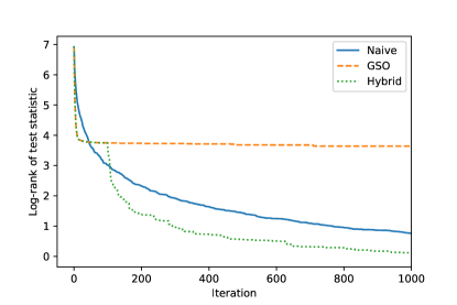
Figure 4: Comparison of the log-rank of the test statistic for each of the methodologies described in Section 1.3 when run on a semi-synthetic dataset created as described in Section 2.1 with $|\mathcal{X}|=47$ and $|\mathcal{Y}|=12$. The hybrid approach dominates both the naive and GSO approaches after a sufficient number of iterations.

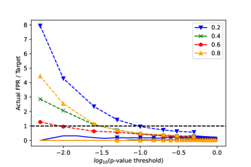
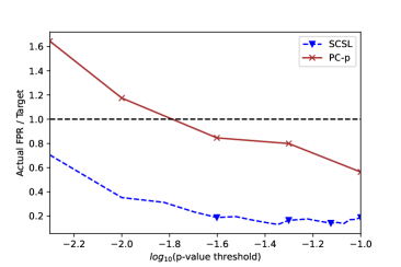
Figure 5: Left hand side shows the ratio of actual false positive rate to target rate on the PC-p algorithm (dashed) compared with the proposed methodology (solid) on semi-synthetic datasets generated with synthetic confounding and confoundedness parameter $p\in\{0.2,0.4,0.6,0.8\}$. Right hand side shows this ratio on a semi-synthetic dataset generated with real-world confounding which matches the complexity of the real dataset ($|\mathcal{X}|$ = 47 and $|\mathcal{Y}|$ = 23).

2.1 Semi-synthetic simulations with synthetic confounding

Causal structure in $\mathcal{Y}$ is the key challenge in our task, as illustrated in Figure 1. To evaluate the robustness of our method in the presence of different degrees of confoundedness, we construct a collection of semi-synthetic datasets where we stochastically control the degree of confounding, allowing us to stress test the methodology under adverse conditions.

Dataset construction

We take as input the actual datasets $\mathcal{D}_{\mathcal{X}}\in\{0,1\}^{n\times p}$ and generates a synthetic dataset for $\mathcal{Y}$ which we label $\tilde{\mathcal{D}}_{y}$. For each desired $Y_{k}$, we choose $K$ features in $\mathcal{X}$ and generate coefficients $\beta_{k}\in\mathbb{R}^{K}$ sampled from a $\mathcal{N}(2,1)$ distribution. We store the chosen features in $\mathcal{X}_{Y_{k}}^{\star}$ and denote $\mathcal{D}_{\mathcal{X},k,i}^{\star}\in\{0,1\}^{K}$ to be the corresponding realized values of the chosen features for the $i$th individual. We now proceed by generating the elements of $\tilde{\mathcal{D}}_{y}$ which we call $Y_{k,i}$ in a sequential way. For the first element, the likelihood is defined simply as $f_{Y_{1,i}}(\mathcal{D}_{\mathcal{X},k,i}^{\star}):=\frac{1}{1+\exp(-\beta_{k}^{T}\mathcal{D}_{\mathcal{X},k,i}^{\star})}$ and now $Y_{1,i}\sim\text{Ber}(f_{Y_{k,1}}(\mathcal{D}_{\mathcal{X},Y_{1},i}^{\star}))$ is generated.

For subsequent features $Y_{k,i}$, we also pick features $Y_{l}$ for $l<k$ with probability $p$ to contribute to the likelihood function. Denote $\mathcal{D}_{\mathcal{Y},Y_{k},i}^{\star}$ as vector containing the chosen $Y_{l}$ for an individual $i$ and the coefficients, again sampled from a $\mathcal{N}(2,1)$ distribution, as $\gamma_{k}$. Now, define the likelihood as $f_{Y_{k,i}}(\mathcal{D}_{\mathcal{X},k,i}^{\star},\mathcal{D}_{\mathcal{Y},k,i}^{\star}):=\frac{1}{1+\exp(-\beta_{k}^{T}\mathcal{D}_{\mathcal{X},k,i}^{\star}-\gamma_{k}^{T}\mathcal{D}_{\mathcal{Y},Y_{k},i}^{\star})}$ and again sample $Y_{k,i}\sim\text{Ber}\left(f_{Y_{k,i}}(\mathcal{D}_{\mathcal{X},k,i}^{\star},\mathcal{D}_{\mathcal{Y},Y_{k},i}^{\star})\right)$. One can think of $p$ as a confounding parameter which makes the causal learning problem more difficult by increasing the number of dependencies in the graph. This algorithm is described in detail in the Appendix.

Results

Figure 5 (left) shows the Type I error control for our method and the PC-p algorithm across four different levels of confoundedness ($p\in\{0.2,0.4,0.6,0.8\}$). Across all four levels, the PC-p algorithm inflates the Type I error rate, sometimes by as much as 8x the nominal level. We track the power of these methods in the Appendix. We note that the PC-p algorithm does have slightly higher power than our methodology in most settings but at the high price of not properly controlling the Type I error.

2.2 Semi-synthetic simulations with real-world confounding

In addition to having ground truth knowledge of outcomes, we may also want to maintain the dependence structure in $\mathcal{Y}$ in our simulations. To that end, we propose a data-generating scheme where the joint distribution of $\mathcal{X}$ and $\mathcal{Y}$ are preserved, but the conditional distribution $P(\mathcal{Y}\mid\mathcal{X})$ is synthetic.

Dataset construction

The algorithm takes the realized datasets $\mathcal{D}_{\mathcal{X}}\in\{0,1\}^{n\times p}$ and $\mathcal{D}_{\mathcal{Y}}\in\{0,1\}^{n\times m}$ and generates a synthetic data for $\mathcal{Y}$ which we denote $\tilde{\mathcal{D}}_{\mathcal{Y}}$. To do this, we sample $K$ features from $\mathcal{X}$ for every element of $\mathcal{Y}$. We let $\mathcal{X}_{k}^{\star}$ be the features of $\mathcal{X}$ chosen for a particular $Y_{k}$ and sample coefficients $\beta_{k}\in\mathbb{R}^{K}$ from a $\mathcal{N}(2,1)$ distribution.

Lettin $\mathcal{D}_{\mathcal{X},k,i}^{\star}\in\{0,1\}^{K}$ be the realized data points corresponding to the chosen features for the $i$th individual, we generate a logistic likelihood function $f_{Y_{k,i}}(\mathcal{D}_{\mathcal{X},k,i}^{\star}):=\frac{1}{1+\exp(-\beta_{k}^{T}\mathcal{D}_{\mathcal{X},k,i}^{\star})}$. An issue with using this likelihood function directly to generate the data is that the outcome dataset will no longer have the same dependence structure as the original. To circumvent this issue, we use the likelihood function to sample actual rows of $\mathcal{D}_{\mathcal{Y}}$. Specifically, we generate $\tilde{\mathcal{D}}_{\mathcal{Y},i}\sim\text{Cat}(\theta_{1},...,\theta_{n})$ where $\theta_{i}\propto\prod_{k}f_{Y_{k,i}}(\mathcal{D}_{\mathcal{X},k,i}^{\star})$. In other words, each row gets sampled in proportion to its overall likelihood under the assumed model. The procedure is described more explicitly in the Appendix.

$|\mathcal{X}|$	$|\mathcal{Y}|$	Power			Type I Error
		SCSL	FGES	BOSS	SCSL	FGES	BOSS
5	5	1.00	0.60	0.60	0.00	0.00	0.00
10	10	0.50	0.07	0.10	0.01	0.00	0.00
15	15	0.33	0.08	0.07	0.01	0.00	0.00
20	20	0.08	0.01	0.01	0.00	0.00	0.00
47	12	0.25	0.07	0.07	0.02	0.00	0.00
47	23	0.11	0.01	0.01	0.01	0.00	0.00

Table 1: Comparison of performance of SCSL to existing methods for large-scale causal discovery for datasets of different sizes. We note that power is significantly greater for the SCSL, although Type I error rates are similar.

Results

We first investigate how quickly the methods for optimizing the worst-case $p$-value described in Section 1.3 converge to the actual minimum, compared with the naive approach of randomly searching over the space in Figure 4. We see that the Gumbel-Softmax approach performs better than the naive approach at first, but then approaches an asymptote as it converges on a solution. The hybrid approach is able to dominate both approaches by allowing for both learning and exploration of the full combinatorial space. In this case, we manually choose to switch to sampling conditioning subsets without replacement at $200$ iterations, though in principle it may be possible to learn an optimal time to swap procedures from the data.

Figure 5 (right) shows the Type I error for SCSL and the PC-p algorithm on the generated data. The results mirror the synthetic confounding simulations, with the PC-p algorithm inflating the Type I error rate while SCSL achieves Type I error control. Discussions of the relative power between the two methods is again contained in the Appendix. Table 1 compares performance of SCSL (using $p$-value threshold $0.05$) with FGES and BOSS algorithms as the size of the constructed datasets scales up. We note type I error rates are similar, but the power of SCSL is significantly higher.

2.3 Results on real dataset

As a final step, we run the methodology on the real data. We stratify the dataset based on the primary tumor site location, and calculate $p$-values separately within each stratum to identify the secondary tumor location and gene combinations that are significant across different types of metastases. A rejection set is formed using the Benjamini-Hochberg (BH) [Benjamini and Hochberg, 1995] procedure with target FDR of 0.05 and is shown in Table 2. As a point of comparison, we also calculate the $p$-values for marginal tests of independence that the original paper used to identify connections. Figure 6 compares the marginal $p$-values used by the original paper with the causal $p$-values calculated through SCSL. Applying the BH procedure with the same target threshold results in $161$ rejections of marginal $p$-values. However, only $6$ of these $161$ remained in the causal rejection set.

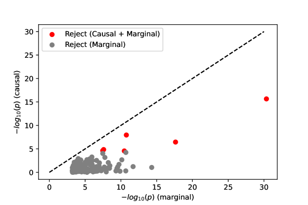
Figure 6: Plot of the $161$ discoveries rejected using the BH procedure with target FDR of $0.05$ on the marginal independence associations. Only $6$ of the discoveries were rejected when applying the BH procedure with the same target threshold on the causal $p$-values.

The causal mutations discovered have mechanistic evidence in the biology literature. For instance, CDH1 has been mechanistically investigated in breast cancer models of metastasis through its connection to asparagine [Knott et al., 2018]. Colon cancers are often treated with EGFR-inhibitors, which are ineffective in the presence of KRAS mutants which continue to activate the MAPK pathway, leading to eventual metastasis [Prenen et al., 2010]. TP53 mutations in certain pancreas cancers have been shown to increase fibrosis, enabling tumors to better evade the immune system and increasing metastatic potential [Maddalena et al., 2021]. While these mechanistic links between the primary site, gene, and general metastasis are known, the site-specific patterns have not been investigated. Thus, our causal testing results may provide valuable guidance to scientists and clinicians considering the utility of invasive patient monitoring.

			$p$-value
Primary	Gene	Secondary	Causal	Marginal
Breast	CDH1	Lung	$3.5\times 10^{-7}$	$2.3\times 10^{-18}$
Colon	KRAS	Lung	$1.4\times 10^{-5}$	$2.6\times 10^{-8}$
Liver	TERT	Liver	$2.3\times 10^{-5}$	$3.4\times 10^{-8}$
Lung	EGFR	CNS (Brain)	$2.8\times 10^{-5}$	$3.3\times 10^{-11}$
Pancreas	KRAS	Lymph	$2.2\times 10^{-16}$	$4.5\times 10^{-31}$
Pancreas	TP53	Lymph	$1.1\times 10^{-8}$	$1.7\times 10^{-11}$

Table 2: List of all genes and tumor combinations identified as significant at each primary site after forming a rejection set using the Benhamini-Hochberg procedure with target FDR of $0.05$, contrasted with the marginal $p$-values calculated using a Fisher exact test.

3 Conclusion

We introduced a new algorithm for causal discovery which drastically decreases the computational burden required to compute a $p$-value for a causal relationship between two nodes in a directed acyclic graph with temporally separated sets of variables. We tested this methodology on semi-synthetic data constructed from a recent study on somatic tumor mutations and metastatic potential for a panel of patients and found that the methodology successfully controlled Type I error and had reasonable power across datasets of differing levels of confoundedness. When run on the dataset of Nguyen et al. [2022] , interesting connections between metastases and genes are identified.

Several avenues for follow-up work exist. From a statistical perspective, the $p$-values generated from the procedure are conservative and power can potentially be improved through post-hoc adjustment to the $p$-values, for example through the use of Empirical Bayes methods [Efron, 2008]. From a computational perspective, more sophisticated probability models for finding the worst-case $p$-value could be used to search the combinatorial space. We also focused on the setting where a graph consists of only two groups of temporally separated nodes. It would be interesting to investigate how this methodology performs when adapted to datasets with several groups of nodes coming online at different times. Finally, although we have motivated our method from a metastasis dataset, the methodology is general and could be applied to a number of datasets in areas like genome-wide association studies.

Appendix A Algorithms for construction of semi-synthetic datasets

We include the pseudocode for construction of semi-synthetic datasets in Algorithm 2 and Algorithm 3 below.

Algorithm 2 Semi-synthetic dataset with synthetic confounding

  Data: $\mathcal{D}_{\mathcal{X}}\in\{0,1\}^{n\times p}$

  Shuffle rows of $\mathcal{D}_{\mathcal{X}}$ and store as $\tilde{\mathcal{D}}_{\mathcal{X}}$

  for $k=1$ to $|\mathcal{Y}|$ do

     Sample $K$ features from $\mathcal{X}$ and denote $\mathcal{X}_{k}^{\star}$ the features for a particular $Y_{k}$

     For each elements $Y_{k}\in\mathcal{S}_{2}$ with $l<k$, add $Y_{l}$ to $\mathcal{Y}_{Y_{k}}^{\star}$ with probability $p$.

     Sample coefficients $\beta_{k}\in\mathbb{R}^{K}$ for $\mathcal{X}_{Y_{k}}^{\star}$ (e.g., from a standard normal) and $\gamma_{k}\in\mathbb{R}^{K}$ for $\mathcal{Y}_{k}^{\star}$.

     Let $f_{Y_{k,i}}(\mathcal{D}_{\mathcal{X},k,i}^{\star},\mathcal{D}_{\mathcal{Y},k,i}^{\star}):=\frac{1}{1+\exp(-\beta_{k}^{T}\mathcal{D}_{\mathcal{X},k,i}^{\star}-\gamma_{k}^{T}\mathcal{D}_{\mathcal{Y},k,i}^{\star})}$ the likelihood associated with each response $Y_{k}$, where $\mathcal{D}_{\mathcal{X},k,i}^{\star}$ is the realized data corresponding to $\mathcal{X}_{k}^{\star}$ and $\mathcal{D}_{\mathcal{Y},k,i}^{\star}$ is a vector corresponding to the realized data for $\mathcal{Y}_{k}^{\star}$ for the $i$th individual in the dataset

     for row $i=1$ to $n$ do

        sample ${\tilde{\mathcal{D}}}_{Y_{k},i}\sim\text{Ber}(\theta_{i,k})$ with $\theta_{i,k}=f_{Y_{k,i}}(\mathcal{D}_{\mathcal{X},Y_{k},i}^{\star},\mathcal{D}_{\mathcal{Y},Y_{k},i}^{\star})$

     end for

  end for

  Return semi-synthetic data $\tilde{\mathcal{D}}_{\mathcal{X}}$ and $\tilde{\mathcal{D}}_{\mathcal{Y}}$

Algorithm 3 Semi-synthetic dataset with real-world confounding

  Input: Data: $\mathcal{D}_{\mathcal{X}}\in\{0,1\}^{n\times p}$ and $\mathcal{D}_{\mathcal{Y}}\in\{0,1\}^{n\times m}$,

  Shuffle rows of $\mathcal{D}_{\mathcal{X}}$ and store as $\tilde{\mathcal{D}}_{\mathcal{X}}$

  Shuffle rows of $\mathcal{D}_{\mathcal{Y}}$

  Sample $K$ features from $\mathcal{X}$ for each element of $\mathcal{Y}$ and denote $\mathcal{X}_{k}^{\star}$ the features for a particular $Y_{k}$

  Create likelihoods for the rows of $\mathcal{Y}$ from $\mathcal{X}^{\star}$ by

1. Sampling coefficients $\beta_{k}\in\mathbb{R}^{K}$ for $\mathcal{X}_{Y_{k}}^{\star}$ (e.g., from a standard normal)

2. Let $f_{Y_{k,i}}(\mathcal{D}_{\mathcal{X},k,i}^{\star}):=\frac{1}{1+\exp(-\beta_{k}^{T}\mathcal{D}_{\mathcal{X},k,i}^{\star})}$ be the likelihood associated with each response $Y_{k}$ and row $i$, where $\mathcal{D}_{\mathcal{X},k,i}^{\star}\in\{0,1\}^{K}$ are the realized data corresponding to $\mathcal{X}_{k}^{\star}$ for the $i$th individual in the dataset.

  for row $i=1$ to $n$ do

     sample ${\tilde{\mathcal{D}}}_{\mathcal{Y},i}\sim\text{Cat}(\theta_{1},\dots,\theta_{n})$ with $\theta_{i}\propto\prod_{k}f_{Y_{k,i}}(\mathcal{D}_{\mathcal{X},k,i}^{\star})$

  end for

  Return semi-synthetic data $\tilde{\mathcal{D}}_{\mathcal{X}}$ and $\tilde{\mathcal{D}}_{\mathcal{Y}}$

Appendix B Adjustments for continuous and mixed-value data

In Algorithm 4, we present a slightly augmented the methodology to train amortized predictive models to accommodate continuous valued data. The algorithm is largely the same as the one presented in the main paper, with the modification that both the masks $(B,M)$ and the interactions between the mask are inputs into the loss function. In the case that binary-valued data was used with $X_{j},Y_{k}\in\{-1,1\}$, then this was not necessary as the interactions would simply lead to the masked versions $\tilde{X}_{j},\tilde{Y}_{k}\in\{-1,0,1\}$. In the case of continuous or mixed valued data, however, there is a need to distinguish between data that is $0$ because it has been masked or data that is actually $0$.

To construct semi-synthetic datasets to test this dataset, Algorithm 3 and Algorithm 2 can be modified slightly by letting the likelihood functions correspond to a Gaussian distribution instead of a logistic response, and then sampling appropriately.

Algorithm 4 Amortized predictive model training for continuous response data

  Input: Data: $\mathcal{D}_{\mathcal{X}}\in\mathbb{R}^{n\times|\mathcal{X}|}$; $\mathcal{D}_{\mathcal{Y}}\in\mathbb{R}^{n\times|\mathcal{Y}|}$; $n_{ep}$ (number of epochs), $n_{batch}$ (batch size), $p$ (masking parameter), loss function $\ell\left(\theta,\mathcal{X},Y_{-k},Y_{k},B,M\right)$

  for $i=1$ to $n_{ep}$ do

     for $i=1$ to $[n/n_{batch}]$ do

        Draw $n_{batch}$ new samples

        Draw $B_{m}\sim\text{Ber}(p)$ for each $Y_{m}\in Y_{-k}$. Denote $B=\left(B_{1},\cdots,B_{k-1},B_{k+1},...,B_{|\mathcal{Y}|}\right)$.

        Draw $M\sim\text{Cat}(\mathcal{X},q)$ with equally-weighted probabilities

        Construct $\tilde{Y}_{-k}$ by taking each $Y^{i}_{m}$ in the sample and replacing with $\widetilde{Y}^{i}_{m}:=Y^{i}_{m}\times B_{m}$

        Construct $\tilde{\mathcal{X}}$ by taking each $X^{i}_{j}$ and replacing with $\widetilde{X}^{i}_{j}:=X^{i}_{j}\times\mathbbm{1}_{M\neq k}$

        Compute $\frac{\partial\ell(\tilde{\theta,\mathcal{X}},\tilde{Y}_{-k},Y_{k},B,M)}{\partial\theta}$

        $\theta\leftarrow\theta-\eta\frac{\partial\ell(\theta,\tilde{\mathcal{X}},\tilde{Y}_{-k},Y_{k},B,M)}{\partial\theta}$

     end for

  end for

Additional experimental results for data constructed in this manner are shown in Appendix E.

Appendix C Flowchart summarizing methodology

In Figure 7, we present a visual flowchart illustrating how to apply the methodology. Assumed inputs into this process are a method for computing $p$-values corresponding to conditional independence tests. For all of our experiments, we use amortization to efficiently compute the GCM test statistic for different conditioning subsets.

Figure 7: Flowchart illustrating the methodology. Nodes colored in blue represent $p$-values for the individual conditional independence tests corresponding to the “inner” null that $X_{j}\perp\!\!\!\perp Y_{k}|S,X_{-j}$. Nodes colored in yellow correspond to $p$-values testing the “outer” null that $X_{j}\rightarrow Y_{k}$ is absent.

Appendix D Technical exposition of Generalized Covariance Measure

We recall the details of the technical conditions described in Shah and Peters [2020] for completeness. We assume that the dataset consists of i.i.d. $n$ samples, with individual observations denoted $\{X_{j}^{i},Y_{k}^{i},S^{i},X_{-j}^{i}\}_{i=1}^{n}$. Let $\mathcal{P}_{0}$ denote the family of joint distributions corresponding to the null that $X_{j}\perp\!\!\!\perp Y_{k}|S,X_{-j}$.

We define $R_{i}=\left(X_{j}^{i}-\widehat{X}_{j}^{i}\right)\left(Y_{k}^{i}-\widehat{Y}_{k}^{i}\right)$ and the test statistic:

$$T^{(n)}=\frac{\sqrt{n}\cdot\frac{1}{n}\sum_{i=1}^{n}R_{i}}{\left(\frac{1}{n}\sum_{i=1}^{n}R_{i}^{2}-\left(\frac{1}{n}\sum_{r=1}^{n}R_{r}\right)^{2}\right)^{1/2}}.$$ (6)

We further denote $\epsilon_{j,P}:=X_{j}-\mathbb{E}_{P}[X_{j}|S,X_{-j}]$ and $\epsilon_{k,P}:=Y_{k}-\mathbb{E}_{P}[Y_{k}|S,X_{-j}]$.

Fact D.1 (Theorem 6 of Shah and Peters [2020]).

Define the following quantities:

$$A_{f}:=\frac{1}{n}\sum_{i=1}^{n}\left\{X_{j}^{i}-\widehat{X}_{j}^{i}\right\}^{2},\text{ }A_{g}:=\frac{1}{n}\sum_{i=1}^{n}\left\{Y_{k}^{i}-\widehat{Y}_{k}^{i}\right\}^{2},$$

$$B_{f}:=\frac{1}{n}\sum_{i=1}^{n}\left\{X_{j}^{i}-\widehat{X}_{j}^{i}\right\}^{2}\mathbb{E}_{P}\left(\epsilon_{j,P}^{2}|S,X_{-j}\right),\text{ and }B_{g}:=\frac{1}{n}\sum_{i=1}^{n}\left\{Y_{k}^{i}-\widehat{Y}_{k}^{i}\right\}^{2}\mathbb{E}_{P}\left(\epsilon_{k,P}^{2}|S,X_{-j}\right).$$

1. If for $P\in\mathcal{P}_{0}$, $A_{f}A_{g}=o(n^{-1})$, $B_{f}=o(1)$, $B_{g}=o(1)$, and $0\leq\mathbb{E}_{P}\left(\epsilon_{j,P}^{2}\epsilon_{k,P}^{2}\right)$, then $\sup_{t\in\mathbb{R}}|\mathbb{P}_{P}\left(T^{(n)}\leq t\right)-\Phi(t)|\rightarrow 0$.

2. Let $\mathcal{P}\subseteq\mathcal{P}_{0}$ denote the set of null distributions such that $A_{f}A_{g}=o(n^{-1})$, $B_{f}=o(1)$, $B_{g}=o(1)$, $\inf_{\mathcal{P}\in P}\mathbb{E}_{p}\mathbb{E}_{P}\left(\epsilon_{j}^{2}\epsilon_{k}^{2}\right)\geq c_{1}$, and $\sup_{\mathcal{P}\in P}\mathbb{E}_{p}\mathbb{E}_{P}\left(\epsilon_{j,P}^{2}\epsilon_{k,P}^{2}\right)\leq c_{2}$ for some $c_{1},c_{2}>0$. Then $\sup_{P\in\mathcal{P}}\sup_{t\in\mathbb{R}}|\mathbb{P}_{P}\left(T^{(n)}\leq t\right)-\Phi(t)|\rightarrow 0$.

Appendix E Additional experimental results

Additional results for each of the semi-synthetic simulations are shown in this section.

Additional information on alternative predictive modelling approaches

In addition to using a logistic regression to compute the underlying regression functions in the GCM test statistic, we also experimented with a multi-layer perceptron neural network with with $2$ hidden layers comprised of $200$ nodes in each layer and dropout regularization. The performance of this method is compared and contrasted with the logistic regression used in the main paper in Figure 8. Since the logistic regression had higher power, we focused on using it as a predictive model in the main paper.

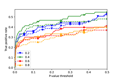
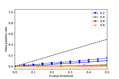
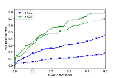
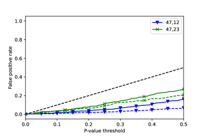
Figure 8: Type I error and Type II error rates for SCSL compared when logistic models (solid) are swapped out for a neural network (dashed). The top row shows results for the datasets with synthetic confounding while the bottom row shows results for datasets constructed with real confounding (note that the tuple $(a,b)$ in the legend indicates the number of variables contained in each node set with $|\mathcal{X}|=a$ and $|\mathcal{Y}|=b$ respectively). The performance across all methods is comparable, though we note the logistic model has higher power in general.

Additional results on power

As discussed in the results section, the PC-p algorithm does have higher power than SCSL, but this comes at the expense of Type I error control. This is a natural consequence of the fact that the PC-p algorithm draws an edge between two nodes based on a consideration set of CI tests that is a subset of the tests considered by SCSL. Since we use the same underlying CI test in our comparison of the methodologies, this necessitates that the PC-p algorithm will have strictly lower $p$-values than SCSL. Nonetheless, the decrease in power resulting from a move to this new methodology is not significant. We compare the power of the two methodologies side by side in Figure 9 for the same configuration of datasets discussed in the results section.

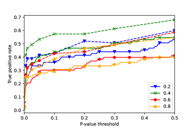
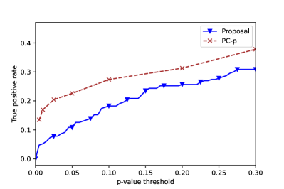
Figure 9: True positive rate for proposed methodology (solid) contrasted with PC-p method (dashed). Left-hand side shows the power for each of these methodologies run on datasets constructed by Algorithm 2 for the same sequence of confoundedness parameters discussed in the main paper with $p\in\{0.2,0.4,0.6,0.8\}$. Right-hand side shows the power for these two methods on the semi-synthetic dataset constructed with Algorithm 3.

Comparisons to procedures without frequentist error guarantees

Although the PC-p algorithm is the only existing method that aims at constructing $p$-values with frequentist error control, we also benchmark this procedure against approaches not aimed at controlling type I error that are implemented in the TETRAD project. The only two methods that scale reasonably to datasets of a similar size as the dataset of Nguyen et al. [2022] are Fast Greedy Equivalence Search (FGES) [Ramsey et al., 2017b] and the Best Order Score Search (BOSS) algorithm [Lam et al., 2022]. Results comparing these results to SCSL are shown in Table 3.

For other methods implemented in TETRAD, we benchmark using smaller semi-synthetic datasets constructed from Algorithm 3 and track how computation scales as the number of nodes in the graph increases in Figure 10. We note that the performance decreases drastically and computation time becomes intractable for graphs with more than $20$ nodes for all methods other than FGES and BOSS.

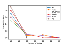
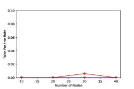
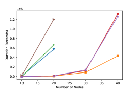
Figure 10: Perofrmance of causal discovery algorithms implemented in TETRAD for semi-synthetic datasets constructed from Algorithm 3. Performance of all methods decreases markedly for larger graphs. Entries are missing if computation time exceeds 36 hours for any method.

Algorithm	Type	$p$	$|\mathcal{S}_{1}|$	$|\mathcal{S}_{2}|$	TPR			FPR
					SCSL	FGES	BOSS	SCSL	FGES	BOSS
Algorithm 1	Discrete	0.3	5	5	0.40	0.40	0.40	0.07	0.00	0.00
Algorithm 1	Discrete	0.3	10	10	0.40	0.53	0.53	0.00	0.03	0.03
Algorithm 1	Discrete	0.3	15	15	0.38	0.55	0.62	0.01	0.08	0.01
Algorithm 1	Discrete	0.3	20	20	0.33	0.67	0.69	0.00	0.17	0.03
Algorithm 1	Discrete	0.2	47	15	0.33	0.49	0.52	0.01	0.03	0.02
Algorithm 1	Discrete	0.4	47	15	0.40	0.61	0.64	0.00	0.05	0.01
Algorithm 1	Discrete	0.6	47	15	0.29	0.53	0.60	0.00	0.05	0.01
Algorithm 1	Discrete	0.8	47	15	0.28	0.39	0.48	0.00	0.05	0.01
Algorithm 1	Continuous	0.1	47	15	0.80	0.95	0.95	0.00	0.01	0.00
Algorithm 1	Continuous	0.3	47	15	0.39	0.95	0.96	0.01	0.11	0.00
Algorithm 1	Continuous	0.5	47	15	0.13	0.88	0.99	0.00	0.30	0.00
Algorithm 1	Continuous	0.7	47	15	0.27	0.95	0.96	0.02	0.25	0.00
Algorithm 2	Discrete		5	5	1.00	0.60	0.60	0.00	0.00	0.00
Algorithm 2	Discrete		10	10	0.50	0.07	0.10	0.01	0.00	0.00
Algorithm 2	Discrete		15	15	0.33	0.08	0.07	0.01	0.00	0.00
Algorithm 2	Discrete		20	20	0.08	0.01	0.01	0.00	0.00	0.00
Algorithm 2	Discrete		47	12	0.25	0.07	0.07	0.02	0.00	0.00
Algorithm 2	Discrete		47	23	0.11	0.01	0.01	0.01	0.00	0.00

Table 3: Comparison between FGES and BOSS algorithms for causal discovery with SCSL across different configurations of semi-synthetic datasets constructed using Algorithm 2 andAlgorithm 3. Since SCSL outputs a $p$-value for each edge rather than a binary decision, a $p$-value threshold of $0.05$ is used to compare to the other two algorithms. No algorithm appears to dominate the others in all settings, but we note that FGES and BOSS both have considerable difficulty in detecting edges in the presensce of real-world confounding as defined in Algorithm 3.

References

- Annadani et al. [2021] Yashas Annadani, Jonas Rothfuss, Alexandre Lacoste, Nino Scherrer, Anirudh Goyal, Yoshua Bengio, and Stefan Bauer. Variational causal networks: Approximate bayesian inference over causal structures. arXiv preprint arXiv:2106.07635, 2021.
- Aragam and Zhou [2015] Bryon Aragam and Qing Zhou. Concave penalized estimation of sparse gaussian bayesian networks. J. Mach. Learn. Res., 16(1), 2015.
- Benjamini and Hochberg [1995] Yoav Benjamini and Yosef Hochberg. Controlling the false discovery rate: A practical and powerful approach to multiple testing. J. of the Royal Statistical Society. Series B (Methodological), 57(1):289–300, 1995.
- Brastianos et al. [2015] Priscilla K Brastianos, Scott L Carter, Sandro Santagata, Daniel P Cahill, Amaro Taylor-Weiner, Robert T Jones, Eliezer M Van Allen, Michael S Lawrence, Peleg M Horowitz, Kristian Cibulskis, et al. Genomic characterization of brain metastases reveals branched evolution and potential therapeutic targets. Cancer Discovery, 5(11):1164–1177, 2015.
- Brown et al. [2017] David Brown, Dominiek Smeets, Borbála Székely, Denis Larsimont, A Marcell Szász, Pierre-Yves Adnet, Françoise Rothé, Ghizlane Rouas, Zsófia I Nagy, Zsófia Faragó, et al. Phylogenetic analysis of metastatic progression in breast cancer using somatic mutations and copy number aberrations. Nature Communications, 8(1):1–13, 2017.
- Candes et al. [2016] Emmanuel Candes, Yingying Fan, Lucas Janson, and Jinchi Lv. Panning for Gold: Model-free Knockoffs for High-dimensional Controlled Variable Selection. J. of the Royal Statistical Society: Series B (Statistical Methodology), 80, 10 2016.
- Cheng et al. [2015] Donavan T Cheng, Talia N Mitchell, Ahmet Zehir, Ronak H Shah, Ryma Benayed, Aijazuddin Syed, Raghu Chandramohan, Zhen Yu Liu, Helen H Won, Sasinya N Scott, et al. Memorial Sloan Kettering-Integrated Mutation Profiling of Actionable Cancer Targets (MSK-IMPACT): a hybridization capture-based next-generation sequencing clinical assay for solid tumor molecular oncology. The J. of Molecular Diagnostics, 17(3):251–264, 2015.
- Chickering [2003] David Maxwell Chickering. Optimal structure identification with greedy search. J. Mach. Learn. Res., 3:507–554, 2003.
- Cundy et al. [2021a] Chris Cundy, Aditya Grover, and Stefano Ermon. BCD nets: Scalable variational approaches for bayesian causal discovery. In Advances in Neural Information Processing Systems, volume 34, pages 7095–7110, 2021a.
- Cundy et al. [2021b] Chris Cundy, Aditya Grover, and Stefano Ermon. BCD nets: Scalable variational approaches for bayesian causal discovery. In Advances in Neural Information Processing Systems, 2021b.
- D and Heckerman [1997] Maxwell D and David Heckerman. Efficient approximations for the marginal likelihood of bayesian networks with hidden variables. Machine Learning, 29:181–212, 11 1997.
- Efron [2008] Bradley Efron. Microarrays, Empirical Bayes and the Two-Groups Model. Statistical Science, 23(1):1 – 22, 2008.
- Fu and Zhou [2013] Fei Fu and Qing Zhou. Learning sparse causal gaussian networks with experimental intervention: Regularization and coordinate descent. J. of the American Statistical Association, 108(501):288–300, 2013.
- Goeman and Solari [2014] Jelle J. Goeman and Aldo Solari. Multiple hypothesis testing in genomics. Statistics in Medicine, 33(11):1946–1978, 2014.
- Heckerman et al. [1995] David Heckerman, Dan Geiger, and David Chickering. Learning bayesian networks: The combination of knowledge and statistical data. Machine Learning, 20:197–243, 1995.
- Jang et al. [2017] Eric Jang, Shixiang Gu, and Ben Poole. Categorical reparameterization with gumbel-softmax. In 5th International Conference on Learning Representations, ICLR 2017, 2017.
- Knott et al. [2018] Simon R. V. Knott, Elvin Wagenblast, Showkhin Khan, Sun Y. Kim, Mar Soto, Michel Wagner, Marc-Olivier Turgeon, Lisa Fish, Nicolas Erard, Annika L. Gable, Ashley R. Maceli, Steffen Dickopf, Evangelia K. Papachristou, Clive S. D’Santos, Lisa A. Carey, John E. Wilkinson, J. Chuck Harrell, Charles M. Perou, Hani Goodarzi, George Poulogiannis, and Gregory J. Hannon. Asparagine bioavailability governs metastasis in a model of breast cancer. Nature, 554(7692):378–381, 2018.
- Lam et al. [2022] Wai-Yin Lam, Bryan Andrews, and Joseph Ramsey. Greedy relaxations of the sparsest permutation algorithm. In James Cussens and Kun Zhang, editors, Proceedings of the Thirty-Eighth Conference on Uncertainty in Artificial Intelligence, volume 180 of Proceedings of Machine Learning Research, pages 1052–1062. PMLR, 01–05 Aug 2022. URL https://proceedings.mlr.press/v180/lam22a.html.
- Liu et al. [2021] Molei Liu, Eugene Katsevich, Lucas Janson, and Aaditya Ramdas. Fast and powerful conditional randomization testing via distillation. Biometrika, 109(2):277–293, 07 2021.
- Maddalena et al. [2021] Martino Maddalena, Giuseppe Mallel, Nishanth Belugali Nataraj, Michal Shreberk-Shaked, Ori Hassin, Saptaparna Mukherjee, Sharathchandra Arandkar, Ron Rotkopf, Abby Kapsack, Giuseppina Lambiase, Bianca Pellegrino, Eyal Ben-Isaac, Ofra Golani, Yoseph Addadi, Emma Hajaj, Raya Eilam, Ravid Straussman, Yosef Yarden, Michal Lotem, and Moshe Oren. Tp53 missense mutations in pdac are associated with enhanced fibrosis and an immunosuppressive microenvironment. Proceedings of the National Academy of Sciences, 118(23):e2025631118, 2021.
- Nguyen et al. [2022] Bastien Nguyen, Christopher Fong, Anisha Luthra, Shaleigh A. Smith, Renzo G. DiNatale, Subhiksha Nandakumar, Henry Walch, Walid K. Chatila, Ramyasree Madupuri, Ritika Kundra, Craig M. Bielski, Brooke Mastrogiacomo, Mark T.A. Donoghue, Adrienne Boire, Sarat Chandarlapaty, Karuna Ganesh, James J. Harding, Christine A. Iacobuzio-Donahue, Pedram Razavi, Ed Reznik, Charles M. Rudin, Dmitriy Zamarin, Wassim Abida, Ghassan K. Abou-Alfa, Carol Aghajanian, Andrea Cercek, Ping Chi, Darren Feldman, Alan L. Ho, Gopakumar Iyer, Yelena Y. Janjigian, Michael Morris, Robert J. Motzer, Eileen M. O’Reilly, Michael A. Postow, Nitya P. Raj, Gregory J. Riely, Mark E. Robson, Jonathan E. Rosenberg, Anton Safonov, Alexander N. Shoushtari, William Tap, Min Yuen Teo, Anna M. Varghese, Martin Voss, Rona Yaeger, Marjorie G. Zauderer, Nadeem Abu-Rustum, Julio Garcia-Aguilar, Bernard Bochner, Abraham Hakimi, William R. Jarnagin, David R. Jones, Daniela Molena, Luc Morris, Eric Rios-Doria, Paul Russo, Samuel Singer, Vivian E. Strong, Debyani Chakravarty, Lora H. Ellenson, Anuradha Gopalan, Jorge S. Reis-Filho, Britta Weigelt, Marc Ladanyi, Mithat Gonen, Sohrab P. Shah, Joan Massague, Jianjiong Gao, Ahmet Zehir, Michael F. Berger, David B. Solit, Samuel F. Bakhoum, Francisco Sanchez-Vega, and Nikolaus Schultz. Genomic characterization of metastatic patterns from prospective clinical sequencing of 25,000 patients. Cell, 185(3):563–575, 2022.
- Ogburn et al. [2022] Elizabeth L. Ogburn, Oleg Sofrygin, Iván Díaz, and Mark J. van der Laan. Causal inference for social network data. J. of the American Statistical Association, 0(0):1–15, 2022.
- Paschos et al. [2009] Konstantinos A Paschos, David Canovas, and Nigel C Bird. The role of cell adhesion molecules in the progression of colorectal cancer and the development of liver metastasis. Cellular Signalling, 21(5):665–674, 2009.
- Peters et al. [2016] Jonas Peters, Peter Bühlmann, and Nicolai Meinshausen. Causal Inference by using Invariant Prediction: Identification and Confidence Intervals. Journal of the Royal Statistical Society Series B: Statistical Methodology, 78(5):947–1012, 10 2016. ISSN 1369-7412. doi: 10.1111/rssb.12167. URL https://doi.org/10.1111/rssb.12167.
- Prenen et al. [2010] Hans Prenen, Sabine Tejpar, and Eric Van Cutsem. New strategies for treatment of KRAS mutant metastatic colorectal cancer. Clinical Cancer Research, 16(11):2921–2926, 2010.
- Ramsey et al. [2006] Joseph Ramsey, Peter Spirtes, and Jiji Zhang. Adjacency-faithfulness and conservative causal inference. In Proceedings of the Twenty-Second Conference on Uncertainty in Artificial Intelligence, page 401–408, 2006.
- Ramsey et al. [2017a] Joseph Ramsey, Madelyn Glymour, Ruben Sanchez-Romero, and Clark Glymour. A million variables and more: the fast greedy equivalence search algorithm for learning high-dimensional graphical causal models, with an application to functional magnetic resonance images. International J. of Data Science and Analytics, 3:121–129, 2017a.
- Ramsey et al. [2017b] Joseph Ramsey, Madelyn Glymour, Ruben sanchez romero, and Clark Glymour. A million variables and more: the fast greedy equivalence search algorithm for learning high-dimensional graphical causal models, with an application to functional magnetic resonance images. International Journal of Data Science and Analytics, 3, 03 2017b. doi: 10.1007/s41060-016-0032-z.
- Raskutti and Uhler [2018] Garvesh Raskutti and Caroline Uhler. Learning directed acyclic graph models based on sparsest permutations. Stat, 7(1):e183, 2018. doi: https://doi.org/10.1002/sta4.183. URL https://onlinelibrary.wiley.com/doi/abs/10.1002/sta4.183. e183 sta4.183.
- Shah and Peters [2020] Rajen Shah and Jonas Peters. The hardness of conditional independence testing and the generalised covariance measure. Annals of Statistics, 48, 04 2020.
- Shimizu et al. [2011] Shohei Shimizu, Takanori Inazumi, Yasuhiro Sogawa, Aapo Hyvärinen, Yoshinobu Kawahara, Takashi Washio, Patrik O. Hoyer, and Kenneth Bollen. DirectLiNGAM: A direct method for learning a linear non-gaussian structural equation model. J. Mach. Learn. Res., 12:1225–1248, 2011.
- Solus et al. [2017] Liam Solus, Yf Wang, Lenka Matejovicova, and Caroline Uhler. Consistency guarantees for permutation-based causal inference algorithms. Biometrika, 108, 02 2017. doi: 10.1093/biomet/asaa104.
- Spirtes [2001] Peter Spirtes. An anytime algorithm for causal inference. In Proceedings of the Eighth International Workshop on Artificial Intelligence and Statistics, volume R3 of Proceedings of Machine Learning Research, pages 278–285, 2001.
- Spirtes et al. [2000] Peter Spirtes, Clark N Glymour, Richard Scheines, and David Heckerman. Causation, prediction, and search. MIT press, 2000.
- Strobl et al. [2019] Eric V. Strobl, Peter L. Spirtes, and Shyam Visweswaran. Estimating and controlling the false discovery rate of the pc algorithm using edge-specific p-values. 10(5), 2019.
- Tansey et al. [2022] Wesley Tansey, Victor Veitch, Haoran Zhang, Raul Rabadan, and David M. Blei. The holdout randomization test for feature selection in black box models. J. of Computational and Graphical Statistics, 31(1):151–162, 2022.
- Tennant et al. [2020] Peter W G Tennant, Eleanor J Murray, Kellyn F Arnold, Laurie Berrie, Matthew P Fox, Sarah C Gadd, Wendy J Harrison, Claire Keeble, Lynsie R Ranker, Johannes Textor, Georgia D Tomova, Mark S Gilthorpe, and George T H Ellison. Use of directed acyclic graphs (DAGs) to identify confounders in applied health research: review and recommendations. International J. of Epidemiology, 50(2):620–632, 12 2020.
- Zheng et al. [2018] Xun Zheng, Bryon Aragam, Pradeep Ravikumar, and Eric P. Xing. DAGs with NO TEARS: Continuous Optimization for Structure Learning. In Advances in Neural Information Processing Systems, 2018.