Inferring entropy production from time-dependent moments
Abstract
Measuring entropy production of a system directly from the experimental data is highly desirable since it gives a quantifiable measure of the time-irreversibility for non-equilibrium systems and can be used as a cost function to optimize the performance of the system. Although numerous methods are available to infer the entropy production of stationary systems, there are only a limited number of methods that have been proposed for time-dependent systems and, to the best of our knowledge, none of these methods have been applied to experimental systems. Herein, we develop a general non-invasive methodology to infer a lower bound on the mean total entropy production for arbitrary time-dependent continuous-state Markov systems in terms of the moments of the underlying state variables. The method gives surprisingly accurate estimates for the entropy production, both for theoretical toy models and for experimental bit erasure, even with a very limited amount of experimental data.
I Introduction
In the last two decades, the framework of stochastic thermodynamics has enabled us to give thermodynamic interpretation to mesoscopic systems that are driven arbitrarily far from equilibrium [1]. Using the assumption of local detailed balance and a time scale separation between the system and its environment, one can define thermodynamic quantities such as heat, work and entropy production for general Markov systems [2, 3]. General results such as fluctuation theorems and thermodynamic uncertainty relations have been proposed and verified experimentally [4, 5, 6, 7, 8, 9, 10, 11, 12, 13, 14]. A fundamental quantity in stochastic thermodynamics is the entropy production [1, 2]. Indeed, minimising entropy production is an important problem in several applications, such as heat engines [15], information processing [16] and biological systems [17, 18]. Furthermore, it provides information and places bounds on the dynamics of the system in the form of the thermodynamic speed limits [20, 22, 23, 19, 25, 21, 24, 26, 27] and the dissipation-time uncertainty relation [28, 29, 30, 31]. Meanwhile measuring entropy production experimentally is difficult since one needs extensive knowledge about the details of the system, requiring a large amount of data.
Over the last couple of years, several methods have been developed to infer entropy production and other thermodynamic quantities in a model-free way or with limited information about the underlying system [32]. These techniques involve estimating entropy production using some experimentally accessible quantities. This includes methods based on thermodynamic bounds, such as the thermodynamic uncertainty relation [33, 34, 35], inference schemes based on the measured waiting-time distribution [36, 37, 38, 39, 40], and methods based on ignoring higher-order interactions [41, 42]. However, most of these methods focus only on steady-state systems and do not work for time-dependent processes [43, 44, 45, 46, 47]. Nonetheless, time-dependent dynamics plays a crucial role in many systems. One can for example think about nano-electronic processes, such as bit erasure or AC-driven circuits, but also in biological systems, where oscillations in, e.g., metabolic rates or transcription factors, effectively lead to time-dependent driving [50, 51, 48, 49]. There are few methods to infer entropy production for time-dependent systems [11, 52, 12, 53, 54, 55], and it is often challenging to apply them to experimental data. For instance, thermodynamic bound-based methods require the measurement of quantities such as response functions [11, 52] or time-inverted dynamics [12], which require an invasive treatment of the system. Another interesting method combines machine learning with a variational approach [54]. This method does however require a large amount of experimental data and a high temporal resolution. This might also be the reason why, to the best of our knowledge, no experimental studies exist on the inference of entropy production under time-dependent driving.
This paper aims to address these issues by deriving a general lower bound on the mean of the total entropy produced for continuous-state time-dependent Markov systems in terms of the time-dependent moments of the underlying state variables. The method gives an analytic lower bound for the entropy production if one only focuses on the first two moments and reduces to a numerical scheme if higher moments are taken into account. The scheme also gives the optimal force field that minimizes the entropy production for the given time-dependent moments. After presenting the theoretical calculations and applications to analytically solvable models, we will test our method in an experimental scenario involving the erasure of computational bits [50]. The method works surprisingly well for all examples, even when only the first two moments are taken into account and with a very limited amount of data ( trajectories).
In the following, we first recall some known results from stochastic thermodynamics in Section II, which will then be used to derive bounds first for one-dimensional systems in Section III and subsequently in general -dimensional systems in Section IV. Subsequently, we apply our method to the theoretical toy examples in Section V and to the experimental trajectories associated with erasure operation of computational bits in Section VI. Finally, we conclude in Section VII.
II Stochastic thermodynamics
We consider a -dimensional stochastic system whose state at time is denoted by a variable . The system experiences a time-dependent force field and is in contact with a thermal reservoir at constant temperature . The stochastic variable evolves according to an overdamped Langevin equation
| (1) |
is the Boltzmann constant and represents the Gaussian white noise with and , with being the diffusion matrix. One can also write the Fokker-Planck equation associated with the probability distribution as
| (2) |
with being the probability flux given by
| (3) |
This Fokker-Planck equation arises in a broad class of physical systems like colloidal particles [56], electronic circuits [51] and spin systems [57]. Stochastic thermodynamics dictates that the mean total entropy produced when the system runs up to time is given by [2]
| (4) |
Although this formula, in principle, allows one to calculate the entropy production of any system described by a Fokker-Planck equation, one would need the force field and probability distribution at each point in space and time. This is generally not feasible in experimental set-ups.
In this paper, our aim is to develop a technique that gives information about the total entropy production in terms of experimentally accessible quantities. Using methods from the optimal transport theory [59, 58, 20], we will derive a non-trivial lower bound on completely in terms of the moments of . This means, we can infer an estimate for simply by measuring the first few moments.
III Bound for one-dimensional systems
Let us first look at the one-dimensional case and denote the -th moment of by . Throughout this paper, we assume that these moments are finite for the entire duration of the protocol. We will first look at the case where one only has access to the first two moments and , as the resulting estimate for the entropy production has a rather simple and elegant expression. Subsequently we will turn to the more general case. Throughout the main text, we will assume that the diffusion coefficient is constant, but the results can be extended to spatially-dependent diffusion coefficients as discussed in Appendix E
III.1 First two moments
Our central goal is to obtain a lower bound on , constrained on the known time-dependent moments. This can be done by minimizing the following action:
| (5) |
with respect to the driving protocol, . We have introduced four Lagrange multipliers, two of which, namely and associated with fixing of first two moments at the final time and the other two, and at the intermediate times. In the action, we have included the contribution of moments at the final time separately, as dictated by the Pontryagin’s Maximum Principle [60]
Minimizing the action with respect to seems very complicated, due to the non-trivial dependence of on in Eq. (2). To circumvent this problem, we use methods from the optimal transport theory and introduce a coordinate transformation as [58]
| (6) |
and overdot indicating the time derivative. Mathematically, this coordinate transformation is equivalent to changing from Eulerian to Lagrangian description in fluid mechanics. It has also been used to derive other thermodynamic bounds such as the thermodynamic speed limit [20]. Using this equivalence, one can show that [61]
| (7) | ||||
| (8) |
for any test function and initial probability distribution . Plugging , we get
| (9) |
On the other hand, putting in Eq. (8), we obtain
| (10) |
Similarly, the moments and their time-derivatives are given by
| (11) | ||||
| (12) |
We can also write the force-field in terms of by using Eqs. (3) and (6). Hence we can calculate various quantities such as probability distribution, mean total dissipation, and force field utilizing . In fact, it turns out that is uniquely determined for a given force-field. Using the relations in Eqs. (7) and (8), we can reformulate the optimisation of the action in Eq. (5) with respect to as an optimisation problem in . Meanwhile one can rewrite as
| (13) |
For a small change , the total change in action is
| (14) |
For the optimal protocol, this small change has to vanish. Vanishing of the first term on the right hand side for arbitrary gives the Euler-Lagrangian equation
| (15) |
Let us now analyse the other two terms. Recall that for all possible paths , optimisation is being performed with the fixed initial condition [see Eq. (6)]. Consequently, we have which ensures that the second term on the right hand side of Eq. (14) goes to zero. On the other hand, the value of at the final time can be different for different paths which gives . For the second line to vanish, we must then have the pre-factor associated with equal to zero. Thus, we get two boundary conditions in time
| (16) | ||||
| (17) |
Observe that the first equation clearly demonstrates the importance of incorporating the terms at the final time in the action described in Eq. (5). If these terms are omitted, we would obtain , which according to Eq. (12) suggests that the time derivative of moments at the final time is zero. However, this is not true. To get consistent boundary condition, it is necessary for and to be non-zero.
Proceeding to solve Eq. (15), one can verify that
| (18) |
where and are functions that are related to the Lagrange multipliers and . To see this relation, one can take the time derivative in Eq. (18) and compare it with the Euler-Lagrange equation (15) to obtain
| (19) |
Let us now compute these -functions. For this, we use the solution of in in Eq. (12) for and . This yields
| (20) |
One can then use Eq. (10) to show that satisfies the bound
| (21) |
where is the variance of and is the bound on the mean total entropy produced with first and second moments fixed. Eq. (21) is one of the central results of our paper. It gives a lower bound on the mean total entropy dissipated completely in terms of the first moment and variance.
In our analysis, we have focused on minimizing the mean total entropy generated up to time with respect to the force field. However, an alternative approach involves minimizing the entropy production rate at each intermediate time, as opposed to the total entropy production, but, in Appendix A, we show that this approach generally leads to sub-optimal protocols and therefore no longer gives a bound on the total entropy production.
III.2 Optimal protocol with first two moments
Having obtained a lower bound for the entropy production, it is a natural question to ask for which protocols this bound is saturated. To answer that question, we first turn to the flux that gives rise to this optimal value. For this, we use Eqs. (6) and (18) and obtain
| (22) |
with -functions given in Eq. (20). One can verify that this equation is always satisfied for Gaussian processes. This is shown in Appendix B.
Next, we turn to the probability distribution associated with the optimal dissipation. For this, one needs the form of which follows from Eq. (18)
| (23) | ||||
| with | (24) |
Plugging this in Eq. (9), we obtain the distribution as
| (25) |
which then gives the optimal force-field as
| (26) |
We see that the optimal protocol comprises solely of a conservative force field with the associated energy landscape characterized by two components: the first two terms correspond to a time-dependent harmonic oscillator, whereas the last term has the same shape as the equilibrium landscape associated with the initial state. Furthermore, from Eq. (25), we also observe that this optimal protocol preserves the shape of the initial probability distribution. A similar result was also recently observed in the context of the precision-dissipation trade-off relation for driven stochastic systems [62].
III.3 Fixing first moments
So far, we have derived a bound on based only on the knowledge of first two moments. We will now generalise this for arbitrary number of moments. Consider the general situation where the first moments of the variable are given. Our goal is to optimise the action
| (27) |
with respect to . Once again, - functions are the Lagrange multipliers for moments with contribution at the final time included separately. As done before in Eq. (6), we introduce the new coordinate , and rewrite the action in terms of this map
For a small change , the total change in action is
| (28) |
which vanishes for the optimal path. Following the same line of reasoning as Section III.1, we then obtain the Euler-Lagrange equation
| (29) |
with two boundary conditions
| (30) | ||||
| (31) |
However, we still need to compute functions and with in order to completely specify the boundary conditions. To calculate -functions, we use Eq. (12) and obtain
| (32) |
On the other hand, for -functions, we use the second derivative of moments and obtain
| (33) | ||||
| (34) |
Both Eqs. (32) and (33) hold for all positive integer values of . Solving this gives all and functions in terms of , and , .
Once Eq. (29) is solved, the bound on mean total entropy dissipated can then be written as
| (35) |
Unfortunately, we could not obtain an analytic expression for Eq. (29) due to the presence of higher-order moments and , which are not a priori known. Instead, we will focus on numerically integrating Eq. (29). One can use the value of to calculate the higher-order moments and therefore the ’s in Eq. (33), which in turn can be used to obtain . Finally, one can make sure that the boundary condition, Eq. (30), is satisfied through a shooting method.
IV Bound in higher dimensions
Having developed a general methodology in one dimension, we now extend these ideas to higher dimensional systems with state variables . Herein again, our aim is to obtain a bound on with information about moments, including mixed moments.
IV.1 First two moments
As before, let us first introduce the notation
| (36) | |||
| (37) |
for first two (mixed) moments of variables. Once again, this is a constrained optimisation problem and we introduce the following action functional
| (38) |
where functions , , and all stand for Lagrange multipliers associated with given constraints. Further carrying out this optimisation is challenging since distribution depends non-trivially on the force-field . We, therefore, introduce a -dimensional coordinate
| (39) |
and rewrite completely in terms of . We then follow same steps as done in Section III.1 but in higher dimensional setting. Since this is a straightforward generalisation, we relegate this calculation to Appendix C and present only the final results here. For the optimal protocol, we find
| (40) |
with functions related to the Lagrange multipliers , via Eq. (125). Furthermore, in Appendix C, we show that functions are the solutions of a set of linear equations:
| (41) |
where and are two matrices with elements and respectively. Notice that the elements of comprise only of variance and covariance which are known. Therefore, the matrix is fully known at all times.
To solve Eq. (41), we note that is a symmetric matrix and thus, there exists an orthogonal matrix such that
| (42) |
where is a diagonal matrix whose elements correspond to the (positive) eigenvalues of . can be constructed using eigenvectors of and it satisfies the orthogonality condition . Combining the transformation Eq. (42) with Eq. (41), we obtain
| (43) | ||||
| (44) |
This relation enables us to write in Eq. (40) as
| (45) |
Finally, plugging this in the formula
| (46) |
we obtain the bound in general dimensions as
| (47) |
where the elements of matrix are fully given in terms of in Eq. (44) which in turn depends on the variance and covariance of . Eq. (47) represents a general bound on the mean entropy production in higher dimensions. For the two-dimensional case, we obtain an explicit expression (see Appendix C.1)
| (48) |
The bound is equal to the sum of two one dimensional bounds in Eq. (21) corresponding to two coordinates and plus a part that arises due to the cross-correlation between them. In absence of this cross-correlation , Eq. (48) correctly reduces to the sum of two separate one dimensional bounds.
IV.2 Optimal protocols with first two moments
Let us now look at the flux and the distribution associated with this optimal dissipation. For this, we first rewrite Eq. (40) in vectorial form as
| (49) |
and solve it to obtain the solution as
| (50) |
Here stands for the time-ordered exponential and is given by
| (51) |
with defined in Eq. (44) and corresponding to the time-ordering operator. Finally, substituting the solution from Eq. (50) in Eqs. (39) and (117), we obtain the optimal flux and optimal distribution as
| (52) | ||||
| (53) |
Now the optimal force-field follows straightforwardly from Eq. (3) as
| (54) |
To sum up, we have derived a lower bound to the total dissipation in general dimensions just from the information about first two moments. Together with this, we also calculated the force-field that gives rise to this optimal value. In what follows, we consider the most general case where we know the first- (mixed) moments of the state variable .
IV.3 Fixing first moments in general dimensions
Let us define a general mixed moment as
| (55) |
where and for all . For and , Eq. (55) reduces to first two moments in Eq. (37). Here, we are interested in the general case for which we consider the following action
| (56) |
In conjunction to the previous sections, we again recast this action in terms of defined in Eq. (39) as
| (57) | ||||
Optimising this action in the same way as before, we obtain the Euler-Lagrange equation
| (58) |
along with the boundary conditions
| (59) | ||||
| (60) |
The Lagrange multipliers and can be computed using time-derivatives of the (mixed) moments as
V Theoretical examples
We now test our framework on two analytically solvable toy models. The first one consists of a one dimensional free diffusion model with initial position drawn from the distribution . This example will demonstrate how our method becomes more accurate when we incorporate knowledge of higher moments. The second example involves two-dimensional diffusion in a moving trap, serving as an illustration of our method’s applicability in higher dimensions.
V.1 Free diffusion with
We first consider a freely diffusing particle in one dimension
| (64) |
This example serves two purposes: First, we can obtain the exact expression of which enables us to rigorously compare the bounds derived above with their exact counterpart. Second, we discuss the intricacies that arise when we fix more than first two moments. To begin with, the position distribution is given by
| (65) |
Since no external force acts on the system, the total entropy produced will be equal to the total entropy change of the system. Therefore, the mean reads
| (66) |
We emphasize that Eqs. (65) and (66) are exact results and do not involve any approximation.
Let us now analyse how our bound compares with this exact value. The first four moments of the position are given by
| (67) | |||
| (68) | |||
| (69) |
Combining this with Eq. (35), shows that the dissipation bound for the first two moments reads
| (70) | ||||
| (71) |
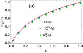
As illustrated in Figure 1(a), this bound , although not exact, is still remarkably close to the exact value in Eq. (66). This is somewhat surprising as one can show that the force field that saturates the bound is given by
| (72) |
which is significantly different from the force field associated with free relaxation ().
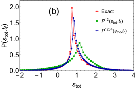
Going beyond mean, we have also plotted the full probability distribution of total dissipation in Figure 1(b). To do this, we evolve the particle with the optimal force-field in Eq. (72) starting from the position drawn from the distribution in Eq. (64). For different trajectories thus obtained, we measure the total entropy produced and construct the probability distribution out of them. Figure 1(b) shows the result. Here, we see deviation from the exact result indicating that fixing first two moments only does not give a very good approximation of dissipation beyond its average value. To improve this, we instead fix the first four moments of position and carry out this analysis.
One can wonder whether it is possible to get an even better estimate by taking into account the first four moments. To check this, we will now proceed by solving the Euler-Lagrange equation (29) numerically for . Since, this is a second-order differential equation, we need two boundary conditions in time. One of them is Eq. (31) which gives . However, the other one in Eq. (30) gives a condition at final time which is difficult to implement numerically. For this, we use the following trick. We expand the initial as
| (73) |
where we typically choose . The coefficients are free to vary but must give the correct time derivative of first four moments in Eqs. (67)-(69). We then assign a cost function as
| (74) |
Observe that the cost function vanishes if the boundary condition (30) is satisfied. Starting from and in Eq. (73), we solve the Euler-Lagrange equation (29) numerically and measure the cost function at the final time. We then perform a multi-dimensional gradient descent in -parameters to minimise . Eventually, we obtain the numerical form of the optimal map .
Using this map, we then obtain a refined bound on the dissipation, . This is illustrated in Figure 1(a). Clearly, this bound is better than and in fact, matches very well with the exact one. Furthermore, we can also obtain the associated optimal protocols by numerically inverting Eqs. (6) and (9). With these protocols, we then obtain the distribution of total entropy produced which is shown in Figure 1(b). Compared to the previous case, we again find that the estimated distribution is now closer to the exact one.
V.2 Two dimensional Brownian motion
The previous example illustrated our method in a one-dimensional setting. In this section, we look at a two-dimensional system with position . The system undergoes motion in presence of a moving two-dimensional harmonic oscillator and its dynamics is governed by
| (75) | |||
| (76) |
We also assume that the initial position is drawn from Gaussian distribution as
| (77) |
For this example, our aim is to compare the bound derived in Eq. (48) with the exact expression. Using the Langevin equation, we obtain the first two cumulants and covariance to be
| (78) | |||
| (79) | |||
| (80) |
Plugging them in Eq. (48) gives
| (81) |
In fact, one can carry out exact calculations for this model. To see this, let us introduce the change of variable
| (82) |
and rewrite the Langevin equations as
| (83) | |||
| (84) |
where and are two independent Gaussian white noises with zero mean and delta correlation. Clearly these two equations are independent of each other which means that we can treat and as two independent one dimensional Brownian motions. Also, observe that both of them are Gaussian processes. Following Appendix B, we can now express average dissipation completely in terms of first two cumulants. The first two cumulants for our model are
| (85) | |||
| (86) | |||
| (87) |
Finally inserting them in Eq. (21), we obtain
| (88) |
which matches with the estimated entropy production in Eq. (81) exactly. In other words, our method becomes exact in this case.
VI Bit erasure
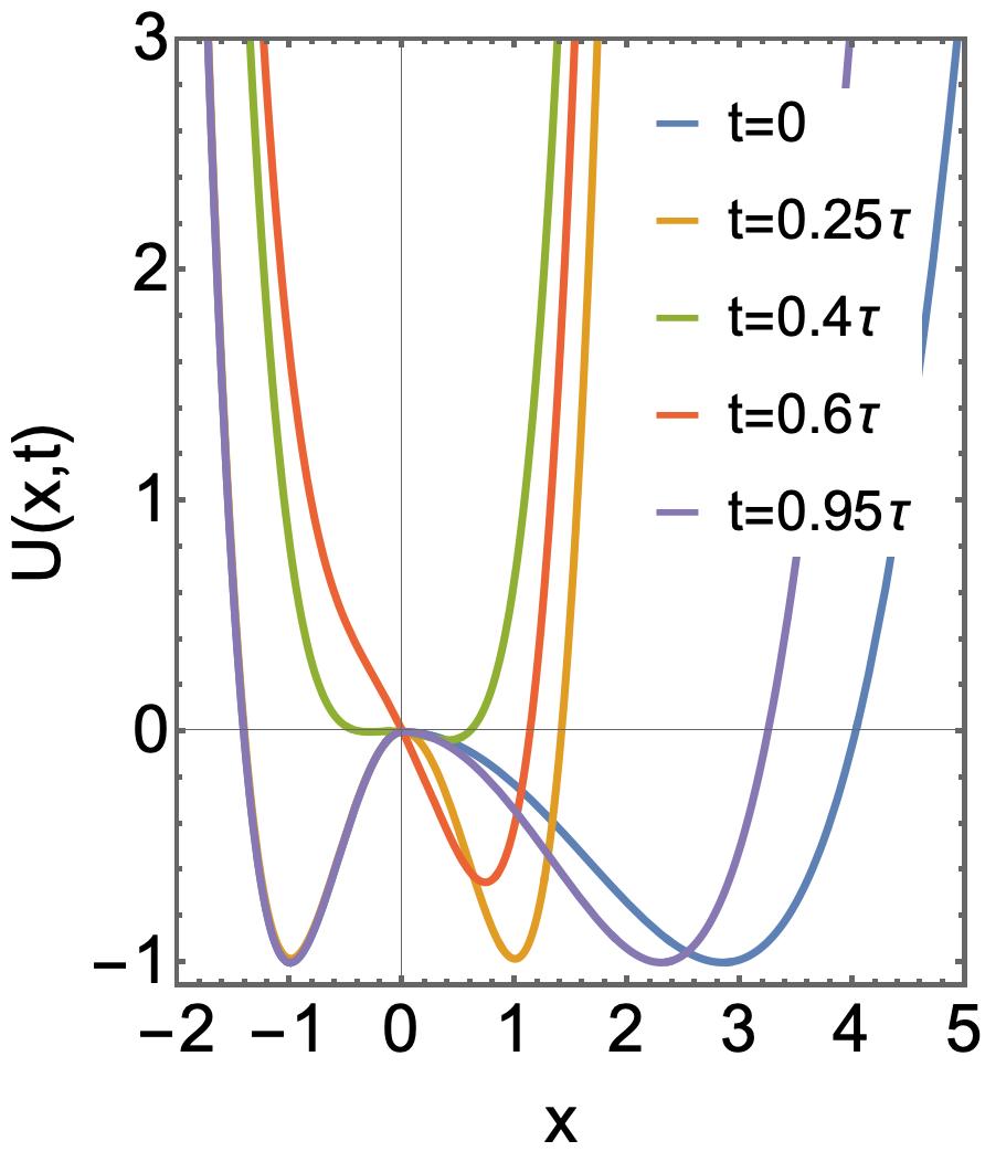
Motivated by the very good agreement between the bound and the actual entropy production in simple theoretical models, we will now turn to experimental data of a more complicated system, namely bit erasure [63]. The state of a bit can often be described by a one-dimensional Fokker-Planck equation, with a double-well potential energy landscape. This landscape can for example be produced by an optical tweezer [64], a feed-back trap [50], or a magnetic field [65, 66]. Initially, the colloidal particle can either be in the left well (state ) or in the right well (state ) of the double-well potential. By modulating this potential, one can assure that the particle always ends up the right well (state ). During this process, the expected amount of work put into the system is always bounded by the Landauer’s limit, [50]. Over the last few years, Landauer’s principle has also been tested in a more complex situation where symmetry between two states is broken [67, 68]. To add an extra layer of complexity, we consider here the scenario where this symmetry is broken by deploying an asymmetric double-well potential and we will use the data from [67] to test our bound. The system satisfies the Fokker-Planck equation
| (89) |
where is the time-dependent asymmetric double-well potential given by
| (90) | ||||
| (91) |
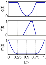
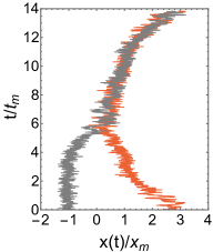
Notice that initially, the potential has its minimum located at and , where is the asymmetry factor. For , the potential is completely symmetric initially. On the other hand, for , the two wells are asymmetric and the system is out of equilibrium initially. Furthermore, the functions , and represent the experimental protocols to modulate during erasure operation. They are defined in Figure 2 and in Table 1. The experimental protocol consists of symmetrizing by changing the function , while the other two functions and are kept fixed. Then, and are changed during which the barrier is lowered, the potential is tilted and again brought back to its symmetric form at time . By this time, the particle is always at the right well. Finally, the right well is expanded to its original size with minimum located at at the end of the cycle time . The time-modulation of the potential is shown in the middle panel in Figure 2 and the experimental trajectories thus obtained are shown in the right panel.
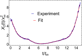
Here, we are interested in estimating the mean entropy produced during the erasure operation by using the bound in Eq. (21). For this, we take trajectories for different cycle times and measure the first two moments. The precise values of cycle time and number of trajectories considered are given in Table 2. We fit the measured moments using the basis of Chebyshev polynomials as
| (92) | |||
| (93) |
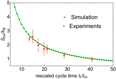
where we typically choose . For our analysis, we have rescaled the position by and with being the diffusive time scale. We have illustrated the resulting experimental plots in Figure 3. In the experiment, , , and . With the form of and in Eqs. (92) and (93), we use the formula in Eq. (21) to estimate the mean entropy produced as a function of the cycle time.
Figure 4 illustrates the primary outcome of this section. The estimated mean entropy production has been plotted for different dimensionless cycle times . The experimental results are essentially in perfect agreement with simulation results despite the very low amount of data and the non-trivial dynamics of the system. This shows that our method is well-suited to study the entropy production of general time-dependent experimental systems.
VII Conclusion
In this paper, we have constructed a general framework to derive a lower bound on the mean value of the total entropy production for arbitrary time-dependent systems described by overdamped Langevin equation. The bound, thus obtained, is given in terms of the experimentally accessible quantities, namely the (mixed) moments of the observable. If one only includes the first two moments, one gets a simple analytical expression for the lower bound, whereas including higher moments leads to a numerical scheme. We tested our results both on two analytically solvable toy models and on experimental data for bit erasure, taken from [67]. The lower bound is surprisingly close to the real entropy production, even if one only takes into account the first two moments. This makes it a perfect method to infer the entropy production and opens up the possibility to infer entropy production in more complicated processes in future research. One can for example think about biological systems, where upstream processes such as glycolytic oscillations [48] or oscillatory dynamics in transcription factors [49], can effectively lead to time-dependent thermodynamic descriptions.
We end by stressing that, although we view thermodynamic inference as the main application of our results in sections III and IV, the thermodynamic bounds Eqs. (21) and (47) are also interesting in their own rights and might lead to a broad range of applications similar to the thermodynamic speed limit and the thermodynamic uncertainty relations [6, 19].
Acknowledgement
We would like to thank Prithviraj Basak and John Bechhoefer for fruitful discussions on the paper and for providing the data used in Section VI. We also thank Jonas Berx for carefully reading the manuscript. This project has received funding from the European Union’s Horizon 2020 research and innovation program under the Marie Sklodowska-Curie grant agreement No. 847523 ‘INTERACTIONS’ and grant agreement No. 101064626 ’TSBC’ and from the Novo Nordisk Foundation (grant No. NNF18SA0035142 and NNF21OC0071284).
Appendix A Optimizing the entropy production rate
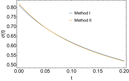
Throughout our paper, we have considered a method that gives us the optimal value of mean total entropy produced within fixed duration based on the information about moments. Here, we showcase another method that optimises the entropy production rate instead of the total dissipation . For simplicity, we focus on one dimensional case. The extension to higher dimension is quite straightforward. Moreover, we will refer to the method discussed in this section, where we minimise the rate , as Method I and the method discussed in the main text, where we minimised the total dissipation as Method II.
For systems obeying Langevin equation (1), the mean entropy production rate is given by [2]
| (94) |
In order to optimize this with given moments
| (95) | ||||
| (96) |
we consider the following objective function
| (97) | ||||
| (98) |
where for are the Lagrange multipliers corresponding to the first -moments. Now performing the minimisation , we obtain
| (99) |
such that the Lagrange multipliers can be computed by inserting this solution in Eq. (96). This gives a set of linear equations for as
| (100) |
Solving these equations completely specifies and plugging this in Eq. (94), we find the optimal entropy production rate
| (101) |
In this case also, we can get the closed form solutions for
| (102) | |||
| (103) |
where -functions are given in Eq. (20) and is the variance of . Both these results match with Eqs. (21) and (22) based on our previous method (where we optimise the total dissipation and not the rate). This means that for , the optimal value of corresponds to optimising the rate at every time instant .
In the remaining part of this section, we prove that this does not remain true for general and the two methods yield different results. To see this, let us construct corresponding to in Eq. (99) by using Eq. (6)
| (104) |
Taking a time derivative, we find
| (105) |
For general , this does not match with Eq. (29). For example, we get terms like and so on in Eq. (105) which do not appear in Eq. (29). Therefore, two methods are inequivalent for general . This in-equivalence has also been illustrated in Figure (5) for the free diffusion model considered in Eq. (64) by fixing the first four moments in Eqs. (67)-(69). In general, the method discussed in the main part of the paper will give a tighter bound for the total dissipation.
Appendix B Bound converges to exact for Gaussian distributions
In this appendix, we prove that the bound obtained in Eq. (81) converges with the exact average dissipation for Gaussian distributions. Let us begin with a general process with time-dependent potential where and are some arbitrary functions of time. This process satisfies the Langevin equation
| (106) |
If the initial position is drawn from the Gaussian distribution, then the process also admits a Gaussian distribution given by
| (107) |
Combining this with Eq. (3), we can write the probability flux as
| (108) |
Since our aim is to express completely in terms of moments and their time derivatives, we proceed to find both and in terms of moments. Using Eq. (108), it is easy to show that the variance turns out to be
| (109) |
Taking time derivative on both sides, we get
| (110) |
This expresses the first term in Eq. (108) in terms of the variance. Next we look at the second term. For this, we first express the mean as
| (111) |
and then take its time derivative to yield
| (112) |
Substituting Eqs. (110) and (112) in Eq. (108), we obtain
| (113) |
Now the expression of flux involves only first two cumulants and their time derivatives. Finally, we use Eq. (4) to get the mean total entropy produced as
| (114) |
But this is also the bound derived in Eq. (81). Hence, we conclude that converges to its exact counterpart for Gaussian distributions. We remark that although the bound is saturated for Gaussian processes, there may still be other examples of non-Gaussian processes where the bound is also saturated as long as the probability flux in given by Eq. (22).
Appendix C Derivation of Eq. (40) in dimension
This appendix presents a derivation of the Euler-Lagrange equation (40) in dimensions. For this, we first consider in Eq. (39) which is mathematically equivalent to switching from Eulerian description to the Lagrangian description in fluid mechanics [58]. Using the equivalence of two descriptions, we have
| (115) | ||||
| (116) |
Plugging , we get
| (117) |
On the other hand, putting in Eq. (115), we obtain
| (118) |
In fact, one can use to recast the optimisation of action in Eq. (38) as an optimisation problem in . To see this, we first rewrite as
| (119) |
For a small change in path , the total change in action is given by
| (120) |
where and . For optimal path, this change in action should vanish. Vanishing of the first line for arbitrary gives the Euler-Lagrange equation
| (121) |
On the other hand, we get appropriate boundary conditions by demanding vanishing of the other two lines. Since, we begin with fixed initial condition , the third line in Eq. (120) trivially goes to zero. However, the value of at the final time is not fixed which means . Hence for the change to become zero, we must have the pre-factor associated with in the second line equal to zero. Thus, we derive the following boundary conditions in time
| (122) | |||
| (123) |
Due to the linearity of Eq. (121) in , the general solution satisfies
| (124) |
In order to see that this is consistent with Eq. (121), we take its time derivative and compare the resulting with Eq. (121). This gives rise to the following relations
| (125) |
These relations ensure that Eqs. (121) and (124) are consistent with each other. To summarize, we have derived the solution for the optimal path. We now have to simply insert this solution in Eq. (118) to get the bound on total dissipation. However, before that we need to specify and functions. For this, we use the definition of moments
| (126) |
and take their time derivative to yield
| (127) | ||||
| (128) |
where . We have quoted this result in Eq. (41) of the main text.
C.1 Simplification in two dimensions
Appendix D Experimental protocols
| cycle time | m(t) | g(t) | f(t) | action |
|---|---|---|---|---|
| symmetrize potential | ||||
| lower barrier | ||||
| tilt | ||||
| raise barrier | ||||
| Untilt | ||||
| asymmetrize potential |
| Cycle time | No. of trajectories |
|---|---|
| 13.36 | 40 |
| 14.89 | 53 |
| 17.30 | 40 |
| 19.79 | 28 |
| 21.19 | 20 |
| 28.59 | 22 |
| 40.78 | 16 |
Appendix E Spatially-dependent diffusion coefficient
In this section, we will discuss how our main results change in the presence of a spatially dependent diffusion coefficient. Throughout this section, we will focus on one-dimensional systems, but the results can easily be extended to higher-dimensional systems.
In particular, we will show that one can infer the entropy production numerically, provided that one has access to the spatial dependence of the diffusion coefficient, and that one can access to . Firstly, we note that the Fokker-Planck equation (in the Stratonovich convention) is still given by Eq. (2), but that the probability flux now is given by
| (131) |
One can verify that full control over the force-field still implies full control over the probability flux.
The entropy production is now given by [69]
| (132) |
Doing the same analysis as in the main text leads to an action
| (133) |
that needs to be minimised under the constraints
| (134) |
Doing the same analysis as before leads to
| (135) | |||
| (136) | |||
| (137) |
where is given in Eq. (34) and is defined as
| (138) |
These equations can be solved numerically in exactly the same way as before, leading to a bound for systems with spatially dependent diffusion coefficients.
References
References
- [1] Seifert U 2012 Stochastic thermodynamics, fluctuation theorems and molecular machines Rep. Prog. Phys. 75 126001
- [2] Peliti L and Pigolotti S 2021 Stochastic Thermodynamics: An Introduction (Princeton University Press)
- [3] Sekimoto K 1998 Langevin equation and thermodynamics Prog. Th. Phys. Supp. 130 17–27
- [4] Seifert U 2005 Entropy Production along a Stochastic Trajectory and an Integral Fluctuation Theorem Phys. Rev. Lett. 95 040602
- [5] Hayashi K, Ueno H, Iino R and Noji H 2010 Fluctuation Theorem Applied to -ATPase Phys. Rev. Lett. 104 218103
- [6] Barato A C and Seifert U 2015 Thermodynamic uncertainty relation for biomolecular processes Phys. Rev. Lett. 114 158101
- [7] Gingrich T R, Horowitz J M, Perunov N and England J L 2016 Dissipation bounds all steady-state current fluctuations Phys. Rev. Lett. 116 120601
- [8] Proesmans K and Van den Broeck C 2017 Discrete-time thermodynamic uncertainty relation Europhys. Lett. 119 20001
- [9] Hasegawa Y and Van Vu T 2019 Fluctuation theorem uncertainty relation Phys. Rev. Lett. 123 110602
- [10] Timpanaro A M, Guarnieri G, Goold J and Landi G T 2019 Thermodynamic uncertainty relations from exchange fluctuation theorems Phys. Rev. Lett. 123 090604
- [11] Koyuk T and Seifert U 2019 Operationally accessible bounds on fluctuations and entropy production in periodically driven systems Phys. Rev. Lett. 122 230601
- [12] Proesmans K and Horowitz J M 2019 Hysteretic thermodynamic uncertainty relation for systems with broken time-reversal symmetry J. Stat. Mech.: Theory Exp. 054005
- [13] Harunari P E, Fiore C E and Proesmans K 2020 Exact statistics and thermodynamic uncertainty relations for a periodically driven electron pump J. Phys. A: Math. Theor. 53 374001
- [14] Pal S, Saryal S, Segal D, Mahesh T S and Agarwalla B K 2020 Experimental study of the thermodynamic uncertainty relation Phys. Rev. Res. 2 022044
- [15] Pietzonka P and Seifert U 2018 Universal Trade-Off between Power, Efficiency, and Constancy in Steady-State Heat Engines Phys. Rev. Lett. 120 190602
- [16] Proesmans K, Ehrich J and Bechhoefer J 2020 Finite-Time Landauer Principle Phys. Rev. Lett. 125 100602
- [17] Ilker E, Güngör O, Kuznets-Speck B, Chiel J, Deffner S and Hinczewski M 2022 Shortcuts in Stochastic Systems and Control of Biophysical Processes Phys. Rev. X 12 021048
- [18] Murugan A, Huse D A and Leibler S 2012 Speed, dissipation, and error in kinetic proofreading Proc. Natl. Acad. Sci. 109 12034-39
- [19] Shiraishi N, Funo K and Saito K 2018 Speed limit for classical stochastic processes Phys. Rev. Lett. 121 070601
- [20] Aurell E, Mejía-Monasterio C and Muratore-Ginanneschi P 2011 Optimal protocols and optimal transport in stochastic thermodynamics Phys. Rev. Lett. 106 250601
- [21] Ito S and Dechant A 2020 Stochastic time evolution, information geometry, and the cramér-rao bound Phys. Rev. X 10 021056
- [22] Aurell E, Gawedzki K, Mejía-Monasterio C, Mohayaee R and Muratore-Ginanneschi P 2012 Refined second law of thermodynamics for fast random processes J. Stat. Phys. 147 487–505
- [23] Sivak D A and Crooks G E 2012 Thermodynamic metrics and optimal paths Phys. Rev. Lett. 108 190602
- [24] Zhen Y, Egloff D, Modi K and Dahlsten O 2021 Universal bound on energy cost of bit reset in finite time Phys. Rev. Lett. 127 190602
- [25] Proesmans K, Ehrich J and Bechhoefer J 2020 Optimal finite-time bit erasure under full control Phys. Rev. E 102 032105
- [26] Van Vu T and Saito K 2022 Finite-Time Quantum Landauer Principle and Quantum Coherencee Phys. Rev. Lett. 128 010602
- [27] Dechant A 2022 Minimum entropy production, detailed balance and Wasserstein distance for continuous-time Markov processes J. Phys. A: Math.Theor. 55 094001
- [28] Falasco G and Esposito M 2020 Dissipation-time uncertainty relation Phys. Rev. Lett. 125 120604
- [29] Neri I 2022 Universal tradeoff relation between speed, uncertainty, and dissipation in nonequilibrium stationary states SciPost Physics 12 139
- [30] Kuznets-Speck B and Limmer,D T 2021 Dissipation bounds the amplification of transition rates far from equilibrium Proc. Natl. Acad. Sci. 118 e2020863118
- [31] Yan L-L et al 2022 Experimental verification of dissipation-time uncertainty relation Phys. Rev. Lett. 128 050603
- [32] Seifert U 2019 From Stochastic Thermodynamics to Thermodynamic Inference Ann. Rev. Cond. Mat. Phys. 10 171-192
- [33] Gingrich T, Rotskoff G, and Horowitz J 2017 Inferring dissipation from current fluctuations J. Phys. A 50 184004
- [34] Li J, Horowitz J M, Gingrich T R and Fakhri N 2019 Quantifying dissipation using fluctuating currents Nat. Commun. 10 1666
- [35] Manikandan S K, Gupta D and Krishnamurthy S 2020 Inferring Entropy Production from Short Experiments Phys. Rev. Lett. 124 120603
- [36] Martínez I A, Bisker G, Horowitz J M and Parrondo J M R 2019 Inferring broken detailed balance in the absence of observable currents Nat. Commun. 10 1-10
- [37] Skinner D, Dunkel J 2021 Estimating entropy production from waiting time distributions Phys. Rev. Lett. 127 198101
- [38] Harunari P E, Dutta A, Polettini M and Roldán E 2022 What to Learn from a Few Visible Transitions’ Statistics? Phys. Rev. X 12 041026
- [39] Van der Meer J, Ertel B and Seifert U 2022 Thermodynamic Inference in Partially Accessible Markov Networks: A Unifying Perspective from Transition-Based Waiting Time Distributions Phys. Rev. X 12 031025
- [40] Pietzonka P, Coghi F 2023 Thermodynamic cost for precision of general counting observables arXiv 2305.15392
- [41] Lynn C, Holmes C, Bialek W, Schwab D 2022 Decomposing the local arrow of time in interacting systems Phys. Rev. Lett. 129 118101
- [42] Lynn C, Holmes C, Bialek W, Schwab D 2022 Emergence of local irreversibility in complex interacting systems Phys. Rev. E 106 034102
- [43] Roldán E and Parrondo J M R 2010 Estimating dissipation from single stationary trajectories Phys. Rev. Lett. 105 150607
- [44] Lander B, Mehl J, Blickle V, Bechinger C and Seifert U 2012 Noninvasive measurement of dissipation in colloidal systems Phys. Rev. E. 86 030401
- [45] Otsubo S, Ito S, Dechant A and Sagawa T 2020 Estimating entropy production by machine learning of short-time fluctuating currents Phys. Rev. E. 101 062106
- [46] Van Vu T, Tuan Vo V and Hasegawa Y 2020 Entropy production estimation with optimal current Phys. Rev. E. 101 042138
- [47] Kim D-K, Bae Y, Lee S and Jeong H 2020 Learning Entropy Production via Neural Networks Phys. Rev. Lett. 125 140604
- [48] Chandra F, Buzi G and Doyle J 2011 Glycolytic oscillations and limits on robust efficiency Science 333 187
- [49] Heltberg M, Krishna S and Jensen M 2019 On chaotic dynamics in transcription factors and the associated effects in differential gene regulation Nat. Comm. 10 71
- [50] Jun Y, Gavrilov M and Bechhoefer J 2014 High-Precision Test of Landauer’s Principle in a Feedback Trap Phys. Rev. Lett. 113 190601
- [51] Freitas N, Delvenne J-C, and Esposito M 2020 Stochastic and Quantum Thermodynamics of Driven RLC Networks Phys. Rev. X 10 031005
- [52] Koyuk T and Seifert U 2020 Thermodynamic uncertainty relation for time-dependent driving Phys. Rev. Lett. 125 260604
- [53] Dechant A and Sakurai Y 2023 Thermodynamic interpretation of Wasserstein distance arXiv:1912.08405
- [54] Otsubo S, Manikandan S K, Sagawa T and Krishnamurthy S 2022 Estimating time-dependent entropy production from non-equilibrium trajectories Commun. Phys. 5 11
- [55] Lee S, Kim D-K, Park J-M, Kim W K, Park H and Lee J S 2023 Multidimensional entropic bound: Estimator of entropy production for Langevin dynamics with an arbitrary time-dependent protocol Phys. Rev. Research 5 013194
- [56] Blickle V, Speck T, Helden L, Seifert U and Bechinger, C 2006 Thermodynamics of a Colloidal Particle in a Time-Dependent Nonharmonic Potential Phys. Rev. Lett. 96 070603
- [57] Garanin D A 1997 Fokker-Planck and Landau-Lifshitz-Bloch equations for classical ferromagnets Phys. Rev. B 55 3050
- [58] Benamou J-D and Brenier Y 2000 A computational fluid mechanics solution to the Monge-Kantorovich mass transfer problem Numer. Math. 84 375-393
- [59] Villani C 2003 Topics in Optimal Transportation (American Mathematical Society, Rhode Island)
- [60] Kopp R 1962 Pontryagin maximum principle Mathematics in Science and Engineering 5 255-279
- [61] Batchelor C K and Batchelor G 2000 An introduction to fluid dynamics (Cambridge University Press)
- [62] Proesmans K 2023 Precision-dissipation trade-off for driven stochastic systems Commun. Phys. 6 226
- [63] Landauer R 1961 Irreversibility and heat generation in the computing process IBM J. Res. Develop. 5 183-191
- [64] Bérut A, Arakelyan A, Petrosyan A, Ciliberto S, Dillenschneider R and Lutz E 2012 Experimental verification of Landauer’s principle linking information and thermodynamics Nature 483 187-189
- [65] Hong J, Lambson B, Dhuey S and Bokor J 2016 Experimental test of Landauer’s principle in single-bit operations on nanomagnetic memory bits Sci. Adv. 2 e1501492
- [66] Martini L et al 2016 Experimental and theoretical analysis of Landauer erasure in nanomagnetic switches of different sizes Nano Energy 19 108-116
- [67] Gavrilov M and Bechhoefer J 2016 Erasure without Work in an Asymmetric Double-Well Potential Phys. Rev. Lett. 117 200601
- [68] Gavrilov M, Chétrite R and Bechhoefer J 2017 Direct measurement of weakly nonequilibrium system entropy is consistent with Gibbs–Shannon form Proc. Natl. Acad. Sci. 114 11097-11102
- [69] Spinney R and Ford I 2012 Entropy production in full phase space for continuous stochastic dynamics Phys. Rev. E 85 051113