Assessing the overall and partial causal well-specification of nonlinear additive noise models

Abstract

We propose a method to detect model misspecifications in nonlinear causal additive and potentially heteroscedastic noise models. We aim to identify predictor variables for which we can infer the causal effect even in cases of such misspecification. We develop a general framework based on knowledge of the multivariate observational data distribution and we then propose an algorithm for finite sample data, discuss its asymptotic properties, and illustrate its performance on simulated and real data.

1 Introduction

Nonlinear additive noise models and their heteroscedastic extensions are a popular modelling framework for causal discovery and inference. They allow to infer the true causal connections and effects from the multivariate distribution when the nonparametric model is correct; see, e.g., Hoyer et al., (2008); Peters et al., (2014) or, for heteroscedastic models, Strobl and Lasko, (2023); Immer et al., (2023). However, the conclusions can be misleading if the additive noise model is misspecified, especially in the presence of hidden confounding variables. In this paper, we define the term “causal well-specification” of additive noise models, discuss its relevance, and finally present a corresponding estimation technique for observational data.

The concept of well-specification for regression functionals in parametric regression was introduced by Buja et al., (2019). A regression functional is well-specified for a conditional target distribution if it only depends on the conditional distribution but is invariant to shifts in the predictors’ distribution. This relates to the work by Peters et al., (2016) and, hence, gives the notion of well-specification a causal interpretation. Buja et al., suggest a set of reweighting diagnostics to assess well-specification of regression functions. For the linear model, an explicit test with asymptotic level as well as precise per-covariate interpretation for certain models is presented by Schultheiss et al., (2023).

If there is no functional assumption for the additive noise model, one must rely on flexible nonparametric regression techniques that approximate the conditional mean. Considering well-specification of the conditional mean is of little use. It is by definition a property of the conditional distribution only. Hence, it is, upon existence, well-specified for arbitrary data generating mechanisms.

Thus, different concepts are needed to infer whether the estimated effects in an assumed additive noise model are causal. One of our contributions is the definition of causal well-specification and presenting its interpretation. Apart from global causal well-specification, we also define a local, i.e., per predictor version that is to be considered when the overall model does not satisfy the desired properties. This local viewpoint is of particular interest in the presence of hidden confounding, intermittent variables, or non-additive error. We propose a methodology to assess causal well-specification from observational data by relying on and exploiting conditional independence. Based on this, we derive an algorithm for finite sample data and prove its consistency. From a practical viewpoint, our estimated set of well-specified predictors (i.e., covariables) can be viewed as the one where the data is compatible (i.e., does not falsify) with the corresponding local structure of the model and its (partial) causal interpretation.

Almost no work exists on local goodness of fit or well-specification of nonlinear causal models, where local well-specification has a causal interpretation. The latter is the main goal of the present paper. The closest but weakly related work is by Maeda and Shimizu, (2021) which discusses hidden variables in causal additive noise models. They present a causal graph detection algorithm based on unconditional independence tests. This typically leads to a causal graph estimate where some of the edges remain undirected. By considering conditional independence, additional edges could be directed - at least with a conditional independence oracle which is at the basis of our approach.

2 Causal well-specification in population

We consider first the population case in which we know the joint distribution of random variables, e.g. conditional expectations and conditional independence between random variables can be perfectly assessed. This section is a stand-alone and can be used in connection with other estimation algorithms than the ones presented in Sections 3 and 6.1.

Let $\mathbf{Z}=\mathopen{}\mathclose{{}\left(Z_{1},\ldots,Z_{q}}\right)^{\top}\in\mathbb{R}^{q}$ be a random vector whose entries $Z_{j}$ follow a structural causal model (SCM) with a structure represented by a directed acyclic graph (DAG), i.e.,

$$\mathfrak{C}:\quad Z_{j}\leftarrow f_{j}\mathopen{}\mathclose{{}\left(\mathbf{Z}_{\text{PA}\mathopen{}\mathclose{{}\left(j}\right)},\mathcal{E}_{j}}\right)\ \forall j\in\mathopen{}\mathclose{{}\left\{1,\ldots,q}\right\}.$$ (1)

Here, $\text{PA}\mathopen{}\mathclose{{}\left(j}\right)$ denotes $j$’s parents according to the DAG and $\mathcal{E}_{j}$ is some noise which is jointly independent over $j$. Thus, the variables $\mathbf{Z}$ fulfil the global Markov property.

We are interested in the situation where one variable with index in $\mathopen{}\mathclose{{}\left\{1,\ldots,q}\right\}$ is the target, some of the variables are observed (potential) predictors and the rest are unobserved (potential) predictors. Let $Y$, $M$ and $N$ be the indices representing these subsets and define

$$Y\coloneqq Z_{Y},\quad\mathbf{X}\coloneqq\mathbf{Z}_{M}\in\mathbb{R}^{p},\quad\mathbf{H}\coloneqq\mathbf{Z}_{N},\quad\mathbf{X}_{\text{PA}\mathopen{}\mathclose{{}\left(Y}\right)}\coloneqq\mathbf{Z}_{M\cap\text{PA}\mathopen{}\mathclose{{}\left(Y}\right)}\quad\text{and}\quad\mathbf{H}_{\text{PA}\mathopen{}\mathclose{{}\left(Y}\right)}\coloneqq\mathbf{Z}_{N\cap\text{PA}\mathopen{}\mathclose{{}\left(Y}\right)}.$$

Note that for notational simplicity, we can absorb $\mathcal{E}_{Y}$ to be an additional variable in $\mathbf{H}_{\text{PA}\mathopen{}\mathclose{{}\left(Y}\right)}$. Therefore, $\mathbf{H}_{\text{PA}\mathopen{}\mathclose{{}\left(Y}\right)}$ always has dimensionality of at least one assuming $Y$ is not deterministic in $\mathbf{X}$. For a realisation $\mathbf{z}$ of $\mathbf{Z}$, we use the same naming convention, e.g., the realisation of $\mathbf{X}$ is then $\mathbf{x}$.

2.1 Global well-specification

The additive noise model (ANM) for $Y$ has the following structure

$$Y\leftarrow f_{\mathbf{X}Y}\mathopen{}\mathclose{{}\left(\mathbf{X}}\right)+\mathcal{E},\quad\text{where}\quad\mathbf{X}\perp\mathcal{E}.$$ (2)

We call the ANM causally well-specified if

$$\mathbf{H}_{\text{PA}\mathopen{}\mathclose{{}\left(Y}\right)}\perp\mathbf{X}\quad\text{and}\quad Y\leftarrow f_{\mathbf{X}Y}\mathopen{}\mathclose{{}\left(\mathbf{X}_{\text{PA}\mathopen{}\mathclose{{}\left(Y}\right)}}\right)+f_{\mathbf{H}Y}\mathopen{}\mathclose{{}\left(\mathbf{H}_{\text{PA}\mathopen{}\mathclose{{}\left(Y}\right)}}\right).$$ (3)

The first condition corresponds to no hidden confounding or mediation. It ensures

$$Y|\mathbf{X}=\mathbf{x}\overset{d}{=}Y|\text{do}\mathopen{}\mathclose{{}\left(\mathbf{X}\leftarrow\mathbf{x}}\right),$$

where $\overset{d}{=}$ states that two random variables have the same distribution. Assuming faithfulness, it also implies $\text{DE}\mathopen{}\mathclose{{}\left(Y}\right)\cap M=\emptyset$, where $\text{DE}\mathopen{}\mathclose{{}\left(j}\right)$ denotes $j$’s descendants according to the DAG since faithfulness ensures $\mathbf{Z}_{\text{DE}\mathopen{}\mathclose{{}\left(Y}\right)}\not\perp\mathcal{E}_{Y}\in\mathbf{H}_{\text{PA}\mathopen{}\mathclose{{}\left(Y}\right)}$. The parametrization in the second condition in (3) is not unique as constants could be moved between the two summands. We let the second have mean $0$ such that $\mathbb{E}\mathopen{}\mathclose{{}\left[Y|\mathbf{X}}\right]=f_{\mathbf{X}Y}\mathopen{}\mathclose{{}\left(\mathbf{X}_{\text{PA}\mathopen{}\mathclose{{}\left(Y}\right)}}\right)$. The condition then ensures that in the counterfactual, where we can change $\mathbf{X}$ without changing any other unobserved noise term, the outcome is exactly shifted by the difference in conditional expectation. Thus, we fully understand the effect of changing $\mathbf{X}$. Using the notation from (Peters et al.,, 2017, Chapter 6.4) and denoting point masses at $y$ by $\delta_{y}$, this can be formalized as

$$P_{Y}^{\mathfrak{C}|\mathbf{Z}=\mathbf{z};\text{do}\mathopen{}\mathclose{{}\left(\mathbf{X}\leftarrow\mathbf{x}^{\prime}}\right)}=\delta_{y^{\prime}}\quad\text{where}\quad y^{\prime}=y+\mathbb{E}\mathopen{}\mathclose{{}\left[Y|\mathbf{X}=\mathbf{x}^{\prime}}\right]-\mathbb{E}\mathopen{}\mathclose{{}\left[Y|\mathbf{X}=\mathbf{x}}\right].$$

The conditions additionally imply the following global null hypothesis that we aim to check first.

$$H_{0}:\quad\mathcal{E}\perp\mathbf{X},\quad\text{where}\quad\mathcal{E}=Y-\mathbb{E}\mathopen{}\mathclose{{}\left[Y|\mathbf{X}}\right].$$ (4)

The conditions in (3) are not necessary to fulfill (4). A prime example is with jointly Gaussian $\mathbf{Z}$: then, $H_{0}$ holds regardless of the first condition in (3) while the second condition is always fulfilled since multivariate Gaussianity implies linear additive causal effects. However, except for Gaussian $\mathbf{Z}$ or some other pathological data generating distributions, (4) is a useful proxy for (3), i.e., it allows to check whether $\mathbb{E}\mathopen{}\mathclose{{}\left[Y|\mathbf{X}}\right]$ represents a true causal effect.

To test $H_{0}$, any valid test for independence of $\mathbf{X}$ and $\mathcal{E}$ can be used.

2.2 Local well-specification

If the conditions (3) are partially violated it might still be possible to correctly understand the causal effect for some of the predictors $\mathbf{X}_{U}$ where $U\subseteq\mathopen{}\mathclose{{}\left\{1,\ldots,p}\right\}$. We say the effect of $\mathbf{X}_{U}$ is causally well-specified in the ANM if the following hold.

(A1)

The covariates in $\mathbf{X}_{U}$ are not in the Markov boundary of any variable in $\mathbf{H}_{\text{PA}\mathopen{}\mathclose{{}\left(Y}\right)}$, i.e., $\mathbf{H}_{\text{PA}\mathopen{}\mathclose{{}\left(Y}\right)}\perp\mathbf{X}_{U}|\mathbf{X}_{-U}$ (see below).

(A2)

$Y\leftarrow f_{\mathbf{X}_{U}Y}\mathopen{}\mathclose{{}\left(\mathbf{X}_{U},\mathbf{X}_{\text{PA}\mathopen{}\mathclose{{}\left(Y}\right)\setminus U}}\right)+f_{\mathbf{H}Y}\mathopen{}\mathclose{{}\left(\mathbf{H}_{\text{PA}\mathopen{}\mathclose{{}\left(Y}\right)},\mathbf{X}_{\text{PA}\mathopen{}\mathclose{{}\left(Y}\right)\setminus U}}\right)$, i.e., the causal effect is additively separable into all terms that include $\mathbf{X}_{U}$ only with observed $\mathbf{X}$ and all terms that include $\mathbf{H}$ without $\mathbf{X}_{U}$.

Here, we define the Markov boundary of a hidden variable only with respect to the measured covariates, e.g., in the structure $H_{1}\rightarrow H_{2}\rightarrow X_{1}$, $X_{1}$ would still count as part of the boundary of $H_{1}$ since it is the nearest measured descendant. Especially, if $\exists k\in M\cap\text{DE}\mathopen{}\mathclose{{}\left(Y}\right)$, all $X_{j}$ where $j\in\text{PA}\mathopen{}\mathclose{{}\left(Y}\right)$ are, up to faithfulness, in the Markov boundary of $\mathcal{E}_{Y}\in H_{\text{PA}\mathopen{}\mathclose{{}\left(Y}\right)}$ since they have a common child with respect to the measured covariates. Thus, sets containing measured parents do not fulfill (A1). Violations of faithfulness are irrelevant for (A1): if there are effects from $\mathbf{H}_{\text{PA}\mathopen{}\mathclose{{}\left(Y}\right)}$ to $\mathbf{X}_{U}$ or vice-versa that cancel out each other, we receive the same implications as if there were no such effects unless (B1) is violated; see below. Note that (A2) does not exclude the possibility that the first summand is zero, which is the case for $U\cap\text{PA}\mathopen{}\mathclose{{}\left(Y}\right)=\emptyset$.

(A1) ensures that

$$Y|\mathbf{X}_{U}=\mathbf{x}_{U},\mathbf{X}_{-U}=\mathbf{x}_{-U}\overset{d}{=}Y|\text{do}\mathopen{}\mathclose{{}\left(\mathbf{X}_{U}\leftarrow\mathbf{x}_{U}}\right),\mathbf{X}_{-U}=\mathbf{x}_{-U}$$

whenever both are defined. This follows from the second rule of do-calculus (Pearl,, 2012). After removing edges out of $\mathbf{X}_{U}$ and conditioning on $\mathbf{X}_{-U}$, dependence between $Y$ and $\mathbf{X}_{U}$ could only be induced by common unmeasured parents - a contradiction to (A1). Combined with (A2), we get two implications under an additional technical assumption

(B1)

Let $\mathopen{}\mathclose{{}\left\{A,B,C}\right\}$ be a partition of $\mathopen{}\mathclose{{}\left\{1,\ldots,q}\right\}$ in model (1). Then,

$$\mathbf{Z}_{A}\perp\mathbf{Z}_{B}|\mathbf{Z}_{C}\implies\mathbf{Z}_{A}|\mathbf{Z}_{B}=\mathbf{z}_{B},\mathbf{Z}_{C}=\mathbf{z}_{C}\ \overset{d}{=}\ \mathbf{Z}_{A}|\mathbf{Z}_{B}=\mathbf{z}^{\prime}_{B},\mathbf{Z}_{C}=\mathbf{z}_{C}\quad\forall\mathbf{z}_{B},\mathbf{z}^{\prime}_{B},\mathbf{z}_{C}.$$

This means that there are no unobservable dependencies on null sets of the observational distribution which is natural to assume except for pathological data. In general, independence only implies the latter equality for almost all $\mathbf{z}_{B},\mathbf{z}^{\prime}_{B},\mathbf{z}_{C}$.

Theorem 1.

Assume the model (1) with (B1). Let $\mathbf{X}_{U}$ be a set of covariates fulfilling (A1) and (A2), then

$$P_{Y}^{\mathfrak{C}|\mathbf{Z}=\mathbf{z};\text{do}\mathopen{}\mathclose{{}\left(\mathbf{X}_{U}\leftarrow\mathbf{x}^{\prime}_{U},\mathbf{X}_{-U}\leftarrow\mathbf{x}_{-U}}\right)}=\delta_{y^{\prime}}\quad\text{where}\quad y^{\prime}=y+\mathbb{E}\mathopen{}\mathclose{{}\left[Y|\mathbf{X}_{U}=\mathbf{x}^{\prime}_{U},\mathbf{X}_{-U}=\mathbf{x}_{-U}}\right]-\mathbb{E}\mathopen{}\mathclose{{}\left[Y|\mathbf{X}=\mathbf{x}}\right]$$

for $\mathopen{}\mathclose{{}\left(\mathbf{X}_{U}=\mathbf{x}^{\prime}_{U},\mathbf{X}_{-U}=\mathbf{x}_{-U}}\right)$ in the support of the observational distribution. Further, $H_{0,U}$ holds, where

$$H_{0,U}:\quad\mathcal{E}\perp\mathbf{X}_{U}|\mathbf{X}_{-U},\quad\text{with}\quad\mathcal{E}=Y-\mathbb{E}\mathopen{}\mathclose{{}\left[Y|\mathbf{X}}\right].$$ (5)

The first means that in the counterfactual, where we can change $\mathbf{X}_{U}$ without changing $\mathbf{X}_{-U}$, $\mathcal{E}_{Y}$, or $\mathcal{E}_{k}\ \forall k\not\in M$, the effect on $Y$ is fully determined by the shift in conditional expectation. Thus, we understand the causal effect of this theoretical intervention. Note that with (A1) and (B1), not changing $\mathbf{X}_{-U}$ and $\mathcal{E}_{k}\ \forall k\not\in M$ is equivalent to not changing $\mathbf{X}_{-U}$ and $\mathbf{H}$, i.e., all other variables apart from $\mathbf{X}_{U}$ and $Y$ remain unchanged; see also the proof in Appendix A.1. More generally, including cases where $\mathopen{}\mathclose{{}\left(\mathbf{X}_{U}=\mathbf{x}^{\prime}_{U},\mathbf{X}_{-U}=\mathbf{x}_{-U}}\right)$ is outside the support of the observational distribution, one could replace

$$\mathbb{E}\mathopen{}\mathclose{{}\left[Y|\mathbf{X}_{U}=\mathbf{x}^{\prime}_{U},\mathbf{X}_{-U}=\mathbf{x}_{-U}}\right]\quad\text{by}\quad\mathbb{E}\mathopen{}\mathclose{{}\left[Y|\text{do}\mathopen{}\mathclose{{}\left(\mathbf{X}_{U}\leftarrow\mathbf{x}^{\prime}_{U}}\right),\mathbf{X}_{-U}=\mathbf{x}_{-U}}\right]$$

which are equivalent if both are defined as discussed above. However, this is not estimable outside the data support.

We note that the implication of (A1) would be of practical interest on its own. However, as we do not know of any useful proxy for it that can be calculated by the observational distribution, we always consider the combination of (A1) and (A2) as the object of interest.

The local null hypothesis $H_{0,U}$ that can be checked by the observational distribution alone serves as a proxy for (A1) and (A2). Again, a multivariate Gaussian distribution is an example where (5) holds true regardless of (A1). However, for other data generating distributions, we consider (5) to be a good proxy to see whether (A1) and (A2) might hold.

In general, (5) does not imply that the ANM (2) with only $\mathbf{X}_{U}$ as predictors is causally well-specified. Therefore, this set cannot be found by looping over all subsets of $\mathbf{X}$ and testing (4).

Consider Figure 1. In the left structure, $W=\mathopen{}\mathclose{{}\left\{2}\right\}$ if (A2) holds for $X_{2}$. But, $X_{2}\rightarrow Y$ is not a causally well-specified ANM unless faithfulness is violated, i.e. $X_{2}\perp H$. Similarly, on the right, it holds $W=\mathopen{}\mathclose{{}\left\{1}\right\}$ if (A2) holds for $X_{1}$. Note also that there is an unobserved causal path (Maeda and Shimizu,, 2021) from $X_{1}$ to $Y$. Nevertheless, the edge is detectable when considering conditional independence criteria.

Figure 1: Left: Structure with a hidden confounder. Right: Structure with a hidden mediator.

Of most interest is the set

$$W\coloneqq\underset{U:H_{0,U}\ \text{is true}}{\text{arg max}}\mathopen{}\mathclose{{}\left|U}\right|.$$ (6)

As $\mathopen{}\mathclose{{}\left\{1,\ldots p}\right\}\setminus W$ defines a Markov boundary of $\mathcal{E}$, uniqueness of $W$ is equivalent to uniqueness of the Markov boundary. This is implied if the so-called intersection property holds (Pearl,, 1988, Chapter 3).

(B2)

$$\mathcal{E}\perp\mathbf{X}_{A}|\mathbf{X}_{B},\mathbf{X}_{C}\quad\text{and}\quad\mathcal{E}\perp\mathbf{X}_{B}|\mathbf{X}_{A},\mathbf{X}_{C}\implies\mathcal{E}\perp\mathbf{X}_{A},\mathbf{X}_{B}|\mathbf{X}_{C}$$

for any partition $A,B,C$ of $\mathopen{}\mathclose{{}\left\{1,\ldots,p}\right\}$.

This is guaranteed if $\mathbf{X}$ has full support with respect to the product of the domains of the individual $X_{j}$. Necessary, strictly weaker conditions are discussed by Peters, (2015). One estimation strategy would be to consider the individual hypothesis

$$\begin{split}H_{0,j}:\quad\mathcal{E}&\perp X_{j}|\mathbf{X}_{-j},\quad\text{where}\quad\mathcal{E}=Y-\mathbb{E}\mathopen{}\mathclose{{}\left[Y|\mathbf{X}}\right]\\ \tilde{W}&=\mathopen{}\mathclose{{}\left\{j:H_{0,j}\ \text{is true}}\right\}.\end{split}$$ (7)

We can relate this to the Markov boundary.

Theorem 2.

Let $W$ be as in (6) and $\tilde{W}$ as in (7). Then, $W\subseteq\tilde{W}$. If the intersection property (B2) holds, $W=\tilde{W}$.

We emphasize that the characterizations in this Section 2 provide the fundamental basis to define the concepts of global and local causal well-specification. This then enables the construction of algorithms that aim to estimate causal well-specification based on finite sample observational data, as discussed next.

3 Estimating the set of well-specified predictor variables

We subsequently focus on a specific method to assess conditional dependence. Of course, different estimators could be used as well. The intuition of how conditional independence relates to causal well-specification stays the same.

Throughout this section, we assume that we have n i.i.d. observations $\mathbf{x}=\begin{pmatrix}\mathbf{x}_{1},\ldots,\mathbf{x}_{n}\end{pmatrix}^{\top}\in\mathbb{R}^{n\times p}$ and $\mathbf{y}=\begin{pmatrix}y_{1},\ldots,y_{n}\end{pmatrix}^{\top}\in\mathbb{R}^{n}$ of $\mathbf{X}$ and $Y$ respectively. Also, define the unobserved $\epsilon_{i}=y_{i}-\mathbb{E}\mathopen{}\mathclose{{}\left[Y|\mathbf{X}=\mathbf{x}_{i}}\right]$.

3.1 Making use of FOCI (Feature Ordering by Conditional Independence

One estimation strategy would be to test the hypotheses in (7) for all $j$. Conditional independence testing is a hard problem on its own; here, it is even more challenging as we need to rely on estimated residuals rather than the error terms directly. Instead, we use FOCI (Feature Ordering by Conditional Independence) by Azadkia and Chatterjee, (2021). This method estimates a Markov blanket of a target variable with high probability for large enough sample size. Thus, it can find a superset of the Markov boundary of $\mathcal{E}$, say, $\hat{S}$, such that $\mathopen{}\mathclose{{}\left(\mathopen{}\mathclose{{}\left\{1,\ldots,p}\right\}\setminus\hat{S}}\right)\subseteq W$. Still, we need to deal with the harder version of applying FOCI to the estimated residuals $\hat{\boldsymbol{\epsilon}}$ instead of the true, unobserved errors $\boldsymbol{\epsilon}$.

The global null hypothesis in (4) is easier to infer with unconditional independence tests than the conditional analog in (5), even when using estimated residuals as discussed in Pfister et al., (2018). We use this global test as well in our proposed algorithms below.

In general, we require some sort of consistency for our regression estimates and our discussion allows any reasonable choice of regression (machine learning) techniques. While as in the population case rejections of the null hypothesis could only be due to hidden confounding or additively non-separable functions, one must always consider insufficient explicative power of the applied regression (machine learning) method as a further reason in the finite sample case.

We consider two different algorithms.

Algorithm 1 In-sample FOCI

Input i.i.d. data $\mathbf{x}\in\mathbb{R}^{n\times p}$ and $\mathbf{y}\in\mathbb{R}^{n}$, and function $g\mathopen{}\mathclose{{}\left(\cdot}\right)$
      Output estimated set of variables for which null hypothesis (5) is rejected $\hat{S}$

1:Get an estimate $\hat{f}\mathopen{}\mathclose{{}\left(\mathbf{X}}\right)$ for $\mathbb{E}\mathopen{}\mathclose{{}\left[Y|\mathbf{X}}\right]$ using a certain regressor

2:Estimate the residuals as $\hat{\boldsymbol{\epsilon}}=\mathbf{y}-\hat{f}\mathopen{}\mathclose{{}\left(\mathbf{x}}\right)$

3:Apply FOCI (Azadkia and Chatterjee,, 2021) to the data $\mathopen{}\mathclose{{}\left(g\mathopen{}\mathclose{{}\left(\hat{\boldsymbol{\epsilon}}}\right),\mathbf{x}}\right)$ to get the set $\hat{S}$

Algorithm 2 Sample splitting FOCI

Input i.i.d. data $\mathbf{x}\in\mathbb{R}^{n\times p}$ and $\mathbf{y}\in\mathbb{R}^{n}$, and function $g\mathopen{}\mathclose{{}\left(\cdot}\right)$
      Output estimated set of variables for which null hypothesis (5) is rejected $\hat{S}$

1:Split the data uniformly at random into two disjoint parts of sizes $\lfloor n/2\rfloor$ and $\lceil n/2\rceil$, say, $\mathopen{}\mathclose{{}\left(\mathbf{x}^{\mathopen{}\mathclose{{}\left(1}\right)},\mathbf{y}^{\mathopen{}\mathclose{{}\left(1}\right)}}\right)$ and $\mathopen{}\mathclose{{}\left(\mathbf{x}^{\mathopen{}\mathclose{{}\left(2}\right)},\mathbf{y}^{\mathopen{}\mathclose{{}\left(2}\right)}}\right)$

2:Get an estimate $\hat{f}\mathopen{}\mathclose{{}\left(\mathbf{X}}\right)$ for $\mathbb{E}\mathopen{}\mathclose{{}\left[Y|\mathbf{X}}\right]$ using a certain regressor on the data $\mathopen{}\mathclose{{}\left(\mathbf{x}^{\mathopen{}\mathclose{{}\left(1}\right)},\mathbf{y}^{\mathopen{}\mathclose{{}\left(1}\right)}}\right)$

3:Estimate the residuals as $\hat{\boldsymbol{\epsilon}}^{\mathopen{}\mathclose{{}\left(2}\right)}=\mathbf{y}^{\mathopen{}\mathclose{{}\left(2}\right)}-\hat{f}\mathopen{}\mathclose{{}\left(\mathbf{x}^{\mathopen{}\mathclose{{}\left(2}\right)}}\right)$

4:Apply FOCI (Azadkia and Chatterjee,, 2021) to the data $\mathopen{}\mathclose{{}\left(g\mathopen{}\mathclose{{}\left(\hat{\boldsymbol{\epsilon}}^{\mathopen{}\mathclose{{}\left(2}\right)}}\right),\mathbf{x}^{\mathopen{}\mathclose{{}\left(2}\right)}}\right)$ to get the set $\hat{S}$

For notational simplicity, we call the data that is input to FOCI $\mathopen{}\mathclose{{}\left(\hat{\boldsymbol{\epsilon}},\mathbf{x}}\right)$ in our theoretical derivations regardless of the applied algorithm, i.e., we omit the superscript in the splitting case. The advantage of Algorithm 2 is that the residuals estimated on the hold-out split are still i.i.d. which simplifies things, at least analytically. Furthermore, the sample splitting idea enables further favourable algorithms to be presented in Section 3.3.

For power purposes, it can be advantageous to consider a certain non-monotonic transformation $g\mathopen{}\mathclose{{}\left(\mathcal{E}}\right)$ as input to FOCI. In particular, we suggest the absolute value function. For this, we provide a precise result for symmetric data below. Although exact symmetry is hardly the case except for toy examples, the intuition is that the dependence of $\mathcal{E}$ on $\mathbf{X}$ can be mainly in the second moment, i.e., the scale. Hence, the absolute value transform is then beneficial. For our general results, we assume that $g\mathopen{}\mathclose{{}\left(\cdot}\right)$ is an $l$-Lipschitz function whose level sets have Lebesgue measure $0$.

Use the definitions (2.1) and (11.1) in (Azadkia and Chatterjee,, 2021) for $T\mathopen{}\mathclose{{}\left(\cdot}\right)$ and $Q\mathopen{}\mathclose{{}\left(\cdot}\right)$. FOCI greedily increases the set of predictors to maximize $Q$.

Proposition 1.

Let $U\subseteq\mathopen{}\mathclose{{}\left\{1,\ldots,p}\right\}$. If $\mathcal{E}|\mathbf{X}_{U}$ has a continuous and symmetric (around 0) distribution, it holds

$$T\mathopen{}\mathclose{{}\left(\mathopen{}\mathclose{{}\left|\mathcal{E}}\right|,\mathbf{X}_{U}}\right)=4T\mathopen{}\mathclose{{}\left(\mathcal{E},\mathbf{X}_{U}}\right)\quad\text{and}\quad Q\mathopen{}\mathclose{{}\left(\mathopen{}\mathclose{{}\left|\mathcal{E}}\right|,\mathbf{X}_{U}}\right)=4Q\mathopen{}\mathclose{{}\left(\mathcal{E},\mathbf{X}_{U}}\right).$$

These larger population values can improve the algorithm’s performance.

3.2 Asymptotic results

We generally make the following assumptions for applying FOCI to an estimated $\hat{\boldsymbol{\epsilon}}$.

(B3)

$\mathopen{}\mathclose{{}\left|\hat{\epsilon}_{i}-\epsilon_{i}}\right|={\scriptstyle\mathcal{O}_{p}}\mathopen{}\mathclose{{}\left(1}\right)$

(B4)

$\mathcal{E}$ is a continuous random variable.

(B5)

$\nexists U\subseteq\mathopen{}\mathclose{{}\left\{1,\ldots,p}\right\}$ such that $\mathbf{X}_{U}\not\perp\mathcal{E}|\mathbf{X}_{-U}$ but $\mathbf{X}_{U}\perp g\mathopen{}\mathclose{{}\left(\mathcal{E}}\right)|\mathbf{X}_{-U}$.

The probability in (B3) is with respect to both the regression estimate and the new data point $i$. The assumption is slightly different depending on which algorithm is applied. Apart from invoking (B4) for the proofs, we provide a simple example in Section 3.2.1 to show that discrete distributions can lead to inconsistency.

The main proof ingredient for adapting the results to our setting is showing that for random indices $i$ and $l$ the probability that the estimated residuals imply a different relative ordering than the true residuals approaches $0$.

With sample splitting, we obtain a consistency result analogous to Azadkia and Chatterjee, (2021).

Theorem 3.

Suppose that the regularity assumptions (A1’) and (A2’) (Azadkia and Chatterjee,, 2021) for the data $\mathopen{}\mathclose{{}\left(g\mathopen{}\mathclose{{}\left(\mathcal{E}}\right),\mathbf{X}}\right)$ hold as well as conditions (B2) - (B5). Let $\hat{S}$ be the output of Algorithm 2. There are positive real numbers $L_{1}$, $L_{2}$ and $L_{3}$ that do not depend on the sample size such that

$$\mathbb{P}\mathopen{}\mathclose{{}\left(\hat{S}\supseteq\mathopen{}\mathclose{{}\left\{1,\ldots,p}\right\}\setminus W}\right)\geq 1-L_{1}p^{L_{2}}\exp\mathopen{}\mathclose{{}\left(-L_{3}n}\right).$$

Without sample splitting, $\mathopen{}\mathclose{{}\left(g\mathopen{}\mathclose{{}\left(\hat{\boldsymbol{\epsilon}}}\right),\mathbf{x}_{U}}\right)$ are not independent copies. Therefore, the bounded difference inequality (McDiarmid et al.,, 1989) which is applied to obtain the exponential probability decay cannot be used. Nevertheless, convergence in probability is still true.

Theorem 4.

Assume the conditions of Theorem 3. Let $\hat{S}$ be the output of Algorithm 1. Then,

$$\underset{n\rightarrow\infty}{\lim}\mathbb{P}\mathopen{}\mathclose{{}\left(\hat{S}\supseteq\mathopen{}\mathclose{{}\left\{1,\ldots,p}\right\}\setminus W}\right)=1.$$

This result is derived by a simple application of the Markov inequality instead of the bounded difference inequality. As the $\mathopen{}\mathclose{{}\left(g\mathopen{}\mathclose{{}\left(\hat{\boldsymbol{\epsilon}}}\right),\mathbf{x}_{U}}\right)$ become decreasingly dependent from another with increasing sample size, we conjecture that the true convergence rate could be similar to the one for sample splitting.

3.2.1 Discrete $\mathcal{E}$

For our results, we invoked assumption (B4), i.e., the error term is a continuous random variable. A simple toy example shows that a discrete random variable might invalidate the asymptotic guarantees. Use the definition (2.1) in Azadkia and Chatterjee, (2021) for $T\mathopen{}\mathclose{{}\left(\cdot}\right)$, i.e., $T\mathopen{}\mathclose{{}\left(\mathcal{E},X}\right)=0$ if and only if $\mathcal{E}$ and $X$ are independent. Let $T_{n}\mathopen{}\mathclose{{}\left(\cdot}\right)$ be its suggested sample estimate.

Proposition 2.

Let $X$ be a bounded, continuous random variable and $\mathcal{E}$ a centered random variable that is uniformly distributed over a discrete set of size $k>1$ independent from $X$ such that $T\mathopen{}\mathclose{{}\left(\mathcal{E},X}\right)=0$. Let $Y\leftarrow X\beta+\mathcal{E}$ for some $\beta\neq 0$. Apply linear least squares regression, which fulfils (B3), to $n$ i.i.d. copies $\mathopen{}\mathclose{{}\left(\mathbf{y},\mathbf{x}}\right)$ to get the estimates $\hat{\boldsymbol{\epsilon}}$. It holds

$$\mathbb{E}\mathopen{}\mathclose{{}\left[T_{n}\mathopen{}\mathclose{{}\left(\hat{\boldsymbol{\epsilon}},\mathbf{x}}\right)}\right]\overset{n\rightarrow\infty}{\rightarrow}\dfrac{1}{k^{2}}>0.$$

3.3 Practical algorithm

Although we can consistently find a Markov blanket (but not necessarily the minimal one) using Algorithms 1 or 2 as the sample size grows, there are several drawbacks to that. First, there is no protection against including superfluous variables into $\hat{S}$ and typically this happens with non-negligible probability. Second, for low sample sizes, $\hat{S}$ can miss out on some variables.

To partially remedy these issues, we incorporate ideas from multisplitting (Meinshausen et al.,, 2009) and stability selection (Meinshausen and Bühlmann,, 2010). We apply Algorithm 2 repeatedly with several random data partitions. Inspired by Shah and Samworth, (2013) who suggest using “complementary pairs”, i.e., both halves of every split, we let each halve be used once for estimating the conditional mean and once for independence testing.

Algorithm 3 Variable selection with multiple splits

Input i.i.d. data $\mathbf{x}\in\mathbb{R}^{n\times p}$ and $\mathbf{y}\in\mathbb{R}^{n}$, function $g\mathopen{}\mathclose{{}\left(\cdot}\right)$, number of repetitions $B$, and significance levels $\alpha$ and $\tilde{\alpha}$.
      Output estimated set of variables with causally well-specified effect $\hat{W}$

1:$n_{j}=0\ \forall j=1,\ldots,p$

2:for $b=1$ to $B$ do

3:     Split the data uniformly at random into two disjoint parts of sizes $\lfloor n/2\rfloor$ and $\lceil n/2\rceil$, say, $\mathopen{}\mathclose{{}\left(\mathbf{x}^{\mathopen{}\mathclose{{}\left(1}\right)},\mathbf{y}^{\mathopen{}\mathclose{{}\left(1}\right)}}\right)$ and $\mathopen{}\mathclose{{}\left(\mathbf{x}^{\mathopen{}\mathclose{{}\left(2}\right)},\mathbf{y}^{\mathopen{}\mathclose{{}\left(2}\right)}}\right)$

4:     Get an estimate $\hat{f}\mathopen{}\mathclose{{}\left(\mathbf{X}}\right)$ for $\mathbb{E}\mathopen{}\mathclose{{}\left[Y|\mathbf{X}}\right]$ using a certain regressor on the data $\mathopen{}\mathclose{{}\left(\mathbf{x}^{\mathopen{}\mathclose{{}\left(1}\right)},\mathbf{y}^{\mathopen{}\mathclose{{}\left(1}\right)}}\right)$

5:     Estimate the residuals as $\hat{\boldsymbol{\epsilon}}^{\mathopen{}\mathclose{{}\left(2}\right)}=\mathbf{y}^{\mathopen{}\mathclose{{}\left(2}\right)}-\hat{f}\mathopen{}\mathclose{{}\left(\mathbf{x}^{\mathopen{}\mathclose{{}\left(2}\right)}}\right)$

6:     Apply the HSIC test to the data $\mathopen{}\mathclose{{}\left(\hat{\boldsymbol{\epsilon}}^{\mathopen{}\mathclose{{}\left(2}\right)},\mathbf{x}^{\mathopen{}\mathclose{{}\left(2}\right)}}\right)$ to get the p-value $p^{b}$.

7:     Apply FOCI (Azadkia and Chatterjee,, 2021) to the data $\mathopen{}\mathclose{{}\left(g\mathopen{}\mathclose{{}\left(\hat{\boldsymbol{\epsilon}}^{\mathopen{}\mathclose{{}\left(2}\right)}}\right),\mathbf{x}^{\mathopen{}\mathclose{{}\left(2}\right)}}\right)$ to get the set $\hat{S}^{b}$

8:     Swap the roles of $\mathopen{}\mathclose{{}\left(\mathbf{x}^{\mathopen{}\mathclose{{}\left(1}\right)},\mathbf{y}^{\mathopen{}\mathclose{{}\left(1}\right)}}\right)$ and $\mathopen{}\mathclose{{}\left(\mathbf{x}^{\mathopen{}\mathclose{{}\left(2}\right)},\mathbf{y}^{\mathopen{}\mathclose{{}\left(2}\right)}}\right)$ and repeat the previous steps to get $p^{B+b}$ and $\hat{S}^{B+b}$

9:Combine the p-values $p^{1},\ldots p^{2B}$ (Meinshausen et al.,, 2009) and get the model p-value $p^{0}$.

10:if $p^{0}>\alpha$ then

11:     $\hat{W}=\mathopen{}\mathclose{{}\left\{1,\ldots,p}\right\}$

12:else

13:     $\hat{W}=\emptyset$

14:     for $j=1$ to $p$ do

15:         $n_{j}=\sum_{b=1}^{2B}j\in\hat{S}^{b}$      

16:     $\bar{n}=\sum_{j=1}^{p}n_{j}/p$

17:     $n^{\min}=\underset{j:n_{j}\geq\bar{n}}{\min n_{j}}$

18:     for $j=1$ to $p$ do

19:         if $n_{j}<\bar{n}$ and $proportion.test\mathopen{}\mathclose{{}\left(n_{j},n^{min},2B}\right)\leq\tilde{\alpha}$ then

20:              $\hat{W}=\hat{W}\cup j$               

As unconditional independence is easier to assess than conditional independence, we first test for $H_{0}$ as in (4). For this, we apply the test by Pfister et al., (2018) and we combine the p-values over the different splits as suggested by Meinshausen et al., (2009). Only if the global model is rejected, the individual covariates are inspected.

If we cannot trust the overall model, we only consider the effects of variables that are selected substantially less than others by the FOCI algorithm to be causally well-specified. We split the variables into two groups: those that are selected by FOCI below average over the splits and the others. For the latter group, we reject $H_{0,j}$. Each variable from the first group we compare to the least selected variable from the second group with some proportion test such as Fisher’s exact test. The variables that show significant differences are added to the estimated well-specified set $\hat{W}$. Notably, there is no exact interpretation of the significance level used for these tests, but the intuition that a lower significance level leads to fewer false positives in the set $\hat{W}$ remains true. In contrast, a lower significance level for the preceding test of the global model leads to the methods becoming more liberal.

The intuition behind splitting at the mean is the following. For large enough sample size, the necessary variables are selected by FOCI in almost every split, see Theorem 3, while the variables with causally well-specified effect could be selected with some probability much lower than $1$. The mean separates the two groups and there is a significant difference in the selection fraction of the two groups. For a low sample size, the behaviour of FOCI is more random. However, as long as no variables stand out, we do not add any to $\hat{W}$, i.e., if $H_{0,j}$ is not true, the probability $\mathbb{P}\mathopen{}\mathclose{{}\left(j\in\hat{W}}\right)$ is moderately low. However, it is lower bounded by the type II error of the global test. This is fundamental to our idea. If the sample size is such that the global test, i.e., unconditional independence testing, does not work well yet, the local analysis is also not of much use.

We summarize the procedure in Algorithm 3.

4 Simulation example

We evaluate the method on a simple SCM represented by the DAG in Figure 2. We let the causal effects be non-monotonic functions of the form

$$f\mathopen{}\mathclose{{}\left(X_{j}}\right)=\alpha_{1}\mathopen{}\mathclose{{}\left|X_{j}}\right|^{\beta_{1}}\text{sign}\mathopen{}\mathclose{{}\left(X_{j}}\right)+\alpha_{2}\mathopen{}\mathclose{{}\left|X_{j}}\right|^{\beta_{2}},$$

where the parameters are randomly sampled and differ for every simulation run. The causal effect on $Y$ is additive in the parents. We standardize and normalize the effects. The additive error terms are either normal, uniform, or Laplace with variance $1$ for the root nodes and $1/4$ for the others. The different distributions are randomly assigned to the different nodes; two of each.

We consider all possible subsets of size $3$ as observed predictors. Denote this observed subset by $M$. For $M=\mathopen{}\mathclose{{}\left\{1,2,3}\right\}$ and $M=\mathopen{}\mathclose{{}\left\{1,3,5}\right\}$ the additive noise model is causally well-specified.

Figure 2: DAG representing the SCM in the simulation

We consider $100$ different random setups for sample sizes $10^{2}$ to $10^{5}$. For each, we consider all possible $M$. To get $\hat{W}$ we apply Algorithm 3 with $B=25$ splits and the absolute value function as $g\mathopen{}\mathclose{{}\left(\cdot}\right)$.

For the regression, we apply eXtreme Gradient Boosting implemented in the R-package xgboost (Chen et al.,, 2021). We use the respective left-out split of the data for early stopping when fitting the regression functions. This is a slight violation of our theoretical algorithm where the residuals are perfectly independent. We use the authors’ implementation of FOCI (Azadkia et al.,, 2021) and dHSIC (Pfister and Peters,, 2019).

For the predictor sets where global causal well-specification does not hold true, we consider the false positive rate (FPR) $\hat{\mathbb{P}}\mathopen{}\mathclose{{}\left(j\in\hat{W}|j\not\in W}\right)$ and the true positive rate (TPR) $\hat{\mathbb{P}}\mathopen{}\mathclose{{}\left(j\in\hat{W}|j\in W}\right)$ for adding predictors to the set $\hat{W}$. Here, $\hat{\mathbb{P}}\mathopen{}\mathclose{{}\left(\cdot}\right)$ denotes the empirical probability over our simulation runs. We fix $\alpha=0.05$ and consider varying values of $\tilde{\alpha}$. The resulting rates are on the left in Figure 3.

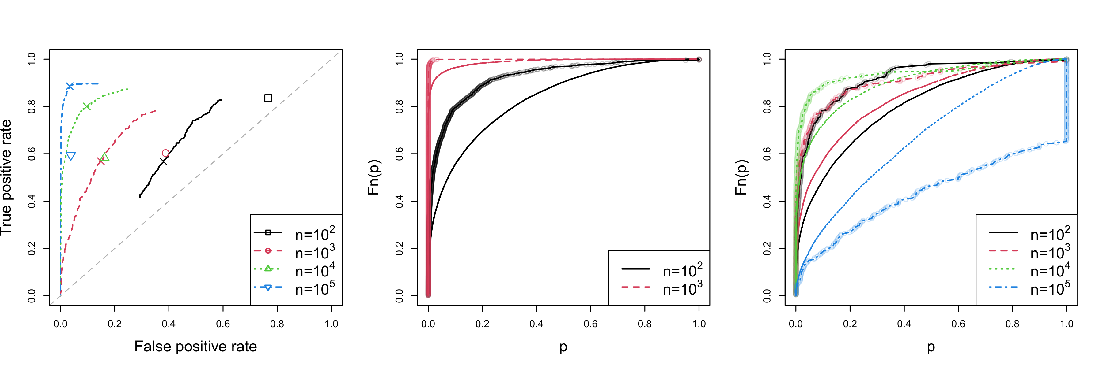
Figure 3: The results are based on $100$ simulation runs. On the left: False positive rate versus true positive rate obtained with Algorithm 3 for varying $\tilde{\alpha}$ and $\alpha=0.05$. The crosses correspond to $\tilde{\alpha}=0.01$. The other symbols describe the performance of Algorithm 2. In the middle: empirical cumulative distribution function of the p-values obtained with HSIC. We compare the raw p-values from each split (lines only) to the cumulated p-value per simulation run (lines with dots). On the right: the same for the models fulfilling $H_{0}$.

For $n=10^{2}$, a low FPR is not attainable because the p-values for (4) are not reliably small enough, and Algorithm 3 often terminates before considering the individual covariates. However, even for this low sample size, we get a performance that is clearly better than random guessing. For large sample sizes, the FPR becomes very low which is in agreement with Theorem 3. The lack of power is mainly due to the subsets of predictors with $\mathopen{}\mathclose{{}\left|W}\right|>1$. FOCI chooses superfluous covariates with non-vanishing probability for every sample size. Hence, the two covariates with causally well-specified effects may be selected with a frequency that differs a lot between the two. If one then appears to be more similar to the covariate with not well-specified effect, our algorithm misses out on this such that $\hat{W}\subset W$.

For comparison, we also show the results if we instead only consider a single random split where $50\%$ of the data is used to estimate the residuals and the other $50\%$ to assess independence. If $H_{0}$ is rejected we apply Algorithm 2 (using the same splits) and choose $\hat{W}$ to be the complement of the set chosen by FOCI. Except for $n=10^{2}$, this lies below the curve for multiple splits, i.e., there is an $\tilde{\alpha}$ that is better in terms of both FPR and TPR. Further, our default choice $\tilde{\alpha}=0.01$ is more conservative. For large enough sample size, using $\tilde{\alpha}=0.01$ leads to more power than considering a single split. Hence, even though the problem is hard in general, aggregating information over multiple random splits of the same dataset can lead to a performance boost.

We also evaluate the testing of $H_{0}$ (4). For this, we show the empirical cumulative distribution function of the obtained p-values in the middle of Figure 3. We consider the p-value aggregated over the splits as well as the individual p-values considering single splits. For the largest sample sizes, the distribution of both is visibly not distinguishable from a point mass at $0$. We omit this in the plot for the sake of overview. For $n=10^{2}$ and $n=10^{3}$, aggregating the p-values over splits helps to reject the global model for most possible significance levels. The acceptance rate for the global model poses a lower bound to the attainable FPR for every subsequent per-covariate analysis. For $n=10^{2}$ and $\alpha=0.05$, this rate is around $0.56$ for single splits and reduced to roughly $0.33$ by aggregating. This confirms the usefulness of the multisplitting idea.

We also consider the distribution of the p-values for the two subsets of predictors that yield causally well-specified models. This is shown on the right side of Figure 3. We see that the raw p-values are too liberal. By construction, this effect is enhanced by aggregation over the splits. For increasing sample size, there are two competing effects. The regression approximation becomes better leading to less dependent residuals. But, the tests become more powerful in detecting spurious dependence. As the HSIC implementation cannot handle $5\cdot 10^{4}$ samples, we only test with $10^{4}$ samples per split. Hence, the p-values for $n=10^{5}$ are likely more liberal theoretically. In summary, we see that testing for (4) is already difficult per se. However, one can also see it the other way around: if the regression is unable to render the residuals independent one should not trust the obtained function even if there was a true underlying ANM.

In this example, fitting only additive functions with no interactions between the measured covariates leads to the same conclusion given perfect regression fit and independence tests. Hence, if one restricts the analysis to additive functions due to pre-knowledge or just by assumption the problem could become easier. When applying GAM regression as implemented in mgcv (Wood,, 2011), the results for the causally not well-specified predictor sets remain qualitatively similar. The p-values for the models fulfilling $H_{0}$ are still visibly clearly not uniformly distributed. But, they become less liberal. This is as finding the true conditional mean and hence the true independent residuals becomes easier. For $n=10^{5}$ the distribution of the raw p-values is sufficiently close to uniform such that the aggregated p-values are even super-uniform. Again, this needs to be taken with a grain of salt as not all samples can be used for testing independence.

5 Real data analysis

We consider the K562 dataset provided by Replogle et al., (2022). We follow the preprocessing in the benchmark of Chevalley et al., (2022). Then, the dataset contains 162,751 measurements of the activity of 622 genes: 10,691 of the measurements are taken in a purely observational environment while the remaining are obtained under various interventions. For each gene, there exists an environment where it has been intervened on by a knock down using CRISPRi (Larson et al.,, 2013), i.e., its activity is reduced. As our method is designed for i.i.d. data, we only consider the observational environment henceforth. With the interventions, some sanity checks of our findings are possible as discussed below.

We make a pre-selection of the measured covariates before applying our method. There are $28$ genes that are active, i.e., greater than $0$, in each measurement in the observational sample. We restrict our analysis to these and call them $X_{1}$ to $X_{28}$ for simplicity. Within these $28$, we estimate Markov blankets using FOCI. For each of the $28$ genes, two estimates are implied: all the genes selected by FOCI when this covariate is the target as well as all the genes for which this covariate is in the output of FOCI. As target, say $Y$, we choose the one with the highest agreement between the two estimated sets in terms of intersection size relative to the size of the union. For the target $Y$, we then consider the intersection of the Markov blankets mentioned above (where $Y$ is the target or appears in the output of FOCI). This results in three predictors, $X_{10}$, $X_{12}$, $X_{15}$.

With the selected target and predictors we run Algorithm 3 with $B=25$ splits using xgboost for regression. There is a strong indication against the global null hypothesis (4) with a p-value of roughly $10^{-27}$. Hence, we proceed to the per-covariate analysis. Covariate $X_{15}$ is in $\hat{S}^{b}$ 41 out of 50 times while as for the others it is only 22 ($X_{10}$) and 19 ($X_{12}$). Hence, the effects of the latter appear to be causally well-specified and we get the set $\hat{W}=\mathopen{}\mathclose{{}\left\{X_{10},X_{15}}\right\}$ when running Algorithm 3 with our suggested default of $\tilde{\alpha}=0.01$.

To assess the success of our method, we now consider the available interventional data. Comparing the distribution of $X_{k}$ when the activity of $X_{j}$ is reduced by an external intervention to its observational distribution, gives an assessment of whether there is a causal effect from $X_{j}$ to $X_{k}$. We do this using a Mann-Whitney U test. Intervening on any of the three predictor covariates appears to highly influence the activity of $Y$ with p-values of the order $10^{-4}$, $10^{-13}$, and $10^{-6}$. In the reverse direction, intervening on $Y$ does not have strong influence on $X_{10}$ ($p\approx 0.1$) and $X_{12}$ ($p\approx 0.5$) but on $X_{15}$ ($p\approx 4*10^{-5}$). Thus, there appears to be some cyclic effect between $Y$ and $X_{15}$. Hence, it is less appropriate to consider its regression effect to be causally well-specified whereas our estimated well-specification for $X_{10},X_{12}$ on $Y$ is compatible with the validation analysis based on interventional data.

Target $Y$	Predictor $X_{j}$	Mann-Whitney U test	Splits	Proportion test	Relative bias
$X_{5}$	$X_{2}$	2.3e-18	14	1.2e-02	1.3e-01
	$X_{3}$	4.9e-31	26	–	2.1e-02
	$X_{4}$	1.2e-69	19	1.1e-01	3e-02
	$X_{12}$	3.5e-01	28	–	4.3e-02
$X_{6}$	$X_{11}$	7.7e-01	17	2.3e-05	1e-01
	$X_{24}$	2.4e-09	38	–	1.5e-01
$X_{7}$	$X_{8}$	3.3e-02	28	–	1e-01
	$X_{9}$	1.4e-16	10	2e-04	8.3e-02
	$X_{14}$	1.2e-79	30	–	9.7e-02
	$X_{22}$	1.6e-35	11	4.6e-04	4.1e-02
$X_{9}$	$X_{7}$	5.4e-01	14	2.2e-03	1.8e-02
	$X_{11}$	1.2e-14	30	–	1.8e-02
	$X_{22}$	2.3e-06	29	–	2.4e-02
$X_{15}$	$X_{11}$	2.3e-02	12	4.9e-07	1.1e-01
	$X_{16}$	1.6e-06	37	–	1.2e-01
$X_{16}$	$X_{10}$	1e-01	22	7.7e-05	4.7e-02
	$X_{12}$	4.7e-01	19	6.3e-06	7.7e-02
	$X_{15}$	3.8e-05	41	–	1.2e-01

Table 1: Application to the K562 dataset with varying targets and predictor sets. The third column is the p-value of the Mann-Whitney U test comparing the observational distribution of the predictor to its distribution when knocking down the target. The fourth and fifth column report the output of Algorithm 3, i.e., the number of splits where FOCI selects this predictor, $n_{j}$, and the p-value of the proportion test if $n_{j}<\bar{n}$ (the significant findings with small p-value correspond to the variables which are causally well-specified; no p-value indicates that $n_{j}\geq\bar{n}$ and the variable is not causally well-specified). The last column reports the relative bias $RB^{X_{j}\rightarrow Y}$ (8) when using the model fit on observational data to predict the target in the dataset where the predictor is knocked down.

Finally, we can also compare how well our regression model trained on the observational data performs on data from the different interventional environments. We do this comparison in terms of absolute bias relative to $Y$’s mean activity in the observational sample, i.e.,

$$RB^{X_{j}\rightarrow Y}=\dfrac{\mathopen{}\mathclose{{}\left|\sum_{i\in\mathcal{D}_{j}}y_{i}-\hat{f}\mathopen{}\mathclose{{}\left(\mathbf{x}_{i}}\right)}\right|/\mathopen{}\mathclose{{}\left|\mathcal{D}_{j}}\right|}{\sum_{i\in\mathcal{D}_{\mathcal{O}}}y_{i}/\mathopen{}\mathclose{{}\left|\mathcal{D}_{\mathcal{O}}}\right|},$$ (8)

where $\mathcal{D}_{j}$ denotes the data points where $X_{j}$ is knocked down, $\mathcal{D}_{\mathcal{O}}$ the observational data, and $\hat{f}\mathopen{}\mathclose{{}\left(\cdot}\right)$ is trained on $\mathcal{D}_{\mathcal{O}}$. This suggests that generalization to the environment where a knock down is applied to $X_{15}$ works the least with a relative bias (8) of about $12\%$ while in the other environments it is roughly $5\%$ or $8\%$ respectively. It must be noted that most data points in the knocked down environments are outside the support of the observational training data such that $\hat{f}\mathopen{}\mathclose{{}\left(\mathbf{X}}\right)$ can also be a poor approximation for causal effects, see also the discussion regarding out-of-support interventions in Section 2.2. Hence, this analysis of the regression performance in other environments, although in line with our other results, shall be viewed with some caution. The analysis for this target variable corresponds to the last row-box in Table 1.

Of course, other genes could be viewed as target $Y$. When estimating a Markov blanket as described above for different variables, the interventional environments often indicate the existence of cyclicity between the target and all its potential causes. Then, our method is of little help as the different predictors cannot be grouped into different classes. In Table 1, we summarize the results for all possible targets with multiple predictors where at least one predictor appears to be neither a descendant of the target nor in a cyclic relation using a threshold of $0.01$ for the Mann-Whitney U test. In $4$ out of $6$ cases, the ranking implied by our method in terms of number of splits where a predictor is selected by FOCI is in agreement with the ranking implied by the Mann-Whitney U test, and $\hat{W}$ using $\tilde{\alpha}=0.01$ is exactly as implied by the interventional data. Of the remaining two cases, the method is once conservative $\hat{W}=\emptyset$ (for $Y=X_{5}$) and once the interventional data suggest that there are false positives in $\hat{W}$ (for $Y=X_{7}$). $Y=X_{16}$ is the case discussed in more detail above.

6 Location-scale noise models

A simple extension of model (2), that has recently gained some attention, is the heteroskedastic noise model also referred to as location-scale noise model (LSNM)

$$Y\leftarrow f_{\mathbf{X}Y}\mathopen{}\mathclose{{}\left(\mathbf{X}}\right)+g_{\mathbf{X}Y}\mathopen{}\mathclose{{}\left(\mathbf{X}}\right)\mathcal{E}\quad\text{where}\quad\mathbf{X}\perp\mathcal{E}.$$

with some nonnegative function $g_{\mathbf{X}Y}\mathopen{}\mathclose{{}\left(\cdot}\right)$ (Strobl and Lasko,, 2023; Xu et al.,, 2022; Immer et al.,, 2023).

In analogy to (3), we call the LSNM causally well-specified if

$$\mathbf{H}_{\text{PA}\mathopen{}\mathclose{{}\left(Y}\right)}\perp\mathbf{X}\quad\text{and}\quad Y\leftarrow f_{\mathbf{X}Y}\mathopen{}\mathclose{{}\left(\mathbf{X}_{\text{PA}\mathopen{}\mathclose{{}\left(Y}\right)}}\right)+g_{\mathbf{X}Y}\mathopen{}\mathclose{{}\left(\mathbf{X}_{\text{PA}\mathopen{}\mathclose{{}\left(Y}\right)}}\right)f_{\mathbf{H}Y}\mathopen{}\mathclose{{}\left(\mathbf{H}_{\text{PA}\mathopen{}\mathclose{{}\left(Y}\right)}}\right).$$ (9)

We choose the parametrization such that $\mathbb{E}\mathopen{}\mathclose{{}\left[f_{\mathbf{H}Y}\mathopen{}\mathclose{{}\left(\mathbf{H}_{\text{PA}\mathopen{}\mathclose{{}\left(Y}\right)}}\right)}\right]=0$ and $\mathbb{E}\mathopen{}\mathclose{{}\left[f_{\mathbf{H}Y}\mathopen{}\mathclose{{}\left(\mathbf{H}_{\text{PA}\mathopen{}\mathclose{{}\left(Y}\right)}}\right)^{2}}\right]=1$. As before, the first condition implies $Y|\mathbf{X}=\mathbf{x}\overset{d}{=}Y|\text{do}\mathopen{}\mathclose{{}\left(\mathbf{X}\leftarrow\mathbf{x}}\right)$. With the second, one can find the independent noise term such that one can understand the counterfactual of changing the predictors.

$$P_{Y}^{\mathfrak{C}|\mathbf{Z}=\mathbf{z};\text{do}\mathopen{}\mathclose{{}\left(\mathbf{X}\leftarrow\mathbf{x}^{\prime}}\right)} =\delta_{y^{\prime}}\quad\text{where}$$

$$y^{\prime} =\mathopen{}\mathclose{{}\left(y-\mathbb{E}\mathopen{}\mathclose{{}\left[Y|\mathbf{X}=\mathbf{x}}\right]}\right)\sqrt{\text{Var}\mathopen{}\mathclose{{}\left(Y|\mathbf{X}=\mathbf{x}^{\prime}}\right)/\text{Var}\mathopen{}\mathclose{{}\left(Y|\mathbf{X}=\mathbf{x}}\right)}+\mathbb{E}\mathopen{}\mathclose{{}\left[Y|\mathbf{X}=\mathbf{x}^{\prime}}\right].$$

To check (9), we have the natural proxy

$$H_{0}:\quad\mathcal{E}\perp\mathbf{X},\quad\text{where}\quad\mathcal{E}=\dfrac{Y-\mathbb{E}\mathopen{}\mathclose{{}\left[Y|\mathbf{X}}\right]}{\sqrt{\text{Var}\mathopen{}\mathclose{{}\left(Y|\mathbf{X}}\right)}}$$ (10)

since under (9) we have that $\mathcal{E}=f_{\mathbf{H}Y}\mathopen{}\mathclose{{}\left(\mathbf{H}_{\text{PA}\mathopen{}\mathclose{{}\left(Y}\right)}}\right)$ and hence $H_{0}$ in (10) holds.

In case of model misspecification, we can consider the per-covariate causal well-specification. Condition (A1) remains the same for the LSNM, (A2) can be replaced by a weaker version for this more flexible causal model:

(A2’)

$Y\leftarrow f_{\mathbf{X}_{U}Y}\mathopen{}\mathclose{{}\left(\mathbf{X}_{U},\mathbf{X}_{\text{PA}\mathopen{}\mathclose{{}\left(Y}\right)\setminus U}}\right)+g_{\mathbf{X}_{U}Y}\mathopen{}\mathclose{{}\left(\mathbf{X}_{U},\mathbf{X}_{\text{PA}\mathopen{}\mathclose{{}\left(Y}\right)\setminus U}}\right)f_{\mathbf{H}Y}\mathopen{}\mathclose{{}\left(\mathbf{H}_{\text{PA}\mathopen{}\mathclose{{}\left(Y}\right)},\mathbf{X}_{\text{PA}\mathopen{}\mathclose{{}\left(Y}\right)\setminus U}}\right)$, i.e., with addition and multiplication of measured functions, one can separate a term that does not include $\mathbf{X}_{U}$.

Again, these assumptions imply a counterfactual statement and a testable proxy.

Theorem 5.

Assume the model (1) with (B1). Let $\mathbf{X}_{U}$ be a set of covariates fulfilling (A1) and (A2’), then

$$P_{Y}^{\mathfrak{C}|\mathbf{Z}=\mathbf{z};\text{do}\mathopen{}\mathclose{{}\left(\mathbf{X}_{U}\leftarrow\mathbf{x}^{\prime}_{U},\mathbf{X}_{-U}\leftarrow\mathbf{X}_{-U}}\right)}=\delta_{y^{\prime}}\quad\text{where}$$

$$y^{\prime}= \mathopen{}\mathclose{{}\left(y-\mathbb{E}\mathopen{}\mathclose{{}\left[Y|\mathbf{X}=\mathbf{x}}\right]}\right)\sqrt{\text{Var}\mathopen{}\mathclose{{}\left(Y|\mathbf{X}_{U}=\mathbf{x}^{\prime}_{U},\mathbf{X}_{-U}=\mathbf{X}_{-U}}\right)/\text{Var}\mathopen{}\mathclose{{}\left(Y|\mathbf{X}=\mathbf{x}}\right)}+$$

$$\mathbb{E}\mathopen{}\mathclose{{}\left[Y|\mathbf{X}_{U}=\mathbf{x}^{\prime}_{U},\mathbf{X}_{-U}=\mathbf{X}_{-U}}\right]$$

for $\mathopen{}\mathclose{{}\left(\mathbf{X}_{U}=\mathbf{x}^{\prime}_{U},\mathbf{X}_{-U}=\mathbf{x}_{-U}}\right)$ in the support of the observational distribution. Further, $H_{0,U}$ holds, where

$$H_{0,j}:\quad\mathcal{E}\perp\mathbf{X}_{U}|\mathbf{X}_{-U},\quad\text{with}\quad\mathcal{E}=\dfrac{Y-\mathbb{E}\mathopen{}\mathclose{{}\left[Y|\mathbf{X}}\right]}{\sqrt{\text{Var}\mathopen{}\mathclose{{}\left(Y|\mathbf{X}}\right)}}.$$ (11)

By constructing a counterfactual such that the regression residual $\mathcal{E}$ remains unchanged, the effect on $Y$ can be assessed in terms of the conditional mean and the conditional variance. As in Section 2.2 one could alternatively use do-statements for $\mathopen{}\mathclose{{}\left(\mathbf{X}_{U}=\mathbf{x}^{\prime}_{U},\mathbf{X}_{-U}=\mathbf{x}_{-U}}\right)$ outside the support of the observational distribution.

6.1 Asymptotic results

To fit location-scale noise models, a simple approach is to estimate both $\mathbb{E}\mathopen{}\mathclose{{}\left[Y|\mathbf{X}}\right]$ and $\mathbb{E}\mathopen{}\mathclose{{}\left[Y^{2}|\mathbf{X}}\right]$. If both these quantities are known, one can recover $\mathcal{E}$.

We consider variations of Algorithms 2 and 3 where we get estimates $\hat{f}_{1}\mathopen{}\mathclose{{}\left(\mathbf{X}}\right)$ for $f_{1}\mathopen{}\mathclose{{}\left(\mathbf{X}}\right)\coloneqq\mathbb{E}\mathopen{}\mathclose{{}\left[Y|\mathbf{X}}\right]$ and $\hat{f}_{2}\mathopen{}\mathclose{{}\left(\mathbf{X}}\right)$ for $f_{2}\mathopen{}\mathclose{{}\left(\mathbf{X}}\right)\coloneqq\mathbb{E}\mathopen{}\mathclose{{}\left[Y^{2}|\mathbf{X}}\right]$ using certain regressors on the data $\mathopen{}\mathclose{{}\left(\mathbf{x},\mathbf{y}}\right)$; see the notation in Section 3. Then, we estimate the residuals

$$\epsilon_{i}=\dfrac{y_{i}-f_{1}\mathopen{}\mathclose{{}\left(\mathbf{x}_{i}}\right)}{\sqrt{f_{2}\mathopen{}\mathclose{{}\left(\mathbf{x}_{i}}\right)-f_{1}^{2}\mathopen{}\mathclose{{}\left(\mathbf{x}_{i}}\right)}}\quad\text{by}\quad\hat{\epsilon}_{i}=\dfrac{y_{i}-\hat{f}_{1}\mathopen{}\mathclose{{}\left(\mathbf{x}_{i}}\right)}{\sqrt{\hat{f}_{2}\mathopen{}\mathclose{{}\left(\mathbf{x}_{i}}\right)-\hat{f}_{1}^{2}\mathopen{}\mathclose{{}\left(\mathbf{x}_{i}}\right)}}.$$

Especially for low sample sizes, it can happen that $\hat{f}_{2}\mathopen{}\mathclose{{}\left(\mathbf{x}_{i}}\right)\leq\hat{f}_{1}^{2}\mathopen{}\mathclose{{}\left(\mathbf{x}_{i}}\right)$ for some $i$. To make the method operational in such cases, we suggest defining $\hat{\epsilon}_{i}$ by a large quantity in absolute value with the same sign as $y_{i}-\hat{f}_{1}\mathopen{}\mathclose{{}\left(\mathbf{x}_{i}}\right)$. For our asymptotic results, it could even be replaced by arbitrary values. To establish guarantees for FOCI, we make the following assumptions

(B6)

$\mathopen{}\mathclose{{}\left|f_{1}\mathopen{}\mathclose{{}\left(\mathbf{x}_{i}}\right)-\hat{f}_{1}\mathopen{}\mathclose{{}\left(\mathbf{x}_{i}}\right)}\right|={\scriptstyle\mathcal{O}}_{p}\mathopen{}\mathclose{{}\left(1}\right)$.

(B7)

$\mathopen{}\mathclose{{}\left|f_{2}\mathopen{}\mathclose{{}\left(\mathbf{x}_{i}}\right)-\hat{f}_{2}\mathopen{}\mathclose{{}\left(\mathbf{x}_{i}}\right)}\right|={\scriptstyle\mathcal{O}}_{p}\mathopen{}\mathclose{{}\left(1}\right)$.

(B8)

$\mathbb{P}\mathopen{}\mathclose{{}\left(f_{2}\mathopen{}\mathclose{{}\left(\mathbf{x}_{i}}\right)-f_{1}^{2}\mathopen{}\mathclose{{}\left(\mathbf{x}_{i}}\right)>0}\right)=1$.

In Assumptions (B6) and (B7) the probability is over both, the function estimates and the new data point. Assumption (B8) implies that $Y$ is almost surely not deterministic in $\mathbf{X}$.

Theorem 6.

Suppose that the regularity assumptions (A1’) and (A2’) (Azadkia and Chatterjee,, 2021) for the data $\mathopen{}\mathclose{{}\left(g\mathopen{}\mathclose{{}\left(\mathcal{E}}\right),\mathbf{X}}\right)$ hold as well as conditions (B2) and (B4) - (B8). Let $\hat{S}$ be the output of Algorithm 2 modified to normalize the residuals for the heteroscedastic noise model. There are positive real numbers $L_{1}$, $L_{2}$ and $L_{3}$ that do not depend on the sample size such that

$$\mathbb{P}\mathopen{}\mathclose{{}\left(\hat{S}\supseteq\mathopen{}\mathclose{{}\left\{1,\ldots,p}\right\}\setminus W}\right)\geq 1-L_{1}p^{L_{2}}\exp\mathopen{}\mathclose{{}\left(-L_{3}n}\right).$$

If instead $\hat{S}$ is the output of Algorithm 1 adjusted to normalize the residuals, it holds

$$\underset{n\rightarrow\infty}{\lim}\mathbb{P}\mathopen{}\mathclose{{}\left(\hat{S}\supseteq\mathopen{}\mathclose{{}\left\{1,\ldots,p}\right\}\setminus W}\right)=1.$$

The key step to adapt the results to the heteroskedastic case is seeing that (B6) - (B8) imply

$$\mathopen{}\mathclose{{}\left|\hat{\boldsymbol{\epsilon}}_{i}-\boldsymbol{\epsilon}_{i}}\right|={\scriptstyle\mathcal{O}}_{p}\mathopen{}\mathclose{{}\left(1}\right).$$

Then, all the results from the homoskedastic case carry over. Any other regression algorithm tailor-made for location-scale noise models could be applied as well if it ensures this condition.

Although we receive similar asymptotic guarantees for location-scale noise models under rather weak assumptions, they are harder to deal with for finite samples. As all conditional dependence between $Y$ and any $X_{j}$ that is due to location or scale is regressed out, the residing dependence can be very weak. Hence, the population Conditional Dependence Coefficient (Azadkia and Chatterjee,, 2021) is low requiring an even larger sample size. Also, the absolute value transform appears to be less appropriate after regressing away the scale information. Hence, we apply no transform in the simulation example.

6.2 Simulation example

We consider a simple example with two observed predictors and one hidden confounder as shown in Figure 4. We let

$$Y\leftarrow g_{X_{2}Y}\mathopen{}\mathclose{{}\left(X_{2}}\right)H$$

such that (A2’) holds for $X_{2}$. The causal effect is sinusoidal from $H$ to $X_{1}$, linear from $X_{1}$ to $X_{2}$ and there is an additive Gaussian error term on each.

Figure 4: DAG representing the SCM in the simulation fitting LSNM

For each sample size from $10^{2}$ to $10^{5}$, we run 200 repetitions of the same data generating mechanism. We fit both moments with xgboost and use the identity function for $g\mathopen{}\mathclose{{}\left(\cdot}\right)$. Otherwise, we proceed as in Section 4.

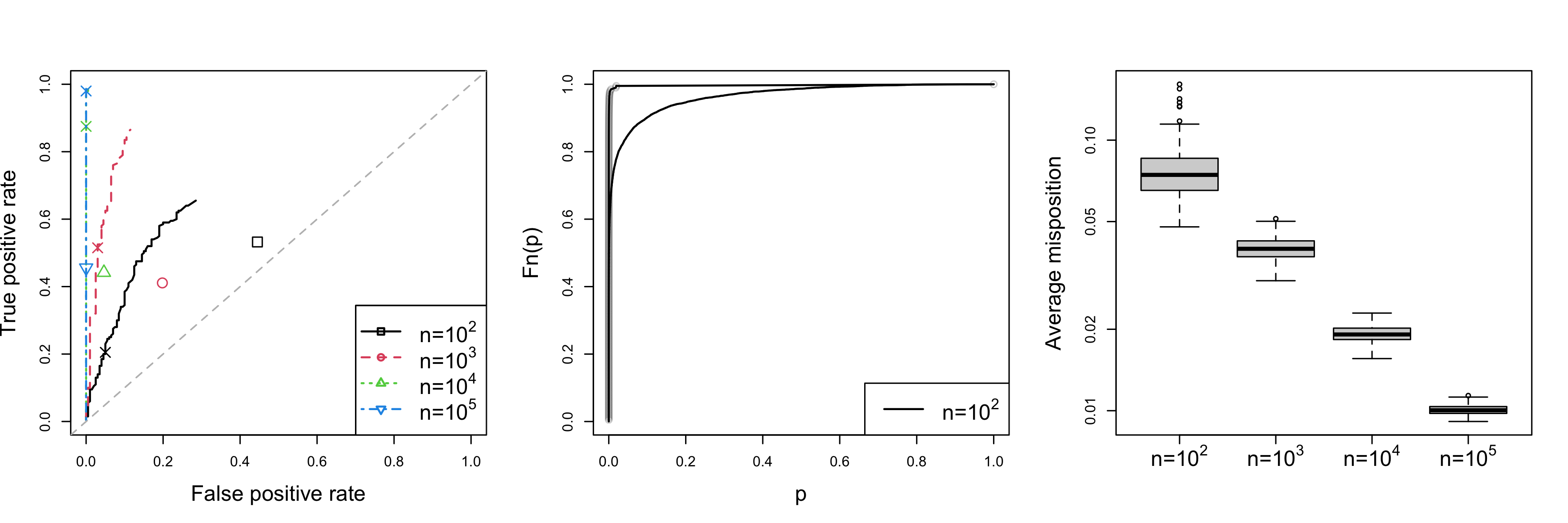
Figure 5: The results are based on $200$ simulation runs. On the left: False positive rate versus true positive rate obtained with Algorithm 3 adjusted to LSNM for varying $\tilde{\alpha}$ and $\alpha=0.05$. The crosses correspond to $\tilde{\alpha}=0.01$. The other symbols describe the performance of Algorithm 2 adjusted to LSNM. In the middle: empirical cumulative distribution function of the p-values obtained with HSIC. We compare the raw p-values from each split (lines only) to the cumulated p-value per simulation run (lines with dots). On the right: average misposition (12) of the estimated residuals with respect to the true residuals.

In Figure 5 we show the same performance metrics as in Figure 3. We see that our method can handle this toy example quite well. For $10^{5}$ samples, the performance with $\tilde{\alpha}=0.01$ is almost perfect, i.e., $196$ times the output is $\hat{W}=\mathopen{}\mathclose{{}\left\{2}\right\}$ and $4$ times $\hat{W}=\emptyset$. There are no false positives in $\hat{W}$.

The global test works well already for $10^{2}$ samples. After aggregation over the different splits, $H_{0}$ in (10) is rejected in every simulation run at $\alpha=0.05$. This can be facilitated by the fact that the fits are not good for this sample size such that there is more dependence on $\mathbf{x}$ for $\hat{\boldsymbol{\epsilon}}$ than for the true $\boldsymbol{\epsilon}$.

Finally, we compare how well the ordering of $\hat{\boldsymbol{\epsilon}}$ matches that of $\boldsymbol{\epsilon}$. For each run, we calculate the average misposition defined as

$$AMP=\dfrac{1}{n^{2}}\sum_{i=1}^{n}\mathopen{}\mathclose{{}\left|\sum_{l=1}^{n}\mathbbm{1}_{\mathopen{}\mathclose{{}\left\{\epsilon_{l}<\epsilon_{i}}\right\}}-\mathbbm{1}_{\mathopen{}\mathclose{{}\left\{\hat{\epsilon}_{l}<\hat{\epsilon}_{i}}\right\}}}\right|.$$ (12)

We show the according box plots on the right side of Figure 5. As desired, this quantity approaches $0$ for increasing sample size. For simplicity, we calculate this quantity only on a single split per simulation run.

7 Conclusion

In this paper, we introduce the notion of causal well-specification for additive noise models or their extension to heteroskedastic errors. Our viewpoint of local, i.e., for a subset of the covariates, causal well-specification, for which conditional independence between predictor and residual can serve as a proxy, provides a new option instead of rejecting entire models.

We present an algorithm to estimate our quantities of interest from finite data and provide some asymptotic guarantees. We demonstrate its application on simulation setups. This reveals some difficulties but also shows how considering multiple data splits can help even in hard cases.

Finally, we also apply our methodology and algorithm to regression problems extracted from a large-scale genomic dataset. While in many cases, causal well-specification appears to be not even approximately fulfilled, we find multiple examples where our estimate of well-specification is in line with an approximate validation from various gene knock down perturbations.

We want to emphasize that our formulation and analysis of what information conditional independence provides, which we present in Section 2, can also be used as stand-alone and other regression or machine learning methods for regression and assessing conditional dependence can be used.

Acknowledgement

The project leading to this application has received funding from the European Research Council (ERC) under the European Union’s Horizon 2020 research and innovation programme (grant agreement No 786461).
CS thanks Mathieu Chevalley for helpful discussions regarding finding use cases in the K562 dataset.

Appendix A Proofs

A.1 Proof of Theorem 1

Recall

$$Y\coloneqq\mathbb{E}\mathopen{}\mathclose{{}\left[Y|\mathbf{X}}\right]+\mathcal{E}$$

Due to (A2), we have

$$\mathbb{E}\mathopen{}\mathclose{{}\left[Y|\mathbf{X}}\right] =f_{\mathbf{X}_{U}Y}\mathopen{}\mathclose{{}\left(\mathbf{X}_{U},\mathbf{X}_{\text{PA}\mathopen{}\mathclose{{}\left(Y}\right)\setminus U}}\right)+\mathbb{E}\mathopen{}\mathclose{{}\left[f_{\mathbf{H}Y}\mathopen{}\mathclose{{}\left(\mathbf{H}_{\text{PA}\mathopen{}\mathclose{{}\left(Y}\right)},\mathbf{X}_{\text{PA}\mathopen{}\mathclose{{}\left(Y}\right)\setminus U}}\right)|\mathbf{X}}\right]\quad\text{such that}$$

$$\mathcal{E} =f_{\mathbf{H}Y}\mathopen{}\mathclose{{}\left(\mathbf{H}_{\text{PA}\mathopen{}\mathclose{{}\left(Y}\right)},\mathbf{X}_{\text{PA}\mathopen{}\mathclose{{}\left(Y}\right)\setminus U}}\right)-\mathbb{E}\mathopen{}\mathclose{{}\left[f_{\mathbf{H}Y}\mathopen{}\mathclose{{}\left(\mathbf{H}_{\text{PA}\mathopen{}\mathclose{{}\left(Y}\right)},\mathbf{X}_{\text{PA}\mathopen{}\mathclose{{}\left(Y}\right)\setminus U}}\right)|\mathbf{X}}\right].$$

Using (A1), $\mathbf{X}_{U}\perp\mathbf{H}_{\text{PA}\mathopen{}\mathclose{{}\left(Y}\right)}|\mathbf{X}_{-U}$, and trivially, $\mathbf{X}_{U}\perp\mathbf{X}_{-U}|\mathbf{X}_{-U}$. It follows

$$\mathbb{E}\mathopen{}\mathclose{{}\left[f_{\mathbf{H}Y}\mathopen{}\mathclose{{}\left(\mathbf{H}_{\text{PA}\mathopen{}\mathclose{{}\left(Y}\right)},\mathbf{X}_{\text{PA}\mathopen{}\mathclose{{}\left(Y}\right)\setminus U}}\right)|\mathbf{X}}\right]=\mathbb{E}\mathopen{}\mathclose{{}\left[f_{\mathbf{H}Y}\mathopen{}\mathclose{{}\left(\mathbf{H}_{\text{PA}\mathopen{}\mathclose{{}\left(Y}\right)},\mathbf{X}_{\text{PA}\mathopen{}\mathclose{{}\left(Y}\right)\setminus U}}\right)|\mathbf{X}_{-U}}\right] \perp\mathbf{X}_{U}|\mathbf{X}_{-U}\quad\text{and}$$

$$f_{\mathbf{H}Y}\mathopen{}\mathclose{{}\left(\mathbf{H}_{\text{PA}\mathopen{}\mathclose{{}\left(Y}\right)},\mathbf{X}_{\text{PA}\mathopen{}\mathclose{{}\left(Y}\right)\setminus j}}\right)\perp\mathbf{X}_{U}|\mathbf{X}_{-U}\quad\text{such that}\quad\mathcal{E} \perp\mathbf{X}_{U}|\mathbf{X}_{-U}.$$

Consider the counterfactual intervention. As $\mathbf{X}_{-U}$ remains unchanged, the second summand in (A2) could only change if $\mathbf{H}_{\text{PA}\mathopen{}\mathclose{{}\left(Y}\right)}$ changes. This could happen through some directed path from $\mathbf{X}_{U}$ to $\mathbf{H}_{\text{PA}\mathopen{}\mathclose{{}\left(Y}\right)}$ that is not blocked by $\mathbf{X}_{-U}$. By (A1), if such an effect from $\mathbf{X}_{U}$ to $\mathbf{H}_{\text{PA}\mathopen{}\mathclose{{}\left(Y}\right)}$ exists, it is constant for almost all $\mathbf{x}_{U}$. With (B1), we can extend this argument to all attainable $\mathbf{x}_{U}$. Hence, changing $\mathbf{X}_{U}$ from $\mathbf{x}_{U}$ to $\mathbf{x}^{\prime}_{U}$ while keeping $\mathbf{X}_{-U}$ fixed, cannot affect $\mathbf{H}_{\text{PA}\mathopen{}\mathclose{{}\left(Y}\right)}$ such that the second summand remains constant. For the first summand, we can directly plug in the counterfactual values of $\mathbf{X}$

In the conditional expectation given above only the first summand can change as the second is a function of only $\mathbf{X}_{-U}$. As the altered summand is the same for both $Y$ and $\mathbb{E}\mathopen{}\mathclose{{}\left[Y|\mathbf{X}}\right]$, the new value $y^{\prime}$ must exactly represent this change in conditional mean.

A.2 Proof of Theorem 2

Consider first the $\subseteq$-statement. This means that $H_{0,j}$ in (7) must hold $\forall j\in W$. Let $S=\mathopen{}\mathclose{{}\left\{1,\ldots,p}\right\}\setminus W$. Then, we want that

$$\mathcal{E}\perp\mathbf{X}_{W}|\mathbf{X}_{S}\implies\mathcal{E}\perp X_{j}|\mathbf{X}_{-j}.$$

This can be rewritten as

$$\mathcal{E}\perp\mathbf{X}_{W\setminus j},X_{j}|\mathbf{X}_{S}\implies\mathcal{E}\perp X_{j}|\mathbf{X}_{S},\mathbf{X}_{W\setminus j}.$$

This is the weak union property in Chapter 3 of Pearl, (1988) and hence holds for any random variables.

For $W=\tilde{W}$, we additionally need that $H_{0,j}$ cannot hold for any $j\in S$. By minimality of $S$

$$\mathcal{E}\not\perp X_{j},\mathbf{X}_{W}|\mathbf{X}_{S\setminus j}.$$

Then, the intersection property implies

$$\mathcal{E}\not\perp\mathbf{X}_{W}|X_{j},\mathbf{X}_{S\setminus j}\quad\text{or}\quad\mathcal{E}\not\perp X_{j}|\mathbf{X}_{W},\mathbf{X}_{S\setminus j}.$$

The first cannot hold by the definition of $W$, so the second must hold. This means that $H_{0,j}$ is not fulfilled, and $W=\tilde{W}$ is guaranteed.

A.3 Proof of Proposition 1

We have $T\mathopen{}\mathclose{{}\left(\cdot,\mathbf{X}_{U}}\right)=Q\mathopen{}\mathclose{{}\left(\cdot,\mathbf{X}_{U}}\right)/S\mathopen{}\mathclose{{}\left(\cdot}\right)$. As argued in (Azadkia and Chatterjee,, 2021) the denominator for unconditional independence tests is simply $1/6$ for continuous random variables. If $\mathcal{E}$ is conditionally continuously distributed, the same holds for its marginal distribution and thus also for the distribution of $\mathopen{}\mathclose{{}\left|\mathcal{E}}\right|$. Hence, it suffices to consider $Q\mathopen{}\mathclose{{}\left(\cdot,\mathbf{X}_{U}}\right)$ and the statement for $T\mathopen{}\mathclose{{}\left(\cdot,\mathbf{X}_{U}}\right)$ follows directly. Let $\mu$ and $\nu$ be the law of $\mathcal{E}$ and $\mathopen{}\mathclose{{}\left|\mathcal{E}}\right|$. Due to symmetry, it holds $d\nu\mathopen{}\mathclose{{}\left(t}\right)=2d\mu\mathopen{}\mathclose{{}\left(t}\right)\ \forall t\geq 0$.

$$Q\mathopen{}\mathclose{{}\left(\mathopen{}\mathclose{{}\left|\mathcal{E}}\right|,\mathbf{X}_{U}}\right)= \int_{0}^{\infty}\text{Var}\mathopen{}\mathclose{{}\left(\mathbb{P}\mathopen{}\mathclose{{}\left(\mathopen{}\mathclose{{}\left|\mathcal{E}}\right|\geq t|\mathbf{X}_{U}}\right)}\right)d\nu\mathopen{}\mathclose{{}\left(t}\right)=\int_{0}^{\infty}\text{Var}\mathopen{}\mathclose{{}\left(2\mathbb{P}\mathopen{}\mathclose{{}\left(\mathcal{E}\geq t|\mathbf{X}_{U}}\right)}\right)2d\mu\mathopen{}\mathclose{{}\left(t}\right)$$

$$=8 \int_{0}^{\infty}\text{Var}\mathopen{}\mathclose{{}\left(\mathbb{P}\mathopen{}\mathclose{{}\left(\mathcal{E}\geq t|\mathbf{X}_{U}}\right)}\right)d\mu\mathopen{}\mathclose{{}\left(t}\right)$$

$$\int_{-\infty}^{0}\text{Var}\mathopen{}\mathclose{{}\left(\mathbb{P}\mathopen{}\mathclose{{}\left(\mathcal{E}\geq t|\mathbf{X}_{U}}\right)}\right)d\mu\mathopen{}\mathclose{{}\left(t}\right)=\int_{-\infty}^{0}\text{Var}\mathopen{}\mathclose{{}\left(\mathbb{P}\mathopen{}\mathclose{{}\left(\mathcal{E}\leq-t|\mathbf{X}_{U}}\right)}\right)d\mu\mathopen{}\mathclose{{}\left(t}\right)$$

$$= \int_{-\infty}^{0}\text{Var}\mathopen{}\mathclose{{}\left(1-\mathbb{P}\mathopen{}\mathclose{{}\left(\mathcal{E}\geq-t|\mathbf{X}_{U}}\right)}\right)d\mu\mathopen{}\mathclose{{}\left(t}\right)=\int_{-\infty}^{0}\text{Var}\mathopen{}\mathclose{{}\left(\mathbb{P}\mathopen{}\mathclose{{}\left(\mathcal{E}\geq-t|\mathbf{X}_{U}}\right)}\right)d\mu\mathopen{}\mathclose{{}\left(t}\right)$$

$$\overset{t^{\prime}\leftarrow-t}{=} \int_{0}^{\infty}\text{Var}\mathopen{}\mathclose{{}\left(\mathbb{P}\mathopen{}\mathclose{{}\left(\mathcal{E}\geq t^{\prime}|\mathbf{X}_{U}}\right)}\right)d\mu\mathopen{}\mathclose{{}\left(t^{\prime}}\right)\ \text{such that}$$

$$Q\mathopen{}\mathclose{{}\left(\mathcal{E},\mathbf{X}_{U}}\right)= \int_{-\infty}^{\infty}\text{Var}\mathopen{}\mathclose{{}\left(\mathbb{P}\mathopen{}\mathclose{{}\left(\mathcal{E}\geq t|\mathbf{X}_{U}}\right)}\right)d\mu\mathopen{}\mathclose{{}\left(t}\right)=2\int_{0}^{\infty}\text{Var}\mathopen{}\mathclose{{}\left(\mathbb{P}\mathopen{}\mathclose{{}\left(\mathcal{E}\geq t|\mathbf{X}_{U}}\right)}\right)d\mu\mathopen{}\mathclose{{}\left(t}\right).$$

The first line uses symmetry, and the second chain of equalities uses symmetry as well as continuity to allow for a weak inequality in the complementary probability. Comparing the quantity on the first line to that on the last line we see that the ratio between the numerator terms is $4$.

A.4 Proof of Theorem 3

We build up the proof by some supporting Lemmata.

Lemma 1.

Assume (B3) and (B4).

$$\underset{n\rightarrow\infty}{\lim}\mathbb{P}\mathopen{}\mathclose{{}\left(\mathopen{}\mathclose{{}\left[g\mathopen{}\mathclose{{}\left(\epsilon_{i}}\right)>g\mathopen{}\mathclose{{}\left(\epsilon_{l}}\right)\cap g\mathopen{}\mathclose{{}\left(\hat{\epsilon}_{i}}\right)\leq g\mathopen{}\mathclose{{}\left(\hat{\epsilon}_{l}}\right)}\right]\cup\mathopen{}\mathclose{{}\left[g\mathopen{}\mathclose{{}\left(\epsilon_{i}}\right)<g\mathopen{}\mathclose{{}\left(\epsilon_{l}}\right)\cap g\mathopen{}\mathclose{{}\left(\hat{\epsilon}_{i}}\right)\geq g\mathopen{}\mathclose{{}\left(\hat{\epsilon}_{l}}\right)}\right]\cup\mathopen{}\mathclose{{}\left[g\mathopen{}\mathclose{{}\left(\epsilon_{i}}\right)=g\mathopen{}\mathclose{{}\left(\epsilon_{l}}\right)}\right]}\right)=0\ \forall i\neq l,$$

i.e., the probability that the estimates imply a different ordering between $i$ and $l$ approaches $0$.

Define $Q_{n}\mathopen{}\mathclose{{}\left(\cdot}\right)$ and $S_{n}\mathopen{}\mathclose{{}\left(\cdot}\right)$ as in Section 9 of Azadkia and Chatterjee, (2021).

Lemma 2.

Assume the conditions of Lemma 1. Let $U$ be any non-empty subset of $\mathopen{}\mathclose{{}\left\{1,\ldots,p}\right\}$. Then,

$$\underset{n\rightarrow\infty}{\lim} \mathbb{E}\mathopen{}\mathclose{{}\left[\mathopen{}\mathclose{{}\left|Q_{n}\mathopen{}\mathclose{{}\left(g\mathopen{}\mathclose{{}\left(\boldsymbol{\epsilon}}\right),\mathbf{x}_{U}}\right)-Q_{n}\mathopen{}\mathclose{{}\left(g\mathopen{}\mathclose{{}\left(\hat{\boldsymbol{\epsilon}}}\right),\mathbf{x}_{U}}\right)}\right|}\right]=0,\ \underset{n\rightarrow\infty}{\lim}\mathbb{E}\mathopen{}\mathclose{{}\left[\mathopen{}\mathclose{{}\left|S_{n}\mathopen{}\mathclose{{}\left(g\mathopen{}\mathclose{{}\left(\boldsymbol{\epsilon}}\right),\mathbf{x}_{U}}\right)-S_{n}\mathopen{}\mathclose{{}\left(g\mathopen{}\mathclose{{}\left(\hat{\boldsymbol{\epsilon}}}\right),\mathbf{x}_{U}}\right)}\right|}\right]=0$$

$$\underset{n\rightarrow\infty}{\lim} \mathbb{E}\mathopen{}\mathclose{{}\left[\mathopen{}\mathclose{{}\left|S_{n}\mathopen{}\mathclose{{}\left(g\mathopen{}\mathclose{{}\left(\boldsymbol{\epsilon}}\right)}\right)-S_{n}\mathopen{}\mathclose{{}\left(g\mathopen{}\mathclose{{}\left(\hat{\boldsymbol{\epsilon}}}\right)}\right)}\right|}\right]=0.$$

As in the sample splitting case $\mathopen{}\mathclose{{}\left(g\mathopen{}\mathclose{{}\left(\hat{\boldsymbol{\epsilon}}}\right),\mathbf{x}_{U}}\right)$ are i.i.d. copies, one can apply Lemma 11.9 in Azadkia and Chatterjee, (2021) to those. This yields

$$\mathbb{P}\mathopen{}\mathclose{{}\left(\mathopen{}\mathclose{{}\left|Q_{n}\mathopen{}\mathclose{{}\left(g\mathopen{}\mathclose{{}\left(\hat{\boldsymbol{\epsilon}}}\right),\mathbf{x}_{U}}\right)-\mathbb{E}\mathopen{}\mathclose{{}\left[Q_{n}\mathopen{}\mathclose{{}\left(g\mathopen{}\mathclose{{}\left(\hat{\boldsymbol{\epsilon}}}\right),\mathbf{x}_{U}}\right)}\right]}\right|\geq t}\right)\leq K_{1}\exp\mathopen{}\mathclose{{}\left(-K_{2}nt^{2}}\right),$$ (13)

for some positive $K_{1}$, $K_{2}$. Therefore, we can draw similar conclusions as in their Lemma 14.2.

Lemma 3.

Let $U$ be a subset of size $u$. Assume conditions (A1), which defines $\beta$, and (A2) from Azadkia and Chatterjee, (2021) for the data $\mathopen{}\mathclose{{}\left(g\mathopen{}\mathclose{{}\left(\mathcal{E}}\right),\mathbf{X}_{U}}\right)$ as well as conditions (B3) - (B4). Then, there exist positive $K_{1}$, $K_{2}$, and $K_{3}$ that do not depend on the sample size such that in the sample splitting case

$$\mathbb{P}\mathopen{}\mathclose{{}\left(\mathopen{}\mathclose{{}\left|Q_{n}\mathopen{}\mathclose{{}\left(g\mathopen{}\mathclose{{}\left(\hat{\boldsymbol{\epsilon}}}\right),\mathbf{x}_{U}}\right)-Q\mathopen{}\mathclose{{}\left(g\mathopen{}\mathclose{{}\left(\mathcal{E}}\right),\mathbf{X}_{U}}\right)}\right|\geq K_{1}\max\mathopen{}\mathclose{{}\left\{D^{1/3}\mathopen{}\mathclose{{}\left(n}\right),n^{-\min\mathopen{}\mathclose{{}\left\{-1/u,-1/2}\right\}}\log\mathopen{}\mathclose{{}\left(n}\right)^{u+\beta+1}}\right\}+t}\right)\leq$$

$$K_{2}\exp\mathopen{}\mathclose{{}\left(-K_{3}nt^{2}}\right)$$

Under (B2) and (B5) any set $U$ that is not a (weak) superset of $\mathopen{}\mathclose{{}\left\{1,\ldots,p}\right\}\setminus W$ cannot be sufficient for $g\mathopen{}\mathclose{{}\left(\mathcal{E}}\right)$. Thus, it suffices to bound the probability of $\hat{S}$ not being sufficient, and then Theorem 3 follows. This corresponds to Theorem 6.1 in Azadkia and Chatterjee, (2021). The only part of its proof that needs adaptation is Lemma 16.3. To proof an according result based on our Lemma 3, we require

$$L_{1}\max\mathopen{}\mathclose{{}\left\{D\mathopen{}\mathclose{{}\left(n}\right),n^{-\min\mathopen{}\mathclose{{}\left\{-1/K,-1/2}\right\}}\log\mathopen{}\mathclose{{}\left(n}\right)^{K+\beta+1}}\right\}\leq\dfrac{\delta}{16}.$$

Here, we use their definition of $\delta$, i.e., $\delta$ is the largest number such that for any insufficient subset $U\not\supseteq\mathopen{}\mathclose{{}\left(\mathopen{}\mathclose{{}\left\{1,\ldots,p}\right\}\setminus W}\right)$, there exists $j\not\in U$ that fulfils $Q\mathopen{}\mathclose{{}\left(g\mathopen{}\mathclose{{}\left(\mathcal{E}}\right),\mathbf{X}_{U\cup j}}\right)\geq Q\mathopen{}\mathclose{{}\left(g\mathopen{}\mathclose{{}\left(\mathcal{E}}\right),\mathbf{X}_{U}}\right)+\delta$. $K$ is the integer part of $1/\delta+2$. As we consider fixed data generating mechanisms, $\delta>0$ holds by construction. Hence, we do not mention it in the theorems explicitly. This inequality might require larger sample size than in Azadkia and Chatterjee, (2021) and larger $L_{6}$ accordingly. Apart from that, the proof follows from the same principles.

A.4.1 Proof of Lemma 1

The properties of $g\mathopen{}\mathclose{{}\left(\cdot}\right)$ imply that $g\mathopen{}\mathclose{{}\left(\mathcal{E}}\right)$ is a continuous random variable as well such that the probability of the last event has probability $0$ regardless of the sample size. As $i$ and $l$ are interchangeable, the first two events have the same probability and it suffices to analyse one. Let $\eta>0$ be arbitrary.

$$\mathbb{P}\mathopen{}\mathclose{{}\left(g\mathopen{}\mathclose{{}\left(\epsilon_{i}}\right)>g\mathopen{}\mathclose{{}\left(\epsilon_{l}}\right)\cap g\mathopen{}\mathclose{{}\left(\hat{\epsilon}_{i}}\right)\leq g\mathopen{}\mathclose{{}\left(\hat{\epsilon}_{l}}\right)}\right)=$$

$$\mathbb{P}\mathopen{}\mathclose{{}\left(g\mathopen{}\mathclose{{}\left(\epsilon_{i}}\right)>g\mathopen{}\mathclose{{}\left(\epsilon_{l}}\right)\cap g\mathopen{}\mathclose{{}\left(\hat{\epsilon}_{i}}\right)\leq g\mathopen{}\mathclose{{}\left(\hat{\epsilon}_{l}}\right)\cap g\mathopen{}\mathclose{{}\left(\epsilon_{i}}\right)-g\mathopen{}\mathclose{{}\left(\epsilon_{l}}\right)\leq\eta}\right)+$$

$$\mathbb{P}\mathopen{}\mathclose{{}\left(g\mathopen{}\mathclose{{}\left(\epsilon_{i}}\right)>g\mathopen{}\mathclose{{}\left(\epsilon_{l}}\right)\cap g\mathopen{}\mathclose{{}\left(\hat{\epsilon}_{i}}\right)\leq g\mathopen{}\mathclose{{}\left(\hat{\epsilon}_{l}}\right)\cap g\mathopen{}\mathclose{{}\left(\epsilon_{i}}\right)-g\mathopen{}\mathclose{{}\left(\epsilon_{l}}\right)>\eta}\right)\leq$$

$$\mathbb{P}\mathopen{}\mathclose{{}\left(\mathopen{}\mathclose{{}\left|g\mathopen{}\mathclose{{}\left(\epsilon_{i}}\right)-g\mathopen{}\mathclose{{}\left(\epsilon_{l}}\right)}\right|\leq\eta}\right)+\mathbb{P}\mathopen{}\mathclose{{}\left(\mathopen{}\mathclose{{}\left|g\mathopen{}\mathclose{{}\left(\hat{\epsilon}_{i}}\right)-g\mathopen{}\mathclose{{}\left(\epsilon_{i}}\right)}\right|+\mathopen{}\mathclose{{}\left|g\mathopen{}\mathclose{{}\left(\hat{\epsilon}_{l}}\right)-g\mathopen{}\mathclose{{}\left(\epsilon_{l}}\right)}\right|>\eta}\right)\leq$$

$$\mathbb{P}\mathopen{}\mathclose{{}\left(\mathopen{}\mathclose{{}\left|g\mathopen{}\mathclose{{}\left(\epsilon_{i}}\right)-g\mathopen{}\mathclose{{}\left(\epsilon_{l}}\right)}\right|\leq\eta}\right)+\mathbb{P}\mathopen{}\mathclose{{}\left(\max\mathopen{}\mathclose{{}\left\{\mathopen{}\mathclose{{}\left|g\mathopen{}\mathclose{{}\left(\hat{\epsilon}_{i}}\right)-g\mathopen{}\mathclose{{}\left(\epsilon_{i}}\right)}\right|,\mathopen{}\mathclose{{}\left|g\mathopen{}\mathclose{{}\left(\hat{\epsilon}_{l}}\right)-g\mathopen{}\mathclose{{}\left(\epsilon_{l}}\right)}\right|}\right\}>\eta/2}\right)\leq$$

$$\mathbb{P}\mathopen{}\mathclose{{}\left(\mathopen{}\mathclose{{}\left|g\mathopen{}\mathclose{{}\left(\epsilon_{i}}\right)-g\mathopen{}\mathclose{{}\left(\epsilon_{l}}\right)}\right|\leq\eta}\right)+2\mathbb{P}\mathopen{}\mathclose{{}\left(\mathopen{}\mathclose{{}\left|g\mathopen{}\mathclose{{}\left(\hat{\epsilon}_{i}}\right)-g\mathopen{}\mathclose{{}\left(\epsilon_{i}}\right)}\right|>\eta/2}\right)\leq\mathbb{P}\mathopen{}\mathclose{{}\left(\mathopen{}\mathclose{{}\left|g\mathopen{}\mathclose{{}\left(\epsilon_{i}}\right)-g\mathopen{}\mathclose{{}\left(\epsilon_{l}}\right)}\right|\leq\eta}\right)+2\mathbb{P}\mathopen{}\mathclose{{}\left(\mathopen{}\mathclose{{}\left|\hat{\epsilon}_{i}-\epsilon_{i}}\right|>\eta/2l}\right)$$

Let now $\eta$ depend on $n$. For $\eta\rightarrow 0$ the first term vanishes. If it approaches $0$ slowly enough, the second term vanishes as well assuming the regression is suitable. Thus, one can choose $\eta$ such that both terms vanish. Since the inequality holds for arbitrary $\eta$, the probability goes to $0$, i.e.,

$$\mathbb{P}\mathopen{}\mathclose{{}\left(\mathopen{}\mathclose{{}\left[g\mathopen{}\mathclose{{}\left(\epsilon_{l}}\right)\leq g\mathopen{}\mathclose{{}\left(\epsilon_{i}}\right)\cap g\mathopen{}\mathclose{{}\left(\hat{\epsilon}_{l}}\right)>g\mathopen{}\mathclose{{}\left(\hat{\epsilon}_{i}}\right)}\right]\cup\mathopen{}\mathclose{{}\left[g\mathopen{}\mathclose{{}\left(\epsilon_{l}}\right)\geq g\mathopen{}\mathclose{{}\left(\epsilon_{i}}\right)\cap g\mathopen{}\mathclose{{}\left(\hat{\epsilon}_{l}}\right)<g\mathopen{}\mathclose{{}\left(\hat{\epsilon}_{i}}\right)}\right]}\right)={\scriptstyle\mathcal{O}}\mathopen{}\mathclose{{}\left(1}\right).$$

A.4.2 Proof of Lemma 2

Let $R_{i}=\sum g\mathopen{}\mathclose{{}\left(\epsilon_{l}}\right)\leq g\mathopen{}\mathclose{{}\left(\epsilon_{i}}\right)$, $L_{i}=\sum g\mathopen{}\mathclose{{}\left(\epsilon_{l}}\right)\geq g\mathopen{}\mathclose{{}\left(\epsilon_{i}}\right)$, and $\hat{R}_{i}$, $\hat{L}_{i}$ the according quantities estimated with $\hat{\boldsymbol{\epsilon}}$. Note that index $M\mathopen{}\mathclose{{}\left(i}\right)$, i.e., the nearest neighbour of $i$ with respect to $\mathbf{x}_{U}$, only depends on observed quantities. Hence, it is the same for the estimated quantity $\hat{R}_{M\mathopen{}\mathclose{{}\left(i}\right)}$.

$$\mathopen{}\mathclose{{}\left|Q_{n}\mathopen{}\mathclose{{}\left(g\mathopen{}\mathclose{{}\left(\boldsymbol{\epsilon}}\right),\mathbf{x}_{U}}\right)-Q_{n}\mathopen{}\mathclose{{}\left(g\mathopen{}\mathclose{{}\left(\hat{\boldsymbol{\epsilon}}}\right),\mathbf{x}_{U}}\right)}\right|=\mathopen{}\mathclose{{}\left|\dfrac{1}{n^{2}}\sum_{i=1}^{n}\min\mathopen{}\mathclose{{}\left\{R_{i},R_{M\mathopen{}\mathclose{{}\left(i}\right)}}\right\}-\min\mathopen{}\mathclose{{}\left\{\hat{R}_{i},\hat{R}_{M\mathopen{}\mathclose{{}\left(i}\right)}}\right\}+\dfrac{\hat{L}_{i}^{2}-L_{i}^{2}}{n}}\right|\leq$$

$$\mathopen{}\mathclose{{}\left|\dfrac{1}{n^{2}}\sum_{i=1}^{n}\min\mathopen{}\mathclose{{}\left\{R_{i},R_{M\mathopen{}\mathclose{{}\left(i}\right)}}\right\}-\min\mathopen{}\mathclose{{}\left\{\hat{R}_{i},\hat{R}_{M\mathopen{}\mathclose{{}\left(i}\right)}}\right\}}\right|+\mathopen{}\mathclose{{}\left|\dfrac{1}{n^{3}}\sum_{i=1}^{n}\hat{L}_{i}^{2}-L_{i}^{2}}\right|$$

$$\mathopen{}\mathclose{{}\left|S_{n}\mathopen{}\mathclose{{}\left(g\mathopen{}\mathclose{{}\left(\boldsymbol{\epsilon}}\right),\mathbf{x}_{U}}\right)-S_{n}\mathopen{}\mathclose{{}\left(g\mathopen{}\mathclose{{}\left(\hat{\boldsymbol{\epsilon}}}\right),\mathbf{x}_{U}}\right)}\right|=\mathopen{}\mathclose{{}\left|\dfrac{1}{n^{2}}\sum_{i=1}^{n}R_{i}-\hat{R}_{i}+\min\mathopen{}\mathclose{{}\left\{\hat{R}_{i},\hat{R}_{M\mathopen{}\mathclose{{}\left(i}\right)}}\right\}-\min\mathopen{}\mathclose{{}\left\{R_{i},R_{M\mathopen{}\mathclose{{}\left(i}\right)}}\right\}}\right|\leq$$

$$\mathopen{}\mathclose{{}\left|\dfrac{1}{n^{2}}\sum_{i=1}^{n}R_{i}-\hat{R}_{i}}\right|+\mathopen{}\mathclose{{}\left|\dfrac{1}{n^{2}}\sum_{i=1}^{n}\min\mathopen{}\mathclose{{}\left\{\hat{R}_{i},\hat{R}_{M\mathopen{}\mathclose{{}\left(i}\right)}}\right\}-\min\mathopen{}\mathclose{{}\left\{R_{i},R_{M\mathopen{}\mathclose{{}\left(i}\right)}}\right\}}\right|$$

$$\mathopen{}\mathclose{{}\left|S_{n}\mathopen{}\mathclose{{}\left(g\mathopen{}\mathclose{{}\left(\boldsymbol{\epsilon}}\right)}\right)-S_{n}\mathopen{}\mathclose{{}\left(g\mathopen{}\mathclose{{}\left(\hat{\boldsymbol{\epsilon}}}\right)}\right)}\right|=\mathopen{}\mathclose{{}\left|\dfrac{1}{n^{3}}\sum_{i=1}^{n}n\mathopen{}\mathclose{{}\left(L_{i}-\hat{L}_{i}}\right)+\hat{L}_{i}^{2}-L_{i}^{2}}\right|\leq\mathopen{}\mathclose{{}\left|\dfrac{1}{n^{2}}\sum_{i=1}^{n}L_{i}-\hat{L}_{i}}\right|+\mathopen{}\mathclose{{}\left|\dfrac{1}{n^{3}}\sum_{i=1}^{n}\hat{L}_{i}^{2}-L_{i}^{2}}\right|$$

Thus, there are four different terms to be controlled. If both $\boldsymbol{\epsilon}$ and $\hat{\boldsymbol{\epsilon}}$ have $n$ distinct values, all the terms that do not depend on the nearest neighbouring property amongst $\mathbf{x}_{U}$ are trivially $0$ for every sample sizes. However, we can prove convergence without this assumption.

$$\mathbb{E}\mathopen{}\mathclose{{}\left[\mathopen{}\mathclose{{}\left|\dfrac{1}{n^{2}}\sum_{i=1}^{n}R_{i}-\hat{R}_{i}}\right|}\right]\leq\mathbb{E}\mathopen{}\mathclose{{}\left[\dfrac{1}{n^{2}}\sum_{i=1}^{n}\mathopen{}\mathclose{{}\left|R_{i}-\hat{R}_{i}}\right|}\right]=\mathbb{E}\mathopen{}\mathclose{{}\left[\dfrac{1}{n^{2}}\sum_{i=1}^{n}\mathopen{}\mathclose{{}\left|\sum_{l=1}^{n}\mathbbm{1}_{\mathopen{}\mathclose{{}\left\{g\mathopen{}\mathclose{{}\left(\epsilon_{l}}\right)\leq g\mathopen{}\mathclose{{}\left(\epsilon_{i}}\right)}\right\}}-\mathbbm{1}_{\mathopen{}\mathclose{{}\left\{g\mathopen{}\mathclose{{}\left(\hat{\epsilon}_{l}}\right)\leq g\mathopen{}\mathclose{{}\left(\hat{\epsilon}_{i}}\right)}\right\}}}\right|}\right]=$$

$$\mathbb{E}\mathopen{}\mathclose{{}\left[\dfrac{1}{n^{2}}\sum_{i=1}^{n}\mathopen{}\mathclose{{}\left|\sum_{l\neq i}\mathbbm{1}_{\mathopen{}\mathclose{{}\left\{g\mathopen{}\mathclose{{}\left(\epsilon_{l}}\right)\leq g\mathopen{}\mathclose{{}\left(\epsilon_{i}}\right)}\right\}}-\mathbbm{1}_{\mathopen{}\mathclose{{}\left\{g\mathopen{}\mathclose{{}\left(\hat{\epsilon}_{l}}\right)\leq g\mathopen{}\mathclose{{}\left(\hat{\epsilon}_{i}}\right)}\right\}}}\right|}\right]\leq\dfrac{1}{n^{2}}\sum_{i=1}^{n}\sum_{l\neq i}\mathbb{E}\mathopen{}\mathclose{{}\left[\mathopen{}\mathclose{{}\left|\mathbbm{1}_{\mathopen{}\mathclose{{}\left\{g\mathopen{}\mathclose{{}\left(\epsilon_{l}}\right)\leq g\mathopen{}\mathclose{{}\left(\epsilon_{i}}\right)}\right\}}-\mathbbm{1}_{\mathopen{}\mathclose{{}\left\{g\mathopen{}\mathclose{{}\left(\hat{\epsilon}_{l}}\right)\leq g\mathopen{}\mathclose{{}\left(\hat{\epsilon}_{i}}\right)}\right\}}}\right|}\right]=$$

$$\dfrac{n^{2}-n}{n^{2}}\mathbb{E}\mathopen{}\mathclose{{}\left[\mathopen{}\mathclose{{}\left|\mathbbm{1}_{\mathopen{}\mathclose{{}\left\{g\mathopen{}\mathclose{{}\left(\epsilon_{l}}\right)\leq g\mathopen{}\mathclose{{}\left(\epsilon_{i}}\right)}\right\}}-\mathbbm{1}_{\mathopen{}\mathclose{{}\left\{g\mathopen{}\mathclose{{}\left(\hat{\epsilon}_{l}}\right)\leq g\mathopen{}\mathclose{{}\left(\hat{\epsilon}_{i}}\right)}\right\}}}\right|}\right]=$$

$$\dfrac{n^{2}-n}{n^{2}}\mathbb{P}\mathopen{}\mathclose{{}\left(\mathopen{}\mathclose{{}\left[g\mathopen{}\mathclose{{}\left(\epsilon_{l}}\right)\leq g\mathopen{}\mathclose{{}\left(\epsilon_{i}}\right)\cap g\mathopen{}\mathclose{{}\left(\hat{\epsilon}_{l}}\right)>g\mathopen{}\mathclose{{}\left(\hat{\epsilon}_{i}}\right)}\right]\cup\mathopen{}\mathclose{{}\left[g\mathopen{}\mathclose{{}\left(\epsilon_{l}}\right)\geq g\mathopen{}\mathclose{{}\left(\epsilon_{i}}\right)\cap g\mathopen{}\mathclose{{}\left(\hat{\epsilon}_{l}}\right)<g\mathopen{}\mathclose{{}\left(\hat{\epsilon}_{i}}\right)}\right]}\right)\overset{n\rightarrow\infty}{\rightarrow}0$$

by Lemma 1. In the last two expressions, $l\neq i$ is assumed. The argument for the term with $L_{i}-\hat{L}_{i}$ is identical.

$$\mathbb{E}\mathopen{}\mathclose{{}\left[\mathopen{}\mathclose{{}\left|\dfrac{1}{n^{2}}\sum_{i=1}^{n}\min\mathopen{}\mathclose{{}\left\{\hat{R}_{i},\hat{R}_{M\mathopen{}\mathclose{{}\left(i}\right)}}\right\}-\min\mathopen{}\mathclose{{}\left\{R_{i},R_{M\mathopen{}\mathclose{{}\left(i}\right)}}\right\}}\right|\leq\mathbb{E}\mathopen{}\mathclose{{}\left[\dfrac{1}{n^{2}}\sum_{i=1}^{n}\mathopen{}\mathclose{{}\left|\hat{R}_{i}-R_{i}}\right|+\mathopen{}\mathclose{{}\left|\hat{R}_{M\mathopen{}\mathclose{{}\left(i}\right)}-R_{M\mathopen{}\mathclose{{}\left(i}\right)}}\right|}\right]}\right]=$$

$$\mathbb{E}\mathopen{}\mathclose{{}\left[\dfrac{1}{n^{2}}\sum_{i=1}^{n}\mathopen{}\mathclose{{}\left|\hat{R}_{i}-R_{i}}\right|+\dfrac{1}{n^{2}}\sum_{i=1}^{n}\sum_{l:\ M\mathopen{}\mathclose{{}\left(l}\right)=i}\mathopen{}\mathclose{{}\left|\hat{R}_{i}-R_{i}}\right|}\right]=\mathbb{E}\mathopen{}\mathclose{{}\left[\dfrac{1}{n^{2}}\sum_{i=1}^{n}\mathopen{}\mathclose{{}\left|\hat{R}_{i}-R_{i}}\right|\mathopen{}\mathclose{{}\left(1+\sum_{l\neq i}\mathbbm{1}_{M\mathopen{}\mathclose{{}\left(l}\right)=i}}\right)}\right]=$$

$$\dfrac{1}{n^{2}}\sum_{i=1}^{n}\mathbb{E}\mathopen{}\mathclose{{}\left[\mathopen{}\mathclose{{}\left|\hat{R}_{i}-R_{i}}\right|\mathopen{}\mathclose{{}\left(1+\sum_{l\neq i}\mathbbm{1}_{M\mathopen{}\mathclose{{}\left(l}\right)=i}}\right)}\right]=\dfrac{1}{n^{2}}\sum_{i=1}^{n}\mathbb{E}\mathopen{}\mathclose{{}\left[\mathopen{}\mathclose{{}\left|\hat{R}_{i}-R_{i}}\right|\mathbb{E}\mathopen{}\mathclose{{}\left[1+\sum_{l\neq i}\mathbbm{1}_{M\mathopen{}\mathclose{{}\left(l}\right)=i}|\hat{R}_{i},R_{i}}\right]}\right]\leq$$

$$\dfrac{2+C\mathopen{}\mathclose{{}\left(p}\right)}{n^{2}}\sum_{i=1}^{n}\mathbb{E}\mathopen{}\mathclose{{}\left[\mathopen{}\mathclose{{}\left|\hat{R}_{i}-R_{i}}\right|}\right]\overset{n\rightarrow\infty}{\rightarrow}0.$$

By Lemma 11.4 in Azadkia and Chatterjee, (2021), there is a dimension dependent constant such that no point can be the nearest neighbour of more than $C\mathopen{}\mathclose{{}\left(p}\right)$ distinct points in $\mathbb{R}^{p}$. If there are $l$ such that $\mathbf{x}_{l,U}=\mathbf{x}_{i,U}$, $M\mathopen{}\mathclose{{}\left(l}\right)$ is chosen uniformly at random from this set, and in expectation there is one $l$ such that $M\mathopen{}\mathclose{{}\left(l}\right)=i$. As this uniform draw is independent of $R_{i}$ and $\hat{R}_{i}$, the upper bound also applies to the conditional expectation and we can pull it out.

$$\mathbb{E}\mathopen{}\mathclose{{}\left[\mathopen{}\mathclose{{}\left|\dfrac{1}{n^{3}}\sum_{i=1}^{n}L_{i}^{2}-\hat{L}_{i}^{2}}\right|}\right]=\mathbb{E}\mathopen{}\mathclose{{}\left[\mathopen{}\mathclose{{}\left|\dfrac{1}{n^{3}}\sum_{i=1}^{n}\mathopen{}\mathclose{{}\left(L_{i}-\hat{L}_{i}}\right)\mathopen{}\mathclose{{}\left(L_{i}+\hat{L}_{i}}\right)}\right|}\right]\leq\mathbb{E}\mathopen{}\mathclose{{}\left[\mathopen{}\mathclose{{}\left|\dfrac{2}{n^{2}}\sum_{i=1}^{n}L_{i}-\hat{L}_{i}}\right|}\right]\overset{n\rightarrow\infty}{\rightarrow}0.$$

Thus, every term is under control which concludes the proof. As all the terms are at most of the same order as the probability in Lemma 1, the bound on the convergence rate follows directly.

A.4.3 Proof of Lemma 3

By Lemma 2, there exists a rate, say, $D\mathopen{}\mathclose{{}\left(n}\right)={\scriptstyle\mathcal{O}}\mathopen{}\mathclose{{}\left(1}\right)$ such that

$$\mathopen{}\mathclose{{}\left|\mathbb{E}\mathopen{}\mathclose{{}\left[Q_{n}\mathopen{}\mathclose{{}\left(g\mathopen{}\mathclose{{}\left(\hat{\boldsymbol{\epsilon}}}\right),\mathbf{x}_{U}}\right)}\right]-\mathbb{E}\mathopen{}\mathclose{{}\left[Q_{n}\mathopen{}\mathclose{{}\left(g\mathopen{}\mathclose{{}\left(\epsilon}\right),\mathbf{x}_{U}}\right)}\right]}\right|=\mathcal{O}\mathopen{}\mathclose{{}\left(D\mathopen{}\mathclose{{}\left(n}\right)}\right).$$

Then,

$$\mathopen{}\mathclose{{}\left|Q_{n}\mathopen{}\mathclose{{}\left(g\mathopen{}\mathclose{{}\left(\hat{\boldsymbol{\epsilon}}}\right),\mathbf{x}_{U}}\right)-Q\mathopen{}\mathclose{{}\left(g\mathopen{}\mathclose{{}\left(\mathcal{E}}\right),\mathbf{X}_{U}}\right)}\right|\leq$$

$$\mathopen{}\mathclose{{}\left|Q_{n}\mathopen{}\mathclose{{}\left(g\mathopen{}\mathclose{{}\left(\hat{\boldsymbol{\epsilon}}}\right),\mathbf{x}_{U}}\right)-\mathbb{E}\mathopen{}\mathclose{{}\left[Q_{n}\mathopen{}\mathclose{{}\left(g\mathopen{}\mathclose{{}\left(\hat{\boldsymbol{\epsilon}}}\right),\mathbf{x}_{U}}\right)}\right]}\right|+\mathopen{}\mathclose{{}\left|\mathbb{E}\mathopen{}\mathclose{{}\left[Q_{n}\mathopen{}\mathclose{{}\left(g\mathopen{}\mathclose{{}\left(\hat{\boldsymbol{\epsilon}}}\right),\mathbf{x}_{U}}\right)}\right]-\mathbb{E}\mathopen{}\mathclose{{}\left[Q_{n}\mathopen{}\mathclose{{}\left(g\mathopen{}\mathclose{{}\left(\epsilon}\right),\mathbf{x}_{U}}\right)}\right]}\right|+$$

$$\mathopen{}\mathclose{{}\left|\mathbb{E}\mathopen{}\mathclose{{}\left[Q_{n}\mathopen{}\mathclose{{}\left(g\mathopen{}\mathclose{{}\left(\epsilon}\right),\mathbf{x}_{U}}\right)-Q\mathopen{}\mathclose{{}\left(g\mathopen{}\mathclose{{}\left(\mathcal{E}}\right),\mathbf{X}_{U}}\right)}\right]}\right|\leq$$

$$\mathopen{}\mathclose{{}\left|Q_{n}\mathopen{}\mathclose{{}\left(g\mathopen{}\mathclose{{}\left(\hat{\boldsymbol{\epsilon}}}\right),\mathbf{x}_{U}}\right)-\mathbb{E}\mathopen{}\mathclose{{}\left[Q_{n}\mathopen{}\mathclose{{}\left(g\mathopen{}\mathclose{{}\left(\hat{\boldsymbol{\epsilon}}}\right),\mathbf{x}_{U}}\right)}\right]}\right|+K_{1}\max\mathopen{}\mathclose{{}\left\{D\mathopen{}\mathclose{{}\left(n}\right),n^{-\min\mathopen{}\mathclose{{}\left\{-1/u,-1/2}\right\}}\log\mathopen{}\mathclose{{}\left(n}\right)^{u+\beta+1}}\right\},$$

using the rate derived in Lemma 14.2 of (Azadkia and Chatterjee,, 2021). Therefore, with (13),

$$\mathbb{P}\mathopen{}\mathclose{{}\left(\mathopen{}\mathclose{{}\left|Q_{n}\mathopen{}\mathclose{{}\left(g\mathopen{}\mathclose{{}\left(\hat{\boldsymbol{\epsilon}}}\right),\mathbf{x}_{U}}\right)-Q\mathopen{}\mathclose{{}\left(g\mathopen{}\mathclose{{}\left(\mathcal{E}}\right),\mathbf{X}_{U}}\right)}\right|\geq K_{1}\max\mathopen{}\mathclose{{}\left\{D\mathopen{}\mathclose{{}\left(n}\right),n^{-\min\mathopen{}\mathclose{{}\left\{-1/u,-1/2}\right\}}\log\mathopen{}\mathclose{{}\left(n}\right)^{u+\beta+1}}\right\}+t}\right)\leq$$

$$\mathbb{P}\mathopen{}\mathclose{{}\left(\mathopen{}\mathclose{{}\left|Q_{n}\mathopen{}\mathclose{{}\left(g\mathopen{}\mathclose{{}\left(\hat{\boldsymbol{\epsilon}}}\right),\mathbf{x}_{U}}\right)-\mathbb{E}\mathopen{}\mathclose{{}\left[Q_{n}\mathopen{}\mathclose{{}\left(g\mathopen{}\mathclose{{}\left(\hat{\boldsymbol{\epsilon}}}\right),\mathbf{x}_{U}}\right)}\right]}\right|\geq t}\right)\leq K_{2}\exp\mathopen{}\mathclose{{}\left(-K_{3}nt^{2}}\right).$$

A.5 Proof of Theorem 4

Again, we only have to bound the probability of $\hat{S}$ not being sufficient.

Using Lemma 2 and the Markov inequality, we see

$$\mathbb{P}\mathopen{}\mathclose{{}\left(\mathopen{}\mathclose{{}\left|Q_{n}\mathopen{}\mathclose{{}\left(g\mathopen{}\mathclose{{}\left(\hat{\boldsymbol{\epsilon}}}\right),\mathbf{x}_{U}}\right)-Q_{n}\mathopen{}\mathclose{{}\left(g\mathopen{}\mathclose{{}\left(\boldsymbol{\epsilon}}\right),\mathbf{x}_{U}}\right)}\right|\geq t}\right)\leq\dfrac{K_{1}D\mathopen{}\mathclose{{}\left(n}\right)}{t}.$$

Hence, we get

$$\mathbb{P} \mathopen{}\mathclose{{}\left(\mathopen{}\mathclose{{}\left|Q_{n}\mathopen{}\mathclose{{}\left(g\mathopen{}\mathclose{{}\left(\hat{\boldsymbol{\epsilon}}}\right),\mathbf{x}_{U}}\right)-Q\mathopen{}\mathclose{{}\left(g\mathopen{}\mathclose{{}\left(\mathcal{E}}\right),\mathbf{X}_{U}}\right)}\right|\geq K_{1}n^{-\min\mathopen{}\mathclose{{}\left\{-1/u,-1/2}\right\}}\log\mathopen{}\mathclose{{}\left(n}\right)^{u+\beta+1}+t}\right)\leq$$

$$\mathbb{P} \Big{(}\mathopen{}\mathclose{{}\left|Q_{n}\mathopen{}\mathclose{{}\left(g\mathopen{}\mathclose{{}\left(\hat{\boldsymbol{\epsilon}}}\right),\mathbf{x}_{U}}\right)-Q_{n}\mathopen{}\mathclose{{}\left(g\mathopen{}\mathclose{{}\left(\boldsymbol{\epsilon}}\right),\mathbf{x}_{U}}\right)}\right|+\mathopen{}\mathclose{{}\left|Q_{n}\mathopen{}\mathclose{{}\left(g\mathopen{}\mathclose{{}\left(\boldsymbol{\epsilon}}\right),\mathbf{x}_{U}}\right)-Q\mathopen{}\mathclose{{}\left(g\mathopen{}\mathclose{{}\left(\mathcal{E}}\right),\mathbf{X}_{U}}\right)}\right|\geq$$

$$K_{1}n^{-\min\mathopen{}\mathclose{{}\left\{-1/u,-1/2}\right\}}\log\mathopen{}\mathclose{{}\left(n}\right)^{u+\beta+1}+t\Big{)}\leq$$

$$\mathbb{P} \mathopen{}\mathclose{{}\left(\mathopen{}\mathclose{{}\left|Q_{n}\mathopen{}\mathclose{{}\left(g\mathopen{}\mathclose{{}\left(\hat{\boldsymbol{\epsilon}}}\right),\mathbf{x}_{U}}\right)-Q_{n}\mathopen{}\mathclose{{}\left(g\mathopen{}\mathclose{{}\left(\boldsymbol{\epsilon}}\right),\mathbf{x}_{U}}\right)}\right|\geq\dfrac{t}{2}}\right)+$$

$$\mathbb{P} \mathopen{}\mathclose{{}\left(\mathopen{}\mathclose{{}\left|Q_{n}\mathopen{}\mathclose{{}\left(g\mathopen{}\mathclose{{}\left(\boldsymbol{\epsilon}}\right),\mathbf{x}_{U}}\right)-Q\mathopen{}\mathclose{{}\left(g\mathopen{}\mathclose{{}\left(\mathcal{E}}\right),\mathbf{X}_{U}}\right)}\right|\geq K_{1}n^{-\min\mathopen{}\mathclose{{}\left\{-1/u,-1/2}\right\}}\log\mathopen{}\mathclose{{}\left(n}\right)^{u+\beta+1}+\dfrac{t}{2}}\right)\leq$$

$$\dfrac{K_{2}\mathopen{}\mathclose{{}\left(n}\right)}{t}+K_{3}\exp\mathopen{}\mathclose{{}\left(-K_{4}nt^{2}}\right)\leq K_{5}\max\mathopen{}\mathclose{{}\left\{\dfrac{D\mathopen{}\mathclose{{}\left(n}\right)}{t},\exp\mathopen{}\mathclose{{}\left(-K_{4}nt^{2}}\right)}\right\},$$

where we used Lemma 14.2 in (Azadkia and Chatterjee,, 2021) in the second to last inequality. Finally, we can follow the proof idea of Lemma 16.3 in (Azadkia and Chatterjee,, 2021) with the given probability bound showing that the probability of $\hat{S}$ being insufficient goes to $0$.

A.6 Proof of Proposition 2

For the least squares parameter, we have

$$\hat{\beta}=\dfrac{\mathbf{x}^{\top}\mathbf{y}}{\mathbf{x}^{\top}\mathbf{x}}=\beta+\dfrac{\mathbf{x}^{\top}\boldsymbol{\epsilon}}{\mathbf{x}^{\top}\mathbf{x}},\qquad\mathbb{P}\mathopen{}\mathclose{{}\left(\hat{\beta}=\beta}\right)=\mathbb{P}\mathopen{}\mathclose{{}\left(\mathbf{x}^{\top}\boldsymbol{\epsilon}=0}\right)=0$$

since $X$ is a continuous random variable. However, for large enough sample size, it holds (with high probability)

$$i\in\underset{l}{\text{arg min}}\mathopen{}\mathclose{{}\left|\hat{\epsilon}_{i}-\epsilon_{l}}\right|\ \forall i,$$

i.e., the estimated residuals scatter closely around the true value from the discrete set. There are roughly $n/k$ observations per possible value of $\mathcal{E}$, and, due to the linear dependence, around each value, the ordering of $\hat{\boldsymbol{\epsilon}}$ corresponds to the ordering of $\mathbf{x}$ or is exactly inverted. Therefore,

$$\hat{R}_{i}\mod\dfrac{n}{k}\approx\hat{R}_{M\mathopen{}\mathclose{{}\left(i}\right)}\mod\dfrac{n}{k}\ \text{and}\ \hat{R}_{M\mathopen{}\mathclose{{}\left(i}\right)}|\hat{R}_{i}\dot{\sim}\hat{R}_{i}\mod\dfrac{n}{k}+\dfrac{n}{k}\text{Unif}\mathopen{}\mathclose{{}\left\{0,\ldots,k-1}\right\}.$$

Since the $\hat{\epsilon}_{i}$ all have distinct values, it holds

$$\sum_{i=1}^{n}\hat{L}_{i} =\sum_{i=1}^{n}i=\dfrac{n^{2}+n}{2}\ \text{and}\sum_{i=1}^{n}\hat{L}_{i}^{2}=\sum_{i=1}^{n}i^{2}=\dfrac{n\mathopen{}\mathclose{{}\left(n+1}\right)\mathopen{}\mathclose{{}\left(2n+1}\right)}{6}\ \text{such that}$$

$$T_{n}\mathopen{}\mathclose{{}\left(\hat{\boldsymbol{\epsilon}},\mathbf{x}}\right) =\dfrac{n\sum_{i=1}^{n}\min\mathopen{}\mathclose{{}\left\{\hat{R}_{i},\hat{R}_{M\mathopen{}\mathclose{{}\left(i}\right)}}\right\}-\dfrac{n\mathopen{}\mathclose{{}\left(n+1}\right)\mathopen{}\mathclose{{}\left(2n+1}\right)}{6}}{\dfrac{n^{3}+n^{2}}{2}-\dfrac{n\mathopen{}\mathclose{{}\left(n+1}\right)\mathopen{}\mathclose{{}\left(2n+1}\right)}{6}}.$$

We consider the only random term

$$\mathbb{E}\mathopen{}\mathclose{{}\left[\sum_{i=1}^{n}\min\mathopen{}\mathclose{{}\left\{\hat{R}_{i},\hat{R}_{M\mathopen{}\mathclose{{}\left(i}\right)}}\right\}}\right] =\mathbb{E}\mathopen{}\mathclose{{}\left[\sum_{\hat{R}_{i}=1}^{n}\min\mathopen{}\mathclose{{}\left\{\hat{R}_{i},\hat{R}_{M\mathopen{}\mathclose{{}\left(i}\right)}}\right\}}\right]=\mathbb{E}\mathopen{}\mathclose{{}\left[\sum_{\hat{R}_{i}=1}^{n}\min\mathopen{}\mathclose{{}\left\{\hat{R}_{i},\hat{R}_{M\mathopen{}\mathclose{{}\left(i}\right)}}\right\}|\hat{R}_{1},\ldots,\hat{R}_{n}}\right]$$

$$=\sum_{\hat{R}_{i}=1}^{n}\mathbb{E}\mathopen{}\mathclose{{}\left[\min\mathopen{}\mathclose{{}\left\{\hat{R}_{i},\hat{R}_{M\mathopen{}\mathclose{{}\left(i}\right)}}\right\}|\hat{R}_{1},\ldots,\hat{R}_{n}}\right]=\sum_{\hat{R}_{i}=1}^{n}\mathbb{E}\mathopen{}\mathclose{{}\left[\min\mathopen{}\mathclose{{}\left\{\hat{R}_{i},\hat{R}_{M\mathopen{}\mathclose{{}\left(i}\right)}}\right\}|\hat{R}_{i}}\right].$$

The first equality holds as summing over all $i$ is the same as summing over all ranks. As the problem is permutation invariant, conditioning on all ranks does not change the expectation. Under the conditioning, the ranks are deterministic and linearity of expectation applies. Finally, knowing any rank apart from $\hat{R}_{i}$ does not influence $\min\mathopen{}\mathclose{{}\left\{\hat{R}_{i},\hat{R}_{M\mathopen{}\mathclose{{}\left(i}\right)}}\right\}$. We analyse the expectation under the approximate conditional distribution as given above. If $\hat{R}_{i}\leq n/k$, $\min\mathopen{}\mathclose{{}\left\{\hat{R}_{i},\hat{R}_{M\mathopen{}\mathclose{{}\left(i}\right)}}\right\}=\hat{R}_{i}$. If $n/k<\hat{R}_{i}\leq 2n/k$ and the uniformly chosen number is $0$, $\min\mathopen{}\mathclose{{}\left\{\hat{R}_{i},\hat{R}_{M\mathopen{}\mathclose{{}\left(i}\right)}}\right\}=\hat{R}_{i}-n/k$. This has probability $1/k$. Otherwise, $\min\mathopen{}\mathclose{{}\left\{\hat{R}_{i},\hat{R}_{M\mathopen{}\mathclose{{}\left(i}\right)}}\right\}=\hat{R}_{i}$. Analogously, if $ln/k<\hat{R}_{i}\leq(l+1)n/k$ for some integer $0\leq l<k$, i.e., $l=\max\mathopen{}\mathclose{{}\left\{r\in\mathbb{N}_{0}|r<\hat{R}_{i}k/n}\right\}$, it holds under the approximate distribution

$$\tilde{\mathbb{E}}\mathopen{}\mathclose{{}\left[\min\mathopen{}\mathclose{{}\left\{\hat{R}_{i},\hat{R}_{M\mathopen{}\mathclose{{}\left(i}\right)}}\right\}|\hat{R}_{i}}\right]=\hat{R}_{i}-\dfrac{1}{k}\sum_{r=0}^{l}\dfrac{rn}{k}=\hat{R}_{i}-\dfrac{n}{2k^{2}}\mathopen{}\mathclose{{}\left(l^{2}+l}\right).$$

For each possible value of $l$, there are $n/k$ ranks such that $ln/k<\hat{R}_{i}\leq(l+1)n/k$. Therefore,

$$\sum_{\hat{R}_{i}=1}^{n}\tilde{\mathbb{E}}\mathopen{}\mathclose{{}\left[\min\mathopen{}\mathclose{{}\left\{\hat{R}_{i},\hat{R}_{M\mathopen{}\mathclose{{}\left(i}\right)}}\right\}|\hat{R}_{i}}\right]=\sum_{\hat{R}_{i}=1}^{n}\hat{R}_{i}-\dfrac{n^{2}}{2k^{3}}\sum_{l=0}^{k-1}\mathopen{}\mathclose{{}\left(l^{2}+l}\right)=$$

$$\dfrac{n^{2}+n}{2}-\dfrac{n^{2}}{2k^{3}}\mathopen{}\mathclose{{}\left(\dfrac{k\mathopen{}\mathclose{{}\left(k-1}\right)\mathopen{}\mathclose{{}\left(2k-1}\right)}{6}+\dfrac{k\mathopen{}\mathclose{{}\left(k-1}\right)}{2}}\right)=\dfrac{n^{2}+n}{2}-\dfrac{n^{2}}{6k^{3}}\mathopen{}\mathclose{{}\left(k^{3}-k}\right)$$

Then,

$$\mathbb{E}\mathopen{}\mathclose{{}\left[T_{n}\mathopen{}\mathclose{{}\left(\hat{\boldsymbol{\epsilon}},\mathbf{x}}\right)}\right]\approx\dfrac{\dfrac{n^{3}+n^{2}}{2}-\dfrac{n\mathopen{}\mathclose{{}\left(n+1}\right)\mathopen{}\mathclose{{}\left(2n+1}\right)}{6}-\dfrac{n^{3}}{6k^{3}}\mathopen{}\mathclose{{}\left(k^{3}-k}\right)}{\dfrac{n^{3}+n^{2}}{2}-\dfrac{n\mathopen{}\mathclose{{}\left(n+1}\right)\mathopen{}\mathclose{{}\left(2n+1}\right)}{6}}\overset{n\rightarrow\infty}{\rightarrow}\dfrac{\dfrac{1}{6}-\dfrac{1}{6}+\dfrac{1}{6k^{2}}}{\dfrac{1}{6}}=\dfrac{1}{k^{2}}$$

To make the proof complete the proof, we need to show that

$$\mathopen{}\mathclose{{}\left|\sum_{\hat{R}_{i}=1}^{n}\tilde{\mathbb{E}}\mathopen{}\mathclose{{}\left[\min\mathopen{}\mathclose{{}\left\{\hat{R}_{i},\hat{R}_{M\mathopen{}\mathclose{{}\left(i}\right)}}\right\}|\hat{R}_{i}}\right]-\mathbb{E}\mathopen{}\mathclose{{}\left[\min\mathopen{}\mathclose{{}\left\{\hat{R}_{i},\hat{R}_{M\mathopen{}\mathclose{{}\left(i}\right)}}\right\}|\hat{R}_{i}}\right]}\right|={\scriptstyle\mathcal{O}}\mathopen{}\mathclose{{}\left(n^{2}}\right).$$

We even control

$$\sum_{\hat{R}_{i}=1}^{n}\mathopen{}\mathclose{{}\left|\tilde{\mathbb{E}}\mathopen{}\mathclose{{}\left[\min\mathopen{}\mathclose{{}\left\{\hat{R}_{i},\hat{R}_{M\mathopen{}\mathclose{{}\left(i}\right)}}\right\}|\hat{R}_{i}}\right]-\mathbb{E}\mathopen{}\mathclose{{}\left[\min\mathopen{}\mathclose{{}\left\{\hat{R}_{i},\hat{R}_{M\mathopen{}\mathclose{{}\left(i}\right)}}\right\}|\hat{R}_{i}}\right]}\right|.$$

For arbitrary conditioning events $A$, we have

$$\sum_{\hat{R}_{i}=1}^{n} \mathopen{}\mathclose{{}\left|\tilde{\mathbb{E}}\mathopen{}\mathclose{{}\left[\min\mathopen{}\mathclose{{}\left\{\hat{R}_{i},\hat{R}_{M\mathopen{}\mathclose{{}\left(i}\right)}}\right\}|\hat{R}_{i}}\right]-\mathbb{E}\mathopen{}\mathclose{{}\left[\min\mathopen{}\mathclose{{}\left\{\hat{R}_{i},\hat{R}_{M\mathopen{}\mathclose{{}\left(i}\right)}}\right\}|\hat{R}_{i}}\right]}\right|=$$

$$\sum_{\hat{R}_{i}=1}^{n} \Big{|}\tilde{\mathbb{E}}\mathopen{}\mathclose{{}\left[\min\mathopen{}\mathclose{{}\left\{\hat{R}_{i},\hat{R}_{M\mathopen{}\mathclose{{}\left(i}\right)}}\right\}|\hat{R}_{i}}\right]-\mathbb{E}\mathopen{}\mathclose{{}\left[\min\mathopen{}\mathclose{{}\left\{\hat{R}_{i},\hat{R}_{M\mathopen{}\mathclose{{}\left(i}\right)}}\right\}|\hat{R}_{i},A}\right]\mathbb{P}\mathopen{}\mathclose{{}\left(A}\right)-$$

$$\phantom{\Big{|}}\mathbb{E}\mathopen{}\mathclose{{}\left[\min\mathopen{}\mathclose{{}\left\{\hat{R}_{i},\hat{R}_{M\mathopen{}\mathclose{{}\left(i}\right)}}\right\}|\hat{R}_{i},A^{c}}\right]\mathbb{P}\mathopen{}\mathclose{{}\left(A^{c}}\right)\Big{|}\leq$$

$$\sum_{\hat{R}_{i}=1}^{n} \mathopen{}\mathclose{{}\left|\tilde{\mathbb{E}}\mathopen{}\mathclose{{}\left[\min\mathopen{}\mathclose{{}\left\{\hat{R}_{i},\hat{R}_{M\mathopen{}\mathclose{{}\left(i}\right)}}\right\}|\hat{R}_{i}}\right]-\mathbb{E}\mathopen{}\mathclose{{}\left[\min\mathopen{}\mathclose{{}\left\{\hat{R}_{i},\hat{R}_{M\mathopen{}\mathclose{{}\left(i}\right)}}\right\}|\hat{R}_{i},A}\right]}\right|\mathbb{P}\mathopen{}\mathclose{{}\left(A}\right)+$$

$$\sum_{\hat{R}_{i}=1}^{n} \mathopen{}\mathclose{{}\left|\tilde{\mathbb{E}}\mathopen{}\mathclose{{}\left[\min\mathopen{}\mathclose{{}\left\{\hat{R}_{i},\hat{R}_{M\mathopen{}\mathclose{{}\left(i}\right)}}\right\}|\hat{R}_{i}}\right]-\mathbb{E}\mathopen{}\mathclose{{}\left[\min\mathopen{}\mathclose{{}\left\{\hat{R}_{i},\hat{R}_{M\mathopen{}\mathclose{{}\left(i}\right)}}\right\}|\hat{R}_{i},A^{c}}\right]}\right|\mathbb{P}\mathopen{}\mathclose{{}\left(A^{c}}\right)\leq$$

$$\sum_{\hat{R}_{i}=1}^{n} n\mathbb{P}\mathopen{}\mathclose{{}\left(A}\right)+\sum_{\hat{R}_{i}=1}^{n}\mathopen{}\mathclose{{}\left|\tilde{\mathbb{E}}\mathopen{}\mathclose{{}\left[\min\mathopen{}\mathclose{{}\left\{\hat{R}_{i},\hat{R}_{M\mathopen{}\mathclose{{}\left(i}\right)}}\right\}|\hat{R}_{i}}\right]-\mathbb{E}\mathopen{}\mathclose{{}\left[\min\mathopen{}\mathclose{{}\left\{\hat{R}_{i},\hat{R}_{M\mathopen{}\mathclose{{}\left(i}\right)}}\right\}|\hat{R}_{i},A^{c}}\right]}\right|=$$

$$\sum_{\hat{R}_{i}=1}^{n} \mathopen{}\mathclose{{}\left|\tilde{\mathbb{E}}\mathopen{}\mathclose{{}\left[\min\mathopen{}\mathclose{{}\left\{\hat{R}_{i},\hat{R}_{M\mathopen{}\mathclose{{}\left(i}\right)}}\right\}|\hat{R}_{i}}\right]-\mathbb{E}\mathopen{}\mathclose{{}\left[\min\mathopen{}\mathclose{{}\left\{\hat{R}_{i},\hat{R}_{M\mathopen{}\mathclose{{}\left(i}\right)}}\right\}|\hat{R}_{i},A^{c}}\right]}\right|+n^{2}\mathbb{P}\mathopen{}\mathclose{{}\left(A}\right).$$

Hence, we can ignore events with vanishing probability. Let $v_{1},\ldots,v_{k}$ be the attainable values of $\mathcal{E}$ and

$$n_{t}=\sum_{i=1}^{n}\mathbbm{1}_{\mathopen{}\mathclose{{}\left\{\epsilon_{i}=v_{t}}\right\}}\sim\text{Binom}\mathopen{}\mathclose{{}\left(n,\dfrac{1}{k}}\right).$$

Define the event

$$A=\mathopen{}\mathclose{{}\left\{\underset{t}{\max}\mathopen{}\mathclose{{}\left|n_{t}-n/k}\right|>n^{3/4}\cup\exists i:\ i\not\in\underset{l}{\text{arg min}}\mathopen{}\mathclose{{}\left|\hat{\epsilon}_{i}-\epsilon_{l}}\right|}\right\}.$$

By the Markov inequality and a union bound, this event has vanishing probability, so we must only control

$$\sum_{\hat{R}_{i}=1}^{n}\mathopen{}\mathclose{{}\left|\tilde{\mathbb{E}}\mathopen{}\mathclose{{}\left[\min\mathopen{}\mathclose{{}\left\{\hat{R}_{i},\hat{R}_{M\mathopen{}\mathclose{{}\left(i}\right)}}\right\}|\hat{R}_{i}}\right]-\mathbb{E}\mathopen{}\mathclose{{}\left[\min\mathopen{}\mathclose{{}\left\{\hat{R}_{i},\hat{R}_{M\mathopen{}\mathclose{{}\left(i}\right)}}\right\}|\hat{R}_{i},A^{c}}\right]}\right|.$$

Under $A^{c}$, there are only $\mathcal{O}\mathopen{}\mathclose{{}\left(n^{3/4}}\right)$ ranks $\hat{R}_{i}$ for which $\epsilon_{i}\neq v_{l+1}$ with $l=\max\mathopen{}\mathclose{{}\left\{r\in\mathbb{N}_{0}|r<\hat{R}_{i}k/n}\right\}$ is possible. Summing over these leads to another ${\scriptstyle\mathcal{O}}\mathopen{}\mathclose{{}\left(n^{2}}\right)$ term and can be ignored. Consider the $\hat{R}_{i}$ for which $A_{i}\coloneqq\mathopen{}\mathclose{{}\left\{\epsilon_{i}=v_{l+1}}\right\}$ holds. Assume without loss of generality that $\hat{\beta}<\beta$ such that larger $x_{i}$ leads to larger $\hat{\epsilon}_{i}$. Let $F_{X}\mathopen{}\mathclose{{}\left(\cdot}\right)$ be the cumulative distribution function of $X$. For given $n_{1},\ldots,n_{k}$, we have

$$x_{i}=F^{-1}_{X}\mathopen{}\mathclose{{}\left(\dfrac{\hat{R}_{i}-\sum_{r=1}^{l}{n_{r}}}{n_{l+1}}}\right)+\mathcal{O}_{p}\mathopen{}\mathclose{{}\left(n^{-1/2}}\right).$$

Thus, one can condition on $x_{i}$ being in a $n^{-1/4}$ range around the theoretical quantile for any $n_{1},\ldots,n_{k}$ fulfilling $A_{i}$. Call this event, whose complementary event has vanishing probability, $B_{i}$. It remains to control

$$\mathbb{E}\mathopen{}\mathclose{{}\left[\min\mathopen{}\mathclose{{}\left\{\hat{R}_{i},\hat{R}_{M\mathopen{}\mathclose{{}\left(i}\right)}}\right\}|\hat{R}_{i},A^{c},A_{i},B_{i}}\right]=$$

$$\sum_{r=1}^{k} \mathbb{E}\mathopen{}\mathclose{{}\left[\min\mathopen{}\mathclose{{}\left\{\hat{R}_{i},\hat{R}_{M\mathopen{}\mathclose{{}\left(i}\right)}}\right\}|\hat{R}_{i},A^{c},A_{i},B_{i},\epsilon_{M\mathopen{}\mathclose{{}\left(i}\right)}=v_{r}}\right]\mathbb{P}\mathopen{}\mathclose{{}\left(\epsilon_{M\mathopen{}\mathclose{{}\left(i}\right)}=v_{r}|\hat{R}_{i},A^{c},A_{i},B_{i}}\right)=$$

$$\sum_{r=1}^{k} \mathbb{E}\mathopen{}\mathclose{{}\left[\min\mathopen{}\mathclose{{}\left\{\hat{R}_{i},\hat{R}_{M\mathopen{}\mathclose{{}\left(i}\right)}}\right\}|\hat{R}_{i},A^{c},A_{i},B_{i},\epsilon_{M\mathopen{}\mathclose{{}\left(i}\right)}=v_{r}}\right]\mathopen{}\mathclose{{}\left(\mathbb{P}\mathopen{}\mathclose{{}\left(\epsilon_{M\mathopen{}\mathclose{{}\left(i}\right)}=v_{r}|\hat{R}_{i}}\right)+{\scriptstyle\mathcal{O}}\mathopen{}\mathclose{{}\left(1}\right)}\right)=$$

$$\sum_{r=1}^{k} \mathbb{E}\mathopen{}\mathclose{{}\left[\min\mathopen{}\mathclose{{}\left\{\hat{R}_{i},\hat{R}_{M\mathopen{}\mathclose{{}\left(i}\right)}}\right\}|\hat{R}_{i},A^{c},A_{i},B_{i},\epsilon_{M\mathopen{}\mathclose{{}\left(i}\right)}=v_{r}}\right]\mathopen{}\mathclose{{}\left(\dfrac{1}{k}+{\scriptstyle\mathcal{O}}\mathopen{}\mathclose{{}\left(1}\right)}\right).$$

If $\epsilon_{M\mathopen{}\mathclose{{}\left(i}\right)}>\epsilon_{i}$, it holds $\min\mathopen{}\mathclose{{}\left\{\hat{R}_{i},\hat{R}_{M\mathopen{}\mathclose{{}\left(i}\right)}}\right\}=\hat{R}_{i}$ and we get the right contribution. If $\epsilon_{M\mathopen{}\mathclose{{}\left(i}\right)}=\epsilon_{i}$, the conditional expectation is in $\mathopen{}\mathclose{{}\left[\hat{R}_{i}-1,\hat{R}_{i}}\right]$, i.e., only a $\mathcal{O}\mathopen{}\mathclose{{}\left(1}\right)$ deviation. If $v_{m+1}=\epsilon_{M\mathopen{}\mathclose{{}\left(i}\right)}<\epsilon_{i}$

$$\min\mathopen{}\mathclose{{}\left\{\hat{R}_{i},\hat{R}_{M\mathopen{}\mathclose{{}\left(i}\right)}}\right\} =\hat{R}_{M\mathopen{}\mathclose{{}\left(i}\right)}=\sum_{r=1}^{m}n_{r}+\sum_{l:\epsilon_{l}=v_{m+1}}\mathbbm{1}_{\mathopen{}\mathclose{{}\left\{x_{l}\leq x_{M\mathopen{}\mathclose{{}\left(i}\right)}}\right\}}$$

$$=\sum_{r=1}^{m}n_{r}+\sum_{l:\epsilon_{l}=v_{m+1}}\mathbbm{1}_{\mathopen{}\mathclose{{}\left\{x_{l}\leq x_{i}}\right\}}+\mathbbm{1}_{\mathopen{}\mathclose{{}\left\{x_{M\mathopen{}\mathclose{{}\left(i}\right)}>x_{i}}\right\}}.$$

Under the given conditioning, this is

$$\sum_{r=1}^{m}n_{r}+n_{m+1}\mathopen{}\mathclose{{}\left(\dfrac{\hat{R}_{i}-\sum_{r=1}^{l}{n_{r}}}{n_{l+1}}+{\scriptstyle\mathcal{O}}\mathopen{}\mathclose{{}\left(1}\right)}\right)+\mathcal{O}\mathopen{}\mathclose{{}\left(1}\right)=$$

$$\dfrac{nm}{k}+\mathcal{O}\mathopen{}\mathclose{{}\left(n^{3/4}}\right)+\mathopen{}\mathclose{{}\left(\dfrac{n}{k}+\mathcal{O}\mathopen{}\mathclose{{}\left(n^{3/4}}\right)}\right)\dfrac{\hat{R}_{i}-nl/k+\mathcal{O}\mathopen{}\mathclose{{}\left(n^{3/4}}\right)}{n/k+\mathcal{O}\mathopen{}\mathclose{{}\left(n^{3/4}}\right)}+{\scriptstyle\mathcal{O}}\mathopen{}\mathclose{{}\left(n}\right)=$$

$$\dfrac{nm}{k}+\mathopen{}\mathclose{{}\left(1+\mathcal{O}\mathopen{}\mathclose{{}\left(n^{-1/4}}\right)}\right)\mathopen{}\mathclose{{}\left(\hat{R}_{i}-\dfrac{nl}{k}+\mathcal{O}\mathopen{}\mathclose{{}\left(n^{3/4}}\right)}\right)+{\scriptstyle\mathcal{O}}\mathopen{}\mathclose{{}\left(n}\right)=\dfrac{nm}{k}+\hat{R}_{i}-\dfrac{nl}{k}+\mathcal{O}\mathopen{}\mathclose{{}\left(n^{3/4}}\right)+{\scriptstyle\mathcal{O}}\mathopen{}\mathclose{{}\left(n}\right)=$$

$$\hat{R}_{i}-\dfrac{n\mathopen{}\mathclose{{}\left(l-m}\right)}{k}+{\scriptstyle\mathcal{O}}\mathopen{}\mathclose{{}\left(n}\right).$$

In summary

$$\mathbb{E}\mathopen{}\mathclose{{}\left[\min\mathopen{}\mathclose{{}\left\{\hat{R}_{i},\hat{R}_{M\mathopen{}\mathclose{{}\left(i}\right)}}\right\}|\hat{R}_{i},A^{c},A_{i},B_{i}}\right]=\hat{R}_{i}-\dfrac{1}{k}\sum_{m=0}^{l-1}\dfrac{n\mathopen{}\mathclose{{}\left(l-m}\right)}{k}+{\scriptstyle\mathcal{O}}\mathopen{}\mathclose{{}\left(n}\right)=\hat{R}_{i}-\dfrac{1}{k}\sum_{r=0}^{l}\dfrac{r}{k}+{\scriptstyle\mathcal{O}}\mathopen{}\mathclose{{}\left(n}\right)$$

Therefore, each term deviates with ${\scriptstyle\mathcal{O}}\mathopen{}\mathclose{{}\left(n}\right)$ from the approximate expectation. Summing over $\mathcal{O}\mathopen{}\mathclose{{}\left(n}\right)$ such deviations leads to ${\scriptstyle\mathcal{O}}\mathopen{}\mathclose{{}\left(n^{2}}\right)$ as desired.

A.7 Proof of Theorem 5

Due to (A2’), we have

$$\mathbb{E}\mathopen{}\mathclose{{}\left[Y|\mathbf{X}}\right]= f_{\mathbf{X}_{U}Y}\mathopen{}\mathclose{{}\left(\mathbf{X}_{U},\mathbf{X}_{\text{PA}\mathopen{}\mathclose{{}\left(Y}\right)\setminus U}}\right)+g_{\mathbf{X}_{U}Y}\mathopen{}\mathclose{{}\left(\mathbf{X}_{U},\mathbf{X}_{\text{PA}\mathopen{}\mathclose{{}\left(Y}\right)\setminus U}}\right)\mathbb{E}\mathopen{}\mathclose{{}\left[f_{\mathbf{H}Y}\mathopen{}\mathclose{{}\left(\mathbf{H}_{\text{PA}\mathopen{}\mathclose{{}\left(Y}\right)},\mathbf{X}_{\text{PA}\mathopen{}\mathclose{{}\left(Y}\right)\setminus U}}\right)|\mathbf{X}}\right]$$

$$\text{Var}\mathopen{}\mathclose{{}\left(Y|\mathbf{X}}\right)= g^{2}_{\mathbf{X}_{U}Y}\mathopen{}\mathclose{{}\left(\mathbf{X}_{U},\mathbf{X}_{\text{PA}\mathopen{}\mathclose{{}\left(Y}\right)\setminus U}}\right)$$

$$\mathopen{}\mathclose{{}\left(\mathbb{E}\mathopen{}\mathclose{{}\left[f^{2}_{\mathbf{H}Y}\mathopen{}\mathclose{{}\left(\mathbf{H}_{\text{PA}\mathopen{}\mathclose{{}\left(Y}\right)},\mathbf{X}_{\text{PA}\mathopen{}\mathclose{{}\left(Y}\right)\setminus U}}\right)|\mathbf{X}}\right]-\mathbb{E}\mathopen{}\mathclose{{}\left[f_{\mathbf{H}Y}\mathopen{}\mathclose{{}\left(\mathbf{H}_{\text{PA}\mathopen{}\mathclose{{}\left(Y}\right)},\mathbf{X}_{\text{PA}\mathopen{}\mathclose{{}\left(Y}\right)\setminus U}}\right)|\mathbf{X}}\right]^{2}}\right)$$

$$\mathcal{E}= \dfrac{f_{\mathbf{H}Y}\mathopen{}\mathclose{{}\left(\mathbf{H}_{\text{PA}\mathopen{}\mathclose{{}\left(Y}\right)},\mathbf{X}_{\text{PA}\mathopen{}\mathclose{{}\left(Y}\right)\setminus U}}\right)-\mathbb{E}\mathopen{}\mathclose{{}\left[f_{\mathbf{H}Y}\mathopen{}\mathclose{{}\left(\mathbf{H}_{\text{PA}\mathopen{}\mathclose{{}\left(Y}\right)},\mathbf{X}_{\text{PA}\mathopen{}\mathclose{{}\left(Y}\right)\setminus U}}\right)|\mathbf{X}}\right]}{\sqrt{\mathbb{E}\mathopen{}\mathclose{{}\left[f^{2}_{\mathbf{H}Y}\mathopen{}\mathclose{{}\left(\mathbf{H}_{\text{PA}\mathopen{}\mathclose{{}\left(Y}\right)},\mathbf{X}_{\text{PA}\mathopen{}\mathclose{{}\left(Y}\right)\setminus U}}\right)|\mathbf{X}}\right]-\mathbb{E}\mathopen{}\mathclose{{}\left[f_{\mathbf{H}Y}\mathopen{}\mathclose{{}\left(\mathbf{H}_{\text{PA}\mathopen{}\mathclose{{}\left(Y}\right)},\mathbf{X}_{\text{PA}\mathopen{}\mathclose{{}\left(Y}\right)\setminus U}}\right)|\mathbf{X}}\right]^{2}}}$$

As in Section A.1

$$f_{\mathbf{H}Y}\mathopen{}\mathclose{{}\left(\mathbf{H}_{\text{PA}\mathopen{}\mathclose{{}\left(Y}\right)},\mathbf{X}_{\text{PA}\mathopen{}\mathclose{{}\left(Y}\right)\setminus j}}\right)\perp\mathbf{X}_{U}|\mathbf{X}_{-U}\quad\text{and}\quad\mathbb{E}\mathopen{}\mathclose{{}\left[f_{\mathbf{H}Y}\mathopen{}\mathclose{{}\left(\mathbf{H}_{\text{PA}\mathopen{}\mathclose{{}\left(Y}\right)},\mathbf{X}_{\text{PA}\mathopen{}\mathclose{{}\left(Y}\right)\setminus U}}\right)|\mathbf{X}}\right]= \perp\mathbf{X}_{U}|\mathbf{X}_{-U}$$

$$\text{accordingly}\quad\mathbb{E}\mathopen{}\mathclose{{}\left[f^{2}_{\mathbf{H}Y}\mathopen{}\mathclose{{}\left(\mathbf{H}_{\text{PA}\mathopen{}\mathclose{{}\left(Y}\right)},\mathbf{X}_{\text{PA}\mathopen{}\mathclose{{}\left(Y}\right)\setminus U}}\right)|\mathbf{X}}\right]\perp\mathbf{X}_{U}|\mathbf{X}_{-U}\quad\text{such that}\quad\mathcal{E} \perp\mathbf{X}_{U}|\mathbf{X}_{-U}.$$

(A1) together with (B1) implies that only terms involving $\mathbf{X}_{U}$ can be different for the counterfactual; see Section A.1. In particular, $\mathcal{E}$ cannot change. Hence, $Y$ changes from

$$y =\mathbb{E}\mathopen{}\mathclose{{}\left[Y|\mathbf{X}=\mathbf{x}}\right]+\sqrt{\text{Var}\mathopen{}\mathclose{{}\left(Y|\mathbf{X}=\mathbf{x}}\right)}\epsilon\quad\text{to}$$

$$y^{\prime} =\mathbb{E}\mathopen{}\mathclose{{}\left[Y|\mathbf{X}_{U}=\mathbf{x}^{\prime}_{U},\mathbf{X}_{-U}=\mathbf{x}_{-U}}\right]+\sqrt{\text{Var}\mathopen{}\mathclose{{}\left(Y|\mathbf{X}_{U}=\mathbf{x}^{\prime}_{U},\mathbf{X}_{-U}=\mathbf{x}_{-U}}\right)}\epsilon$$

which is as stated in the theorem.

A.8 Proof of Theorem 6

We have the following supporting result.

Lemma 4.

Suppose that (B6) - (B8) hold. Then

$$\mathopen{}\mathclose{{}\left|\hat{\boldsymbol{\epsilon}}_{i}-\boldsymbol{\epsilon}_{i}}\right|={\scriptstyle\mathcal{O}}_{p}\mathopen{}\mathclose{{}\left(1}\right)$$

With Lemma 4 we have replaced Assumption (B3) which is the only missing part to reconstruct the asymptotic results as in Theorems 3 and 4.

A.8.1 Proof of Lemma 4

Let

$$V\mathopen{}\mathclose{{}\left(\mathbf{x}_{i}}\right)=f_{2}\mathopen{}\mathclose{{}\left(\mathbf{x}_{i}}\right)-f_{1}^{2}\mathopen{}\mathclose{{}\left(\mathbf{x}_{i}}\right)\quad\text{and}\quad\hat{V}\mathopen{}\mathclose{{}\left(\mathbf{x}_{i}}\right)=\hat{f}_{2}\mathopen{}\mathclose{{}\left(\mathbf{x}_{i}}\right)-\hat{f}_{1}^{2}\mathopen{}\mathclose{{}\left(\mathbf{x}_{i}}\right)$$

Note that

$$\mathbb{P}\mathopen{}\mathclose{{}\left(\dfrac{1}{V\mathopen{}\mathclose{{}\left(\mathbf{x}_{i}}\right)}<\infty}\right)=\mathbb{P}\mathopen{}\mathclose{{}\left(V\mathopen{}\mathclose{{}\left(\mathbf{x}_{i}}\right)>0}\right)=1\quad\text{hence}\quad\dfrac{1}{V\mathopen{}\mathclose{{}\left(\mathbf{x}_{i}}\right)}=\mathcal{O}_{p}\mathopen{}\mathclose{{}\left(1}\right)\quad\text{likewise}\quad\dfrac{1}{\sqrt{V\mathopen{}\mathclose{{}\left(\mathbf{x}_{i}}\right)}}=\mathcal{O}_{p}\mathopen{}\mathclose{{}\left(1}\right).$$

Consider the difference

$$\mathopen{}\mathclose{{}\left|V\mathopen{}\mathclose{{}\left(\mathbf{x}_{i}}\right)-\hat{V}\mathopen{}\mathclose{{}\left(\mathbf{x}_{i}}\right)}\right| =\mathopen{}\mathclose{{}\left|f_{2}\mathopen{}\mathclose{{}\left(\mathbf{x}_{i}}\right)-\mathopen{}\mathclose{{}\left(f_{2}\mathopen{}\mathclose{{}\left(\mathbf{x}_{i}}\right)+{\scriptstyle\mathcal{O}}_{p}\mathopen{}\mathclose{{}\left(1}\right)}\right)-f_{1}^{2}\mathopen{}\mathclose{{}\left(\mathbf{x}_{i}}\right)+\mathopen{}\mathclose{{}\left(f_{1}\mathopen{}\mathclose{{}\left(\mathbf{x}_{i}}\right)+{\scriptstyle\mathcal{O}}_{p}\mathopen{}\mathclose{{}\left(1}\right)}\right)^{2}}\right|$$

$$\leq{\scriptstyle\mathcal{O}}_{p}\mathopen{}\mathclose{{}\left(1}\right)+\mathopen{}\mathclose{{}\left|f_{1}\mathopen{}\mathclose{{}\left(\mathbf{x}_{i}}\right)}\right|{\scriptstyle\mathcal{O}}_{p}\mathopen{}\mathclose{{}\left(1}\right)={\scriptstyle\mathcal{O}}_{p}\mathopen{}\mathclose{{}\left(1}\right).$$

In the last equality we use $\mathbb{E}\mathopen{}\mathclose{{}\left[f_{1}\mathopen{}\mathclose{{}\left(\mathbf{x}_{i}}\right)}\right]=\mathbb{E}\mathopen{}\mathclose{{}\left[y_{i}}\right]<\infty$, otherwise regression would not be possible. Hence,

$$\underset{n\rightarrow\infty}{\lim}\mathbb{P}\mathopen{}\mathclose{{}\left(\hat{V}\mathopen{}\mathclose{{}\left(\mathbf{x}_{i}}\right)\leq 0}\right)\leq\underset{n\rightarrow\infty}{\lim}\mathbb{P}\mathopen{}\mathclose{{}\left(\mathopen{}\mathclose{{}\left|V\mathopen{}\mathclose{{}\left(\mathbf{x}_{i}}\right)-\hat{V}\mathopen{}\mathclose{{}\left(\mathbf{x}_{i}}\right)}\right|\geq V\mathopen{}\mathclose{{}\left(\mathbf{x}_{i}}\right)}\right)=\underset{n\rightarrow\infty}{\lim}\mathbb{P}\mathopen{}\mathclose{{}\left(\dfrac{\mathopen{}\mathclose{{}\left|V\mathopen{}\mathclose{{}\left(\mathbf{x}_{i}}\right)-\hat{V}\mathopen{}\mathclose{{}\left(\mathbf{x}_{i}}\right)}\right|}{V\mathopen{}\mathclose{{}\left(\mathbf{x}_{i}}\right)}\geq 1}\right)=0.$$

Therefore, we will forthcoming condition on $\hat{V}\mathopen{}\mathclose{{}\left(\mathbf{x}_{i}}\right)$ being positive which is asymptotically negligible. We now compare the standard deviation and its estimate and consider the event that the difference is either large or not defined. Fix some $\eta>0$.

$$\underset{n\rightarrow\infty}{\lim} \mathbb{P}\mathopen{}\mathclose{{}\left(\mathopen{}\mathclose{{}\left|\sqrt{V\mathopen{}\mathclose{{}\left(\mathbf{x}_{i}}\right)}-\sqrt{\hat{V}\mathopen{}\mathclose{{}\left(\mathbf{x}_{i}}\right)}}\right|\geq\eta\cup\hat{V}\mathopen{}\mathclose{{}\left(\mathbf{x}_{i}}\right)<0}\right)$$

$$=\underset{n\rightarrow\infty}{\lim} \mathbb{P}\mathopen{}\mathclose{{}\left(\mathopen{}\mathclose{{}\left|\sqrt{V\mathopen{}\mathclose{{}\left(\mathbf{x}_{i}}\right)}-\sqrt{\hat{V}\mathopen{}\mathclose{{}\left(\mathbf{x}_{i}}\right)}}\right|\geq\eta\cup\hat{V}\mathopen{}\mathclose{{}\left(\mathbf{x}_{i}}\right)<0|\hat{V}\mathopen{}\mathclose{{}\left(\mathbf{x}_{i}}\right)>0}\right)\mathbb{P}\mathopen{}\mathclose{{}\left(\hat{V}\mathopen{}\mathclose{{}\left(\mathbf{x}_{i}}\right)>0}\right)+$$

$$\mathbb{P}\mathopen{}\mathclose{{}\left(\mathopen{}\mathclose{{}\left|\sqrt{V\mathopen{}\mathclose{{}\left(\mathbf{x}_{i}}\right)}-\sqrt{\hat{V}\mathopen{}\mathclose{{}\left(\mathbf{x}_{i}}\right)}}\right|\geq\eta\cup\hat{V}\mathopen{}\mathclose{{}\left(\mathbf{x}_{i}}\right)<0|\hat{V}\mathopen{}\mathclose{{}\left(\mathbf{x}_{i}}\right)\leq 0}\right)\mathbb{P}\mathopen{}\mathclose{{}\left(\hat{V}\mathopen{}\mathclose{{}\left(\mathbf{x}_{i}}\right)\leq 0}\right)$$

$$\leq\underset{n\rightarrow\infty}{\lim} \mathbb{P}\mathopen{}\mathclose{{}\left(\mathopen{}\mathclose{{}\left|\sqrt{V\mathopen{}\mathclose{{}\left(\mathbf{x}_{i}}\right)}-\sqrt{\hat{V}\mathopen{}\mathclose{{}\left(\mathbf{x}_{i}}\right)}}\right|\geq\eta\cup\hat{V}\mathopen{}\mathclose{{}\left(\mathbf{x}_{i}}\right)<0|\hat{V}\mathopen{}\mathclose{{}\left(\mathbf{x}_{i}}\right)>0}\right)+\mathbb{P}\mathopen{}\mathclose{{}\left(\hat{V}\mathopen{}\mathclose{{}\left(\mathbf{x}_{i}}\right)\leq 0}\right)$$

$$=\underset{n\rightarrow\infty}{\lim} \mathbb{P}\mathopen{}\mathclose{{}\left(\mathopen{}\mathclose{{}\left|\sqrt{V\mathopen{}\mathclose{{}\left(\mathbf{x}_{i}}\right)}-\sqrt{\hat{V}\mathopen{}\mathclose{{}\left(\mathbf{x}_{i}}\right)}}\right|\geq\eta|\hat{V}\mathopen{}\mathclose{{}\left(\mathbf{x}_{i}}\right)>0}\right)=\underset{n\rightarrow\infty}{\lim}\mathbb{P}\mathopen{}\mathclose{{}\left(\mathopen{}\mathclose{{}\left|\dfrac{V\mathopen{}\mathclose{{}\left(\mathbf{x}_{i}}\right)-\hat{V}\mathopen{}\mathclose{{}\left(\mathbf{x}_{i}}\right)}{\sqrt{V\mathopen{}\mathclose{{}\left(\mathbf{x}_{i}}\right)}+\sqrt{\hat{V}\mathopen{}\mathclose{{}\left(\mathbf{x}_{i}}\right)}}}\right|\geq\eta|\hat{V}\mathopen{}\mathclose{{}\left(\mathbf{x}_{i}}\right)>0}\right)$$

$$\leq\underset{n\rightarrow\infty}{\lim} \mathbb{P}\mathopen{}\mathclose{{}\left(\mathopen{}\mathclose{{}\left|\dfrac{V\mathopen{}\mathclose{{}\left(\mathbf{x}_{i}}\right)-\hat{V}\mathopen{}\mathclose{{}\left(\mathbf{x}_{i}}\right)}{\sqrt{V\mathopen{}\mathclose{{}\left(\mathbf{x}_{i}}\right)}}}\right|\geq\eta|\hat{V}\mathopen{}\mathclose{{}\left(\mathbf{x}_{i}}\right)>0}\right)\leq\underset{n\rightarrow\infty}{\lim}\mathbb{P}\mathopen{}\mathclose{{}\left(\mathopen{}\mathclose{{}\left|\dfrac{V\mathopen{}\mathclose{{}\left(\mathbf{x}_{i}}\right)-\hat{V}\mathopen{}\mathclose{{}\left(\mathbf{x}_{i}}\right)}{\sqrt{V\mathopen{}\mathclose{{}\left(\mathbf{x}_{i}}\right)}}}\right|\geq\eta}\right)/\mathbb{P}\mathopen{}\mathclose{{}\left(\hat{V}\mathopen{}\mathclose{{}\left(\mathbf{x}_{i}}\right)>0}\right)=0.$$

Consider the residuals assuming a positive variance estimate.

$$\mathopen{}\mathclose{{}\left|\hat{\boldsymbol{\epsilon}}_{i}-\boldsymbol{\epsilon}_{i}}\right| =\mathopen{}\mathclose{{}\left|\dfrac{y_{i}-\hat{f}_{i}\mathopen{}\mathclose{{}\left(\mathbf{x}_{i}}\right)}{\sqrt{\hat{V}\mathopen{}\mathclose{{}\left(\mathbf{x}_{i}}\right)}}-\dfrac{y_{i}-f_{i}\mathopen{}\mathclose{{}\left(\mathbf{x}_{i}}\right)}{\sqrt{V\mathopen{}\mathclose{{}\left(\mathbf{x}_{i}}\right)}}}\right|=\mathopen{}\mathclose{{}\left|\dfrac{\mathopen{}\mathclose{{}\left(y_{i}-\hat{f}_{i}\mathopen{}\mathclose{{}\left(\mathbf{x}_{i}}\right)}\right)\sqrt{V\mathopen{}\mathclose{{}\left(\mathbf{x}_{i}}\right)}-\mathopen{}\mathclose{{}\left(y_{i}-f_{i}\mathopen{}\mathclose{{}\left(\mathbf{x}_{i}}\right)}\right)\sqrt{\hat{V}\mathopen{}\mathclose{{}\left(\mathbf{x}_{i}}\right)}}{\sqrt{\hat{V}\mathopen{}\mathclose{{}\left(\mathbf{x}_{i}}\right)}\sqrt{V\mathopen{}\mathclose{{}\left(\mathbf{x}_{i}}\right)}}}\right|$$

$$=\mathopen{}\mathclose{{}\left|\dfrac{\mathopen{}\mathclose{{}\left(f_{i}\mathopen{}\mathclose{{}\left(\mathbf{x}_{i}}\right)-\hat{f}_{i}\mathopen{}\mathclose{{}\left(\mathbf{x}_{i}}\right)}\right)\sqrt{V\mathopen{}\mathclose{{}\left(\mathbf{x}_{i}}\right)}+\mathopen{}\mathclose{{}\left(y_{i}-f_{i}\mathopen{}\mathclose{{}\left(\mathbf{x}_{i}}\right)}\right)\mathopen{}\mathclose{{}\left(\sqrt{V\mathopen{}\mathclose{{}\left(\mathbf{x}_{i}}\right)}-\sqrt{\hat{V}\mathopen{}\mathclose{{}\left(\mathbf{x}_{i}}\right)}}\right)}{\sqrt{\hat{V}\mathopen{}\mathclose{{}\left(\mathbf{x}_{i}}\right)}\sqrt{V\mathopen{}\mathclose{{}\left(\mathbf{x}_{i}}\right)}}}\right|$$

$$\leq \dfrac{1}{\sqrt{\hat{V}\mathopen{}\mathclose{{}\left(\mathbf{x}_{i}}\right)}}\mathopen{}\mathclose{{}\left(\mathopen{}\mathclose{{}\left|f_{i}\mathopen{}\mathclose{{}\left(\mathbf{x}_{i}}\right)-\hat{f}_{i}\mathopen{}\mathclose{{}\left(\mathbf{x}_{i}}\right)}\right|+\mathopen{}\mathclose{{}\left|\epsilon_{i}}\right|\mathopen{}\mathclose{{}\left|\sqrt{V\mathopen{}\mathclose{{}\left(\mathbf{x}_{i}}\right)}-\sqrt{\hat{V}\mathopen{}\mathclose{{}\left(\mathbf{x}_{i}}\right)}}\right|}\right).$$

Arguing similarly as before, we have

$$\underset{n\rightarrow\infty}{\lim}\mathbb{P}\mathopen{}\mathclose{{}\left(\mathopen{}\mathclose{{}\left|\hat{\boldsymbol{\epsilon}}_{i}-\boldsymbol{\epsilon}_{i}}\right|\geq\eta\cup\hat{V}\mathopen{}\mathclose{{}\left(\mathbf{x}_{i}}\right)<0}\right)=0.$$

If we replace $\hat{\epsilon}_{i}$ by an arbitrary value in case of a non-positive variance estimate, it holds

$$\underset{n\rightarrow\infty}{\lim}\mathbb{P}\mathopen{}\mathclose{{}\left(\mathopen{}\mathclose{{}\left|\hat{\boldsymbol{\epsilon}}_{i}-\boldsymbol{\epsilon}_{i}}\right|\geq\eta}\right)=0.$$

References

• Azadkia and Chatterjee, (2021) Azadkia, M. and Chatterjee, S. (2021). A simple measure of conditional dependence. The Annals of Statistics, 49(6):3070–3102.
• Azadkia et al., (2021) Azadkia, M., Chatterjee, S., and Matloff, N. (2021). FOCI: Feature Ordering by Conditional Independence. R package version 0.1.3.
• Buja et al., (2019) Buja, A., Brown, L., Kuchibhotla, A. K., Berk, R., George, E., and Zhao, L. (2019). Models as Approximations II: A Model-Free Theory of Parametric Regression. Statistical Science, 34(4):545 – 565.
• Chen et al., (2021) Chen, T., He, T., Benesty, M., Khotilovich, V., Tang, Y., Cho, H., Chen, K., Mitchell, R., Cano, I., Zhou, T., Li, M., Xie, J., Lin, M., Geng, Y., and Li, Y. (2021). xgboost: Extreme Gradient Boosting. R package version 1.4.1.1.
• Chevalley et al., (2022) Chevalley, M., Roohani, Y., Mehrjou, A., Leskovec, J., and Schwab, P. (2022). Causalbench: A large-scale benchmark for network inference from single-cell perturbation data. arXiv preprint arXiv:2210.17283.
• Hoyer et al., (2008) Hoyer, P., Janzing, D., Mooij, J. M., Peters, J., and Schölkopf, B. (2008). Nonlinear causal discovery with additive noise models. Advances in neural information processing systems, 21.
• Immer et al., (2023) Immer, A., Schultheiss, C., Vogt, J. E., Schölkopf, B., Bühlmann, P., and Marx, A. (2023). On the identifiability and estimation of causal location-scale noise models. In International Conference on Machine Learning, pages 14316–14332. PMLR.
• Larson et al., (2013) Larson, M. H., Gilbert, L. A., Wang, X., Lim, W. A., Weissman, J. S., and Qi, L. S. (2013). Crispr interference (crispri) for sequence-specific control of gene expression. Nature protocols, 8(11):2180–2196.
• Maeda and Shimizu, (2021) Maeda, T. N. and Shimizu, S. (2021). Causal additive models with unobserved variables. In Uncertainty in Artificial Intelligence, pages 97–106. PMLR.
• McDiarmid et al., (1989) McDiarmid, C. et al. (1989). On the method of bounded differences. Surveys in combinatorics, 141(1):148–188.
• Meinshausen and Bühlmann, (2010) Meinshausen, N. and Bühlmann, P. (2010). Stability selection. Journal of the Royal Statistical Society: Series B (Statistical Methodology), 72(4):417–473.
• Meinshausen et al., (2009) Meinshausen, N., Meier, L., and Bühlmann, P. (2009). P-values for high-dimensional regression. Journal of the American Statistical Association, 104(488):1671–1681.
• Pearl, (1988) Pearl, J. (1988). Probabilistic reasoning in intelligent systems: networks of plausible inference. Morgan kaufmann.
• Pearl, (2012) Pearl, J. (2012). The do-calculus revisited. In Proceedings of the Twenty-Eighth Conference on Uncertainty in Artificial Intelligence, pages 3–11.
• Peters, (2015) Peters, J. (2015). On the intersection property of conditional independence and its application to causal discovery. Journal of Causal Inference, 3(1):97–108.
• Peters et al., (2016) Peters, J., Bühlmann, P., and Meinshausen, N. (2016). Causal inference by using invariant prediction: identification and confidence intervals. Journal of the Royal Statistical Society. Series B (Statistical Methodology), pages 947–1012.
• Peters et al., (2017) Peters, J., Janzing, D., and Schölkopf, B. (2017). Elements of causal inference: foundations and learning algorithms. The MIT Press.
• Peters et al., (2014) Peters, J., Mooij, J. M., Janzing, D., and Schölkopf, B. (2014). Causal discovery with continuous additive noise models.
• Pfister et al., (2018) Pfister, N., Bühlmann, P., Schölkopf, B., and Peters, J. (2018). Kernel-based tests for joint independence. Journal of the Royal Statistical Society. Series B (Statistical Methodology), 80(1):5–31.
• Pfister and Peters, (2019) Pfister, N. and Peters, J. (2019). dHSIC: Independence Testing via Hilbert Schmidt Independence Criterion. R package version 2.1.
• Replogle et al., (2022) Replogle, J. M., Saunders, R. A., Pogson, A. N., Hussmann, J. A., Lenail, A., Guna, A., Mascibroda, L., Wagner, E. J., Adelman, K., Lithwick-Yanai, G., et al. (2022). Mapping information-rich genotype-phenotype landscapes with genome-scale perturb-seq. Cell, 185(14):2559–2575.
• Schultheiss et al., (2023) Schultheiss, C., Bühlmann, P., and Yuan, M. (2023). Higher-order least squares: assessing partial goodness of fit of linear causal models. Journal of the American Statistical Association, pages 1–13.
• Shah and Samworth, (2013) Shah, R. D. and Samworth, R. J. (2013). Variable selection with error control: another look at stability selection. Journal of the Royal Statistical Society: Series B (Statistical Methodology), 75(1):55–80.
• Strobl and Lasko, (2023) Strobl, E. V. and Lasko, T. A. (2023). Identifying patient-specific root causes with the heteroscedastic noise model. Journal of Computational Science, 72:102099.
• Wood, (2011) Wood, S. N. (2011). Fast stable restricted maximum likelihood and marginal likelihood estimation of semiparametric generalized linear models. Journal of the Royal Statistical Society (B), 73(1):3–36.
• Xu et al., (2022) Xu, S., Mian, O. A., Marx, A., and Vreeken, J. (2022). Inferring cause and effect in the presence of heteroscedastic noise. In International Conference on Machine Learning, pages 24615–24630. PMLR.