Bootstrapping entanglement in quantum spin chains

Abstract

This paper aims to redefine how we understand and calculate the properties of quantum many-body systems, specifically focusing on entanglement in quantum spin systems. Traditional approaches necessitate the diagonalization of the system’s Hamiltonian to ascertain properties such as eigenvalues, correlation functions, and quantum entanglement. In contrast, we employ the bootstrap method, a technique that leverages consistency relations rather than direct diagonalization, to estimate these properties. Our work extends the bootstrap approach to quantum spin systems, concentrating on the well-known Lipkin-Meshkov-Glick model with both transverse and longitudinal external magnetic fields. Unlike previous studies that have focused mainly on ground-state properties, our methodology allows for the calculation of a broad range of properties, including energy spectrum, angular momentum, concurrence, tangle, residual tangle, and quantum Fisher information (QFI), for all eigenstates. We show that this approach offers not only a new computational methodology but also a comprehensive view of both bipartite and multipartite entanglement properties across the entire spectrum of eigenstates. Specifically, we demonstrate that states typically found in the central region of the spectrum exhibit greater multipartite entanglement, as indicated by larger QFI values, compared to states at the edges of the spectrum. In contrast, concurrence displays the opposite trend. This observed behavior is in line with the monogamy principle governing quantum entanglement.

¹Center for Joint Quantum Studies and Department of Physics,
School of Science, Tianjin University, 135 Yaguan Road, Tianjin 300350, China
²School of Physics and Astronomy, University of Nottingham,
University Park, Nottingham NG7 2RD, United Kingdom
³Instituto de Fisica, Universidade Federal Fluminense,
Av. Gal. Milton Tavares de Souza s/n, Gragoatá, 24210-346, Niterói, RJ, Brazil

1 Introduction

In the realm of many-body Hamiltonians, conventional wisdom suggests that in order to compute various properties of eigenstates—such as correlation functions—the eigenstates themselves must first be determined. This paradigm has been questioned by the emergence of the bootstrap program, which began its life more than fifty years ago in the sphere of quantum field theory. Although initial strides were modest, the program has gained renewed vigor in the context of conformal field theory (CFT), as surveyed in [1, 2].

Broadly speaking, a technique is labeled as a “bootstrap method” if it aims to ascertain the properties of interest not by directly diagonalizing the Hamiltonian, but by utilizing consistency relations. This approach has been extended recently to elementary quantum mechanical systems [3], demonstrating its efficacy in reexamining well-known Hamiltonians from a new angle [4, 5, 6, 7, 8, 9, 10, 11]. The overarching goal of these works is to enhance the methodology to outperform traditional approaches in spectrum calculation. Whether this method ultimately provides a superior way to evaluate the spectrum of quantum many-body systems remains an open question, but the foundational philosophy of the bootstrap method is certainly compelling.

In this study, our objective is to employ recent bootstrap techniques, as introduced in [3], to estimate entanglement in quantum spin systems without resorting to diagonalization of the Hamiltonian. Traditionally, eigenstates are computed through either numerical or analytical means, following which ground-state entanglement measures are evaluated [12]. Some variations do exist; for instance, Rényi entanglement entropy can be calculated using swap operators [13, 14, 15, 16] without resorting to the state itself, while for two-dimensional CFT one employs the replica trick and twist operators [17]. However, these methods do not offer a holistic view of entanglement across the entire spectrum. Our contribution in this paper is a framework capable of bootstrapping a range of properties, including energy spectrum, angular momentum, concurrence, tangle, residual tangle, and quantum Fisher information for all eigenstates in quantum spin systems. Specifically, we focus on the well-known Lipkin-Meshkov-Glick (LMG) model [18, 19, 20], extending it by incorporating both transverse and longitudinal external magnetic fields.

Previous works have examined the bipartite entanglement properties of the LMG model’s ground state [21, 22, 23], and the quantum Fisher information has also been studied [24, 25]. Here, we go beyond these studies by evaluating both bipartite and multipartite properties of all eigenstates. We highlight that quantum Fisher information, as an indicator of multipartite entanglement, was initially proposed in [26, 27, 28] and the connection to the dynamical susceptibilities was established in [29].

Using the bootstrap procedure, we obtain precise values for the concurrence, tangle, residual tangle, and quantum Fisher information, which can be cross-checked using other methods. Although the LMG model with both types of magnetic fields can be also exactly solved using angular momentum techniques, as shown in appendix B, the precise solution offers only modest benefits compare to the bootstrap approach if the goal is to understand the full spectrum of eigenstates. Nonetheless, we present some specific results related to concurrence of two spins and quantum Fisher information for relatively large systems of specific eigenstates in appendix B. The LMG model can also be solved using exact block diagonalization, and the results obtained are presented in Appendix C.

The remainder of this paper is structured as follows: Section 2 outlines the bootstrap methodology in the context of quantum spin systems. Section 3 introduces the LMG model and identifies the operators pertinent to our bootstrap approach, offering a simple example to lay the groundwork for subsequent findings. Section 4 and Section 5 present calculations for concurrence, tangle, and residual tangle across the spectrum. Section 6 extends these ideas to quantum Fisher information, giving an estimation of multipartite entanglement content. We conclude the paper with a discussion and summary in Section 7.

2 The bootstrap technique

For a quantum system with the Hamiltonian $H$, we want to obtain the spectrum, together with the corresponding expectation values of the operators in a set $\{\mathcal{O}_{\alpha},\alpha=0,1,\cdots,\mathcal{L}-1\}$ that generates a complex vector space $\mathcal{S}$, without explicitly solving the wavefunctions of the states. We require that (1) for $\forall\mathcal{O}\in\mathcal{S}$ there are $H\mathcal{O}\in\mathcal{S}$ and $\mathcal{O}H\in\mathcal{S}$ and (2) for $\forall\mathcal{O},\mathcal{O}^{\prime}\in\mathcal{S}$, there is $\mathcal{O}\mathcal{O}^{\prime}\in\mathcal{S}$. In other words, the space $\mathcal{S}$ is closed under operator multiplication.

The energy eigenstate $E$ and the corresponding eigenstate expectation values $\langle\mathcal{O}_{\alpha}\rangle$ satisfy the constraints [3]

$$\langle[H,\mathcal{O}_{\alpha}]\rangle=0,$$ (2.1)

$$\langle H\mathcal{O}_{\alpha}\rangle=E\langle\mathcal{O}_{\alpha}\rangle.$$ (2.2)

Additionally, one may require the positivity constraints on the correlation matrix

$$\mathcal{M}_{\alpha\beta}=\langle\mathcal{O}_{\alpha}^{\dagger}\mathcal{O}_{\beta}\rangle,$$ (2.3)

which is however not used in this paper.

A special case that we focus on in this paper is that $H\in\mathcal{S}$, so that we can write the Hamiltonian as

$$H=\sum_{a}h_{\alpha}\mathcal{O}_{\alpha},$$ (2.4)

with constant coefficients $h_{\alpha}$. From the properties of the space $\mathcal{S}$ generated by the operators $\{\mathcal{O}_{\alpha},\alpha=0,1,\cdots,\mathcal{L}-1\}$, we have

$$\mathcal{O}_{\alpha}\mathcal{O}_{\beta}=\sum_{\gamma}g_{\alpha\beta\gamma}\mathcal{O}_{\gamma}.$$ (2.5)

The tensor $g_{\alpha\beta\gamma}$ is calculated from

$$g_{\alpha\beta\gamma}=\sum_{\delta}C_{\alpha\beta\delta}B^{-1}_{\delta\gamma},$$ (2.6)

with the matrix $B_{\alpha\beta}$ and tensor $C_{\alpha,\beta,\gamma}$ being defined as

$$B_{\alpha\beta}\equiv\textrm{tr}(\mathcal{O}_{\alpha}\mathcal{O}_{\beta}),$$

$$C_{\alpha\beta\gamma}\equiv\textrm{tr}(\mathcal{O}_{\alpha}\mathcal{O}_{\beta}\mathcal{O}_{\gamma}),$$ (2.7)

and $B^{-1}$ being the inverse matrix of $B$. It is not guaranteed that the matrix $B_{\alpha\beta}$ is invertible, and so one needs to choose the operator set $\mathcal{S}$ properly. With the definition $v_{\alpha}\equiv\langle\mathcal{O}_{\alpha}\rangle$, the constraints (2.1) and (2.2) become

$$\sum_{\beta,\gamma}h_{\beta}(g_{\beta\alpha\gamma}-g_{\alpha\beta\gamma})v_{\gamma}=0,$$ (2.8)

$$\sum_{\beta,\gamma}h_{\beta}g_{\beta\alpha\gamma}v_{\gamma}=Ev_{\alpha}.$$ (2.9)

Additionally, the positive semi-definite correlation matrix (2.3) become

$$\mathcal{M}_{\alpha\beta}=\sum_{\gamma,\delta}f_{\alpha\gamma}g_{\gamma\beta\delta}v_{\delta}{\textrm{~{}is~{}positive~{}semi-definite}},$$ (2.10)

which will not be used in this paper.

When there is some symmetry generated by the operator $\mathcal{P}$, we have $[H,\mathcal{P}]=0$. For the simultaneous eigenstates of $H$ and $\mathcal{P}$, with the eigenvalue of $P$ for $\mathcal{P}$, we have the additional constraints

$$\langle[\mathcal{P},\mathcal{O}_{\alpha}]\rangle=0,$$ (2.11)

$$\langle\mathcal{P}\mathcal{O}_{\alpha}\rangle=P\langle\mathcal{O}_{\alpha}\rangle.$$ (2.12)

When $\mathcal{P}\in\mathcal{S}$, we may write

$$\mathcal{P}=\sum_{\alpha}p_{\alpha}\mathcal{O}_{\alpha}.$$ (2.13)

Then the constraints become

$$\sum_{\beta,\gamma}p_{\beta}(g_{\beta\alpha\gamma}-g_{\alpha\beta\gamma})v_{\gamma}=0,$$ (2.14)

$$\sum_{\beta,\gamma}p_{\beta}g_{\beta\alpha\gamma}v_{\gamma}=Pv_{\alpha}.$$ (2.15)

When there are more simultaneous commuting operators, we may add more similar constraints.

The eigenvalues of symmetry generators can help distinguish degenerate states in the spectrum. However, if two states in the spectrum have the same energy and all the operators in the space $\mathcal{S}$ have the same expectation values in the two states, the bootstrap technique mentioned above would not be able to distinguish between the two states.

The goal of the bootstrap procedure in this paper is to solve the constraint equations (2.8) and (2.9), possibly with the additional constraints (2.14) and (2.15), and obtain the spectrum of the Hamiltonian and the corresponding expectation values. The key aspect is to choose the space $\mathcal{S}$ generated by an appropriate set of operators. Typically, all the possible eigenvalues $P$ of a symmetry generator $\mathcal{P}$ are known, and the spectrum of the Hamiltonian can be classified into different sectors based on the value of $P$. One may choose to use the constraints (2.14) and (2.15) with a specific value $P$ to obtain the spectrum and the corresponding expectation values in a specific sector of $P$.

3 Bootstrapping LMG model

We consider the LMG model with the Hamiltonian [18, 19, 20]

$$H=-\frac{1}{L}\sum_{1\leq j_{1}<j_{2}\leq L}\Big{(}\frac{1+\gamma}{4}\sigma_{j_{1}}^{x}\sigma_{j_{2}}^{x}+\frac{1-\gamma}{4}\sigma_{j_{1}}^{y}\sigma_{j_{2}}^{y}\Big{)}-\frac{1}{2}\sum_{j=1}^{L}(h_{x}\sigma_{j}^{x}+h_{z}\sigma_{j}^{z}),$$ (3.1)

with both a longitudinal field $h_{x}$ and a transverse field $h_{z}$. We define

$$J_{x}\equiv\frac{1}{2}\sum_{j=1}^{L}\sigma_{x}^{j},~{}~{}J_{y}\equiv\frac{1}{2}\sum_{j=1}^{L}\sigma_{y}^{j},~{}~{}J_{z}\equiv\frac{1}{2}\sum_{j=1}^{L}\sigma_{z}^{j},$$ (3.2)

which satisfy the standard commutation relations of the components of the angular momentum operator. The Hamiltonian can be recast as

$$H=-\frac{1}{L}\Big{(}\frac{1+\gamma}{2}J_{x}^{2}+\frac{1-\gamma}{2}J_{y}^{2}\Big{)}+\frac{1}{4}-h_{x}J_{x}-h_{z}J_{z},$$ (3.3)

in terms of which the LMG model can be solved exactly. We show the exact solution of the LMG model from angular momentum method in appendix B.

We choose the complex linear space $\mathcal{S}$ generated by the operators

$$\{\mathcal{O}_{abc}\equiv J_{x}^{a}J_{y}^{b}J_{z}^{c},0\leq a+b+c\leq L\}.$$ (3.4)

In the space $\mathcal{S}$ the number of linearly independent operators are

$$\mathcal{L}=\frac{(L+1)(L+2)(L+3)}{6},$$ (3.5)

including the identity operator.

For the LMG model, the operator $J^{2}=J_{x}^{2}+J_{y}^{2}+J_{z}^{2}$ is a conserved quantity, and we can classify the spectrum of the LMG model into several sectors by using angular quantum numbers $l=l_{\rm min},l_{\rm min}+1,\cdots,\frac{L}{2}$, where $l_{\rm min}=0$ for even integer $L$ and $l_{\rm min}=\frac{1}{2}$ when $L$ is an odd integer. We write the expectation values as $\langle\mathcal{O}_{abc}\rangle=v_{abc}$. Assuming the energy is constant, the constraints (2.8), (2.9), (2.14) and (2.15) are linear constraints for the expectation values $v_{abc}$.

We take $\gamma=h_{x}=h_{z}=1$ and $L=2$ as an example. For the sector $l=0$, we solve the constraints (2.8), (2.9), (2.14) and (2.15) and get the constraint for the energy

$$4E-1=0,$$ (3.6)

with the solutions $E=0.25$, as well as the expectation values

$$v_{a,b,c}=0.$$ (3.7)

For the sector $l=1$, we get the constraint for the energy

$$64E^{3}+16E^{2}-132E-1=0,$$ (3.8)

with the solutions

$$E=\{-1.563,-0.007569,1.321\},$$ (3.9)

and the corresponding expect values

$$v_{2,0,0}=\frac{48E^{2}-32E+309}{568}=\{0.8386,0.5444,0.6170\},$$

$$v_{0,2,0}=-\frac{496E^{2}+48E-2203}{2272}=\{0.4693,0.9698,0.5610\},$$

$$v_{0,0,2}=\frac{304E^{2}+176E+1105}{2272}=\{0.6922,0.4858,0.8220\},$$

$$v_{1,1,0}=-\frac{\mathrm{i}(112E^{2}+304E-131)}{1136}=\{0.2927\mathrm{i},0.1173\mathrm{i},-0.4101\mathrm{i}\},$$

$$v_{1,0,1}=\frac{400E^{2}+112E-549}{1136}=\{0.2229,-0.4840,0.2611\},$$

$$v_{0,1,1}=\frac{\mathrm{i}(176E^{2}-496E-287)}{2272}=\{0.4042\mathrm{i},-0.1247\mathrm{i},-0.2795\mathrm{i}\},$$

$$v_{1,0,0}=\frac{176E^{2}-496E-287}{1136}=\{0.8084,-0.2493,-0.5590\},$$

$$v_{0,1,0}=0=\{0,0,0\},$$

$$v_{0,0,1}=-\frac{112E^{2}+304E-131}{568}=\{0.5854,0.2347,-0.8201\}.$$ (3.10)

Note that here we have not used the positive semidefinite constraint (2.14).

From the bootstrap approach, we have obtained the spectrum and the corresponding expectation values of a chosen set of operators without having explicit knowledge of the wavefunction of the system. Subsequently, we will use these expectation values to determine the entanglement properties of the states.

4 Concurrence

In a mixed state, it is typically difficult to quantify the degree of entanglement between two subsystems. However, for two qubits, the amount of entanglement can be easily determined using a measure called concurrence. For two qubits in state with density matrix $\rho$, the concurrence is defined as [30]

$$C=\max\{\lambda_{1}-\lambda_{2}-\lambda_{3}-\lambda_{4},0\},$$ (4.1)

where $\{\lambda_{1},\lambda_{2},\lambda_{3},\lambda_{4}\}$ in descending order $\lambda_{1}\leq\lambda_{2}\leq\lambda_{3}\leq\lambda_{4}$ are the eigenvalues of the postive semidefinite operator

$$R=\sqrt{\sqrt{\rho}\sigma_{1}^{y}\sigma_{2}^{y}\rho^{*}\sigma_{1}^{y}\sigma_{2}^{y}\sqrt{\rho}}.$$ (4.2)

Note that the complex conjugate of the two-qubit density matrix $\rho$ is taken in the eigenbasis of $\sigma_{z}$. A general two-qubit density matrix takes the form

$$\rho=\sum_{\alpha,\beta=0}^{3}f_{\alpha\beta}\sigma_{1}^{\alpha}\sigma_{2}^{\beta},~{}~{}\sigma^{\alpha}=\{1,\sigma^{x},\sigma^{y},\sigma^{z}\},$$ (4.3)

with the parameters determined by the double-spin correlation functions

$$f_{\alpha\beta}=\frac{1}{4}\textrm{tr}(\rho\sigma_{1}^{\alpha}\sigma_{2}^{\beta}).$$ (4.4)

It should be noted that $f_{00}=\frac{1}{4}$ always holds. A general two-qubit state is fully described by 15 real parameters, from which one can determine the density matrix and calculate the concurrence using (4.1). However, if more information about the symmetry of state is known, we do not actually need all 15 real parameters to calculate the concurrence [31, 32, 12].

The LMG model has the permutation symmetry $S_{L}$. In other words, the Hamiltonian (3.1) is invariant under the exchange of two arbitrary sites. Therefore, the energy eigenstates can also be classified based on the $S_{L}$ symmetry. In such states, the concurrence between two arbitrary sites is the same. Generally, the states with quantum number $l=\frac{L}{2}$ are nondegenerate and are $S_{L}$ invariant. However, the states with $l<\frac{L}{2}$ are always degenerate, and there are ambiguities in defining the states. We cannot calculate the concurrence for a general energy eigenstate with $l<\frac{L}{2}$. We assume there exists a permutaton invariant energy eigenstate written as superposition of the degenerate energy eigenstates and calculate the concurrence in such a state.

From the bootstrap, we obtain the energy spectrum and the expectation values $\langle J_{x}\rangle$, $\langle J_{y}\rangle$, $\langle J_{z}\rangle$, $\langle J_{x}^{2}\rangle$, $\langle J_{y}^{2}\rangle$, $\langle J_{z}^{2}\rangle$, $\langle J_{x}J_{y}\rangle$, $\langle J_{x}J_{z}\rangle$, $\langle J_{y}J_{z}\rangle$. For the coefficients (4.4), there is always $f_{00}=\frac{1}{4}$. The $S_{L}$ symmetry leads to the invariance of the two-qubit density matrix $\rho$ under the exchange of the two qubits, which means that $f_{\alpha\beta}=f_{\beta\alpha}$. This leaves us with 9 independent parameters to describe the state

$$f_{01}=\frac{1}{2L}\langle J_{x}\rangle,~{}~{}f_{02}=\frac{1}{2L}\langle J_{y}\rangle,~{}~{}f_{03}=\frac{1}{2L}\langle J_{z}\rangle,$$

$$f_{11}=\frac{1}{L-1}\Big{(}\frac{1}{L}\langle J_{x}^{2}\rangle-\frac{1}{4}\Big{)},~{}~{}f_{22}=\frac{1}{L-1}\Big{(}\frac{1}{L}\langle J_{y}^{2}\rangle-\frac{1}{4}\Big{)},$$

$$f_{33}=\frac{1}{L-1}\Big{(}\frac{1}{L}\langle J_{z}^{2}\rangle-\frac{1}{4}\Big{)},~{}~{}f_{12}=\frac{1}{L(L-1)}\Big{(}\langle J_{x}J_{y}\rangle-\frac{\mathrm{i}}{2}\langle J_{z}\rangle\Big{)},$$

$$f_{13}=\frac{1}{L(L-1)}\Big{(}\langle J_{x}J_{z}\rangle+\frac{\mathrm{i}}{2}\langle J_{y}\rangle\Big{)},~{}~{}f_{23}=\frac{1}{L(L-1)}\Big{(}\langle J_{y}J_{z}\rangle-\frac{\mathrm{i}}{2}\langle J_{x}\rangle\Big{)}.$$ (4.5)

Then we construct the density matrix (4.3) and calculate the concurrence. We plot the results in figure 1. We see that for almost all the states with $l<\frac{L}{2}$ the concurrences are zero and only for states with $l=\frac{L}{2}$ can possibly be finite.

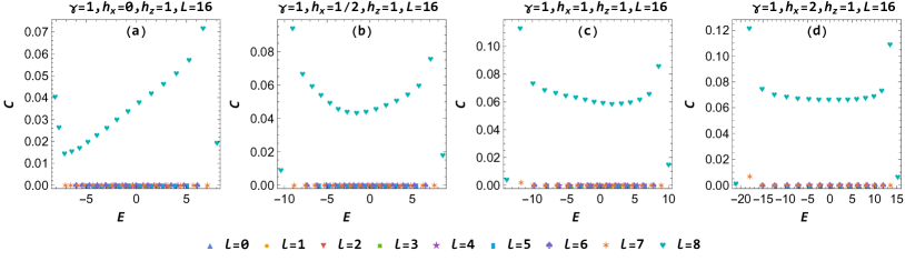
Figure 1: The concurrence between two qubits in the LMG model calculated using the bootstrap method. We use different colored symbols to represent states with different angular quantum number $l$.

5 Tangle and residual tangle

When an entire system is in a pure state, one can quantify the entanglement between a single qubit and the remainder of the system using the entanglement entropy, i.e., the von Neumann entropy of the one-qubit density matrix $\rho$ given by

$$S=-\textrm{tr}(\rho\log\rho).$$ (5.1)

Alternatively, one may use the tangle

$$\tau=4\det\rho.$$ (5.2)

The entanglement entropy and tangle are equivalent and they are simply related as

$$S=-\frac{1+\sqrt{1-\tau}}{2}\log\frac{1+\sqrt{1-\tau}}{2}-\frac{1-\sqrt{1-\tau}}{2}\log\frac{1-\sqrt{1-\tau}}{2}.$$ (5.3)

The tangle between two qubits is $\tau=C^{2}$ with $C$ being the concurrence, which applies even when the two qubits are in a mixed state. The monogamy of the entanglement is encoded in the Coffman-Kundu-Wootters (CKW) inequality [33, 34]

$$\sum_{j=2}^{L}C_{1j}^{2}\leq\tau_{1(23\cdots L)},$$ (5.4)

where $C_{1j}$ is the concurrence between the first qubit and the $j$-th qubit and $\tau_{1(23\cdots L)}$ is the tangle between the first qubit and the rest qubits. From the CKW inequality one may define the residual tangle as [33]

$$\Delta\tau_{1(23\cdots L)}=\tau_{1(23\cdots L)}-\sum_{j=2}^{L}C_{1j}^{2},$$ (5.5)

which measures part of the multipartite entanglement that is not encoded in double-qubit entanglement.

In LMG model, we consider the energy eigenstates that are invariant under the exchange of two arbitrary qubits. In such an eigenstate, the single-qubit density matrix is written as

$$\rho=\sum_{\alpha=0}^{3}f_{\alpha}\sigma^{\alpha},$$ (5.6)

with

$$f_{0}=\frac{1}{2},~{}~{}f_{1}=\frac{1}{L}\langle J_{x}\rangle,~{}~{}f_{2}=\frac{1}{L}\langle J_{y}\rangle,~{}~{}f_{3}=\frac{1}{L}\langle J_{z}\rangle.$$ (5.7)

The tangle between one qubit and the rest qubits is

$$\tau=1-\frac{4}{L^{2}}(\langle J_{x}\rangle^{2}+\langle J_{y}\rangle^{2}+\langle J_{z}\rangle^{2}).$$ (5.8)

The CKW inequality becomes

$$(L-1)C^{2}\leq\tau,$$ (5.9)

with $C$ being the concurrence between two qubits. The residual tangle is

$$\Delta\tau=\tau-(L-1)C^{2}.$$ (5.10)

The tangle and residual tangle are obtained from the bootstrap analysis, as shown in figure 2. The tangle is approximately a function of the energy $E$ and independent of the quantum number $l$. The residual tangle is almost the same as the tangle, except that the residual tangle in states with quantum number $l=\frac{L}{2}$ is slightly smaller than the tangle. States in the middle of the spectrum tend to have larger tangles and residual tangles, while states near the ground state and the highest-energy state have smaller tangles and residual tangles. This indicates that states in the middle of the spectrum have stronger entanglement and that most of the entanglement therein is stored as multipartite entanglement.

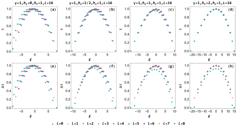
Figure 2: The tangle (top panels) and residual tangle (bottom panels) between a single qubit and the rest qubits in the LMG model obtained from the bootstrap analysis. We use different colored symbols to represent states with different angular quantum number $l$.

6 Quantum Fisher information

From the bootstrap analysis, we can also calculate the quantum Fisher information (QFI), which can be used as an entanglement witness to characterize multipartite entanglement as shown in [26, 27, 28].

In a pure state, for the operators $J_{x,y,z}$ there is the QFI

$$F_{x,y,z}=4(\langle J_{x,y,z}^{2}\rangle-\langle J_{x,y,z}\rangle^{2}).$$ (6.1)

For a general direction

$$n=(\sin\theta\cos\phi,\sin\theta\sin\phi,\cos\theta),$$ (6.2)

there is the operator $J_{n}=n_{x}J_{x}+n_{y}J_{y}+n_{y}J_{y}$, and corresponding QFI is

$$F_{n}=4(\langle J_{n}^{2}\rangle-\langle J_{n}\rangle^{2}).$$ (6.3)

For a state one may define the QFI related quantites

$$F_{\rm max}\equiv\max_{\theta,\phi}F_{n},$$ (6.4)

and

$$F_{\rm sum}\equiv\sum_{i=x,y,z}F_{i}.$$ (6.5)

A pure state of $m$ particles is called separable if it could written as the direct product of $m$ one-particle states. For all separable pure states, there are [26]

$$F_{\rm max}\leq L$$ (6.6)

and [28]

$$F_{\rm sum}\leq 2L.$$ (6.7)

If for a pure state there is

$$F_{\rm max}>L,$$ (6.8)

or

$$F_{\rm sum}>2L,$$ (6.9)

there exists entanglement in the state. In other words, we have

$$({\rm not~{}entangled})\Leftrightarrow{\rm separable}\Rightarrow(F_{\rm max}\leq L{\rm~{}and~{}}F_{\rm sum}\leq 2L),$$ (6.10)

or equivalently

$${\rm entangled}\Leftrightarrow({\rm not~{}separable})\Leftarrow(F_{\rm max}>L{\rm~{}or~{}}F_{\rm sum}>2L).$$ (6.11)

If $F_{\rm max}\leq L$ and $F_{\rm sum}\leq 2L$, it does not necessarily mean there is no entanglement. The constraints (6.8) and (6.9) are just sufficient but not necessary conditions for the existence of entanglement.

A pure state is called $k$-producible if it can be written as the direct product of several pure states, with each pure state involving at most $k$ particles. It is easy to see from the definition that a $k$-producible state is automatically $(k+1)$-producible. The special case of a 1-producible state is simply a separable state. A $k$-producible state that is not $(k-1)$-producible is genuinely $k$-partite entangled. For general $k$-producible states, there are upper bounds [28]

$$F_{\rm max}\leq F_{\rm max}^{k},$$ (6.12)

$$F_{\rm sum}\leq F_{\rm sum}^{k},$$ (6.13)

with the definitions

$$F_{\rm max}^{k}\equiv nk^{2}+(L-nk)^{2},$$ (6.14)

$$F_{\rm sum}^{k}\equiv\left\{\begin{array}[]{ll}nk(k+2)+(L-nk)(L-nk+2)&{\rm if~{}}L-nk\neq 1\\ nk(k+2)+2&{\rm if~{}}L-nk=1\end{array}\right.\!\!\!\!,$$ (6.15)

and $n$ being the integer part of $\frac{L}{k}$. When $k=1$, the state is just separable, and we have $F_{\rm max}^{1}=L$, which is the same as the bound (6.6), and $F_{\rm sum}^{1}=3L$, which is looser than the bound (6.7). In the following we will redefine for the $k=1$ case $F_{\rm sum}^{1}\equiv 2L$. In other words, we have

$$F_{\rm sum}^{k}\equiv\left\{\begin{array}[]{lll}2L&{\rm if~{}}k=1\\ nk(k+2)+(L-nk)(L-nk+2)&{\rm if~{}}k>1{\rm~{}and~{}}L-nk\neq 1\\ nk(k+2)+2&{\rm if~{}}k>1{\rm~{}and~{}}L-nk=1\end{array}\right.\!\!\!\!.$$ (6.16)

Note that a $k$-producible state is automatically a $(k+1)$-producible state, and there are always $F_{\rm max}^{k}\leq F_{\rm max}^{k+1}$ and $F_{\rm sum}^{k}\leq F_{\rm sum}^{k+1}$ as required.

When for a state there is

$$F_{\rm max}>F_{\rm max}^{k},$$ (6.17)

or

$$F_{\rm sum}>F_{\rm sum}^{k},$$ (6.18)

the state has at least genuine multipartite entanglement of $k+1$ particle, or, in other words, the entanglement depth of the state is larger than $k$. Especially, when

$$F_{\rm max}>F_{\rm max}^{L-1}=(L-1)^{2}+1,$$ (6.19)

or

$$F_{\rm sum}>F_{\rm sum}^{L-1}=L^{2}+1,$$ (6.20)

the entanglement depth of the state takes the largest value $L$, and any tripartite subsystems in the system is genuinely multipartite entangled.

From the bootstrap analysis, we obtain the energy spectrum and the corresponding expectation values, as well as the quantum Fisher information (QFI). We show the results for various parameters in figure 3. For small $l$, the bounds (6.14) and (6.16) give approximately the same results, while for large $l$, the bound (6.16) is more effective than (6.14). We observe that states in the middle of the spectrum and with larger quantum number $l$ tend to have stronger multipartite entanglement. For every energy window, the multipartite entanglement increases with $l$.

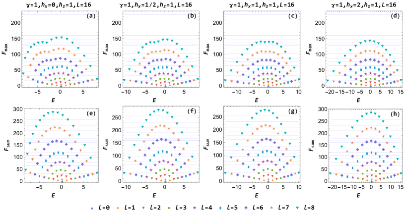
Figure 3: Quantum Fisher information (QFI) in the spectrum of the LGM model from bootstrap. We use different colored symbols to represent states with different angular quantum number $l$. The thin blue lines are the bounds (6.14) and (6.16), with $k$ taking values in the range $[1,L-1]$ from the bottom to the top.

7 Conclusion and discussions

In this study, we have elaborated on a methodology for determining the entanglement attributes of eigenstates for particular Hamiltonians, all without having to directly compute the eigenstates. The core approach employs consistency relations, as given by Eqs. (2.8) and (2.9), augmented with additional constraints as in Eqs. (2.14) and (2.15). Utilizing these, we can derive the operator expectation values for all eigenstates. From these expectation values, entanglement measures such as concurrence between two qubits, tangle, residual tangle, and quantum Fisher information can be explicitly calculated for all eigenstates simultaneously. Perhaps unsurprisingly, our findings reveal that eigenstates in the central part of the spectrum for the LMG model exhibit significant multipartite entanglement but limited concurrence. This observation aligns well with the expected behavior based on the monogamy property of entanglement. We have corroborated this through calculations involving both residual tangle and quantum Fisher information.

While the current paper is focused on the Lipkin-Meshkov-Glick (LMG) model, which includes both transverse and longitudinal external magnetic fields, the methodology is extendable to Hamiltonians of the form given in Eq. (2.4) without any major modifications.

It’s worth noting that the computational complexity of our bootstrap method increases exponentially with the size of the system. However, this shouldn’t be viewed as a limitation since it allows us to obtain all correlation functions for all eigenstates in a unified manner. One potential avenue for future research could be identifying an effective truncation scheme that enables the extraction of ground-state or low-energy-state properties with polynomial computational effort. The specific nature of such a truncation remains an open question at this stage.

Additionally, due to the Hamiltonian’s permutation property as expressed in Eq. (2.4), we did not need to employ the positivity condition shown in Eq. (2.10). For short-range Hamiltonians, such as the transverse field Ising chain with or without longitudinal magnetic fields, additional operators would need to be incorporated into the bootstrap framework to calculate entanglement measures like the concurrence of two qubits. Efficient strategies for identifying the necessary operators for these kinds of models require further investigation.

Appendix A Bootstrapping a toy model

We consider the simple toy model with Hamiltonian

$$H=\frac{1}{2}\sum_{j=1}^{L}\sigma_{z}^{j}.$$ (A.1)

We define $J_{z}\equiv\frac{1}{2}\sum_{j=1}^{L}\sigma_{z}^{j}$ and choose the set $\mathcal{S}$ generated by the operators

$$\{J_{z}^{\alpha},\alpha=0,1,2,\cdots,L\}.$$ (A.2)

We only consider the cases with even integer $L$, and it is similar for cases with odd integer $L$. From the Cayley-Hamilton theorem

$$J_{z}\prod_{m=1}^{L/2}(J_{z}^{2}-m^{2})=0,$$ (A.3)

one may write higher order powers of $J_{z}$ in terms of operators in $\mathcal{S}$. For example, there are

$$L=2:~{}J_{z}^{3}=J_{z},$$

$$L=4:~{}J_{z}^{5}=5J_{z}^{3}-4J_{z}.$$ (A.4)

Note that $J_{z}^{0}=I$ is just the identity operator that so there is $v_{0}=1$. From the constraint (2.8) with $\alpha=0,1,\cdots,L-1$, we get

$$v_{\alpha+1}=Ev_{\alpha},~{}\alpha=0,1,\cdots,L-1,$$ (A.5)

and so we have

$$v_{\alpha}=E^{\alpha},\alpha=0,1,\cdots,L.$$ (A.6)

From the constraint (2.8) with $\alpha=L$, we further obtain

$$E\sum_{m=0}^{L/2}(E^{2}-m^{2})=0.$$ (A.7)

Finally we get $L+1$ different solutions of the energy and expectation values

$$E=m,~{}v_{\alpha}=m^{\alpha},~{}\alpha=0,1,\cdots,L-1,~{}m=0,\pm 1,\cdots,\pm\frac{L}{2},$$ (A.8)

which are just the exact solutions. Note that to obtain the above solutions we have not used the constraint (2.9) which is automatically satisfied by the solutions to the constraints (2.8).

Needless to say, in this appendix, we have used a difficult method to solve a simple problem.

Appendix B Solving LMG model from algebra of angular momentum

The spectrum of the LMG model can be solved exactly using the algebra of angular momentum, as originally proposed by Lipkin in [18]. This approach involves writing the Hamiltonian in a different basis, which results in a significantly simpler form.

At each site, there exists the fundamental representation $\bf 2$, i.e. the spin-1/2 representation, of the SU(2) group. For the entire system, the representation of the SU(2) group is reducible and can be expressed as

$${\bf 2}^{\otimes L}=\bigoplus_{l=l_{\rm min}}^{L/2}({\bf 2\textit{{l}}+1})_{d_{j}},$$ (B.1)

where the duplicate number of the $({\bf 2\textit{{l}}+1})$ representation, i.e. the spin-$l$ representation, is given by

$$d_{l}=\frac{2l+1}{L+1}C_{L+1}^{\frac{L}{2}+l+1}.$$ (B.2)

There are $l_{\rm min}=0$ for an even integer $L$, and $l_{\rm min}=\frac{1}{2}$ for an odd integer $L$. For the special case where $l=L/2$, the duplicate number $d_{L/2}=1$.

Noting the Hamiltonian (3.3), for $l=0,\frac{1}{2},1,\frac{3}{2},\cdots$ we define the operator

$$H^{(l)}=-\frac{1}{L}\Big{[}\frac{1+\gamma}{2}(J_{x}^{(l)})^{2}+\frac{1-\gamma}{2}(J_{y}^{(l)})^{2}\Big{]}+\frac{1}{4}I_{2l+1}-h_{x}J_{x}^{(l)}-h_{z}J_{z}^{(l)},$$ (B.3)

with $J_{x}^{(l)}$, $J_{y}^{(l)}$, $J_{z}^{(l)}$ being the components of the spin-$l$ angular momentum and $I_{2l+1}$ being the $(2l+1)\times(2l+1)$ identity matrix. Then from representation reduction, the Hamiltonian (3.1) is similar to

$$H\sim\bigoplus_{l=l_{\rm min}}^{L/2}H^{(l)}_{d_{l}}.$$ (B.4)

We have used the same symbol $d_{l}$ (B.2) as the duplicate number of each block $H^{(l)}$. For the Hamiltonian $H$, every eigenvalue of $H^{(l)}$ has degeneracy $d_{l}$.

As shown in (B.4), the Hamiltonian can be decomposed into direct product of several blocks in a specific basis, and the explicit transformation relation between the block-diagonal basis and the $\sigma_{z}$ basis is not of concern to us. In each block, one may obtain the eigenvalues and eigenstates of the Hamiltonian and compute the expectation values of operators that can be expressed in terms of $J_{x},J_{y},J_{z}$ given in (3.2). For the sector $l=L/2$, the energy eigenstates are superpositions of the $L$ states.

$$|L/2,m\rangle=\frac{1}{\sqrt{C_{L/2}^{m}}}\sum_{1\leq j_{1}<j_{2}<\cdots<j_{m}\leq L}|\uparrow_{j_{1}}\uparrow_{j_{2}}\cdots\uparrow_{j_{m}}\rangle,~{}m=\frac{L}{2},\frac{L}{2}-1,\cdots,-\frac{L}{2}.$$ (B.5)

Here, $|\uparrow_{j_{1}}\uparrow_{j_{2}}\cdots\uparrow_{j_{m}}\rangle$ denotes the state in which the $m$ sites $j_{1},j_{2},\cdots,j_{m}$ have up spins and all other sites have down spins. All the states (B.5) are invariant under an arbitrary permutation of the sites, and so all the eigenstates in the sector $l=L/2$ are also permutation invariant. Generally, the eigenstates in the other sectors are not permutation invariant.

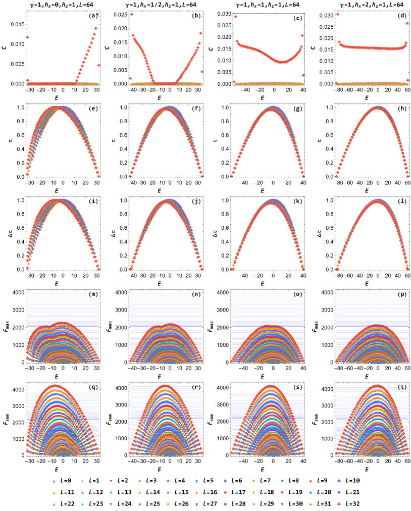
Figure 4: The concurrence between two sites (first row), tangle (second row) and residual tangle (third row) between one site and the other sites, as well as quantum Fisher information (last two rows) of the entire spectrum in the LMG model derived from the algebra of angular momentum. We utilize distinctly colored symbols to distinguish states with distinct quantum numbers $l$.

Figure 5: The concurrences between two sites $C_{12}$ (first row), the tangle (second row) and the residual tangle (last row) between one site with other sites in the entire spectrum of the LMG model derived from block diagonalization. We utilize distinctly colored symbols to distinguish states with distinct quantum numbers $l$.

Similar to the calculations of sections 4, 5, 6, we utilize the expectation values of $\langle J_{\alpha}\rangle$ and $\langle J_{\alpha}J_{\beta}\rangle$ with $\alpha,\beta=x,y,z$ to compute the concurrence between two arbitrary sites, the tangle and residual tangle between one site and the other sites, and the quantum Fisher information. The permutation invariance is necessary for the calculations of the concurrence and residual tangle, and they are only calculated for the eigenstates in the $l=\frac{L}{2}$ sector. To calculate the tangle and quantum Fisher information, only translation invariance is required, and then we can compute them for all the eigenstates. For small $L$, such as $L\leq 16$, our results align with the ones obtained through bootstrap. Furthermore, we are able to obtain results for significantly larger $L$ values, as demonstrated in Figure 4. The results for the larger $L$ values exhibit a qualitatively similar trend to the results obtained for smaller $L$ values via bootstrap.

Appendix C Solving LMG model from block diagonalization

The LMG model with the Hamiltonian can also be solved through exact block diagonalization, as described in [35]. The Hamiltonian (3.1) exhibits translational invariance, and the momentum is a conserved quantity. In the sector possessing a fixed momentum $k$, we are able to find the simultaneous eigenstates of the Hamiltonian and the angular momentum $J^{2}=J_{x}^{2}+J_{y}^{2}+J_{y}^{2}$. By construction, every state displays translational invariance, although it may not necessarily be permutation invariant. However, all the states with angular quantum number $l=L/2$ are permutation invariant. For states with $l<L/2$, there exists a degeneracy among states with fixed $E$, $k$, and $l$, resulting in ambiguous wavefunctions for these states.

For each state, we compute the concurrences $C_{j_{1}j_{2}}$ with $(j_{1},j_{2})=(1,2),(1,1+\lfloor{L}/{4}\rfloor),(1,1+\lfloor{L}/{2}\rfloor)$ as well as the tangle and residual tangle between one site and other sites. In Figure 5, we present examples of the results for $L=16$. For states with $l=L/2$, the outcomes align with those attained from bootstrap and angular momentum algebra. However, for other states, disparities may arise from the arbitrary definition of the states, leading to differences from the results obtained through bootstrap and angular momentum algebra.

References

- [1] D. Poland, S. Rychkov and A. Vichi, The Conformal Bootstrap: Theory, Numerical Techniques, and Applications, Rev. Mod. Phys. 91, 015002 (2019), [arXiv:1805.04405].
- [2] D. Simmons-Duffin, The Conformal Bootstrap, in TASI 2015: New Frontiers in Fields and Strings, pp. 1–74, 2017. arXiv:1602.07982. DOI.
- [3] X. Han, S. A. Hartnoll and J. Kruthoff, Bootstrapping Matrix Quantum Mechanics, Phys. Rev. Lett. 125, 041601 (2020), [arXiv:2004.10212].
- [4] D. Berenstein and G. Hulsey, Bootstrapping Simple QM Systems, arXiv:2108.08757.
- [5] J. Bhattacharya, D. Das, S. K. Das, A. K. Jha and M. Kundu, Numerical bootstrap in quantum mechanics, Phys. Lett. B 823, 136785 (2021), [arXiv:2108.11416].
- [6] Y. Aikawa, T. Morita and K. Yoshimura, Application of bootstrap to a term, Phys. Rev. D 105, 085017 (2022), [arXiv:2109.02701].
- [7] D. Berenstein and G. Hulsey, Bootstrapping more QM systems, J. Phys. A 55, 275304 (2022), [arXiv:2109.06251].
- [8] S. Tchoumakov and S. Florens, Bootstrapping Bloch bands, J. Phys. A 55, 015203 (2022), [arXiv:2109.06600].
- [9] B.-n. Du, M.-x. Huang and P.-x. Zeng, Bootstrapping Calabi–Yau quantum mechanics, Commun. Theor. Phys. 74, 095801 (2022), [arXiv:2111.08442].
- [10] D. Berenstein and G. Hulsey, Semidefinite programming algorithm for the quantum mechanical bootstrap, Phys. Rev. E 107, L053301 (2023), [arXiv:2209.14332].
- [11] C. O. Nancarrow and Y. Xin, Bootstrapping the gap in quantum spin systems, arXiv:2211.03819.
- [12] L. Amico, R. Fazio, A. Osterloh and V. Vedral, Entanglement in many-body systems, Rev. Mod. Phys. 80, 517 (2008), [arXiv:quant-ph/0703044].
- [13] M. B. Hastings, I. González, A. B. Kallin and R. G. Melko, Measuring Renyi Entanglement Entropy in Quantum Monte Carlo Simulations, Phys. Rev. Lett. 104, 157201 (2010), [arXiv:1001.2335].
- [14] D. A. Abanin and E. Demler, Measuring Entanglement Entropy of a Generic Many-Body System with a Quantum Switch, Phys. Rev. Lett. 109, 020504 (2012), [arXiv:1204.2819].
- [15] A. Daley, H. Pichler, J. Schachenmayer and P. Zoller, Measuring entanglement growth in quench dynamics of bosons in an optical lattice, Phys. Rev. Lett. 109, 020505 (2012), [arXiv:1205.1521].
- [16] R. Islam, R. Ma, P. M. Preiss, M. E. Tai, A. Lukin, M. Rispoli and M. Greiner, Measuring entanglement entropy in a quantum many-body system, Nature 528, 77 (2015), [arXiv:1509.01160].
- [17] P. Calabrese and J. Cardy, Entanglement entropy and conformal field theory, J. Phys. A: Math. Gen. 42, 504005 (2009), [arXiv:0905.4013].
- [18] H. J. Lipkin, N. Meshkov and A. J. Glick, Validity of many-body approximation methods for a solvable model: (I). Exact solutions and perturbation theory, Nucl. Phys. 62, 188–198 (1965).
- [19] N. Meshkov, A. J. Glick and H. J. Lipkin, Validity of many-body approximation methods for a solvable model: (II). Linearization procedures, Nucl. Phys. 62, 199–210 (1965).
- [20] A. Glick, H. Lipkin and N. Meshkov, Validity of many-body approximation methods for a solvable model: (III). Diagram summations, Nucl. Phys. 62, 211–224 (1965).
- [21] J. Vidal, R. Mosseri and J. Dukelsky, Entanglement in a first-order quantum phase transition, Phys. Rev. A 69, 054101 (2004), [arXiv:cond-mat/0312130].
- [22] J. Vidal, G. Palacios and R. Mosseri, Entanglement in a second-order quantum phase transition, Phys. Rev. A 69, 022107 (2004), [arXiv:cond-mat/0305573].
- [23] S. Dusuel and J. Vidal, Finite-size scaling exponents of the Lipkin-Meshkov-Glick model, Phys. Rev. Lett. 93, 237204 (2004), [arXiv:cond-mat/0408624].
- [24] J. Ma and X. Wang, Fisher information and spin squeezing in the Lipkin-Meshkov-Glick model, Phys. Rev. A 80, 012318 (2009), [arXiv:0905.0245].
- [25] G. Salvatori, A. Mandarino and M. G. A. Paris, Quantum metrology in Lipkin-Meshkov-Glick critical systems, Phys. Rev. A 90, 022111 (2014), [arXiv:1406.5766].
- [26] L. Pezze and A. Smerzi, Entanglement, Nonlinear Dynamics, and the Heisenberg Limit, Phys. Rev. Lett. 102, 100401 (2009), [arXiv:0711.4840].
- [27] P. Hyllus, W. Laskowski, R. Krischek, C. Schwemmer, W. Wieczorek, H. Weinfurter, L. Pezzé and A. Smerzi, Fisher information and multiparticle entanglement, Phys. Rev. A 85, 022321 (2012), [arXiv:1006.4366].
- [28] G. Tóth, Multipartite entanglement and high-precision metrology, Phys. Lett. A 85, 022322 (2012), [arXiv:1006.4368].
- [29] P. Hauke, M. Heyl, L. Tagliacozzo and P. Zoller, Measuring multipartite entanglement through dynamic susceptibilities, Nat. Phys. 12, 778–782 (2016), [arXiv:1509.01739].
- [30] W. K. Wootters, Entanglement of formation of an arbitrary state of two qubits, Phys. Rev. Lett. 80, 2245–2248 (1998), [arXiv:quant-ph/9709029].
- [31] L. Amico, A. Osterloh, F. Plastina, R. Fazio and G. Massimo Palma, Dynamics of entanglement in one-dimensional spin systems, Phys. Rev. A 69, 022304 (2004), [arXiv:quant-ph/0307048].
- [32] A. Fubini, T. Roscilde, V. Tognetti, M. Tusa and P. Verrucchi, Reading entanglement in terms of spin configurations in quantum magnets, Eur. Phys. J. D 38, 563–570 (2006), [arXiv:cond-mat/0505280].
- [33] V. Coffman, J. Kundu and W. K. Wootters, Distributed entanglement, Phys. Rev. A 61, 052306 (2000), [arXiv:quant-ph/9907047].
- [34] T. J. Osborne and F. Verstraete, General Monogamy Inequality for Bipartite Qubit Entanglement, Phys. Rev. Lett. 96, 220503 (2006), [arXiv:quant-ph/0502176].
- [35] A. W. Sandvik, Computational Studies of Quantum Spin Systems, AIP Conf. Proc. 1297, 135 (2010), [arXiv:1101.3281].