Noise-induced stochastic Nash equilibrium

Abstract

In order to better understand the impact of environmental stochastic fluctuations on the evolution of animal behavior, we introduce the concept of a stochastic Nash equilibrium (SNE) that extends the classical concept of a Nash equilibrium (NE). Based on a stochastic stability analysis of a linear evolutionary game with temporally varying payoffs, we address the question of the existence of a SNE, either weak when the geometric mean payoff against it is the same for all other strategies or strong when it is strictly smaller for all other strategies, and its relationship with a stochastically evolutionarily stable (SES) strategy. While a strong SNE is always SES, this is not necessarily the case for a weak SNE. We give conditions for a completely mixed weak SNE not to be SES and to coexist with at least two strong SNE. More importantly, we show that a pair of two completely mixed strong SNE can emerge as the noise level increases. This not only indicates that a noise-induced SNE may possess some properties that a NE cannot possess, such as being completely mixed and strong, but also illustrates the complexity of evolutionary game dynamics in a stochastic environment.

Introduction. As it is well known, a Nash equilibrium (NE) is the core concept of non-cooperative games [1], and it has had a profound impact on economics, biology and social sciences [3, 5, 6, 2, 4]. For linear evolutionary games based on payoff matrices [7, 4], the equilibrium condition for an evolutionarily stable strategy (ESS) is exactly the definition of a NE, which is a strategy that is the best reply to itself [2, 7]. It is also known in this framework that, while an ESS must be a NE, the inverse is not necessarily true. This is the case, however, for a strict NE, which is strictly better against itself than any other strategy [2, 7]. Moreover, if a completely mixed strategy is a NE, then it must be unique and it can never be a strict NE. In particular, this implies that it is impossible to have two or more completely mixed strategies that are both ESS [7].

Recently, in order to explore the impact of environmental stochastic fluctuations on evolutionary game dynamics, Zheng et al. [8, 9] (see also Feng et al. [10, 11]) developed the concept of stochastic evolutionary stability based on conditions for stochastic stability of equilibria in stochastic recurrence equations (or stochastic replicator dynamics). A stochastically evolutionarily stable (SES) strategy is defined as a strategy such that, if all the members of the population adopt it, then the probability for at least any slightly perturbed strategy to successfully invade the population under the influence of natural selection is arbitrarily low.

Then, a challenging question naturally arises: how should we define a stochastic Nash equilibrium (SNE) in the case of random payoffs that would extend the concept of a NE in the case of deterministic payoffs, and what would be the relationships between a SNE and a SES strategy in stochastic evolutionary games. Analogously to the classic definition of a NE [3, 7, 12, 4], a SNE should be defined as a strategy that is the best reply to itself but taking into account the uncertainty in the payoffs in a stochastic environment. Hence, a SNE should not only be regarded as an extension of a NE, but also as a concept to capture the effect of environmental noise on the equilibrium structure in evolutionary game dynamics.

In this letter, from a stochastic stability analysis of the discrete-time dynamics of a linear evolutionary game with a random payoff matrix, we define the concepts of weak SNE and strong SNE, and we examine conditions for their existence and co-existence. Our goal is not only to show how stochastic environmental noise can induce the emergence of a SNE, called a noise-induced SNE, which does not have any equivalent in a constant environment, but also to provide a theoretical framework for studying the role of environment noise in shaping complex equilibrium structures and evolutionary patterns in game dynamics.

Stochastic Nash equilibrium. We consider an evolutionary game in an infinite population with discrete, non-overlapping generations. There are two pure strategies in use, denoted by $S_{1}$ and $S_{2}$, and the payoffs received following pairwise interactions at time step $t\geq 1$ are given by the entries of the game matrix

$$\mathbf{A}(t) =\begin{pmatrix}a_{11}(t)&a_{12}(t)\\ a_{21}(t)&a_{22}(t)\end{pmatrix},$$ (1)

where $a_{ij}(t)$ denotes the payoff to strategy $S_{i}$ against strategy $S_{j}$ at time step $t\geq 1$ for $i,j=1,2$. For simplicity, these payoffs are assumed to be positive random variables that are uniformly bounded below and above by some positive constants. Therefore, there exist real numbers $A$ and $B$ such that $0<A\leq a_{ij}(t)\leq B$ for $i,j=1,2$ and all $t\geq 1$ [8]. Moreover, the probability distribution of $a_{ij}(t)$ for $i,j=1,2$ do not depend on $t\geq 1$. The means, variances, and covariances of these random payoffs are given by $\left<a_{ij}(t)\right>=\bar{a}_{ij}$, $\left<\big{(}a_{ij}(t)-\bar{a}_{ij}\big{)}^{2}\right>=\sigma_{ij}^{2}$ and $\left<\big{(}a_{ij}(t)-\bar{a}_{ij}\big{)}\big{(}a_{kl}(t)-\bar{a}_{kl}\big{)}\right>=\sigma_{ij,kl}$, respectively, for $i,j,k,l=1,2$ with $(i,j)\neq(k,l)$. As for $s\neq t$, the payoffs $a_{ij}(s)$ and $a_{kl}(t)$ are assumed to be independent so that $\left<\big{(}a_{ij}(s)-\bar{a}_{ij}\big{)}\big{(}a_{kl}(t)-\bar{a}_{kl}\big{)}\right>=0$ for $i,j,k,l=1,2$.

Consider a population consisting of individuals using only two mixed strategies $\mathbf{x}=(x,1-x)$ and $\hat{\mathbf{x}}=(\hat{x},1-\hat{x})$ with $x,\hat{x}\in[0,1]$. The payoff matrix for these two mixed strategies at time step $t\geq 1$ is given by

$$\begin{pmatrix}\mathbf{x}\cdot\mathbf{A}(t)\mathbf{x}&\mathbf{x}\cdot\mathbf{A}(t)\hat{\mathbf{x}}\\ \hat{\mathbf{x}}\cdot\mathbf{A}(t)\mathbf{x}&\hat{\mathbf{x}}\cdot\mathbf{A}(t)\hat{\mathbf{x}}\end{pmatrix},$$ (2)

where $\mathbf{x}\cdot\mathbf{A}(t)\mathbf{x}$ (or $\mathbf{x}\cdot\mathbf{A}(t)\hat{\mathbf{x}}$) is the payoff to strategy $\mathbf{x}$ against strategy $\mathbf{x}$ (or strategy $\hat{\mathbf{x}}$), and $\hat{\mathbf{x}}\cdot\mathbf{A}(t)\mathbf{x}$ (or $\hat{\mathbf{x}}\cdot\mathbf{A}(t)\hat{\mathbf{x}}$) is the payoff to strategy $\hat{\mathbf{x}}$ against strategy $\mathbf{x}$ (or strategy $\hat{\mathbf{x}}$) [8].

Let $q(t)$ be the frequency of strategy $\mathbf{x}$ at time step $t\geq 1$. Assuming random pairwise interactions, the average payoffs to strategies $\mathbf{x}$ and $\hat{\mathbf{x}}$ at time step $t\geq 1$ are given by $\pi_{\mathbf{x}}(t)=q(t)\mathbf{x}\cdot\mathbf{A}(t)\mathbf{x}+(1-q(t))\mathbf{x}\cdot\mathbf{A}(t)\hat{\mathbf{x}}$ and $\pi_{\hat{\mathbf{x}}}(t)=q(t)\hat{\mathbf{x}}\cdot\mathbf{A}(t)\mathbf{x}+(1-q(t))\hat{\mathbf{x}}\cdot\mathbf{A}(t)\hat{\mathbf{x}}$, respectively. Taking the average payoff as fitness, the frequency of strategy $\mathbf{x}$ at time step $t+1$ can be expressed as

$$q(t+1) =\frac{q(t)\pi_{\mathbf{x}}(t)}{q(t)\pi_{\mathbf{x}}(t)+(1-q(t))\pi_{\hat{\mathbf{x}}}(t)},$$ (3)

which is a stochastic recurrence equation [8].

By definition, the strategy $\hat{\mathbf{x}}$ is stochastically evolutionarily stable (SES) if the boundary equilibrium $q(t)=0$ is stochastically locally stable (SLS) for all possible $\mathbf{x}\neq\hat{\mathbf{x}}$ [8]. It can be shown that $\hat{\mathbf{x}}$ is SES if and only if

$$\left<\log\mathbf{x}\cdot\mathbf{A}(t)\hat{\mathbf{x}}\right>\leq\left<\log\hat{\mathbf{x}}\cdot\mathbf{A}(t)\hat{\mathbf{x}}\right>$$ (4)

for all possible $\mathbf{x}$, and

$$\left<\frac{\hat{\mathbf{x}}\cdot\mathbf{A}(t)\mathbf{x}}{\hat{\mathbf{x}}\cdot\mathbf{A}(t)\hat{\mathbf{x}}}\right>-\left<\frac{\mathbf{x}\cdot\mathbf{A}(t)\mathbf{x}}{\hat{\mathbf{x}}\cdot\mathbf{A}(t)\hat{\mathbf{x}}}\right>=-(\hat{x}-x)^{2}D>0$$ (5)

with

$$D =\left<\frac{\big{(}a_{11}(t)-a_{12}(t)-a_{21}(t)+a_{22}(t)\big{)}^{2}}{a_{11}(t)a_{22}(t)-a_{12}(t)a_{21}(t)}\right>$$ (6)

in the case of an equality in Eq. (4) for all possible $\mathbf{x}$ (see [8] and the Appendix for the expression of $D$).

By analogy with the conditions for equilibrium and stability of an evolutionarily stable strategy (ESS) (see p. 63 in [7]), the first condition above is used to define a stochastic Nash equilibrium (SNE). This corresponds to a strategy that is the best reply to itself in a stochastic environment based on the geometric means of the payoffs rather than their arithmetic means.

Let us recall that the geometric mean of a random variable $X$ is defined as $GM\left<X\right>=\exp(\left<\log X\right>)$. Therefore, Eq. (4) is equivalent to

$$GM\left<\mathbf{x}\cdot\mathbf{A}(t)\hat{\mathbf{x}}\right>\leq GM\left<\hat{\mathbf{x}}\cdot\mathbf{A}(t)\hat{\mathbf{x}}\right>$$ (7)

for all possible $\mathbf{x}\neq\hat{\mathbf{x}}$. This is the condition for $\hat{\mathbf{x}}$ to be a SNE. In the special case where $GM\left<\mathbf{x}\cdot\mathbf{A}(t)\hat{\mathbf{x}}\right>=GM\left<\hat{\mathbf{x}}\cdot\mathbf{A}(t)\hat{\mathbf{x}}\right>$ for all $\mathbf{x}\neq\hat{\mathbf{x}}$, the strategy $\hat{\mathbf{x}}$ will be called a weak stochastic Nash equilibrium (weak SNE). At the other extreme, if $GM\left<\mathbf{x}\cdot\mathbf{A}(t)\hat{\mathbf{x}}\right><GM\left<\hat{\mathbf{x}}\cdot\mathbf{A}(t)\hat{\mathbf{x}}\right>$ for all $\mathbf{x}\neq\hat{\mathbf{x}}$, then $\hat{\mathbf{x}}$ will be said a strong stochastic Nash equilibrium (strong SNE). Note that the SNE condition is necessary but not sufficient for stochastic evolutionary stability (SES), while the condition for a strong SNE is sufficient but not necessary. In other words, we have the following implications:

$$\textrm{ strong SNE }\Rightarrow\textrm{ SES }\Rightarrow\textrm{ SNE }$$

Equilibrium structure. In this section, we examine the equilibrium structure of the system. In order to distinguish the pure strategies $S_{1}$ and $S_{2}$, we assume throughout that $\mathbf{P}\left(a_{11}(t)=a_{21}(t),a_{22}(t)=a_{12}(t)\right)<1$, which is equivalent to saying that $S_{1}$ and $S_{2}$ have different payoffs with positive probability. As shown in the Appendix, a strategy $\mathbf{x^{*}}=(x^{*},1-x^{*})$ such that $\mathbf{P}\left(\big{(}\mathbf{A}(t)\mathbf{x^{*}}\big{)}_{1}=\big{(}\mathbf{A}(t)\mathbf{x^{*}}\big{)}_{2}\right)<1$ is a strong SNE if and only if

$$\left<\frac{\big{(}\mathbf{A}(t)\mathbf{x^{*}}\big{)}_{1}-\big{(}\mathbf{A}(t)\mathbf{x^{*}}\big{)}_{2}}{\mathbf{x^{*}}\cdot\mathbf{A}(t)\mathbf{x^{*}}}\right>\begin{cases}\leq 0&\textrm{ if }x^{*}=0,\\ \geq 0&\textrm{ if }x^{*}=1,\\ =0&\textrm{ if }0<x^{*}<1,\end{cases}$$ (8)

Moreover, if we have $\mathbf{P}\left(\big{(}\mathbf{A}(t)\mathbf{x}\big{)}_{1}=\big{(}\mathbf{A}(t)\mathbf{x}\big{)}_{2}\right)<1$ for all possible $\mathbf{x}$, then there exists at least one strong SNE $\mathbf{x^{*}}=(x^{*},1-x^{*})$, which is necessarily SES.

On the other hand, if we have $\mathbf{P}\big{(}\big{(}\mathbf{A}(t)\hat{\mathbf{x}}\big{)}_{1}=\big{(}\mathbf{A}(t)\hat{\mathbf{x}}\big{)}_{2}\big{)}=1$ for some $\hat{\mathbf{x}}=(\hat{x},1-\hat{x})$, then $\hat{\mathbf{x}}$ is a weak SNE with an equality in Eq. (4) for all possible $\mathbf{x}$, and it is the unique weak SNE in the system. In the case where $\mathbf{P}\left(a_{11}(t)=a_{21}(t)\right)=1$, this unique weak SNE is $\hat{\mathbf{x}}=(1,0)$ and, owing to Eq. (5), it is SES if

$$D=\left<\frac{a_{22}(t)-a_{12}(t)}{a_{11}(t)}\right><0.$$ (9)

Analogously, in the case where $\mathbf{P}\left(a_{22}(t)=a_{12}(t)\right)=1$, the unique weak SNE is $\hat{\mathbf{x}}=(0,1)$, which is SES if

$$D=\left<\frac{a_{11}(t)-a_{21}(t)}{a_{22}(t)}\right><0.$$ (10)

Finally, if there exists $r>0$ such that $\mathbf{P}\big{(}a_{11}(t)-a_{21}(t)=r\left(a_{22}(t)-a_{12}(t)\right)\big{)}=1$, then $\hat{\mathbf{x}}=(1/(1+r),r/(1+r))$ is the unique weak SNE. Moreover, if

$$D=\left<\frac{a_{22}(t)-a_{12}(t)}{ra_{22}(t)+a_{21}(t)}\right><0,$$ (11)

then $\hat{\mathbf{x}}$ is SES.

In the case where $D>0$ in the above three cases, there exists at least one strong SNE $\mathbf{x^{*}}=(x^{*},1-x^{*})$ in the first two cases, and even at least two strong SNE $\mathbf{x}_{1}^{*}=(x^{*}_{1},1-x^{*}_{1})$ and $\mathbf{x}_{2}^{*}=(x^{*}_{2},1-x^{*}_{2})$ in the third case. As for $D=0$ in the above three cases, defining the quantity

$$\hat{u} =\left<\frac{\alpha(t)^{3}\beta(t)}{\left(\det\mathbf{A}(t)\right)^{2}}\right>\Bigg{/}\left<\frac{\alpha(t)^{4}}{\left(\det\mathbf{A}(t)\right)^{2}}\right>\ ,$$ (12)

where $\alpha(t)=a_{11}(t)-a_{12}(t)-a_{21}(t)+a_{22}(t)$ and $\beta(t)=a_{22}(t)-a_{21}(t)$, it can be shown that there is at least one strong SNE $\mathbf{x}_{1}^{*}=(x^{*}_{1},1-x^{*}_{1})$ with $x^{*}_{1}\in[0,\hat{x})$ if $\hat{x}>\max(0,\hat{u})$, or $x^{*}_{1}\in(\hat{x},1]$ if $\hat{x}<\min(1,\hat{u})$.

An example. In order to show how environmental noise can induce the emergence of a SNE, we now consider a specific example. Suppose a random payoff matrix at time step $t\geq 1$ in the form

$$\mathbf{A}(t) =\begin{pmatrix}\mu+a&\mu+a\\ \mu&\mu+\xi(t)\end{pmatrix}.$$ (13)

Here, $a$ and $\mu$ are positive constants with $\mu$ small enough but $\mu\neq 0$, while $\xi(t)$ is a non-negative random variable with $\xi(t)=b>a$ with probability $p$ and $\xi(t)=0$ with probability $1-p$ ($0<p<1$), so that $\bar{\xi}=\left<\xi(t)\right>=pb$ and $\sigma_{\xi}^{2}=\left<(\xi(t)-\bar{\xi})^{2}\right>=p(1-p)b^{2}$. Note that the mean payoff matrix $\bar{\mathbf{A}}=\begin{pmatrix}\mu+a&\mu+a\\ \mu&\mu+pb\end{pmatrix}$ corresponds to a stag-hunt game, or a coordination game, if $pb>a$ [4].

First, we find $\mathbf{P}\big{(}\big{(}\mathbf{A}(t)\mathbf{x}\big{)}_{1}=\big{(}\mathbf{A}(t)\mathbf{x}\big{)}_{2}\big{)}=\mathbf{P}\big{(}(1-x)\xi(t)=a\big{)}<1$ and

$$\left<\frac{\big{(}\mathbf{A}(t)\mathbf{x}\big{)}_{1}-\big{(}\mathbf{A}(t)\mathbf{x}\big{)}_{2}}{\mathbf{x}\cdot\mathbf{A}(t)\mathbf{x}}\right>=\left<\frac{a-(1-x)\xi(t)}{\mu+ax+(1-x)^{2}\xi(t)}\right>$$ (14)

for all possible $\mathbf{x}=(x,1-x)$. Thus, owing to Eq. (8), the strategy $\mathbf{x}^{*}=(1,0)$ is a strong SNE since $a/(\mu+a)\geq 0$, while the strategy $\mathbf{x}^{*}=(0,1)$ is a strong SNE if and only if

$$\left(\frac{a-b}{\mu+b}\right)p+\left(\frac{a}{\mu}\right)(1-p)\leq 0\ ,$$ (15)

which is equivalent to $p\geq\frac{a(\mu+b)}{b(\mu+a)}\in(0,1)$. As for a strong SNE $\mathbf{x}^{*}=(x^{*},1-x^{*})$ with $x^{*}\in(0,1)$, it must be the solution of the equation

$$\left(\frac{a-(1-x^{*})b}{\mu+ax^{*}+(1-x^{*})^{2}b}\right)p+\left(\frac{a}{\mu+ax^{*}}\right)(1-p)=0\ ,$$ (16)

which is the case if and only if

$$abx^{*2}+\big{[}a(a-b)+pb\mu-(1-p)ab\big{]}x^{*}+\big{[}p(a-b)\mu+(1-p)a(b+\mu)\big{]}=0\ .$$ (17)

Since $\mu$ is assumed to be small, the above equation can be approximated as

$$bx^{*2}-\big{(}(2-p)b-a\big{)}x^{*}+(1-p)b=0\ ,$$ (18)

whose solutions are

$$x_{1,2}^{*}=\frac{b(2-p)-a\pm\sqrt{(bp+a)^{2}-4ab}}{2b}\in(0,1)$$ (19)

under the condition that

$$p\geq\frac{2\sqrt{ab}-a}{b}\in(0,1)\ .$$ (20)

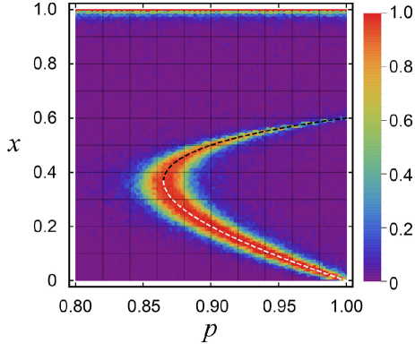
Therefore, for $p$ large enough, there may exist up to two strong SNE besides $(0,1)$ and $(1,0)$ that do not exist for small $p$. The results of stochastic simulations are shown in Fig. 1, and we can see that these results exactly match the theoretical predictions.

Figure 1: Stochastic simulation results for the existence of a strong SNE in the example. We take $b=10$, $c=4$ and $\mu=0.01$ in the simulations. The horizontal axis denotes the value of $p$, and the vertical axis the initial strategy $\mathbf{x}=(x,1-x)$ in the population. At each time step, a randomly generated mutant strategy $\mathbf{v}=(v,1-v)$ for $v\in[0,1]$ will randomly appear in the population with probability $0.01$. The color of each point on the $p$ - $x$ plane represents the average proportion of the initial strategy in the population after $10^{4}$ time steps in $100$ runs. The black dashed curve, the white dashed curve and the boundary $x=1$ represent the theoretical predictions for three strong SNE strategies as functions of $p$.

Conclusion. Stochastic fluctuations (or uncertainty) in returns in a temporally varying environment could have a profound impact on the evolution of animal behavior. Therefore, introducing the concept of a stochastic Nash equilibrium (SNE) that extends the classical concept of a NE [2, 7] to take into account random payoffs and revealing its relationship with a stochastically evolutionarily stable (SES) strategy [8, 11] may be of prime interest.

For the definition of a SNE as the strategy that is the best reply to itself in a stochastic framework, we have to compare geometric rather than arithmetic mean payoffs of strategies. Moreover, the SNE is said weak in the case of an equality for all other strategies, while it is said strong if there is a strict inequality for all other strategies.

Considering a linear evolutionary game with a random payoff matrix $\mathbf{A}(t)$ at each time step $t\geq 1$ and using conditions for stochastic stability or instability of equilibria [8], we have shown that: (i) at least one SNE exists; (ii) a SES strategy must be a SNE; (iii) a strong SNE must be a SES strategy, but this is not necessarily the case for a weak SNE; and (iv) a strong SNE can be a completely mixed strategy, and more than one can exist.

The concept of a SNE defined in a stochastic framework not only fully covers the classical concept of a NE in a deterministic setting, but a SNE may have some properties that a NE cannot possess. For instance, in classical matrix games, a completely mixed strategy cannot be a strict NE (strong NE in our terminology), while a completely mixed NE must correspond to an interior equilibrium in the evolutionary dynamics of pure strategies [2, 7, 4]. On the contrary, a completely mixed strategy can be a strong SNE as shown in this paper, but it must not correspond to an interior constant equilibrium in the stochastic evolutionary dynamics of pure strategies [8, 10, 11].

The concept of a SNE, especially the existence of a completely mixed strong SNE that is noise-induced, may play an important role for a better understanding of the evolutionary complexity of animal behavior in natural populations subject to environmental noise, such as the evolution of cooperation in a stochastic environment [13, 14, 15]. This is also consistent with Maynard Smith’s [2] emphasis on the importance of mixed strategies in evolutionary games.

Appendix

Consider a population in which only two mixed strategies are in use, $\mathbf{u}=(u,1-u)$ and $\mathbf{v}=(v,1-v)$ with $u,v\in[0,1]$. The payoff matrix for these two mixed strategies at time step $t\geq 1$ is given by

$$\begin{pmatrix}\mathbf{u}\cdot\mathbf{A}(t)\mathbf{u}&\mathbf{u}\cdot\mathbf{A}(t)\mathbf{v}\\ \mathbf{v}\cdot\mathbf{A}(t)\mathbf{u}&\mathbf{v}\cdot\mathbf{A}(t)\mathbf{v}\end{pmatrix}\ .$$ (A1)

This appendix provides a detailed analysis for the existence of stochastic Nash equilibria as defined in Eq. (7) in the main text.

For convenience, we define

$$Q(u,v) =\left<\log\big{(}\mathbf{u}\cdot\mathbf{A}(t)\mathbf{v}\big{)}\right>\ .$$ (A2)

Note that the expression $\mathbf{u}\cdot\mathbf{A}(t)\mathbf{v}$ is a convex combination of the elements of the payoff matrix $\mathbf{A}(t)$ whose coefficients are $uv$, $u(1-v)$, $(1-u)v$ and $(1-u)(1-v)$, respectively, and that the entries of $\mathbf{A}(t)$ are positive random variables that are uniformly bounded below and above by some positive constants, that is, there exist real numbers $A$ and $B$ such that $0<A\leq a_{ij}(t)\leq B$ for all $i,j=1,2$ and $t\geq 1$. Thus, the function $\log\big{(}\mathbf{u}\cdot\mathbf{A}(t)\mathbf{v}\big{)}$ is continuous and differentiable with respect to $u$ and $v$. Moreover, the partial derivative of $Q(u,v)$ with respect to $u$ is given by

$$\frac{\partial Q(u,v)}{\partial u} =\frac{\partial\left<\log\big{(}\mathbf{u}\cdot\mathbf{A}(t)\mathbf{v}\big{)}\right>}{\partial u}$$

$$=\left<\frac{\partial\log\big{(}\mathbf{u}\cdot\mathbf{A}(t)\mathbf{v}\big{)}}{\partial u}\right>$$

$$=\left<\frac{\big{(}\mathbf{A}(t)\mathbf{v}\big{)}_{1}-\big{(}\mathbf{A}(t)\mathbf{v}\big{)}_{2}}{\mathbf{u}\cdot\mathbf{A}(t)\mathbf{v}}\right>\ .$$ (A3)

Similarly, the second-order partial derivative of $Q(u,v)$ with respect to $u$ exists and is given by

$$\frac{\partial^{2}Q(u,v)}{\partial u^{2}} =-\left<\frac{\big{[}\big{(}\mathbf{A}(t)\mathbf{v}\big{)}_{1}-\big{(}\mathbf{A}(t)\mathbf{v}\big{)}_{2}\big{]}^{2}}{\big{(}\mathbf{u}\cdot\mathbf{A}(t)\mathbf{v}\big{)}^{2}}\right>\ .$$ (A4)

Note also that $0<A^{2}\leq\big{(}\mathbf{u}\cdot\mathbf{A}(t)\mathbf{v}\big{)}^{2}\leq B^{2}$ and $\big{[}\big{(}\mathbf{A}(t)\mathbf{v}\big{)}_{1}-\big{(}\mathbf{A}(t)\mathbf{v}\big{)}_{2}\big{]}^{2}\geq 0$. Thus, we have

$$\frac{\partial^{2}Q(u,v)}{\partial u^{2}}\leq-\frac{1}{B^{2}}\left<\big{[}\big{(}\mathbf{A}(t)\mathbf{v}\big{)}_{1}-\big{(}\mathbf{A}(t)\mathbf{v}\big{)}_{2}\big{]}^{2}\right>\leq 0\ .$$ (A5)

We can conclude that $\partial^{2}Q(u,v)/\partial u^{2}=0$ if and only if $\mathbf{P}\left(\big{(}\mathbf{A}(t)\mathbf{v}\big{)}_{1}=\big{(}\mathbf{A}(t)\mathbf{v}\big{)}_{2}\right)=1$, in which case we have also $\partial Q(u,v)/\partial u=0$.

Two cases have to be considered.

Case 1. $v\in[0,1]$ is such that $\mathbf{P}\left(\big{(}\mathbf{A}(t)\mathbf{v}\big{)}_{1}=\big{(}\mathbf{A}(t)\mathbf{v}\big{)}_{2}\right)=1$, so that $\mathbf{u}\cdot\mathbf{A}(t)\mathbf{v}=\mathbf{v}\cdot\mathbf{A}(t)\mathbf{v}$ with probability $1$, from which

$$Q(u,v)-Q(v,v) =\left<\log\Big{(}\frac{\mathbf{u}\cdot\mathbf{A}(t)\mathbf{v}}{\mathbf{v}\cdot\mathbf{A}(t)\mathbf{v}}\Big{)}\right>=0$$ (A6)

for all possible $\mathbf{u}=(u,1-u)$ with $u\in[0,1]$. This implies that $\mathbf{v}=(v,1-v)$ is a weak SNE, but not a strong SNE as defined in the main text. Moreover, note that the above condition takes the form

$$\mathbf{P}\left(\big{(}a_{11}(t)-a_{21}(t)\big{)}v=\big{(}a_{22}(t)-a_{12}(t)\big{)}(1-v)\right)=1.$$ (A7)

A solution $v\in[0,1]$ that satisfies this condition involves four possible situations.

(i) $\mathbf{P}\big{(}a_{11}(t)=a_{21}(t)\big{)}=1$ and $\mathbf{P}\left(a_{22}(t)=a_{12}(t)\right)=1$, in which case every $v\in[0,1]$ is a solution.

(ii) $\mathbf{P}\big{(}a_{11}(t)=a_{21}(t)\big{)}=1$ and $\mathbf{P}\left(a_{22}(t)=a_{12}(t)\right)<1$, in which case $v=1$ is the unique solution.

(iii) $\mathbf{P}\left(a_{11}(t)=a_{21}(t)\right)<1$ and $\mathbf{P}\big{(}a_{22}(t)=a_{12}(t)\big{)}=1$, in which case $v=0$ is the unique solution.

(iv) $\mathbf{P}\left(a_{11}(t)=a_{21}(t)\right)<1$ and $\mathbf{P}\big{(}a_{22}(t)=a_{12}(t)\big{)}<1$, in which case $r>0$ satisfying $\mathbf{P}\big{(}a_{11}(t)-a_{21}(t)=r\left(a_{22}(t)-a_{12}(t)\right)\big{)}=1$ is unique if it exists, and then $v=1/(1+r)\in(0,1)$ is the unique solution.

As for stochastic local stability, it is known that, under the condition $\mathbf{u}\cdot\mathbf{A}(t)\mathbf{v}=\mathbf{v}\cdot\mathbf{A}(t)\mathbf{v}$ with probability $1$ in the payoff matrix (A1), the mixed strategy $\mathbf{v}$ is SLS against the mixed strategy $\mathbf{u}$ if

$$\left<\frac{\mathbf{v}\cdot\mathbf{A}(t)\mathbf{u}}{\mathbf{v}\cdot\mathbf{A}(t)\mathbf{v}}-\frac{\mathbf{u}\cdot\mathbf{A}(t)\mathbf{u}}{\mathbf{v}\cdot\mathbf{A}(t)\mathbf{v}}\right>=\left<\frac{\mathbf{v}\cdot\mathbf{A}(t)\mathbf{u}}{\mathbf{v}\cdot\mathbf{A}(t)\mathbf{v}}\right>-\left<\frac{\mathbf{u}\cdot\mathbf{A}(t)\mathbf{u}}{\mathbf{v}\cdot\mathbf{A}(t)\mathbf{v}}\right>>0$$ (A8)

and SLU if the inequality is reversed (see Eq. (15) in [8]). Besides, $\mathbf{v}$ is stochastically evolutionarily stable (SES) if it is SLS against all $\mathbf{u}\neq\mathbf{v}$.

Note that, using Eq. (A7) and introducing the notation $\mathbf{z}=(1,-1)$, we have almost surely

$$(\mathbf{v}-\mathbf{u})\cdot\mathbf{A}(t)\mathbf{u} =(v-u)\mathbf{z}\cdot\mathbf{A}(t)\mathbf{u}$$

$$=(v-u)\Big{[}u\big{(}a_{11}(t)-a_{21}(t)\big{)}+(1-u)\big{(}a_{12}(t)-a_{22}(t)\big{)}\Big{]}$$

$$=(v-u)\Big{[}u\big{(}a_{11}(t)-a_{21}(t)\big{)}-v\big{(}a_{11}(t)-a_{21}(t)\big{)}$$

$$\ \ \ \ \ \ \ +(1-u)\big{(}a_{12}(t)-a_{22}(t)\big{)}+(1-v)\big{(}a_{22}(t)-a_{12}(t)\big{)}\Big{]}$$

$$=-(v-u)^{2}\mathbf{z}\cdot\mathbf{A}(t)\mathbf{z}$$ (A9)

and

$$\big{(}\mathbf{z}\cdot\mathbf{A}(t)\mathbf{z}\big{)}^{2}\mathbf{v}\cdot\mathbf{A}(t)\mathbf{v}$$

$$=\big{(}a_{11}(t)-a_{12}(t)-a_{21}(t)+a_{22}(t)\big{)}^{2}$$

$$\quad\times\left[v^{2}a_{11}(t)+v(1-v)\left(a_{12}(t)+a_{21}(t)\right)+(1-v)^{2}a_{22}(t)\right]$$

$$=\left(a_{22}(t)-a_{12}(t)\right)^{2}a_{11}(t)+\left(a_{22}(t)-a_{12}(t)\right)\left(a_{11}(t)-a_{21}(t)\right)\left(a_{12}(t)+a_{21}(t)\right)$$

$$\quad+\left(a_{11}(t)-a_{21}(t)\right)^{2}a_{22}(t)$$

$$=\big{(}\mathbf{z}\cdot\mathbf{A}(t)\mathbf{z}\big{)}\det\mathbf{A}(t)\ ,$$ (A10)

where

$$\mathbf{z}\cdot\mathbf{A}(t)\mathbf{z}=a_{11}(t)-a_{12}(t)-a_{21}(t)+a_{22}(t)$$ (A11)

and $\det\mathbf{A}(t)=a_{11}(t)a_{22}(t)-a_{12}(t)a_{21}(t)$. Moreover, $\det\mathbf{A}(t)=0$ almost surely if $\mathbf{z}\cdot\mathbf{A}(t)\mathbf{z}=0$, since then $a_{22}(t)-a_{12}(t)=a_{11}(t)-a_{21}(t)=0$ almost surely. Therefore, Eq. (Appendix) can be replaced by

$$\big{(}\mathbf{z}\cdot\mathbf{A}(t)\mathbf{z}\big{)}\mathbf{v}\cdot\mathbf{A}(t)\mathbf{v}=\det\mathbf{A}(t)$$ (A12)

with $\det\mathbf{A}(t)=0$ if and only if $\mathbf{z}\cdot\mathbf{A}(t)\mathbf{z}=0$. We can conclude that

$$\left<\frac{\mathbf{v}\cdot\mathbf{A}(t)\mathbf{u}}{\mathbf{v}\cdot\mathbf{A}(t)\mathbf{v}}-\frac{\mathbf{u}\cdot\mathbf{A}(t)\mathbf{u}}{\mathbf{v}\cdot\mathbf{A}(t)\mathbf{v}}\right>=\left<\frac{(\mathbf{v}-\mathbf{u})\cdot\mathbf{A}(t)\mathbf{u}}{\mathbf{v}\cdot\mathbf{A}(t)\mathbf{v}}\right> =-(v-u)^{2}D\ ,$$ (A13)

where

$$D =\left<\frac{\big{(}\mathbf{z}\cdot\mathbf{A}(t)\mathbf{z}\big{)}^{2}}{\det\mathbf{A}(t)}\right>$$ (A14)

with the convention that $\big{(}\mathbf{z}\cdot\mathbf{A}(t)\mathbf{z}\big{)}^{2}/\det\mathbf{A}(t)=0$ when $\mathbf{z}\cdot\mathbf{A}(t)\mathbf{z}=\det\mathbf{A}(t)=0$. If $D<0$, then the inequality in Eq. (A8) holds for all $\mathbf{u}\neq\mathbf{v}$, which means that $\mathbf{v}$ is SES. On the contrary, this is not possible when $D>0$,

Case 2. $v\in[0,1]$ is such that $\mathbf{P}\left(\big{(}\mathbf{A}(t)\mathbf{v}\big{)}_{1}=\big{(}\mathbf{A}(t)\mathbf{v}\big{)}_{2}\right)<1$, from which

$$\left<\big{[}\big{(}\mathbf{A}(t)\mathbf{v}\big{)}_{1}-\big{(}\mathbf{A}(t)\mathbf{v}\big{)}_{2}\big{]}^{2}\right>>0,$$ (A15)

and then Eq. (A4) yields $\partial^{2}Q(u,v)/\partial u^{2}<0$. This means that $Q(u,v)$ is a strictly concave function with respect to $u\in[0,1]$, which then reaches a unique global maximum at some point

$$\phi(v)=\mathop{\arg\max}\limits_{u\in[0,1]}Q(u,v)\in[0,1]\ .$$ (A16)

On the other hand, it is known that the mixed strategy $\mathbf{v}$ is SLS if $Q(u,v)<Q(v,v)$, and SLU if the inequality is reversed (see Eq. (10) in [8]). Therefore, we have

$$Q(u,v)-Q(v,v) =\left<\log\Big{(}\frac{\mathbf{u}\cdot\mathbf{A}(t)\mathbf{v}}{\mathbf{v}\cdot\mathbf{A}(t)\mathbf{v}}\Big{)}\right>\leq 0$$ (A17)

with an equality to $0$ if and only if $\mathbf{u}=\mathbf{v}$, and then $\mathbf{v}$ is SES, only when $v=\phi(v)$. In this case, we have

$$\frac{\partial Q(u,v)}{\partial u}\Big{|}_{u=v}\begin{cases}\leq 0&\textrm{ if }v=0,\\ \geq 0&\textrm{ if }v=1,\\ =0&\textrm{ if }0<v<1,\end{cases}$$ (A18)

and $\mathbf{v}=(v,1-v)$ is a strong SNE as defined in the main text.

As for the existence of a strong SNE, two situations have to be considered.

(i) $\mathbf{P}\left(\big{(}\mathbf{A}(t)\mathbf{v}\big{)}_{1}=\big{(}\mathbf{A}(t)\mathbf{v}\big{)}_{2}\right)<1$ for all $v\in[0,1]$, so that $\phi(v)$ is well defined and continuous on $[0,1]$. Then, this is also the case for the function defined by $g(v)=\phi(v)-v$. Moreover, we have $g(0)=\phi(0)\geq 0$ and $g(1)=\phi(1)-1\leq 0$. According to the mean value theorem, there exists $v^{*}\in[0,1]$ such that $g(v^{*})=0$, that is, $\phi(v^{*})=v^{*}$. The corresponding mixed strategy $\mathbf{v^{*}}=(v^{*},1-v^{*})$ is then a strong SNE.

(ii) $\mathbf{P}\left(\big{(}\mathbf{A}(t)\mathbf{\hat{v}}\big{)}_{1}=\big{(}\mathbf{A}(t)\mathbf{\hat{v}}\big{)}_{2}\right)=1$ for some $\hat{v}\in[0,1]$, so that $\mathbf{\hat{v}}=(\hat{v},1-\hat{v})$ is a weak SNE since $Q(u,\hat{v})-Q(\hat{v},\hat{v})=0$ for all $u\in[0,1]$, in which case $\phi(\hat{v})=[0,1]$. From the analysis in Case 1, we know that $\hat{v}$ is unique if it exists unless $\mathbf{P}\big{(}a_{11}(t)=a_{21}(t)\big{)}=1$ and $\mathbf{P}\left(a_{22}(t)=a_{12}(t)\right)=1$, which is excluded here since we assume that there exists $v\in[0,1]$ such that $\mathbf{P}\left(\big{(}\mathbf{A}(t)\mathbf{v}\big{)}_{1}=\big{(}\mathbf{A}(t)\mathbf{v}\big{)}_{2}\right)<1$. Note also that, if $\hat{v}$ exists, then $\phi(v)$ is well defined and continuous on the intervals $[0,\hat{v})$ and $(\hat{v},1]$.

From Eqs. (Appendix) and (A11), we find that $F(u,v)=\partial Q(u,v)\big{/}\partial u$ has a partial derivative with respect to $v$ given by

$$\left<\frac{(\mathbf{z}\cdot\mathbf{A}(t)\mathbf{z})(\mathbf{u}\cdot\mathbf{A}(t)\mathbf{v})-\left(\big{(}\mathbf{A}(t)\mathbf{v}\big{)}_{1}-\big{(}\mathbf{A}(t)\mathbf{v}\big{)}_{2}\right)\left(\big{(}\mathbf{u}^{T}\mathbf{A}(t)\big{)}_{1}-\big{(}\mathbf{u}^{T}\mathbf{A}(t)\big{)}_{2}\right)}{\big{(}\mathbf{u}\cdot\mathbf{A}(t)\mathbf{v}\big{)}^{2}}\right>.$$ (A19)

Evaluating at $v=\hat{v}$ and using Eq. (A12) for the expression of $\mathbf{u}\cdot\mathbf{A}(t)\mathbf{\hat{v}}=\mathbf{\hat{v}}\cdot\mathbf{A}(t)\mathbf{\hat{v}}$, we get

$$\frac{\partial F(u,\hat{v})}{\partial v}=D$$ (A20)

with $D$ as defined in Eq. (A14), while we have $F(u,\hat{v})=0$ owing to Eq. (Appendix), for all $u\in[0,1]$.

If $D>0$ and $\hat{v}>0$, then $\partial F(1,\hat{v})/\partial v>0$ and there exists $\epsilon_{1}>0$ such that $F(1,v)<0$ for $v\in(\hat{v}-\epsilon_{1},\hat{v})$. On the other hand, from Eq. (A5) and the unicity of $\hat{v}$, the function $F(u,v)$ is strictly increasing with respect to $u$ for $v\neq\hat{v}$, which implies that $F(u,v)\leq F(1,v)<0$ for $u\in[0,1]$ and $v\in(\hat{v}-\epsilon_{1},\hat{v})$. This also implies that $Q(u,v)$ is a strictly decreasing function of $u$ whose maximum is reached at $u=0$ for $v\in(\hat{v}-\epsilon_{1},\hat{v})$, in which case $\phi(v)=0$. Therefore, we have $g(\hat{v}^{-})=\lim\limits_{v\uparrow\hat{v}}(\phi(v)-v)=-\hat{v}<0$, while $g(0)=\phi(0)\geq 0$. The mean value theorem applied to the continuous function $g(v)$ on $[0,\hat{v})$ ensures the existence of $v^{*}_{1}\in[0,\hat{v})$ such that $g(v^{*}_{1})=0$, that is, $\phi(v^{*}_{1})=v^{*}_{1}$. The corresponding mixed strategy $\mathbf{v}^{*}_{1}=(v^{*}_{1},1-v^{*}_{1})$ is then a strong SNE.

Analogously, if $D>0$ and $\hat{v}<1$, then we can find $\epsilon_{2}>0$ such that $F(u,v)\geq F(1,v)>0$ for $u\in[0,1]$ and $v\in(\hat{v},\hat{v}+\epsilon_{2})$, which implies $\phi(v)=1$. In this case, we have $g(\hat{v}^{+})=\lim\limits_{v\downarrow\hat{v}}(\phi(v)-v)=1-\hat{v}>0$, while $g(1)=\phi(1)-1\leq 0$. Therefore, there exists $v^{*}_{2}\in(\hat{v},1]$ such that $g(v^{*}_{2})=0$, that is, $\phi(v^{*}_{2})=v^{*}_{2}$, and the corresponding mixed strategy $\mathbf{v}^{*}_{2}=(v^{*}_{2},1-v^{*}_{2})$ is a strong SNE.

Note that, if $D>0$ and $\hat{v}\in(0,1)$, then there are at least three stochastic Nash equilibria, which are $\hat{\mathbf{v}}=(\hat{v},1-\hat{v})$, $\mathbf{v}^{*}_{1}=(v^{*}_{1},1-v^{*}_{1})$ and $\mathbf{v}^{*}_{2}=(v^{*}_{2},1-v^{*}_{2})$, respectively, with $v^{*}_{1}<\hat{v}<v^{*}_{2}$. Whereas $\hat{\mathbf{v}}$ is a SNE that is not SES (see Case 1), the mixed strategies $\mathbf{v}^{*}_{1}$ and $\mathbf{v}^{*}_{2}$ are both strong SNE and then necessarily SES.

Similarly, if $D>0$ and $\hat{v}=0$ or $1$, then there is at least one SNE apart from $\hat{v}$, which is a strong SNE, and then SES, contrary to $\hat{v}$.

If $D<0$, however, it is possible that there is no other SNE except for $\hat{\mathbf{v}}$, which is a weak SNE that is SES.

Finally, in the case where $D=0$, for which $\partial F(u,\hat{v})/\partial v=0$ for all $u\in[0,1]$, we consider the second-order partial derivative of $F(u,v)$ with respect to $v$ evaluated at $v=\hat{v}$, which is given by

$$\frac{\partial^{2}F(u,\hat{v})}{\partial v^{2}} =-2\left<\frac{(\mathbf{z}\cdot\mathbf{A}(t)\mathbf{z})\left(\big{(}\mathbf{u}^{T}\mathbf{A}(t)\big{)}_{1}-\big{(}\mathbf{u}^{T}\mathbf{A}(t)\big{)}_{2}\right)}{\big{(}\mathbf{u}\cdot\mathbf{A}(t)\mathbf{\hat{v}}\big{)}^{2}}\right>$$

$$=-2\left<\frac{(\mathbf{z}\cdot\mathbf{A}(t)\mathbf{z})^{3}\left(\big{(}\mathbf{u}^{T}\mathbf{A}(t)\big{)}_{1}-\big{(}\mathbf{u}^{T}\mathbf{A}(t)\big{)}_{2}\right)}{\big{(}\det\mathbf{A}(t)\big{)}^{2}}\right>$$ (A21)

owing to Eqs. (A19) and (A12) with the convention that $\big{(}\mathbf{z}\cdot\mathbf{A}(t)\mathbf{z}\big{)}^{3}/(\det\mathbf{A}(t))^{2}=0$ when $\mathbf{z}\cdot\mathbf{A}(t)\mathbf{z}=\det\mathbf{A}(t)=0$. Defining

$$G =\left<\frac{(\mathbf{z}\cdot\mathbf{A}(t)\mathbf{z})^{3}}{\big{(}\det\mathbf{A}(t)\big{)}^{2}}\big{(}a_{11}(t)-a_{12}(t)\big{)}\right>\ ,$$ (A22a)

$$H =\left<\frac{(\mathbf{z}\cdot\mathbf{A}(t)\mathbf{z})^{3}}{\big{(}\det\mathbf{A}(t)\big{)}^{2}}\big{(}a_{21}(t)-a_{22}(t)\big{)}\right>\ ,$$ (A22b)

we find that

$$G-H =\left<\frac{(\mathbf{z}\cdot\mathbf{A}(t)\mathbf{z})^{4}}{\big{(}\det\mathbf{A}(t)\big{)}^{2}}\right>>0.$$ (A23)

Here, we use the fact $\mathbf{P}\left(\mathbf{z}\cdot\mathbf{A}(t)\mathbf{z}=0\right)<1$, since it is assumed that there exists $v\in[0,1]$ such that $\mathbf{P}\left(\big{(}\mathbf{A}(t)\mathbf{v}\big{)}_{1}=\big{(}\mathbf{A}(t)\mathbf{v}\big{)}_{2}\right)<1$. Moreover, we have

$$\frac{d^{2}F(u,\hat{v})}{dv^{2}}=-2\big{[}uG+(1-u)H\big{]}$$ (A24)

for $u\in[0,1]$.

There are three cases to consider:

1. if $0\leq H<G$, then we have $d^{2}F(u,\hat{v})/dv^{2}<0$ for $u\in(0,1]$, from which $\phi(\hat{v}^{-})=\lim\limits_{v\uparrow\hat{v}}\phi(v)=0$ if $\hat{v}>0$ and $\phi(\hat{v}^{+})=\lim\limits_{v\downarrow\hat{v}}\phi(v)=0$ if $\hat{v}<1$, since then $F(u,v)\leq F(1,v)<0$ for $u\in(0,1]$ and $\phi(v)=0$ for $v\neq\hat{v}$ close enough to $\hat{v}$;

2. if $H<G\leq 0$, then we have $d^{2}F(u,\hat{v})/dv^{2}>0$ for $u\in[0,1)$, from which $\phi(\hat{v}^{-})=1$ if $\hat{v}>0$ and $\phi(\hat{v}^{+})=1$ if $\hat{v}<1$ by symmetry with the previous case with $F(u,v)\geq F(0,v)>0$ for $u\in[0,1)$ and $\phi(v)=1$ for $v\neq\hat{v}$ close enough to $\hat{v}$; and

3. if $G>0>H$, then we have $d^{2}F(\hat{u},\hat{v})/dv^{2}=0$ for $\hat{u}=H\big{/}(H-G)\in(0,1)$, while $d^{2}F(u,\hat{v})/dv^{2}<0$ for $u\in(\hat{u},1]$ and $d^{2}F(u,\hat{v})/dv^{2}>0$ for $u\in[0,\hat{u})$, from which $\phi(\hat{v}^{-})=\phi(\hat{v}^{+})=\hat{u}$ by analogy with the two previous cases.

Now, let us define $g(v)=\phi(v)-v$ for $v\neq\hat{v}$ and

$$g(\hat{v})=\begin{cases}-\hat{v}&\textrm{ if }\hat{u}\leq 0,\\ 1-\hat{v}&\textrm{ if }\hat{u}\geq 1,\\ \hat{u}-\hat{v}&\textrm{ if }\hat{u}\in(0,1).\end{cases}$$ (A25)

This is a continuous function on $[0,1]$ in the three cases above with $g(0)\geq 0$ and $g(1)\leq 0$. Moreover, applying the mean value theorem, there exist $v^{*}_{1}\in[0,\hat{v})$ such that $g(v^{*}_{1})=0$ if $\hat{v}>\max(0,\hat{u})$, as well as $v^{*}_{2}\in(\hat{v},1]$ such that $g(v^{*}_{2})=0$ if $\hat{v}<\min(1,\hat{u})$. The corresponding mixed strategies $\mathbf{v}^{*}_{1}=(v^{*}_{1},1-v^{*}_{1})$ and $\mathbf{v}^{*}_{2}=(v^{*}_{2},1-v^{*}_{2})$ are strong SNE, while $\mathbf{\hat{v}}=(\hat{v},1-\hat{v})$ is a SNE that is not SES.

We now give an example to show the nature of the function $\phi(v)$ according to the sign of $D$.

Example A1. Consider a random payoff matrix

$$\mathbf{A}(t)=\begin{pmatrix}c+r\eta_{t}&b\\ c&b+\eta_{t}\end{pmatrix}\ ,$$ (A26)

where $b,c,r$ are positive constants, and

$$\eta_{t}=\begin{cases}s&\textrm{ with probability }p\ ,\\ -s&\textrm{ with probability }1-p\ ,\end{cases}$$ (A27)

with $0<s<\min(b,c/r)$. It is easy to show that $(\hat{v},1-\hat{v})$ with $\hat{v}=1/(1+r)\in(0,1)$ is a unique weak SNE. Moreover, from Eq. (A14), we have

$$D =\left<\frac{(r+1)^{2}\eta_{t}}{c+rb+r\eta_{t}}\right>=s\frac{(2p-1)(c+rb)-rs}{(c+rb)^{2}-r^{2}s^{2}}\ .$$ (A28)

Since $c+rb>rs$, we can see that the sign of $D$ corresponds to the sign of $(2p-1)(c/r+b)-s$. Moreover,

$$F(u,v) =\frac{\partial Q(u,v)}{\partial u}=\frac{v-\hat{v}}{\hat{v}}\left<\frac{\eta_{t}}{\mathbf{u}\cdot\mathbf{A}(t)\mathbf{v}}\right>$$

$$=\frac{v-\hat{v}}{\hat{v}}\left<\frac{\eta_{t}}{(vc+(1-v)b)+(uvr+(1-u)(1-v))\eta_{t}}\right>\ .$$ (A29)

By solving the equation $F(u,v)=0$ for $v\neq\hat{v}$, which can be simplified to a one-dimensional equation, we get

$$\phi(v) =\begin{cases}\min\left(1,\max\left(0,\frac{((2p-1)(c-b)+s)v+(2p-1)b-s}{s(r+1)v-s}\right)\right)&\textrm{ for }v\neq\hat{v}\ ,\\ [0,1]&\textrm{ for }v=\hat{v}\ .\end{cases}$$ (A30)

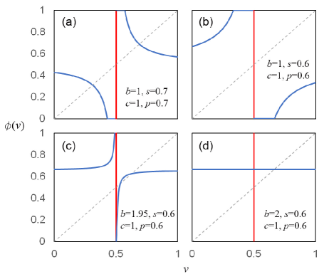
If $D>0$, then $\phi(v)$ has at least two intersection points with the line $\phi(v)=v$ that correspond to two strong SNE (see Fig. A1a). If $D<0$, then a strong SNE may exist or not (see Fig. A1b and A1c). On the other hand, if $D=0$, which means that $s=(2p-1)(c/r+b)$, then $\phi(v)$ becomes the constant $c/(c+rb)=\hat{u}\in(0,1)$ for $v\neq\hat{v}$. If $\hat{u}\neq\hat{v}$, that is, $b\neq c$, then we can always find a strong SNE given by $(\hat{u},1-\hat{u})$. In this case, the mixed strategy $(\hat{u},1-\hat{u})$ is the unique best reply to any other strategy, except for $(\hat{v},1-\hat{v})$, with respect to the geometric means of the payoffs (see Fig. A1d). If $b=c$, then $(\hat{v},1-\hat{v})$ is the unique SNE in the system.

Figure A1: The function $\phi(v)$ in Example A1

Example A2. In this example, we consider a random payoff matrix

$$\mathbf{A}(t)=\begin{pmatrix}c+(1-a)(1-\hat{v})\eta_{t}&b-(1-a)\hat{v}\eta_{t}\\ c-a(1-\hat{v})\eta_{t}&b+a\hat{v}\eta_{t}\end{pmatrix}\ ,$$ (A31)

where $b,c$ are positive constants and $a,\hat{v}\in(0,1)$, while $\eta_{t}$ is any non-constant white noise with $\left<\eta_{t}\right>=0$ that makes the entries in $\mathbf{A}(t)$ always positive (for instance, $|\eta_{t}|<\delta$, where $\delta>0$ is small enough). It is still easy to see that $(\hat{v},1-\hat{v})$ is the unique weak SNE. From Eq.(A14), we get

$$D =\left<\frac{(1-2\hat{v})^{2}}{(1-\hat{v})b+\hat{v}c}\eta_{t}\right>=\frac{(1-2\hat{v})^{2}}{(1-\hat{v})b+\hat{v}c}\left<\eta_{t}\right>=0$$ (A32)

almost surely, and

$$F(u,v) =(v-\hat{v})\left<\frac{\eta_{t}}{\mathbf{u}\cdot\mathbf{A}(t)\mathbf{v}}\right>$$

$$=(v-\hat{v})\left<\frac{\eta_{t}}{(v-\hat{v})(u(1-2a)-a)\eta_{t}+c\hat{v}+b(1-\hat{v})}\right>\ .$$ (A33)

When $a\in(0,1/3)$, we have $\hat{u}=a/(1-2a)\in(0,1)$ and $F(\hat{u},v)=\frac{v-\hat{v}}{c\hat{v}+b(1-\hat{v})}\left<\eta_{t}\right>=0$, from which $\phi(v)=\hat{u}$ for $v\neq\hat{v}$. This corresponds to the case where $D=0$, $G>0>H$. When $a\in[1/3,1/2)$, we have $\hat{u}=1$ and this corresponds to the case where $D=0$, $0\leq H<G$. Finally, when $a\in(1/2,1)$, we have $\hat{u}=0$, which corresponds to the case where $D=0$, $H<G\leq 0$.

References

[1] J. F. Nash, Equilibrium points in -person games. Proceedings of the National Academy of Sciences36(1): 48-49 (1950).
[2] J. Maynard Smith, Evolution and the Theory of
Games (Cambridge University Press, Cambridge, England, 1982).
[3] J. W. Weibull, Evolutionary Game Theory (MIT Press, Cambridge, Massachusetts, 1997).
[4] M. Broom and J. Rychtář, Game-Theoretical Models in Biology (2nd Edition) (Chapman and Hall/CRC, New York, 2022).
[5] J. Maynard Smith and G. R. Price, The logic of animal conflict. Nature246(5427): 15-18 (1973).
[6] J. Maynard Smith, The theory of games and the evolution of animal conflicts. Journal of Theoretical
Biology47(1): 209-221 (1974).
[7] J. Hofbauer and K. Sigmund, Evolutionary Games and Population Dynamics (Cambridge University Press, Cambridge, England, 1998).
[8] X.-D. Zheng, C. Li, S. Lessard and Y. Tao, Evolutionary stability concepts in a stochastic
environment. Physical Review E96: 032414 (2017).
[9] X.-D. Zheng, C. Li, S. Lessard and Y. Tao, Environmental noise could promote stochastic local stability
of behavioral diversity evolution. Physical Review Letters120: 218101 (2018).
[10] T.-J. Feng, J. Mei, R.-W. Wang, S. Lessard, Y. Tao and X.-D. Zheng, Noise-induced quasi-heteroclinic cycle in a rock-paper-scissors game with random payoffs. Dynamic Games and Applications12: 1280-1292 (2022).
[11] T.-J. Feng, C. Li, X.-D. Zheng, S. Lessard and Y. Tao, Stochastic replicator dynamics and evolutionary stability. Physical Review E105: 044403 (2022).
[12] M. A. Nowak, Evolutionary Dynamics (Harvard University Press,
Cambridge, Massachusetts, 2006).
[13] T.-J. Feng, S.-J. Fan, C. Li, Y. Tao, X.-D. Zheng, Noise-induced sustainability of cooperation in Prisoner’s Dilemma game. Applied Mathematics and Computation438: 127603 (2023).
[14] Y. Berbeg-Meyer, A.E. Roth, The speed of learning in noisy games: partial reinforcement and the sustainability of cooperation. American Economic Review96: 1029-1042 (2006).
[15] M. Perc, Coherence resonance in a spatial Prisoner’s Dilemma game. New Journal of Physics8: 22 (2006).