Existence of solution to a system of PDEs modeling the crystal growth inside lithium batteries

Tóm tắt n$\operatorname{d}\!$ôi dung.

The life of electric batteries depend on a complex system of interacting electrochemical and growth phenomena that produce dendritic structures during the discharge cycle. We study herein a system of 3 partial differential equations combining an Allen–Cahn phase-field model (simulating the dendrite-electrolyte interface) with the Poisson–Nernst–Planck systems simulating the electrodynamics and leading to the formation of such dendritic structures. We prove novel existence, uniqueness and stability results for this system and use it to produce simulations based on a finite element code.

1. Introduction

As humanity aims at reaching “net-zero” by 2050, replacing fossil fuels with renewable alternatives has spurred the research in storage technologies. One of the favored technologies, the lithium battery is the object of intense scrutiny by scientists and engineers (Akolkar, b; Chen et al., b; Cogswell, ; Ely et al., ; Hong and Viswanathan, ; Mu et al., a; Okajima et al., ; Yurkiv et al., , e.g.). One of the important phenomena in a Li-metal battery, i.e., a battery with a metallic lithium electrode, is the electrodeposition process during which solid structures known as dendrites may grow attached to the electrode into the electrolyte solution and lead to the battery’s deterioration and ultimately its failure (Okajima et al., ; Akolkar, a; Liang and Chen, ; Chen et al., b; Yurkiv et al., ). Our aim herein is a rigorous analytical and computational study of a partial differential equation (PDE) based model that describes the electrodeposition process and captures the dynamics of resulting dendritic growth phenomena. The model we study consolidates various models already addressed by the enginnering community (Chen et al., b; Liang and Chen, ; Liang et al., ), with some modifications resulting in a system of PDEs which we rigorously prove to be well-posed. The resulting system, which we fully describe in section 2.1, is captured by three interacting PDEs:

1. a nonlinear anisotropic Allen–Cahn equation, thus phase-field type PDE, with a forcing term that accounts for the Butler–Volmer electrochemical reaction kinetics, which models the concentration of Li atoms;

2. a reaction–diffusion Nernst–Planck equation, which describes the dynamics of the concentration of Li+;
   and

3. a Poisson type equation that describes the electric potential that drives the dynamics of the Li+ ions.

An early application of phase-field modeling to electrochemistry was introduced in Guyer et al. (a). In this work a new model was proposed, derived by a free energy functional that includes the electrostatic effect of charged particles leads to rich interactions between concentration, electrostatic potential and phase stability. This model was further studied by the same people in Guyer et al. (c, b). These papers gave motivation, mostly to engineers, to study the model and use it to describe lithium batteries. There is extensive literature with papers using variations of the model described by Guyer et al. (a) together with numerical simulations that are trying to capture the behavior of the Li-ion or Li-metal batteries in two spatial dimensions (Okajima et al., ; Liang et al., ; Akolkar, a; Zhang et al., a; Liang and Chen, ; Ely et al., ; Akolkar, b; Chen et al., b; Cogswell, ; Yurkiv et al., ; Hong and Viswanathan, ; Liu and Guan, ; Mu et al., a, e.g.) and in three (Mu et al., b, e.g.), using a Nernst–Planck–Poisson system coupled with an anisotropic phase-field equation.

The study of anisotropy in surfaces and interfaces goes back many decades, for example, in Hoffman and Cahn , a vector function was introduced as an alternative to the scalar function with which the anisotropic free energy of surfaces was usually described. Kobayashi pioneered research on anisotropic dendritic crystal growth phenomena since the mid 80s. He first introduced an anisotropic phase-field model to show the minimal set of factors which can yield a variety of typical dendritic patterns. This and later works were focused more on the solidification of pure material in two and three spatial dimensions (Kobayashi, a, b). The proposed model was proven to be able to describe realistic dendritic patterns numerically. In two spatial dimensions, the anisotropy occurs from the derivation of the energy. In three spatial dimensions, though, the anisotropy was given by an artificial term rather than from the deriviation of the energy, in order to reduce significantly the computational cost of the phase-field equation. Other works address numerical simulations more thoroughly for two spatial dimensions in Wheeler et al. . A better attempt on numerical simulations in three spatial dimensions was shown in Karma and Rappel . It was the first attempt that actually computed the anisotropic diffusion tensor. It was not until 1993 that analytical results on these models were established. In McFadden et al. an asymptotic analysis in the sharp-interface limit of the model studied in Kobayashi (a); Wheeler et al. was established, including an anisotropic mobility. In Wheeler and McFadden , a $\xi$-vector formulation of anisotropic phase-field models was introduced, as in Hoffman and Cahn , in an attempt to investigate the free-boundary problem approached in the sharp interface limit of the phase-field model used to compute three-dimensional dendrites. Mathematical analysis on different viewpoints of the former mentions, yet significantly useful on expanding the knowledge on the anisotropic phase-field models, has been developed in Elliott and Schätzle (a, b); Taylor and Cahn . In the early 2000s, there were three papers, Burman and Rappaz ; Burman et al. ; Burman and Picasso , that treated a coupled system of PDEs, including a phase-field equation with anisotropy, based on the model that was proposed by Warren and Boettinger for the dendritic growth and microsegregation patterns in a binary alloy at constant temperature. However, the proposed anisotropic diffusion tensor was implemented specifically for two spatial dimensions and so the analytical and numerical results were restricted in $\mathbb{R}^{2}$. In Graser et al. the same model was studied and the analytical results were expanded in three spatial dimensions. In the same paper different time discretizations were studied for their stability. A 3D implementation of the anisotropy was introduced considering the regularized $\ell^{1}$-norm (Graser et al., , Example 2.2), yet different than in Karma and Rappel , where the 3D anisotropy is given under the same principles that Kobayashi first introduced. More recently, in Li et al. new numerical schemes were introduced, but the numerical results that were presented were in two spatial dimensions. The study of the anisotropic phase-field equations is still in progress and one crucial challenge is the development of efficient numerical algorithms for three spatial dimensions. In Zhang et al. (b) numerical algorithms for the anisotropic Allen–Cahn equation with precise nonlocal mass conservation were proposed in this direction.

To our best knowledge, there are no rigorous analysis results for the system of PDEs. The Nernst–Planck–Poisson system is often coupled with the Navier-Stokes equation (Zhang and Yin, ; Bothe et al., , e.g.), or studied on its own (Kato, ; Chen et al., a, e.g.). In one occasion, Liu and Eisenberg , the proposed model, called Poisson–Nernst–Planck–Fermi, is replacing the Poisson equation with a fourth order Cahn–Hilliard type PDE, but it is not sharing many similarities with the model in this paper. The purpose of this work is to establish well-posedness results for the Nernst–Planck–Poisson system, coupled with the anisotropic phase-field equation, and to provide with numerical simulations of the dendritic crystal growth.

Our goal in this paper, is to show that the Nernst–Planck–Poisson system, coupled with the anisotropic phase-field equation, that was introduced in Liang et al. ; Liang and Chen ; Chen et al. (b), is well posed. A source of techniques we use is found in Burman and Rappaz . The difference in our paper is that the solution of the Poisson equation is used to give the vector field in the convection term of the convection-diffusion PDE, in comparison with the model of Burman and Rappaz where they produce the vector field from the solution of the phase-field equation. We have also added forcing terms to our reaction-diffusion PDE and to the Poisson equation, which are dependent on the order parameter. Our forcing term in the Allen–Cahn PDE is also coming from the Butler–Volmer electrochemical reaction kinetics, which give quite different numerical simulations both at the isotropic and the anisotropic cases. For more details, see Section 5.

The remainder of this paper is organised as follows. In Section 2 we present a rescaling of the equations (2.1a),(2.1b) and (2.1c), as well as a weak formulation of the system. We also introduce the anisotropy tensor and its properties. In Section 3 we will present the main result of this paper which is an existence result, using the Rothe’s method, for a weak solution of the system. In Section 5 we present some numerical simulations.

2. The PDE model and its weak formulation

In this section we present the model for the Lithium batteries. In Section 2.1 we start by presenting the equations that consist our PDE system. In Section 2.2 we “nondimensionalize” the model, so that we work without units and perform correct and efficient computations later. In Section 2.3 we pass to a weak formulation of the model. In Section 2.4 we introduce the anisotropic diffusion tensor, its derivation and useful properties. At last, we present the main result of this paper, in Section 2.5.

2.1. A Nernst–Planck–Poisson–Allen–Cahn model for Lithium batteries

Hình 1. A diagrammatic view of a Lithium battery represented by $\Omega=\left(0,L_{1}\right)\times B$

Let $\Omega\subseteq\mathbb{R}^{d},d=2,3$, be a bounded domain with Lipschitz boundary and $[0,T^{*}]$ is the time interval, with $T^{*}>0$ being a target “final” time. The model under study consists of an initial–boundary value problem for the three unknowns $u,c,\phi:\Omega\times\left[0,T^{*}\right]\to\mathbb{R}$ respectively indicating the phase-field variable (denoting the concentration of crystallized Li atoms), the concentration of Li+ ions, and the electric potential. The model we consider is an adjusted version of the model that was introduced in Chen et al. (b). Our addition is a relaxation parameter, denoted by $\epsilon$, which is useful for keeping the numerical results in the appropriate range of values. The rest remain the same, but with a different set of values. See Section 5 for more information on the numerical results. The model takes the form:

$$\epsilon^{2}\partial_{t}u=\nabla\cdot[\boldsymbol{{A}}(\nabla u)\nabla u]-\gamma g^{\prime}(u)-\kappa h^{\prime}(u)\big{(}\operatorname{e}\!^{\frac{(1-\alpha)nF\eta_{a}}{RT}}-c\operatorname{e}\!^{\frac{-\alpha nF\eta_{a}}{RT}}\big{)},$$ (2.1a)

$$\partial_{t}c=\nabla\cdot\big{[}D(u)\nabla c+D_{1}(u,c)\frac{nF}{RT}\nabla\phi\big{]}-\mu\partial_{t}u,$$ (2.1b)

$$\nabla\cdot\big{[}\sigma(u)\nabla\phi\big{]}=nFc_{s}\partial_{t}u,$$ (2.1c)

in $\Omega\times[0,T^{*}]$, where $\gamma,\kappa,\mu>0$, $\alpha\in[0,1]$ is a parameter that affects the symmetry of the magnitude of the forcing term in (2.1a), $n,F,R,T$ respectively are the valence of the chemical reaction of the Li^+ with the electrons e^-, the Faraday number, the gas constant and the temperature. The activation overpotential is given by $\eta_{a}$ and it is negative, $c_{s}>0$ represents the site density of Li-metal, $g,h,\sigma$ and $D$ are continuously differentiable functions and represent the double-well potential, the primitive of the double-well potential, the effective conductivity and the effective diffusion coefficient respectively and are formulated as follows,

$$g(s)=\left\{\begin{array}[]{ll}s^{2}(1-s)^{2}/4,&0\leq s\leq 1,\\ 0,&\text{elsewhere},\end{array}\right.$$ (2.4)

$$h(s)=\left\{\begin{array}[]{ll}1,&s>1,\\ s^{3}(6s^{2}-15s+10),&0\leq s\leq 1,\\ 0,&s<0,\end{array}\right.$$ (2.8)

$$D(s)=D^{\text{e}}h(s)+D^{\text{s}}(1-h(s))\text{ for }s\in\mathbb{R},$$ (2.9)

$$\sigma(s)=\sigma^{\text{e}}h(s)+\sigma^{\text{s}}(1-h(s))\text{ for }s\in\mathbb{R},$$ (2.10)

where $D^{\text{e}},D^{\text{s}}>0$ are the diffusion in the electrode and the electrolyte solution respectively. The same applies to $\sigma^{\text{e}},\sigma^{\text{s}}>0$ for the conductivity. The double-well potential and its primitive are Lipschitz continuous functions in the way they are defined. The effective diffusion and conductivity functions are also monotone functions when $0\leq u\leq 1$. The fact that the above coefficients are positive imply that these functions are also positive for these values of $u$. Also, we define $D_{1}:\mathbb{R}^{2}\to\mathbb{R}$ as

$$D_{1}(w,s)=\left\{\begin{array}[]{ll}D_{\min},&s>1,\\ D(w)s,&0\leq s\leq 1,\\ 0,&s<0,\end{array}\right.$$ (2.11)

where $D_{\min}:=\min_{s\in\mathbb{R}}D(s)$.

Although our analysis applies to general domains, $\Omega$, we will focus on the specific cylindirical geometry $\Omega=[0,L_{1}]\times B\subset\mathbb{R}^{d}$, $d=2,3$, with $L_{1}>0$, $B\in\mathbb{R}^{d-1}$, e.g., $B:=[0,L_{2}]^{d-1}$ for some $L_{2}>0$ and boundary $\partial\Omega=\Gamma_{1}\cup\Gamma_{2}\cup\Gamma^{\prime}$, with $\Gamma_{1},\Gamma_{2}$ representing the segments of the boundary where we consider (sometimes two different) Dirichlet boundary conditions, and $\Gamma^{\prime}$ where we take Neumann boundary conditions. In particular, in $d=2$, we have

$$\Gamma_{1}:=\left\{\boldsymbol{x}=(x,\boldsymbol{y})\in\Omega:\;x=0\right\},$$ (2.12)

$$\Gamma_{2}:=\left\{\boldsymbol{x}=(x,\boldsymbol{y})\in\Omega:\;x=L_{1}\right\}$$ (2.13)

$$\Gamma:=\Gamma_{1}\cup\Gamma_{2}\text{ and }\Gamma^{\prime}=\partial\Omega\smallsetminus\Gamma.$$ (2.14)

The boundary conditions for (2.1a),(2.1b) and (2.1c) are the following,

$$\operatorname{\mathbf{n}}_{\Omega}\cdot\boldsymbol{{A}}(\nabla u)\nabla u=0\text{ on }\partial\Omega\times[0,T^{*}],$$ (2.15a)

$$\operatorname{\mathbf{n}}_{\Omega}\cdot D(u)\nabla c=\operatorname{\mathbf{n}}_{\Omega}\cdot D_{1}(u,c)\nabla\phi\text{ on }\partial\Omega\times[0,T^{*}],$$ (2.15b)

$$\begin{split}\operatorname{\mathbf{n}}_{\Omega}\cdot\sigma(u)\nabla\phi=0&\text{ on }\Gamma^{\prime}\times[0,T^{*}],\\ \phi=\phi_{-}&\text{ on }\Gamma_{1}\times[0,T^{*}],\\ \phi=0&\text{ on }\Gamma_{2}\times[0,T^{*}],\end{split}$$ (2.15c)

with $\phi_{-}\in[-2,0)$ and $\operatorname{\mathbf{n}}_{\Omega}$ denoting the outward normal vector to $\Omega$. For the equation (2.1b) we use the natural boundary conditions. Since the system is time dependent, we need to implement initial values for the order parameter and the concentration of Li^+. We choose

$$u(\boldsymbol{x},0)=u_{0}(\boldsymbol{x})\text{ in }\Omega$$ (2.16a)

$$c(\boldsymbol{x},0)=c_{0}(\boldsymbol{x})\text{ in }\Omega$$ (2.16b)

so that $|u_{0}(\boldsymbol{x})|\leq 1$ and $|c_{0}(\boldsymbol{x})|\leq 1$.

2.2. Rescaling

We now rescale, by “nondimensionalizing” it, the system of PDEs (2.1a)–(2.1c), to ease the mathematical analysis and the associated numerical simulations.

We start with the rescaling of the system (2.1a)-(2.1c) . We set $\tilde{T}=T^{*}/\Delta t_{0}$ and $\tilde{L}_{i}=L_{i}/l_{0},\,i=1,2$, where $l_{0},\Delta t_{0}$ are length and time reference values for the model and using Table 1 in Chen et al. (b) we define,

$$\boldsymbol{x}=l_{0}\tilde{\boldsymbol{x}},\,t=\Delta t_{0}\tilde{t},\,D(u)=\frac{l_{0}^{2}}{\Delta t_{0}}\tilde{D}(u),\,\sigma(u)=\frac{l_{0}^{2}c_{0}F^{2}}{\Delta t_{0}RT}\tilde{\sigma}(u),\\ \phi=\frac{RT}{F}\tilde{\phi},\,\nabla\phi=\frac{RT}{l_{0}F}\nabla\tilde{\phi},\,\Delta\phi=\frac{RT}{l_{0}^{2}}\Delta\tilde{\phi},$$ (2.17)

$$\tilde{\Omega}\times[0,\tilde{T}]=[0,\tilde{L}_{1}]\times[0,\tilde{L}_{2}]\times[0,\tilde{T}].$$ (2.18)

We introduce the following coefficients

$$C_{1}=\kappa\operatorname{e}\!^{-(1-a)nF|\eta_{a}|/RT}$$ (2.19a)

$$C_{2}=\kappa\operatorname{e}\!^{anF|\eta_{a}|/RT}.$$ (2.19b)

For the consistency of our problem, we consider the following cutoff function of the coefficient of the forcing term

$$m(c)=\left\{\begin{array}[]{ll}C_{1}-C_{2},&c>1,\\ C_{1}-cC_{2},&0\leq c\leq 1,\\ C_{1},&c<0.\end{array}\right.$$ (2.20)

Using the above rescaling, and dropping the tilde notation for ease of presentation, the dimensionless form of (2.1a)–(2.1c) is given by

$$\epsilon^{2}\partial_{t}u=\nabla\cdot[\boldsymbol{{A}}(\nabla u)\nabla u]-\gamma g^{\prime}(u)+m(c)h^{\prime}(u) \text{ in }\Omega\times[0,T],$$ (2.21a)

$$\partial_{t}c=\nabla\cdot\big{[}D(u)\nabla c+D_{1}(u,c)\nabla\phi\big{]}-\mu\partial_{t}u \text{ in }\Omega\times[0,T],$$ (2.21b)

$$\nabla\cdot\big{[}\sigma(u)\nabla\phi\big{]}=\nu_{1}\partial_{t}u \text{ in }\Omega\times[0,T],$$ (2.21c)

together with the initial and boundary data (2.15a)–(2.15c) and (2.16a)–(2.16b).

2.3. The weak formulation

We next reformulate system the NPPAC system of 2.1 in weak form. To this aim, we briefly recall the functional space set-up, refering for details to standard texts (e.g. Evans, ). We write $\operatorname{L}_{p}(Q;\mathscr{{X}})$, for an open domain $Q\in\mathbb{R}^{q}$ and a normed vector space $\mathscr{{X}}$, as the space of (Lebesgue) $p$-summable functions $\varphi:Q\to\mathscr{{X}}$, equipped with a norm such that $\left\|{\varphi}\right\|_{\operatorname{L}_{p}(Q;\mathscr{{X}})}^{p}:=\int_{Q}\left\|{\varphi}\right\|_{\mathscr{{X}}}^{p}$. We write $\operatorname{L}_{p}(Q)^{k}$ when $\mathscr{{X}}=\mathbb{R}^{k}$. When $p=2$ and $\mathscr{{X}}$ has an inner product, the space $\operatorname{L}_{2}(Q;\mathscr{{X}})$ is also equipped with inner product $\left({\varphi,\psi}\right)_{\operatorname{L}_{2}(Q;\mathscr{{X}})}:=\int_{Q}\left({\varphi,\psi}\right)_{\mathscr{{X}}}$ for each $\varphi,\psi\in\operatorname{L}_{2}(Q;\mathscr{{X}})$. Generalising, we denote Sobolev spaces of weakly differentiable functions $\phi:Q\to\mathscr{{X}}$ up to order $m\in\mathbb{N}$ with $p$-summable derivatives by ${\smash{\operatorname{W}}}^{m}_{p}(Q;\mathscr{{X}})$ with leading seminorm $\left|\phi\right|_{{\smash{\operatorname{W}}}^{m}_{p}(\Omega;\mathscr{{X}})}:=\|\operatorname{D}\!^{m}\phi\|_{\operatorname{L}_{p}(Q;\mathscr{{X}})}$ and full norm $\left\|{\phi}\right\|_{{\smash{\operatorname{W}}}^{m}_{p}(\Omega;\mathscr{{X}})}^{p}:=\sum_{j=0}^{m}\left|\phi\right|_{{\smash{\operatorname{W}}}^{j}_{p}(\Omega;\mathscr{{X}})}^{p}$. When $p=2$ we shorten notation ${\smash{\operatorname{W}}}^{m}_{2}(Q;\mathscr{{X}})$ to $\operatorname{H}^{m}(Q;\mathscr{{X}})$. As for the Lebesgue spaces, when $\mathscr{{X}}=\mathbb{R}^{k}$ we write ${\smash{\operatorname{W}}}^{m}_{p}(Q)^{k}$ and $\operatorname{H}^{m}(Q)^{k}$ and drop $k=1$. For a Hilbert Sobolev space with Dirichlet boundary condition on $\Sigma\subseteq\partial Q$ we write $\operatorname{H}^{m}_{0|\Sigma}(Q)$ and $\operatorname{H}^{m}_{0}(Q)$ if $\Sigma=\partial Q$.

First, we reformulate the nonhomogeneous Dirichlet boundary conditions for both (2.21b) and (2.21c). To this end we introduce the decomposition

$$\bar{\phi}=\phi-\phi_{-}(L_{1}-x/L_{1}).$$ (2.22)

It is clear that $\phi_{-}(L_{1}-x/L_{1})x$ has boundary conditions that coincide with the boundary conditions (2.15c) of $\phi$. A direct calculation leads to

$$\nabla\cdot\big{[}\sigma(u)\nabla((L_{1}-x/L_{1})\phi_{-})\big{]}=-\nu_{2}\sigma^{\prime}(u)\partial_{x}u,$$ (2.23)

where $\nu_{2}=(\phi_{-}/L_{1})$. So we get

$$\nabla\cdot\big{[}\sigma(u)\nabla\bar{\phi}\big{]}=\nu_{1}\partial_{t}u-\nu_{2}\sigma^{\prime}(u)\partial_{x}u \text{ in }\Omega\times[0,T],$$ (2.24)

$$\operatorname{\mathbf{n}}_{\Omega}\cdot\sigma(u)\nabla\bar{\phi}=0 \text{ on }\Gamma^{\prime}\times[0,T],$$

$$\bar{\phi}|_{\Gamma}=0 \text{ on }\Gamma\times[0,T].$$

For simplicity of presentation we drop the bar notation for $\phi$ and the system in its final form is the following:

$$\epsilon^{2}\partial_{t}u=\nabla\cdot[\boldsymbol{{A}}(\nabla u)\nabla u]-\gamma g^{\prime}(u)+m(c)h^{\prime}(u) \text{ in }\Omega\times[0,T],$$ (2.25a)

$$\operatorname{\mathbf{n}}_{\Omega}\cdot\boldsymbol{{A}}(\nabla u)\nabla u=0 \text{ on }\partial\Omega\times[0,T],$$

$$u(0)=u_{0} \text{ in }\Omega,$$

$$\partial_{t}c=\nabla\cdot\big{[}D(u)\nabla c+D_{1}(u,c)\nabla\phi\big{]}-\mu\partial_{t}u \text{ in }\Omega\times[0,T],$$ (2.25b)

$$\operatorname{\mathbf{n}}_{\Omega}\cdot D(u)\nabla c=\operatorname{\mathbf{n}}_{\Omega}\cdot D_{1}(u,c)\nabla\phi \text{ on }\partial\Omega\times[0,T],$$

$$c(0)=c_{0} \text{ in }\Omega,$$

$$\nabla\cdot\big{[}\sigma(u)\nabla\phi\big{]}=\nu_{1}\partial_{t}u-\nu_{2}\sigma^{\prime}(u)\partial_{x}u \text{ in }\Omega\times[0,T],$$ (2.25c)

$$\operatorname{\mathbf{n}}_{\Omega}\cdot\sigma(u)\nabla\phi=0 \text{ on }\Gamma^{\prime}\times[0,T],$$

$$\phi|_{\Gamma}=0 \text{ on }\Gamma\times[0,T],$$

with the initial data as described in (2.16a) and (2.16b) and with

$$g^{\prime}(s)=\left\{\begin{array}[]{ll}s(s-1)(s-\frac{1}{2}),&0\leq s\leq 1,\\ 0,&\text{elsewhere},\end{array}\right.$$ (2.26)

$$h^{\prime}(s)=\left\{\begin{array}[]{ll}30s^{2}(s-1)^{2},&0\leq s\leq 1,\\ 0,&\text{elsewhere}.\end{array}\right.$$ (2.27)

A weak formulation of the above problem is given as follows: Let $u(0)=u_{0}\in\operatorname{H}^{1}(\Omega)$ and $c(0)=c_{0}\in\operatorname{L}_{2}(\Omega)$. Then, find $(u,c,\phi)\in\operatorname{L}_{2}([0,T];\operatorname{H}^{1}(\Omega))^{2}\times(\operatorname{L}_{2}([0,T];\operatorname{H}^{1}_{0|\Gamma}(\Omega)))$ with $(\partial_{t}u,\partial_{t}c)\in\big{(}\operatorname{L}_{2}([0,T];\operatorname{L}_{2}(\Omega))\big{)}^{2}$ such that

$$\epsilon^{2}(\partial_{t}u,v)+(\boldsymbol{{A}}(\nabla u)\nabla u,\nabla v)+\gamma(g^{\prime}(u),v)=(m(c)h^{\prime}(u),v),$$ (2.28a)

$$(\partial_{t}c,\chi)+(D(u)\nabla c,\nabla\chi)+(D_{1}(u,c)\nabla\phi,\nabla\chi)=-\mu(\partial_{t}u,\chi),$$ (2.28b)

$$(\sigma(u)\nabla\phi,\nabla\eta)=(f(u),\eta),$$ (2.28c)

for all $(v,\chi,\eta)\in\operatorname{H}^{1}(\Omega)^{2}\times\operatorname{H}^{1}_{0|\Gamma}(\Omega)$, where $f(u)=-\nu_{1}\partial_{t}u+\nu_{2}\sigma^{\prime}(u)\partial_{x}u$.

2.4. Anisotropic diffusion tensor

We use an anisotropic diffusion tensor for the order parameter that is related to the anisotropic function $a$, as proposed by Karma and Rappel , is given by

$$a(\boldsymbol{p})=a_{0}(1-3\delta)\left({1+\frac{4\delta}{1-3\delta}\frac{\sum_{j=1}^{d}{p_{j}}^{4}}{{\left|\boldsymbol{p}\right|}^{4}}}\right)$$ (2.29)

for some material dependent parameters $a_{0},\delta>0$. This leads to the diffusion term of the phase-field equation, which is obtained from the anisotropic Dirichlet energy

$$J_{a}(w)=\int_{\Omega}\frac{a^{2}(\nabla w)}{2}|\nabla w|^{2},$$ (2.30)

with $w\in\operatorname{H}^{1}(\Omega)$. In two spatial dimensions, this functional is proven in Burman and Rappaz to be strictly convex in $w$ for all $w\in\operatorname{H}^{1}(\Omega)$ under the condition of $\delta<\delta_{0}=1/15$.

The anisotropic Dirichlet energy is differentiable and its derivative is an operator $J_{a}^{\prime}:\operatorname{H}^{1}(\Omega)\to\operatorname{H}^{1}(\Omega)^{\prime}$ that exists for every $v\in\operatorname{H}^{1}(\Omega)$ and is given by

$$J_{a}^{\prime}(w)[v]=\int_{\Omega}\boldsymbol{{A}}(\nabla w)\nabla w\cdot\nabla v,$$ (2.31)

for all $v\in\operatorname{H}^{1}(\Omega)$.

The tensor-valued field $\boldsymbol{{A}}(\boldsymbol{p})$ of $\boldsymbol{p}\in\mathbb{R}^{d}\smallsetminus{\left\{{\boldsymbol{0}}\right\}}$, which models the anistoropy of the growing crystals due to the Lithium’s cubic crystalline structure as in Karma and Rappel ; Burman and Rappaz , is defined by

$$\boldsymbol{{A}}(\boldsymbol{p})=a(\boldsymbol{p})\nabla a(\boldsymbol{p}){\boldsymbol{p}}^{\intercal}+a^{2}(\boldsymbol{p})\boldsymbol{\mathrm{I}}{}\\ =16a(\boldsymbol{p})\delta{\left|\boldsymbol{p}\right|}^{-6}\left[{p_{i}p_{j}({p_{i}}^{2}{\left|\boldsymbol{p}\right|}^{2}-\sum_{k=1}^{d}{p_{k}}^{4})}\right]_{i={1},\dotsc,{d}}^{j={1},\dotsc,{d}}+a^{2}(\boldsymbol{p})\boldsymbol{\mathrm{I}}{}.$$ (2.32)

Since the matrix $\boldsymbol{{A}}$ has all its entries bounded, the derivative is bounded by the following upper and lower bounds

$$c_{A}|w|^{2}_{\operatorname{H}^{1}(\Omega)}\leq\int_{\Omega}\boldsymbol{{A}}(\nabla w)|\nabla w|^{2}\leq C_{A}|w|^{2}_{\operatorname{H}^{1}(\Omega)}.$$ (2.33)

Due to the convexity of the tensor, the following inequality holds

$$J_{a}(w)-J_{a}(v)\leq J_{a}^{\prime}(w)[w-v]=\int_{\Omega}\boldsymbol{{A}}(\nabla w)\nabla w\nabla(w-v).$$ (2.34)

Also, the mapping $w\in\operatorname{H}^{1}(\Omega)\mapsto J_{a}^{\prime}(w)\in\operatorname{H}^{1}(\Omega)^{\prime}$ is monotone and hemicontinuous. We refer to Burman and Rappaz for further details on the proofs of the properties (2.33) and (2.34).

2.5. Main result

We present here the main result of this paper.

2.6. Theorem (Existence)

For every $(u_{0},c_{0})\in(\operatorname{H}^{1}(\Omega))^{2}$ and $T>0$ there exist

$$u\in\operatorname{L}_{2}([0,T];\operatorname{H}^{1}(\Omega))\cap\operatorname{H}^{1}([0,T];\operatorname{L}_{2}(\Omega))\cap\operatorname{L}_{\infty}([0,T];\operatorname{L}_{2}(\Omega))\cap\operatorname{L}_{\infty}([0,T];\operatorname{L}_{\infty}(\Omega)),$$

$$c\in\operatorname{L}_{2}([0,T];\operatorname{H}^{1}(\Omega))\cap\operatorname{H}^{1}([0,T];\operatorname{L}_{2}(\Omega))\cap\operatorname{L}_{\infty}([0,T];\operatorname{L}_{2}(\Omega))$$

and

$$\phi\in\operatorname{L}_{2}([0,T];\operatorname{H}^{1}(\Omega)),$$

such that the vector $(u,c,\phi)$ is a unique weak solution that satisfies $(u(0),c(0))=(u_{0},c_{0})$ and (2.28a)–(2.28c) for almost every $t\in[0,T]$ and every $(v,\eta)\in\operatorname{H}^{1}(\Omega)\times\operatorname{H}^{1}_{0|\Gamma}(\Omega)$.

The proof of Theorem 2.6 will be split in Sections 3 and 4, after establishing all the auxiliaries, and can be summarized as:

1. Write an implicit Euler time semidiscretization for which we prove existence of a solution, called semidiscrete approximation.

2. Show maximum principle results.

3. Derive energy estimates that allow to find sequences of the semidiscrete approximation that are weakly compact in the timestep.

4. Show that the weak limit of the semidiscrete approximation solves system (2.28a)–(2.28c).

3. Time discretization

In this Section we focus on the time discretization of the weak formualtion, on existence results of the system of PDEs for each time-step as well as on energy estimates for each PDE. We first start by discretizing in time equations (2.28a)–(2.28c) with a time step $\tau>0$. Then, we continue by proving existence of a solution $(u^{k},c^{k},\phi^{k})_{k=0,...,K}$ for a time-discrete approximation of the weak formulation (2.28a)-(2.28c) in Theorem 3.1. The proof of Theorem 3.1 is broken into smaller parts. We first apply operator splitting to prove existence of each time-discrete equation separately, assuming the two other unknowns are given from the previous time instant. In Lemma 3.2 we prove the existence of a unique solution $u^{k}$ to (3.1a), with $c^{k-1}$ given, and in Lemma 3.3 we show that $u^{k}$ is bounded in $k$. Then, in Lemma 3.4 we prove the existence of a unique solution $\phi^{k}$ to (3.1b) with given $u^{k}$. In Lemma 3.6 we show that there is a unique solution $c^{k}$ to (3.1c) with given $u^{k},\phi^{k}$. We, finally, prove uniform bounds for $u^{k}$ in $\operatorname{L}_{\infty}([0,T];\operatorname{H}^{1}(\Omega))\cap\operatorname{L}_{\infty}([0,T];\operatorname{L}_{\infty}(\Omega))\cap\operatorname{L}_{2}([0,T];\operatorname{H}^{1}(\Omega))\cap\operatorname{H}^{1}([0,T];\operatorname{L}_{2}(\Omega))$ in Lemma 3.7 and in Lemma 3.9 we show $\phi^{k}$ is uniformly bounded in $k$ in $\operatorname{L}_{2}([0,T];\operatorname{H}^{1}(\Omega))$ and in Lemma 3.10 we show uniform energy estimates for $c^{k}$ in $\operatorname{L}_{\infty}([0,T];\operatorname{L}_{2}(\Omega))\cap\operatorname{L}_{2}([0,T];\operatorname{H}^{1}(\Omega))\cap\operatorname{H}^{1}([0,T];\operatorname{H}^{1}(\Omega)^{\prime})$.

We use the the backward difference quotient, $d_{\tau}w^{k}=(w^{k}-w^{k-1})/\tau$ with $\tau$ being the timestep and we linearize the convection term in (2.28b), to obtain the following discretization of (2.28a)–(2.28c)

$$\epsilon^{2}(d_{\tau}u^{k},v)+(\boldsymbol{{A}}(\nabla u^{k})\nabla u^{k},\nabla v)+\gamma(g^{\prime}(u^{k}),v)=(m(c^{k-1})h^{\prime}(u^{k}),v),$$ (3.1a)

$$(\sigma(u^{k})\nabla\phi^{k},\nabla\eta)=(-\nu_{1}d_{\tau}u^{k}+\nu_{2}\sigma^{\prime}(u^{k})\partial_{x}u^{k},\eta),$$ (3.1b)

$$(d_{\tau}c^{k},\chi)+(D(u^{k})\nabla c^{k},\nabla\chi)=-\mu(d_{\tau}u^{k},\chi)-(D_{1}(u^{k},c^{k-1})\nabla\phi^{k},\nabla\chi),$$ (3.1c)

for all $(v,\eta)\in\operatorname{H}^{1}(\Omega)\times\operatorname{H}^{1}_{0|\Gamma}(\Omega)$ and for all $k\geq 1,k\in\mathbb{N}$ with $u^{0}=u_{0}(\boldsymbol{x}),\,c^{0}=c_{0}(\boldsymbol{x})$. Note that the equations in system (3.1a)–(3.1c) are not simultaneous, but will be solved in sequential order, first the phase-field equation (3.1a) with given $c^{k-1}$, then the Poisson equation (3.1b) with given $u^{k}$ and finally the convection-diffusion equation (3.1c) with given $u^{k}$ and $\phi^{k}$.

3.1. Theorem (Existence for the time-discrete problem)

For every $\tau>0$ with given $u^{k-1}\in\operatorname{L}_{\infty}(\Omega)$, $c^{k-1}\in\operatorname{H}^{1}(\Omega)$ and $\phi^{k-1}\in\operatorname{H}^{1}_{0|\Gamma}(\Omega)$, there exists a unique triple $(u^{k},c^{k},\phi^{k})\in(\operatorname{H}^{1}(\Omega))^{2}\times\operatorname{H}^{1}_{0|\Gamma}(\Omega)$, with $k=1,...,K=\lceil T/\tau\rceil$, satisfying (3.1a)–(3.1b).

3.2. Lemma (Semidiscrete scheme for the Allen–Cahn equation)

For every $\tau>0$ and $k=1,...,K,\,K=\lceil T/\tau\rceil$, with $u^{0}=u_{0}\in\operatorname{H}^{1}(\Omega)$ there is a unique solution $u^{k}\in\operatorname{H}^{1}(\Omega)$ that satisfies (3.1a) for every $v\in\operatorname{H}^{1}(\Omega)$.

Chứng minh.

We rewrite (3.1a) as follows

$$\epsilon^{2}(d_{\tau}u^{k},v)+I^{\prime}(u^{k})v=0$$ (3.2)

for every $v\in\operatorname{H}^{1}(\Omega)$, where $I^{\prime}:\operatorname{H}^{1}(\Omega)\to\operatorname{H}^{1}(\Omega)^{\prime}$ is given by

$$I^{\prime}(w)v=\int_{\Omega}\boldsymbol{{A}}(\nabla w)\nabla w\cdot\nabla v+\gamma\int_{\Omega}g^{\prime}(w)v-\int_{\Omega}m(c^{k-1})h^{\prime}(w)v$$ (3.3)

and is the (Fréchet) derivative of the energy functional $I:H^{1}(\Omega)\to\mathbb{R}$ with

$$I(w)=\int_{\Omega}\Big{(}\frac{a(\nabla w)^{2}}{2}|\nabla w|^{2}+\gamma g^{\prime}(w)-m(c^{k-1})h^{\prime}(w)\Big{)}.$$ (3.4)

We now seek a minimiser to the functional $I_{k}:\operatorname{H}^{1}(\Omega)\to\mathbb{R}$

$$I_{k}(w)=\frac{\epsilon^{2}}{2\tau}\|w-u^{k-1}\|^{2}_{\operatorname{L}_{2}(\Omega)}+I(w),$$ (3.5)

which is the functional from which we derive the elliptic equation (3.2). From Theorem 3.30 in Dacorogna , for the existence of a minimiser of (3.5) it is enough to prove that $F:\Omega\times\mathbb{R}\times\mathbb{R}^{d}\to\mathbb{R}$, with

$$F(x,\xi,\boldsymbol{p})=\frac{a(\boldsymbol{p})^{2}}{2}|\boldsymbol{p}|^{2}+\frac{\epsilon^{2}}{2\tau}(\xi-u^{k-1})^{2}+\gamma g^{\prime}(\xi)-m(c^{k-1})h^{\prime}(\xi),$$ (3.6)

is a Carathéodory function which is coercive and satisfies a sufficient growth condition. The function (3.6) is a Carathédory function according to the definition (Bartels, , Remark 2.4(i)). We continue by showing the coercivity condition. From the assumption of Theorem 3.1, $u^{k-1}\in\operatorname{L}_{\infty}(\Omega)$ and from (2.4), (2.8) and (2.20) we deduce that there are constants $\gamma_{1},\gamma_{2}>0$ such that

$$-\gamma_{1}\leq\gamma g^{\prime}(\xi)-m(c^{k-1})h^{\prime}(\xi)\leq\gamma_{2}.$$ (3.7)

Then, by using Cauchy-Schwartz and Young’s inequalities, the lower bounds in (2.33) and (3.7) and that $u^{k-1}\in\operatorname{L}_{\infty}(\Omega)$ we establish the following lower bound for $F$:

$$F(x,\xi,\boldsymbol{p}) =\frac{a(\boldsymbol{p})^{2}}{2}|\boldsymbol{p}|^{2}+\frac{\epsilon^{2}}{2\tau}(\xi-u^{k-1})^{2}+\gamma g^{\prime}(\xi)-m(c^{k-1})h^{\prime}(\xi)$$ (3.8)

$$\geq\frac{c_{A}}{2}{\left|\boldsymbol{p}\right|}^{2}+\frac{\epsilon^{2}}{4\tau}\xi^{2}-\frac{\epsilon^{2}}{2\tau}(u^{k-1})^{2}-\gamma_{1}.$$ (3.9)

Using the upper bounds in (2.33) and (3.7) we see that $F$ fulfills the following growth condition

$$F(x,\xi,\boldsymbol{p}) =\frac{a(\boldsymbol{p})^{2}}{2}|\boldsymbol{p}|^{2}+\frac{\epsilon^{2}}{2\tau}(\xi-u^{k-1})^{2}+\gamma g^{\prime}(\xi)-m(c^{k-1})h^{\prime}(\xi)$$ (3.10)

$$\leq\frac{C_{A}}{2}{\left|\boldsymbol{p}\right|}^{2}+\frac{\epsilon^{2}}{\tau}\xi^{2}+\frac{\epsilon^{2}}{\tau}(u^{k-1})^{2}+\gamma_{2}.$$ (3.11)

It only remains to show the uniqueness of the minimizer. If $w_{1}$ and $w_{2}$ both minimize $I_{k}$, then they also satisfy (3.2) and we may write

$$\int_{\Omega}\frac{\epsilon^{2}}{\tau}(w_{1}-w_{2})v\,+\, \int_{\Omega}(\boldsymbol{{A}}(\nabla w_{1})\nabla w_{1}-\boldsymbol{{A}}(\nabla w_{2})\nabla w_{2})\cdot\nabla v\,+\,\gamma\int_{\Omega}\Big{(}g^{\prime}(w_{1})-g^{\prime}(w_{2})\Big{)}v$$ (3.12)

$$-\int_{\Omega}m(c^{k-1})\Big{(}h^{\prime}(w_{1})-h^{\prime}(w_{2})\Big{)}v=0.$$ (3.13)

Choosing $v=w_{1}-w_{2}$ in (3.12) and using the Lipschitz continuity of $g$, (2.4), and $h$, (2.8), as well as the lower bound (2.33), we obtain

$$\frac{\epsilon^{2}}{\tau}\|w_{1}-w_{2}\|^{2}_{\operatorname{L}_{2}(\Omega)}+c_{A}|w_{1}-w_{2}|^{2}_{\operatorname{H}^{1}(\Omega)}\leq C\|w_{1}-w_{2}\|^{2}_{\operatorname{L}_{2}(\Omega)},$$ (3.14)

where $C$ is independent of $\tau$. By taking $\tau\leq\epsilon^{2}/C$ we conclude that $w_{1}=w_{2}$ and thus uniqueness of the minimizer.

∎

3.3. Lemma (Maximum principle)

Assume that the initial value of (3.1a) satisfies

$$0\leq u^{0}\leq 1$$ (3.15)

and the time-step $\tau$ of the time discretization of (2.28a) is sufficiently small. Then, the solution $u^{k}$ satisfies

$$0\leq u^{k}\leq 1,$$ (3.16)

almost everywhere for all $k=1,...,K$.

Chứng minh.

From (3.1a) we obtain

$$\epsilon^{2}(u^{k},v)+\tau(\boldsymbol{{A}}(\nabla u^{k})\nabla u^{k},\nabla v)+\tau\gamma(g^{\prime}(u^{k}),v)-\tau(m(c^{k-1})h^{\prime}(u^{k}),v)\\ =\epsilon^{2}(u^{k-1},v).$$ (3.17)

We prove (3.16) by induction. Assumption (3.15) is the base case. We suppose that (3.16) holds for $u^{k-1}$ and then prove it holds for $u^{k}$.

Choose $v=(u^{k})^{-}$, where $(\xi)^{-}:=\min(0,\xi)\leq 0$ is the signed negative part of $\xi\in\mathbb{R}$, so

$$\epsilon^{2}(u^{k},(u^{k})^{-})+\tau(\boldsymbol{{A}}(\nabla u^{k})\nabla u^{k},\nabla(u^{k})^{-})+\tau\gamma(g^{\prime}(u^{k}),(u^{k})^{-})\\ -\tau(m(c^{k-1})h^{\prime}(u^{k}),(u^{k})^{-})=\epsilon^{2}(u^{k-1},(u^{k})^{-})$$ (3.18)

then,

$$\epsilon^{2}\|(u^{k})^{-}\|_{\operatorname{L}_{2}(\Omega)}^{2}+\tau c_{A}|(u^{k})^{-}|^{2}_{\operatorname{H}^{1}(\Omega)}\leq\epsilon^{2}(u^{k-1},(u^{k})^{-})\\ -\tau\gamma(g^{\prime}(u^{k}),(u^{k})^{-})+\tau(m(c^{k-1})h^{\prime}(u^{k}),(u^{k})^{-}).$$ (3.19)

Since by assumption $u^{k-1}\geq 0$ and noting $(u^{k})^{-}\leq 0$, ot follows that the first term on the right hand side is zero or negative. Also, $g^{\prime}$, (2.26), and $h^{\prime}$, (2.27), are bounded. Therefore, for

$$\tau\leq\frac{1}{|\gamma g^{\prime}(u^{k})|+|m(c^{k-1})h^{\prime}(u^{k})|}$$ (3.20)

the right hand side remains zero or negative. So, we conclude that

$$\|(u^{k})^{-}\|^{2}_{\operatorname{L}_{2}(\Omega)}\leq 0,$$ (3.21)

which gives

$$u^{k}\geq 0.$$ (3.22)

Working similarly with $v=(u^{k}-1)^{+}$ we obtain

$$u^{k}\leq 1,$$ (3.23)

which together with (3.22) proves the result. ∎

3.4. Lemma (Existence for the discretized Poisson equation)

For every $\tau>0$ and $k=1,...,K=\lceil T/\tau\rceil$ there is a unique solution $\phi^{k}\in\operatorname{H}^{1}_{0|\Gamma}(\Omega)$ that satisfies (3.1b) for each $\eta\in\operatorname{H}^{1}_{0|\Gamma}(\Omega)$.

Chứng minh.

We introduce the form $b_{1}:\operatorname{H}^{1}(\Omega)^{2}\to\mathbb{R}$

$$b_{1}(u^{k};v,w)=\int_{\Omega}\sigma(u^{k})\nabla v\cdot\nabla w$$ (3.24)

for all $w\in\operatorname{H}^{1}_{0|\Gamma}(\Omega)$, which is bilinear in respect to $v$ and $w$ and we apply the Lax–Milgram Theorem. We first show the coercivity for $b_{1}$. Noting the equivalence of the $\operatorname{H}^{1}$ semi-norm and the $\operatorname{H}^{1}$ norm under a homogeneous Dirichlet boundary condition, (2.10) and Lemma 3.3, we have

$$b_{1}(v,v)=\int_{\Omega}\sigma(u^{k}){\left|\nabla v\right|}^{2}\geq\sigma_{\min}{\left|v\right|}^{2}_{\operatorname{H}^{1}(\Omega)}\geq\frac{\sigma_{\min}}{C}\|v\|^{2}_{\operatorname{H}^{1}(\Omega)},$$ (3.25)

where $\sigma_{\min}:=\min_{s\in\mathbb{R}}\sigma(s)$. Next we show that $a$ is bounded.

$${\left|b_{1}(v,w)\right|}\leq\sigma_{\max}{\left|v\right|}_{\operatorname{H}^{1}(\Omega)}{\left|w\right|}_{\operatorname{H}^{1}(\Omega)}\leq\sigma_{\max}\|v\|_{\operatorname{H}^{1}(\Omega)}\|w\|_{\operatorname{H}^{1}(\Omega)},$$ (3.26)

for all $w\in\operatorname{H}^{1}_{0|\Gamma}(\Omega)$, where $\sigma_{\max}:=\max_{s\in\mathbb{R}}\sigma(s)$. From Lemma 3.7 we have that $\nabla u^{k}\in(\operatorname{L}_{2}(\Omega))^{d}$ and $d_{\tau}u^{k}\in\operatorname{L}_{2}(\Omega)$, which implies that the right hand side of (3.1b) is in $\operatorname{L}_{2}(\Omega)$. Thus, by the Lax–Milgram Theorem, (3.1b) has a unique solution $\phi^{k}\in\operatorname{H}^{1}_{0|\Gamma}(\Omega)$. ∎

3.5. Remark (Regularity of the $d_{\tau}u^{k}$.)

We later show, in Lemma 3.7, that $d_{\tau}u^{k}\in\operatorname{L}_{2}([0,T];\operatorname{L}_{2}(\Omega))$ and so, we note that in Lemma 3.4 when we claim that $d_{\tau}u^{k}\in\operatorname{L}_{2}(\Omega)$, we mean it in the sense of a non uniform bound in $k$, i.e. there might be a $j\in\mathbb{N}$ with $0\leq j\leq K$ such that,

$$\|d_{\tau}u^{j}\|^{2}_{\operatorname{L}_{2}(\Omega)}\leq\frac{C}{\tau}.$$

3.6. Lemma (Existence for the discretized convection-diffusion equation)

For every $\tau>0$ and $k=1,2,...,K,K=\lceil T/\tau\rceil$, with $c^{0}=c_{0}\in\operatorname{H}^{1}(\Omega)$ there is a unique solution $c^{k}\in\operatorname{H}^{1}(\Omega)$ that satisfies (3.1c) for each $\chi\in\operatorname{H}^{1}(\Omega)$.

Chứng minh.

We introduce the form $b_{2}:\operatorname{H}^{1}(\Omega)^{2}\to\mathbb{R}$

$$b_{2}(u^{k};w,v):=\int_{\Omega}D(u^{k})\nabla w\cdot\nabla v+\frac{1}{\tau}wv,$$ (3.27)

which is bilinear for $w$ and $v$. Now we can rewrite (3.1c) as

$$b_{2}(c^{k},\chi)=-\mu(d_{\tau}u^{k},\chi)-(D(u^{k})c^{k-1}\nabla\phi^{k},\nabla\chi)+\frac{1}{\tau}(c^{k-1},\chi)$$ (3.28)

and we prove existence of a weak solution with the Lax–Milgram Theorem. Coercivity comes from the fact that, by definition, $D$ has a lower bound, see (2.9), so

$$b_{2}(w,w)=\int_{\Omega}D(u^{k}){\left|\nabla w\right|}^{2}+\frac{1}{\tau}{\left|w\right|}^{2}\geq D_{\min}|w|^{2}_{\operatorname{H}^{1}(\Omega)}+\frac{1}{\tau}\|w\|^{2}_{\operatorname{L}_{2}(\Omega)}\\ \geq D_{\min}\|w\|^{2}_{\operatorname{H}^{1}(\Omega)}.$$ (3.29)

Next we show the boundedness of (3.27), so

$${\left|b_{2}(w,v)\right|}={\left|\int_{\Omega}D(u^{k})\nabla w\cdot\nabla v+\frac{1}{\tau}wv\right|}\leq\int_{\Omega}|D(u^{k})||\nabla w||\nabla v|+\frac{1}{\tau}|w||v|\\ \leq D_{\max}|w|_{\operatorname{H}^{1}(\Omega)}|v|_{\operatorname{H}^{1}(\Omega)}+\frac{1}{\tau}\|w\|_{\operatorname{L}_{2}(\Omega)}\|v\|_{\operatorname{L}_{2}(\Omega)}\leq\frac{1}{\tau}\|w\|_{\operatorname{H}^{1}(\Omega)}\|v\|_{\operatorname{H}^{1}(\Omega)}.$$ (3.30)

Finally, the functional

$$J[v]:=\int_{\Omega}\Big{(}d_{\tau}u^{k}v-D_{1}(u^{k},c^{k-1})\nabla\phi^{k}\cdot\nabla v+\frac{1}{\tau}c^{k-1}v\Big{)}$$ (3.31)

is bounded and linear, since $(d_{\tau}u^{k}+\,c^{k-1})\in\operatorname{L}_{2}(\Omega)$ and $D_{1}(u^{k},c^{k-1})\nabla\phi^{k}\in(\operatorname{L}_{2}(\Omega))^{2}$. So, by Lax–Milgram Theorem we have a unique solution to (3.1c). ∎

We now proceed with the energy estimates for $(u^{k},c^{k},\phi^{k})$. At this point we note that both $g$ and $h:\mathbb{R}\to\mathbb{R}$ have linear growth, since they are polynomials in $[0,1]$, and constant functions outside $[0,1]$, in particular

$$\gamma\int_{\Omega}|g^{\prime}(\xi)||\xi|\lesssim\|\xi\|_{\operatorname{L}_{2}(\Omega)}^{2},\leavevmode\nobreak\ \leavevmode\nobreak\ \int_{\Omega}|m(c^{k-1})||h^{\prime}(\xi)||\xi|\lesssim\|\xi\|_{\operatorname{L}_{2}(\Omega)}^{2},$$ (3.32)

for all $\xi\in\mathbb{R}$ up to a positive constant.

3.7. Lemma (Energy estimates for the order parameter)

Suppose that $u_{0}\in\operatorname{H}^{1}(\Omega)$. Then, for $\tau\leq 1/4C$ with some positive constant $C$ that is dependent on $T,\epsilon,\nu_{0}$ and $u_{0}$, we have

$$\max_{l=0,...,K}\|u^{l}\|_{\operatorname{H}^{1}(\Omega)}^{2}+\tau\sum_{k=1}^{K}\|u^{k}\|^{2}_{\operatorname{H}^{1}(\Omega)}+\tau\sum_{k=1}^{K}\|d_{\tau}u^{k}\|^{2}_{\operatorname{L}_{2}(\Omega)}\leq C.$$ (3.33)

Chứng minh.

We make use of the fact that

$$(d_{\tau}u^{k},u^{k})=\frac{\tau}{2}\|d_{\tau}u^{k}\|^{2}_{\operatorname{L}_{2}(\Omega)}+\frac{1}{2}d_{\tau}\|u^{k}\|^{2}_{\operatorname{L}_{2}(\Omega)}.$$ (3.34)

Combining (3.34) with (3.2), (3.3), (3.32) and (2.33) yields

$$\frac{\tau\epsilon^{2}}{2}\|d_{\tau}u^{k}\|^{2}_{\operatorname{L}_{2}(\Omega)}+\frac{1}{2}d_{\tau}\|u^{k}\|^{2}_{\operatorname{L}_{2}(\Omega)}+c_{A}|u^{k}|^{2}_{\operatorname{H}^{1}(\Omega)}\leq C\|u^{k}\|^{2}_{\operatorname{L}_{2}(\Omega)}.$$ (3.35)

Then, we multiply by $\tau$ and sum for $k=1,2,...,l$, where $l\in\mathbb{N}$ is arbitrary with $0\leq l\leq K$,

$$\tau\sum_{k=1}^{l}\frac{\tau\epsilon^{2}}{2}\|d_{\tau}u^{k}\|^{2}_{\operatorname{L}_{2}(\Omega)}+\frac{\tau}{2}\sum_{k=1}^{l}d_{\tau}\|u^{k}\|^{2}_{\operatorname{L}_{2}(\Omega)}+\tau c_{A}\sum_{k=1}^{l}|u^{k}|^{2}_{\operatorname{H}^{1}(\Omega)}\\ \leq\tau C\sum_{k=1}^{l}\|u^{k}\|^{2}_{\operatorname{L}_{2}(\Omega)},$$ (3.36)

hence, making use of the telescope effect for the second term and that $\tau\leq 1/4C$ we have

$$\frac{\epsilon^{2}}{4}\|u^{l}\|^{2}_{\operatorname{L}_{2}(\Omega)}+\tau c_{A}\sum_{k=1}^{l}|u^{k}|^{2}_{\operatorname{H}^{1}(\Omega)}\leq\frac{\epsilon^{2}}{2}\|u^{0}\|^{2}_{\operatorname{L}_{2}(\Omega)}+\tau C\sum_{k=1}^{l-1}\|u^{k}\|^{2}_{\operatorname{L}_{2}(\Omega)}.$$ (3.37)

We can now use a generalized discretized Gronwall lemma, see Lemma 2.2 in Bartels , to show that

$$\frac{\epsilon^{2}}{4}\max_{l=0,...,K}\|u^{l}\|^{2}_{\operatorname{L}_{2}(\Omega)}+\tau c_{A}\sum_{k=1}^{K}|u^{k}|_{\operatorname{H}^{1}(\Omega)}^{2}\leq\frac{\epsilon^{2}}{2}\|u^{0}\|^{2}_{\operatorname{L}_{2}(\Omega)}\operatorname{e}\!^{CT},$$ (3.38)

which implies

$$\tau\sum_{k=1}^{K}\|u^{k}\|^{2}_{\operatorname{H}^{1}(\Omega)}\leq C,$$ (3.39)

where $C$ is dependent on the coefficients and the upper bound of (3.38). We now adopt the idea of Burman and Rappaz to prove an energy estimate for $d_{\tau}u^{k}$ in $\operatorname{L}_{2}([0,T],\operatorname{L}_{2}(\Omega))$. We test (3.2) with $v=d_{\tau}u^{k}$, multiply by $\tau$ and sum over $k=1,2,...,K$, which leads to the following

$$\tau\epsilon^{2}\sum_{k=1}^{K}\|d_{\tau}u^{k}\|^{2}_{\operatorname{L}_{2}(\Omega)}+\sum_{k=1}^{K}(\boldsymbol{{A}}(\nabla u^{k})\nabla u^{k},\nabla[u^{k}-u^{k-1}])\\ +\tau\gamma\sum_{k=1}^{K}(g^{\prime}(u^{k}),d_{\tau}u^{k})-\tau\sum_{k=1}^{K}(m(c^{k-1})h^{\prime}(u^{k}),d_{\tau}u^{k})=0,$$ (3.40)

thus, by using the linear growth of $g^{\prime}$ and $h^{\prime}$, (3.32), the boundedness of (2.20) on the interval $[0,1]$, inequality (2.34) and the generalized Young inequality we deduce that

$$\tau\epsilon^{2}\sum_{k=1}^{K}\|d_{\tau}u^{k}\|^{2}_{\operatorname{L}_{2}(\Omega)}+J_{a}(u^{K})-J_{a}(u^{0})\leq\frac{\tau C}{4\epsilon^{2}}\sum_{k=1}^{K}\|u^{k}\|^{2}_{\operatorname{L}_{2}(\Omega)}+\frac{\tau\epsilon^{2}}{2}\sum_{k=1}^{K}\|d_{\tau}u^{k}\|^{2}_{\operatorname{L}_{2}(\Omega)}.$$ (3.41)

Therefore,

$$\frac{\tau\epsilon^{2}}{2}\sum_{k=1}^{K}\|d_{\tau}u^{k}\|^{2}_{\operatorname{L}_{2}(\Omega)}+J_{a}(u^{K})\leq J_{a}(u^{0})+\frac{\tau C}{4\epsilon^{2}}\sum_{k=1}^{K}\|u^{k}\|^{2}_{\operatorname{L}_{2}(\Omega)}.$$ (3.42)

∎

3.8. Remark (Regularity of the anisotropic diffusion term)

The energy estimate for the time derivative and given that $g^{\prime}(u)$ and $h^{\prime}(u)$ are polynomials in $u$ imply that

$$\nabla{}\kern-2.0pt\cdot(\boldsymbol{{A}}(\nabla u)\nabla u)\in\operatorname{L}_{2}([0,T];\operatorname{L}_{2}(\Omega)).$$ (3.43)

3.9. Lemma (Energy estimates for the electric potential)

Let $\phi^{k}$ be the solution to equation (3.1b). Then, for some positive constant $C$ that is dependent on $T,\epsilon,a_{0},u_{0},\nu,\phi_{-}$, $\sigma_{\max}^{\prime},\sigma_{\min}$ and the geometry of $\Omega$, we have

$$\tau\sum_{k=1}^{K}\|\phi^{k}\|^{2}_{\operatorname{H}^{1}(\Omega)}\leq C.$$ (3.44)

Chứng minh.

We take equation (3.1b) and we choose $\eta=\phi^{k}$, to give

$$\int_{\Omega}\sigma(u^{k})|\nabla\phi^{k}|^{2}=-\nu_{1}\int_{\Omega}d_{\tau}u^{k}\phi^{k}+\nu_{2}\int_{\Omega}\sigma^{\prime}(u^{k})\partial_{x}u^{k}\phi^{k}.$$ (3.45)

Then,

$$\sigma_{\min}|\phi^{k}|^{2}_{\operatorname{H}^{1}(\Omega)}\leq\nu_{1}\|d_{\tau}u^{k}\|_{\operatorname{L}_{2}(\Omega)}\|\phi^{k}\|_{\operatorname{L}_{2}(\Omega)}+\nu_{2}\sigma^{\prime}_{\max}\|\partial_{x}u^{k}\|_{\operatorname{L}_{2}(\Omega)}\|\phi^{k}\|_{\operatorname{L}_{2}(\Omega)},$$ (3.46)

where $\sigma_{\max}^{\prime}:=\max_{s\in\mathbb{R}}\partial_{s}\sigma(s)$. We now use the Poincaré–Friedrichs inequality for the left hand side and the generalized Young inequality on the right hand side for both terms,

$$\frac{\sigma_{\min}}{2C_{PF}}\|\phi^{k}\|_{\operatorname{L}_{2}(\Omega)}^{2}+\frac{\sigma_{\min}}{2}|\phi^{k}|^{2}_{\operatorname{H}^{1}(\Omega)}\leq\frac{\nu_{1}}{2\varepsilon_{1}}\|d_{\tau}u^{k}\|_{\operatorname{L}_{2}(\Omega)}^{2}\\ +\frac{\varepsilon_{1}\nu_{1}}{2}\|\phi^{k}\|^{2}_{\operatorname{L}_{2}(\Omega)}+\frac{\nu_{2}\sigma^{\prime}_{\max}}{2\varepsilon_{2}}\|\partial_{x}u^{k}\|_{\operatorname{L}_{2}(\Omega)}^{2}+\frac{\varepsilon_{2}\nu_{2}\sigma^{\prime}_{\max}}{2}\|\phi^{k}\|^{2}_{\operatorname{L}_{2}(\Omega)}.$$ (3.47)

We choose

$$\varepsilon_{1}:=\frac{\sigma_{\min}}{4C_{PF}\nu_{1}},\leavevmode\nobreak\ \leavevmode\nobreak\ \varepsilon_{2}:=\frac{\sigma_{\min}}{4C_{PF}\nu_{2}\sigma_{\max}^{\prime}},$$ (3.48)

so that

$$\|\phi^{k}\|^{2}_{\operatorname{H}^{1}(\Omega)}\leq C^{*}\Big{(}\|d_{\tau}u^{k}\|^{2}_{\operatorname{L}_{2}(\Omega)}+\|\partial_{x}u^{k}\|^{2}_{\operatorname{L}_{2}(\Omega)}\Big{)}$$ (3.49)

where $C^{*}$ is a positive constant dependent on $\nu_{1},\nu_{2},\sigma_{\max}^{\prime},\sigma_{\min}$ and the geometry of $\Omega$. We now multiply with $\tau$ and sum for $k=1,2,...,K$,

$$\tau\sum_{k=1}^{K}\|\phi^{k}\|^{2}_{\operatorname{H}^{1}(\Omega)}\leq C^{*}\Big{(}\tau\sum_{k=1}^{K}\|d_{\tau}u^{k}\|^{2}_{\operatorname{L}_{2}(\Omega)}+\tau\sum_{k=1}^{K}\|\partial_{x}u^{k}\|^{2}_{\operatorname{L}_{2}(\Omega)}\Big{)}.$$ (3.50)

Lemma 3.7 gives us the necessary bounds on the right hand side to finish the proof. ∎

3.10. Lemma (Energy estimates for the concentration)

Suppose $c^{0}\in\operatorname{H}^{1}(\Omega)$. Then, for $\tau\leq 1/2\mu$ and some positive constant C that is dependent on $c_{0}$, $D^{\text{e}},D^{\text{s}}$ and the dependencies as described in Lemma 3.9, we have

$$\max_{l=0,...,K}\|c^{l}\|^{2}_{\operatorname{L}_{2}(\Omega)}+\tau\sum_{k=1}^{K}\|c^{k}\|^{2}_{\operatorname{H}^{1}(\Omega)}+\tau\sum_{k=1}^{K}\|d_{\tau}c^{k}\|^{2}_{\operatorname{L}_{2}(\Omega)}\leq C.$$ (3.51)

Chứng minh.

We take equation (3.1c) and we test it with $\chi=c^{k}$, so it becomes

$$(d_{\tau}c^{k},c^{k})+(D(u^{k})\nabla c^{k},\nabla c^{k})=-\mu(d_{\tau}u^{k},c^{k})-(D_{1}(u^{k},c^{k-1})\nabla\phi^{k},\nabla c^{k}).$$ (3.52)

We use (3.34) to bound the first term from below, the fact that $D(u^{k})\in\operatorname{L}_{\infty}(\Omega)$ and the properties of $D_{1}$, (2.11), to obtain

$$\frac{\tau}{2}\|d_{\tau}c^{k}\|^{2}_{\operatorname{L}_{2}(\Omega)}+\frac{1}{2}d_{\tau}\|c^{k}\|^{2}_{\operatorname{L}_{2}(\Omega)}+D_{\min}|c^{k}|^{2}_{\operatorname{H}^{1}(\Omega)}\\ \leq-\mu(d_{\tau}u^{k},c^{k})-(D_{1}(u^{k},c^{k-1})\nabla\phi^{k},\nabla c^{k})\\ \leq\mu\|d_{\tau}u^{k}\|_{\operatorname{L}_{2}(\Omega)}\|c^{k}\|_{\operatorname{L}_{2}(\Omega)}+D_{\min}|\phi^{k}|_{\operatorname{H}^{1}(\Omega)}|c^{k}|_{\operatorname{H}^{1}(\Omega)}\\ \leq\frac{\mu}{2}\|d_{\tau}u^{k}\|^{2}_{\operatorname{L}_{2}(\Omega)}+\frac{\mu}{2}\|c^{k}\|^{2}_{\operatorname{L}_{2}(\Omega)}+\frac{D_{\min}}{2}|\phi^{k}|^{2}_{\operatorname{H}^{1}(\Omega)}+\frac{D_{\min}}{2}|c^{k}|^{2}_{\operatorname{H}^{1}(\Omega)}.$$ (3.53)

Therefore,

$$\frac{\tau}{2}\|d_{\tau}c^{k}\|^{2}_{\operatorname{L}_{2}(\Omega)}+\frac{1}{2}d_{\tau}\|c^{k}\|^{2}_{\operatorname{L}_{2}(\Omega)}+\frac{D_{\min}}{2}|c^{k}|^{2}_{\operatorname{H}^{1}(\Omega)}\\ \leq\frac{\mu}{2}\|d_{\tau}u^{k}\|^{2}_{\operatorname{L}_{2}(\Omega)}+\frac{\mu}{2}\|c^{k}\|^{2}_{\operatorname{L}_{2}(\Omega)}+\frac{D_{\min}}{2}|\phi^{k}|^{2}_{\operatorname{H}^{1}(\Omega)}.$$ (3.54)

Then, we multiply by $\tau$ and sum for $k=1,2,...,l$, where $l\in\mathbb{N}$ is arbitrary with $0\leq l\leq K$, and by using the telescope property the above inequality becomes

$$\frac{\tau^{2}}{2}\sum_{k=1}^{l}\|d_{\tau}c^{k}\|^{2}_{\operatorname{L}_{2}(\Omega)}+\frac{1}{2}\|c^{l}\|^{2}_{\operatorname{L}_{2}(\Omega)}+\tau\frac{D_{\min}}{2}\sum_{k=1}^{l}|c^{k}|^{2}_{\operatorname{H}^{1}(\Omega)}\\ \leq\frac{1}{2}\|c^{0}\|^{2}_{\operatorname{L}_{2}(\Omega)}+\tau\frac{\mu}{2}\sum_{k=1}^{l}\|d_{\tau}u^{k}\|^{2}_{\operatorname{L}_{2}(\Omega)}+\tau\frac{\mu}{2}\sum_{k=1}^{l}\|c^{k}\|^{2}_{\operatorname{L}_{2}(\Omega)}+\tau\frac{D_{\min}}{2}\sum_{k=1}^{l}|\phi^{k}|^{2}_{\operatorname{H}^{1}(\Omega)}.$$ (3.55)

So, for $\tau\leq 1/(2\mu)$ we get

$$\frac{1}{4}\|c^{l}\|^{2}_{\operatorname{L}_{2}(\Omega)}+\tau\frac{D_{\min}}{2}\sum_{k=1}^{l}|c^{k}|^{2}_{\operatorname{H}^{1}(\Omega)}\leq\frac{1}{2}\|c^{0}\|^{2}_{\operatorname{L}_{2}(\Omega)}\\ +\tau\frac{\mu}{2}\sum_{k=1}^{l}\|d_{\tau}u^{k}\|^{2}_{\operatorname{L}_{2}(\Omega)}+\tau\frac{D_{\min}}{2}\sum_{k=1}^{l}|\phi^{k}|^{2}_{\operatorname{H}^{1}(\Omega)}+\tau\frac{\mu}{2}\sum_{k=1}^{l-1}\|c^{k}\|^{2}_{\operatorname{L}_{2}(\Omega)}.$$ (3.56)

From Lemmas 3.7 and 3.9 the second and third terms of the right hand side of the above inequality are uniformly bounded in $k$. We can now use the discrete Gronwall Lemma as we did in Lemma 3.7 and since $l$ is arbitrary chosen, we obtain

$$\frac{1}{4}\max_{l=0,...,K}\|c^{l}\|^{2}_{\operatorname{L}_{2}(\Omega)}+\tau\frac{D_{\min}}{2}\sum_{k=1}^{K}|c^{k}|^{2}_{\operatorname{H}^{1}(\Omega)}\\ \leq\Big{(}\frac{1}{2}\|c^{0}\|^{2}_{\operatorname{L}_{2}(\Omega)}+\tau\frac{\mu}{2}\sum_{k=1}^{l}\|d_{\tau}u^{k}\|^{2}_{\operatorname{L}_{2}(\Omega)}+\tau\frac{D_{\min}}{2}\sum_{k=1}^{l}|\phi^{k}|^{2}_{\operatorname{H}^{1}(\Omega)}\Big{)}\operatorname{e}\!^{\frac{\mu T}{2}}.$$ (3.57)

For the last estimate we know that (3.1c) holds for all $v\in\operatorname{H}^{1}(\Omega)$, so it is true that

$$\|d_{\tau}c^{k}\|^{2}_{\operatorname{L}_{2}(\Omega)}=\|D(u^{k})\nabla c^{k}+D_{1}(u^{k},c^{k-1})\nabla\phi^{k}+d_{\tau}u^{k}\|_{\operatorname{L}_{2}(\Omega)}^{2}\\ \leq D_{\max}|c^{k}|_{\operatorname{L}_{2}(\Omega)}+D_{\min}|\phi^{k}|^{2}_{\operatorname{L}_{2}(\Omega)}+\|d_{\tau}u^{k}\|^{2}_{\operatorname{L}_{2}(\Omega)}.$$ (3.58)

By multiplying by $\tau$ and summing for $k=1,2,...,K$, we reach to (3.51). ∎

3.11. Proof of Theorem 3.1

Theorem 3.1 is a direct consequence of Lemmas 3.2, 3.4 and 3.6.

4. Weak convergence of the limits

We move onto the final step of the proof of Theorem 2.6, which is to pass to the weak limits. In Lemma 4.4 we use the uniform bounds of the time-discrete approximation, so that we pass to the limits as $\tau\to 0$ of the subsequences of the linear terms of (3.1a)–(3.1c). In Lemma 4.5 we prove strong convergence of the nonlinear terms of (3.1a)–(3.1c) in $\operatorname{L}_{2}([0,T];\operatorname{L}_{p}(\Omega))$, with $p$ being dependent on the dimension of $\Omega$. We continue with Lemma 4.6, in which we show that the forcing term in the Allen–Cahn equation and the concentration function of the convection term in the convection-diffusion equation are strongly convergent in $\operatorname{L}_{2}([0,T];\operatorname{L}_{q}(\Omega))$, where $q$ is again dependent on the dimension of $\Omega$.

We follow Bartels ; Eyles et al. and define the following interpolation in time, so that we can identify the limits of the approximations.

4.1. Definition of Interpolants in time

Given a time step size $\tau>0$ and a sequence $(u^{k})_{k=0,...,K}\subset\operatorname{L}_{2}(\Omega)$ for $K=\lceil T/\tau\rceil$, we set $t_{k}=k\tau$ for $k=0,1,...,K$ and define the piecewise constant and piecewise affine interpolants $u^{-}_{\tau},u^{+}_{\tau},\hat{u}_{\tau}:[0,T]\to\operatorname{L}_{2}(\Omega)$ for $t\in(t_{k-1},t_{k})$ by

$$u^{-}_{\tau}=u^{k-1},\>\>u^{+}_{\tau}=u^{k},\>\>\hat{u}_{\tau}=\frac{t-t_{k-1}}{\tau}u^{k}+\frac{t_{k}-t}{\tau}u^{k-1}$$ (4.1)

and similarly for $c^{-}_{\tau},c^{+}_{\tau},\hat{c}_{\tau},\phi^{-}_{\tau},\phi^{+}_{\tau},\hat{\phi}_{\tau}$.

4.2. Remark (Regularity of the interpolants)

From Lemma 3.7 we have that $\hat{u}_{\tau}\in{\smash{\operatorname{W}}}^{1}_{\infty}([0,T];\operatorname{L}_{2}(\Omega))$ with $\hat{u}_{\tau}^{\prime}=d_{\tau}u^{k}$ on $(t_{k-1},t_{k})$ for $k=1,2,...,K$. Moreover, we have that $u^{-}_{\tau},u^{+}_{\tau}\in\operatorname{L}_{\infty}([0,T];\operatorname{L}_{2}(\Omega))$ and

$$\|u^{+}_{\tau}\|^{2}_{\operatorname{L}_{2}([0,T];\operatorname{H}^{1}(\Omega))}\leq\tau\sum_{k=1}^{K}\|u^{k}\|^{2}_{\operatorname{H}^{1}(\Omega)}$$ (4.2)

with equality if $K\tau=T$. We have similar results for $c^{-}_{\tau},c^{+}_{\tau},\hat{c}_{\tau},\phi^{-}_{\tau},\phi^{+}_{\tau},\hat{\phi}_{\tau}$.

4.3. Lemma (Continuous extension of the implicit Euler scheme)

Rewriting (3.1a)–(3.1b) using the interpolants of the approximations $(u^{k})_{k=0,...,K}$, $(c^{k})_{k=0,...,K}$ and $(\phi^{k})_{k=0,...,K}$, we have

$$\epsilon^{2}(\hat{u}_{\tau}^{\prime}(t),v)+(\boldsymbol{{A}}(\nabla u^{+}_{\tau}(t))\nabla u^{+}_{\tau}(t),\nabla v)+\gamma(g^{\prime}(u^{+}_{\tau}(t)),v)\\ =(m(c^{-}_{\tau}(t))h^{\prime}(u^{+}_{\tau}(t)),v),$$ (4.3a)

$$(\hat{c}_{\tau}^{\prime}(t),\chi)+(D(u^{+}_{\tau}(t))\nabla c^{+}_{\tau}(t),\nabla\chi)\\ =-\mu(\hat{u}_{\tau}^{\prime}(t),\chi)-(D_{1}(u^{+}_{\tau}(t),c^{-}_{\tau}(t))\nabla\phi^{+}_{\tau}(t),\nabla\chi),$$ (4.3b)

$$(\sigma(u^{+}_{\tau}(t))\nabla\phi^{+}_{\tau}(t),\nabla\eta)=-(\nu_{1}\hat{u}_{\tau}^{\prime}(t)+\nu_{2}\sigma^{\prime}(u_{\tau}^{+}(t))\partial_{x}u_{\tau}^{+}(t),\eta),$$ (4.3c)

for all $$(v,\chi)\in\operatorname{H}^{1}(\Omega)^{2} \eta\in\operatorname{H}^{1}_{0|\Gamma}(\Omega) t\in[0,T] \tau>0$$, and for almost every . Moreover, we have for every

$$\|u_{\tau}^{+}\|_{\operatorname{L}_{\infty}([0,T];\operatorname{L}_{2}(\Omega))}+\|u_{\tau}^{+}\|_{\operatorname{L}_{2}([0,T];\operatorname{H}^{1}(\Omega))}+\|\hat{u}_{\tau}\|_{\operatorname{H}^{1}([0,T];\operatorname{L}_{2}(\Omega))}\leq C,$$ (4.3d)

$$\|c_{\tau}^{+}\|_{\operatorname{L}_{\infty}([0,T];\operatorname{L}_{2}(\Omega))}+\|c_{\tau}^{+}\|_{\operatorname{L}_{2}([0,T];\operatorname{H}^{1}(\Omega))}+\|\hat{c}_{\tau}\|_{\operatorname{H}^{1}([0,T];\operatorname{L}_{2}(\Omega))}\leq C,$$ (4.3e)

$$\|\phi_{\tau}^{+}\|_{\operatorname{L}_{2}([0,T];\operatorname{H}^{1}(\Omega))}\leq C.$$ (4.3f)

Chứng minh.

The equations (4.3a)–(4.3c) follow directly from (3.1a)–(3.1b) for $k=0,...,K$ and every $v\in\operatorname{H}^{1}(\Omega)$, $\eta\in\operatorname{H}^{1}_{0|\Gamma}(\Omega)$, with the interpolants as defined in Definition 4.1. From (4.2) we easily verify that the second term of (4.3d) is uniformly bounded. Since $u^{+}_{\tau}$ is a piecewise constant function in time and, as a consequence, $\nabla u^{+}_{\tau}$ is piecewise constant in time, we deduce from Lemma 3.7

$$\sup_{t\in[0,T]}\|u^{+}_{\tau}\|_{\operatorname{L}_{2}(\Omega)}=\max_{l=0,...,K}\|u^{l}\|_{\operatorname{L}_{2}(\Omega)}\leq C$$ (4.4)

and so, the first term of (4.3d) is uniformly bounded as well.

For the last term of (4.3d) it is enough to show a uniform bound on the $\operatorname{L}_{2}([0,T];\operatorname{L}_{2}(\Omega))$ norm of $\hat{u}_{\tau}$, since from (4.1) we know that $\hat{u}_{\tau}^{\prime}=d_{\tau}u^{k}$. Again from Lemma 3.7 we can easily verify that the $\operatorname{L}_{2}([0,T];\operatorname{L}_{2}(\Omega))$ norm of $\hat{u}_{\tau}^{\prime}$ is uniformly bounded, noting that $\hat{u}_{\tau}(t)=u_{\tau}^{+}(t)-(t_{k}-t)\hat{u}_{\tau}^{\prime}(t)$ for a.e. $t\in(t_{k-1},t_{k})$.

The bounds in (4.3e) and (4.3f) follow using similar arguments and Lemmas 3.9 and 3.9.

∎

4.4. Lemma (Selection of the limits)

There exist $(u,c,\phi)$ and $(\partial_{t}u,\partial_{t}c)$ as in Theorem 2.6 such that for a sequence $(\tau_{n})_{n\in\mathbb{N}}$ of positive numbers with $\tau_{n}\to 0$ as $n\to\infty$, we have the following,

$$\hat{u}_{\tau_{n}},u_{\tau_{n}}^{\pm}\overset{\ast}{\rightharpoonup}u\text{ in }\operatorname{L}_{\infty}([0,T];\operatorname{L}_{\infty}(\Omega)),$$ (4.5a)

$$\hat{u}_{\tau_{n}},u_{\tau_{n}}^{\pm}\overset{\ast}{\rightharpoonup}u\text{ in }\operatorname{L}_{\infty}([0,T];\operatorname{H}^{1}(\Omega)),$$ (4.5b)

$$\hat{u}_{\tau_{n}},u_{\tau_{n}}^{\pm}\rightharpoonup u\text{ in }\operatorname{L}_{2}([0,T];\operatorname{H}^{1}(\Omega)),$$ (4.5c)

$$\hat{u}_{\tau_{n}}^{\prime}\rightharpoonup\partial_{t}u\text{ in }\operatorname{L}_{2}([0,T];\operatorname{L}_{2}(\Omega)),$$ (4.5d)

$$\hat{c}_{\tau_{n}},c_{\tau_{n}}^{\pm}\overset{\ast}{\rightharpoonup}c\text{ in }\operatorname{L}_{\infty}([0,T];\operatorname{L}_{2}(\Omega)),$$ (4.5e)

$$\hat{c}_{\tau_{n}},c_{\tau_{n}}^{\pm}\rightharpoonup c\text{ in }\operatorname{L}_{2}([0,T];\operatorname{H}^{1}(\Omega)),$$ (4.5f)

$$\hat{c}_{\tau_{n}}^{\prime}\rightharpoonup\partial_{t}c\text{ in }\operatorname{L}_{2}([0,T];\operatorname{L}_{2}(\Omega)),$$ (4.5g)

$$\phi_{\tau_{n}}^{\pm}\rightharpoonup\phi\text{ in }\operatorname{L}_{2}([0,T];\operatorname{H}^{1}(\Omega)).$$ (4.5h)

Chứng minh.

From Lemma 4.3 and the energy estimates of Lemmas 3.7 , 3.9 and 3.10 we immediately get for (4.5b)-(4.5h) that there are weakly convergent subsequences that converge to appropriate limits that are also unique . For (4.5a) we use Lemma 3.3, to conclude the asserted weak - $\ast$ convergence.

∎

4.5. Lemma (Strong convergence of the nonlinearities)

For the functions $g^{\prime},h^{\prime},m,\sigma$ and $D$ as defined in (2.26), (2.27), (2.20), (2.9), (2.10) and (2.11), with $g^{\prime}(u),h^{\prime}(u)$,$\sigma(u),m(c),D(u)\in\operatorname{L}_{2}([0,T];\operatorname{L}_{p}(\Omega))$, where $1\leq p<\infty$ if $\text{dim }\Omega=2$ and $1\leq p<6$ if $\text{dim }\Omega=3$, we have the following as $\tau_{n}\to 0$

$$g^{\prime}(u_{\tau_{n}}^{+})\to g(u)\text{ in }\operatorname{L}_{2}([0,T];\operatorname{L}_{p}(\Omega)),$$ (4.6a)

$$h^{\prime}(u_{\tau_{n}}^{+})\to h(u)\text{ in }\operatorname{L}_{2}([0,T];\operatorname{L}_{p}(\Omega)),$$ (4.6b)

$$D(u_{\tau_{n}}^{+})\rightarrow D(u)\text{ in }\operatorname{L}_{2}([0,T];\operatorname{L}_{p}(\Omega)),$$ (4.6c)

$$\sigma(u_{\tau_{n}}^{+})\rightarrow\sigma(u)\text{ in }\operatorname{L}_{2}([0,T];\operatorname{L}_{p}(\Omega)),$$ (4.6d)

$$m(c^{-}_{\tau_{n}})\rightarrow m(c)\text{ in }\operatorname{L}_{2}([0,T];\operatorname{L}_{p}(\Omega)).$$ (4.6e)

Chứng minh.

We will describe the proof for (4.6a) as the arguments are the same for the rest of the limits. In Lemma 4.4 we proved that

$$u_{\tau_{n}}^{\pm}\rightharpoonup u\text{ in }\operatorname{L}_{2}([0,T];\operatorname{H}^{1}(\Omega))\cap\operatorname{H}^{1}([0,T];\operatorname{L}_{2}(\Omega)).$$ (4.7)

We know that the inclusion $\operatorname{L}_{2}(\Omega)\subset\operatorname{H}^{1}(\Omega)^{\prime}$ is continuous and therefore

$$\operatorname{L}_{2}([0,T];\operatorname{H}^{1}(\Omega))\cap\operatorname{H}^{1}([0,T];\operatorname{L}_{2}(\Omega))\subset\operatorname{L}_{2}([0,T];\operatorname{H}^{1}(\Omega))\cap\operatorname{H}^{1}([0,T];\operatorname{H}^{1}(\Omega)^{\prime})$$ (4.8)

is continuous too. From Aubin-Lions Lemma (e.g. Roubiček, ) we have that

$$\operatorname{L}_{2}([0,T];\operatorname{H}^{1}(\Omega))\cap\operatorname{H}^{1}([0,T];\operatorname{H}^{1}(\Omega)^{\prime})\overset{c}{\longrightarrow}\operatorname{L}_{2}([0,T];\operatorname{L}_{p}(\Omega)),$$ (4.9)

for $1\leq p<\infty$ if $\text{dim }\Omega=2$ and $1\leq p<6$ if $\text{dim }\Omega=3$, which implies that

$$u_{\tau_{n}}^{\pm}\rightarrow u\text{ in }\operatorname{L}_{2}([0,T];\operatorname{L}_{p}(\Omega)).$$ (4.10)

Hence, $u_{\tau_{n}}^{\pm}\rightarrow u$ almost everywhere up to a subsequence, that we denote with the same index. From the continuity of $g^{\prime}$ we immediately deduce that $g(u_{\tau_{n}}^{\pm})\rightarrow g(u)$ almost everywhere. Since $g^{\prime}$ is a polynomial and $g^{\prime}:[0,1]\to\mathbb{R}$, there is a positive real number $M$, such that $|g^{\prime}(u_{\tau_{n}}^{\pm})|\leq M$. From the dominated convergence theorem we obtain

$$g(u_{\tau_{n}}^{\pm})\rightarrow g(u)\text{ in }\operatorname{L}_{2}([0,T];\operatorname{L}_{p}(\Omega)).$$ (4.11)

Taking into consideration the definitions of $h^{\prime},m,\sigma$ and $D$ we can use the same arguments to prove (4.6b)–(4.6e). ∎

4.6. Lemma (Strong convergence of the products)

For $m(c)h^{\prime}(u),D_{1}(u,c)\in\operatorname{L}_{2}([0,T];\operatorname{L}_{q}(\Omega))$, where $1\leq q<\infty$ if $\text{dim }\Omega=2$ and $1\leq q<3$ if $\text{dim }\Omega=3$, we have the following as $\tau_{n}\to 0$

$$m(c^{-}_{\tau_{n}})h^{\prime}(u^{+}_{\tau_{n}})\to m(c)h^{\prime}(u)\text{ in }\operatorname{L}_{2}([0,T];\operatorname{L}_{q}(\Omega)),$$ (4.12a)

$$D_{1}(u^{+}_{\tau_{n}},c^{-}_{\tau_{n}})\to D_{1}(u,c)\text{ in }\operatorname{L}_{2}([0,T];\operatorname{L}_{q}(\Omega)).$$ (4.12b)

Chứng minh.

We use the definition of the strong convergence in $\operatorname{L}_{p}$ spaces. By the triangle inequality and the generalized Hölder inequality with $1/q=1/p+1/p^{\prime}$, we obtain

$$\|m(c^{-}_{\tau_{n}})h^{\prime}(u^{+}_{\tau_{n}})-m(c)h^{\prime}(u)\|_{\operatorname{L}_{2}([0,T];\operatorname{L}_{q}(\Omega))}\\ =\|m(c^{-}_{\tau_{n}})h^{\prime}(u^{+}_{\tau_{n}})-m(c)h^{\prime}(u^{+}_{\tau_{n}})+m(c)h^{\prime}(u^{+}_{\tau_{n}})-m(c)h^{\prime}(u)\|_{\operatorname{L}_{2}([0,T];\operatorname{L}_{q}(\Omega))}\\ \leq\|\big{(}m(c^{-}_{\tau_{n}})-m(c)\big{)}h^{\prime}(u^{+}_{\tau_{n}})\|_{\operatorname{L}_{2}([0,T];\operatorname{L}_{q}(\Omega))}+\|m(c)\big{(}h^{\prime}(u^{+}_{\tau_{n}})-h^{\prime}(u)\big{)}\|_{\operatorname{L}_{2}([0,T];\operatorname{L}_{q}(\Omega))}\\ \leq\|h^{\prime}(u^{+}_{\tau_{n}})\|_{\operatorname{L}_{2}([0,T];\operatorname{L}_{p^{\prime}}(\Omega))}\|m(c^{-}_{\tau_{n}})-m(c)\|_{\operatorname{L}_{2}([0,T];\operatorname{L}_{p}(\Omega))}\\ +\|m(c)\|_{\operatorname{L}_{2}([0,T];\operatorname{L}_{p^{\prime}}(\Omega))}\|h^{\prime}(u^{+}_{\tau_{n}})-h^{\prime}(u)\|_{\operatorname{L}_{2}([0,T];\operatorname{L}_{p}(\Omega))}.$$ (4.13)

From Lemma 4.5 we know that the sequences are strongly converging in $\operatorname{L}_{2}([0,T];\operatorname{L}_{p}(\Omega))$ for all $p\in[1,\infty)$ if $\text{dim }\Omega=2$ and for all $p\in[1,6)$ if $\text{dim }\Omega=3$. We also know that $\|m(c)\|_{\operatorname{L}_{2}([0,T];\operatorname{L}_{p^{\prime}}(\Omega))}$ and $\|h^{\prime}(u^{+}_{\tau_{n}})\|_{\operatorname{L}_{2}([0,T];\operatorname{L}_{p^{\prime}}(\Omega))}$ are well defined and bounded for all $q\in[1,\infty)$ if $\text{dim }\Omega=2$ and for all $q\in[1,3)$ if $\text{dim }\Omega=3$. We use similar arguments to prove (4.12b). ∎

4.7. Lemma (Weak convergence of the products)

For $D(u)\nabla c$, $D_{1}(u,c)\nabla\phi$, $\sigma(u)\nabla\phi$, $\boldsymbol{{A}}(\nabla u)\nabla u\in\operatorname{L}_{2}([0,T];(\operatorname{L}_{2}(\Omega))^{2})$ we have the following as $\tau_{n}\to 0$

$$D(u^{+}_{\tau_{n}})\nabla c^{+}_{\tau_{n}}\rightharpoonup D(u)\nabla c\text{ in }\operatorname{L}_{2}([0,T];(\operatorname{L}_{2}(\Omega))^{2}),$$ (4.14a)

$$D_{1}(u^{+}_{\tau_{n}},c^{-}_{\tau_{n}})\nabla\phi^{+}_{\tau_{n}}\rightharpoonup D_{1}(u,c)\nabla\phi\text{ in }\operatorname{L}_{2}([0,T];(\operatorname{L}_{2}(\Omega))^{2}),$$ (4.14b)

$$\sigma(u^{+}_{\tau_{n}})\nabla\phi_{\tau_{n}}^{+}\rightharpoonup\sigma(u)\nabla\phi\text{ in }\operatorname{L}_{2}([0,T];(\operatorname{L}_{2}(\Omega))^{2}),$$ (4.14c)

$$\boldsymbol{{A}}(\nabla u^{+}_{\tau_{n}})\nabla u^{+}_{\tau_{n}}\rightharpoonup\boldsymbol{{A}}(\nabla u)\nabla u\text{ in }\operatorname{L}_{2}([0,T];(\operatorname{L}_{2}(\Omega))^{2}).$$ (4.14d)

Chứng minh.

For (4.14a) we will first show the existence of a limit. We have that

$$\int_{0}^{T}\int_{\Omega}D(u^{+}_{\tau_{n}})\nabla c^{+}_{\tau_{n}}\cdot\nabla c^{+}_{\tau_{n}}=\int_{0}^{T}\int_{\Omega}|D^{1/2}(u^{+}_{\tau_{n}})\nabla c^{+}_{\tau_{n}}|^{2}\\ \leq\|D^{1/2}(u^{+}_{\tau_{n}})\nabla c^{+}_{\tau_{n}}\|_{\operatorname{L}_{2}([0,T];(\operatorname{L}_{2}(\Omega))^{2})}^{2}\leq D_{\max}\|c^{+}_{\tau_{n}}\|_{\operatorname{L}_{2}([0,T];\operatorname{H}^{1}(\Omega))}^{2}.$$ (4.15)

The last norm is bounded from Lemma 4.3, so this implies that there is a $\xi_{1}\in\operatorname{L}_{2}([0,T];(\operatorname{L}_{2}(\Omega))^{2})$ such that

$$D(u^{+}_{\tau_{n}})\nabla c^{+}_{\tau_{n}}\rightharpoonup\xi_{1}\text{ in }\operatorname{L}_{2}([0,T];(\operatorname{L}_{2}(\Omega))^{2}).$$ (4.16)

We will use the definition of the weak convergence to prove that $\xi_{1}=D(u)\nabla c$, i.e. we will show the following as $\tau_{n}\to 0$,

$$\int_{0}^{T}\int_{\Omega}\Big{(}D(u_{\tau_{n}}^{+})\nabla c_{\tau_{n}}-D(u)\nabla c\Big{)}\cdot\nabla\psi=0$$ (4.17)

for all $\psi\in\operatorname{L}_{2}([0,T];\operatorname{C}^{\infty}(\Omega))$. We have

$$\Big{|}\int_{0}^{T}\int_{\Omega}\Big{(}D(u_{\tau_{n}}^{+})\nabla c_{\tau_{n}}^{+}-D(u)\nabla c\Big{)}\cdot\nabla\psi\Big{|}\\ =\Big{|}\int_{0}^{T}\int_{\Omega}\Big{(}D(u_{\tau_{n}}^{+})\nabla c_{\tau_{n}}^{+}-D(u)\nabla c_{\tau_{n}}^{+}+D(u)\nabla c_{\tau_{n}}^{+}-D(u)\nabla c\Big{)}\cdot\nabla\psi\Big{|}\\ \leq\Big{|}\int_{0}^{T}\int_{\Omega}D(u)\Big{(}\nabla c_{\tau_{n}}^{+}-\nabla c\Big{)}\cdot\nabla\psi\Big{|}+\Big{|}\int_{0}^{T}\int_{\Omega}\Big{(}D(u^{+}_{\tau_{n}})-D(u)\Big{)}\nabla c_{\tau_{n}}^{+}\cdot\nabla\psi\Big{|}\\ \leq\Big{|}\int_{0}^{T}\int_{\Omega}D(u)\Big{(}\nabla c_{\tau_{n}}^{+}-\nabla c\Big{)}\cdot\nabla\psi\Big{|}\\ +\|D(u^{+}_{\tau_{n}})-D(u)\|_{\operatorname{L}_{2}([0,T];\operatorname{L}_{2}(\Omega))}\|\nabla c_{\tau_{n}}^{+}\cdot\nabla\psi\|_{\operatorname{L}_{2}([0,T];\operatorname{L}_{2}(\Omega))}.$$ (4.18)

Since $D(u)\in\operatorname{L}_{\infty}(\Omega)$, the first term vanishes as $\tau_{n}\to 0$ because of the weak limit (4.5f). The second term vanishes in the limit as $\tau_{n}\to 0$ because of (4.6c). Similarly, we obtain (4.14b) and (4.14c). The proof of (4.14d) has already been done in full detail in Burman and Rappaz . We describe here the main arguments. Since $\boldsymbol{{A}}(\nabla u^{+}_{\tau_{n}})\nabla u^{+}_{\tau_{n}}$ is bounded in $\operatorname{L}_{2}([0,T];\operatorname{L}_{2}(\Omega))^{2}$ we have

$$\boldsymbol{{A}}(\nabla u^{+}_{\tau_{n}})\nabla u^{+}_{\tau_{n}}\rightharpoonup\xi_{2}\text{ in }\operatorname{L}_{2}([0,T];\operatorname{L}_{2}(\Omega))^{2}.$$ (4.19)

Therefore, (3.1a) converges to

$$\int_{0}^{T}(\partial_{t}u,v)+\int_{0}^{T}(\xi_{2},\nabla v)+\gamma\int_{0}^{T}(g^{\prime}(u),v)=\int_{0}^{T}(m(c)h^{\prime}(u),v)$$ (4.20)

for all $v\in\operatorname{L}_{2}([0,T];\operatorname{H}^{1}(\Omega))$. We also define the sequence

$$\chi^{+}_{\tau_{n}}(w):=\int_{0}^{T}(\boldsymbol{{A}}(\nabla u^{+}_{\tau_{n}})\nabla u^{+}_{\tau_{n}}-\boldsymbol{{A}}(\nabla w)\nabla w,\nabla(u^{+}_{\tau_{n}}-w))$$ (4.21)

for all $w\in\operatorname{L}_{2}([0,T];\operatorname{H}^{1}(\Omega))$. The proof follows by properly combining (4.5c), (4.5f), (4.6a), (4.6e) and the properties of the anisotropic tensor as described in Section 2.4, yielding

$$\int_{0}^{T}(\xi_{2}-\boldsymbol{{A}}(\nabla u)\nabla u,\nabla w)\geq 0$$ (4.22)

for all $w\in\operatorname{L}_{2}([0,T];\operatorname{H}^{1}(\Omega))$ and accordingly

$$\xi_{2}=\boldsymbol{{A}}(\nabla u)\nabla u.$$ (4.23)

∎

4.8. Proof of Theorem 2.6

Now we can prove our main result, Theorem 2.6.

Chứng minh.

From Theorem 3.1 we have established that there is a solution $(u^{k},c^{k},\phi^{k})\in(\operatorname{H}^{1}(\Omega))^{2}\times\operatorname{H}^{1}_{0|\Gamma}(\Omega)$ of the discretized in time system (3.1a)–(3.1b). Lemmas 4.4–4.7 give us convergence of every term that appear in these equations to unique weak limits, which form the system (2.28a)–(2.28c). As a consequence $u\in\operatorname{L}_{2}([0,T];\operatorname{H}^{1}(\Omega))\cap\operatorname{H}^{1}([0,T];\operatorname{L}_{2}(\Omega))\cap\operatorname{L}_{\infty}([0,T];\operatorname{H}^{1}(\Omega))\cap\operatorname{L}_{\infty}([0,T];\operatorname{L}_{\infty}(\Omega))$, $c\in\operatorname{L}_{2}([0,T];\operatorname{H}^{1}(\Omega))\cap\operatorname{H}^{1}([0,T];\operatorname{L}_{2}(\Omega))\cap\operatorname{L}_{\infty}([0,T];\operatorname{L}_{2}(\Omega))$ and $\phi\in\operatorname{L}_{2}([0,T];\operatorname{H}^{1}(\Omega))$ form a unique weak solution to the above system for almost every $t\in[0,T]$, that satisfies $(u(0),c(0))=(u_{0},c_{0})\in(\operatorname{H}^{1}(\Omega))^{2}$. ∎

5. Numerical Results

In this section we will present numerical results produced by a software that we developed, using the DUNE Python module, Dedner and Nolte , and the DUNE Alugrid module, Alkämper et al. . Since (2.28a)–(2.28b) demonstrate the crystal growth inside Li-metal batteries, an engineering problem that demands for practical solutions sooner than later, it is essential for us to present numerical simulations of the fore-mentioned system.

For the numerical scheme we used a standard Galerkin adaptive finite element method on the fully discrete system

$$\epsilon^{2}(d_{\tau}u^{k}_{h},v_{h})+(\boldsymbol{{A}}(\nabla u^{k-1}_{h})\nabla u^{k}_{h},\nabla v_{h})+\gamma(g^{\prime}(u^{k-1}_{h}),v_{h})=(m(c^{k-1}_{h})h^{\prime}(u^{k-1}_{h}),v_{h}),$$ (5.1a)

$$(d_{\tau}c^{k}_{h},\chi_{h})+(D(u^{k}_{h})\nabla c^{k},\nabla\chi_{h})+(D_{1}(u^{k}_{h},c^{k}_{h})\nabla\phi^{k}_{h},\nabla\chi_{h})=-\mu(d_{\tau}u^{k}_{h},\chi_{h}),$$ (5.1b)

$$(\sigma(u^{k}_{h})\nabla\phi^{k}_{h},\nabla\eta_{h})=(-\nu_{1}d_{\tau}u^{k}_{h}+\nu_{2}\sigma^{\prime}(u^{k}_{h})\partial_{x}u^{k}_{h},\eta_{h}),$$ (5.1c)

for all $(v_{h},\chi_{h},\eta_{h})\in V^{1}_{h}\times V_{h}^{2}\times V^{3}_{h}$ with $u^{0}_{h}=u_{0}(\boldsymbol{x}),\,c^{0}_{h}=c_{0}(\boldsymbol{x})$, where $V^{1}_{h}$ and $V^{2}_{h}$ are finite dimensional subspaces of $\operatorname{H}^{1}(\Omega)$ and $V^{3}_{h}$ is a finite dimensional subspaces of $\operatorname{H}^{1}_{0|\Gamma}(\Omega)$. In our simulations we linearized the anisotropic tensor and the nonlinear terms of the phase-field equation.

For the sake of the computational cost we reduced our domain to half, taking advantage of the symmetric properties of the dendritic growth of the crystal. In Figure 2 we display plots of the solution $(u,c,\phi)$ at three different times. These results show good comparison with Figure 4 in Chen et al. (b) and Figure 3a in Mu et al. (a).

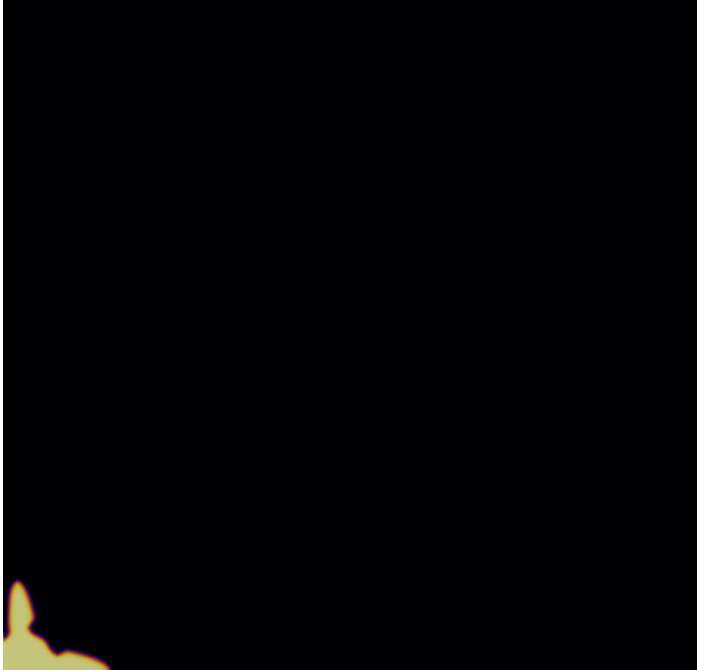
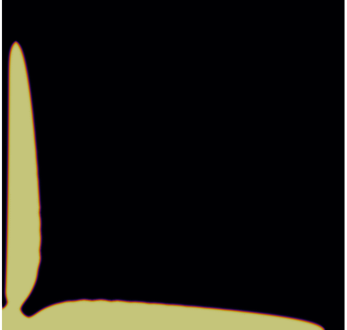
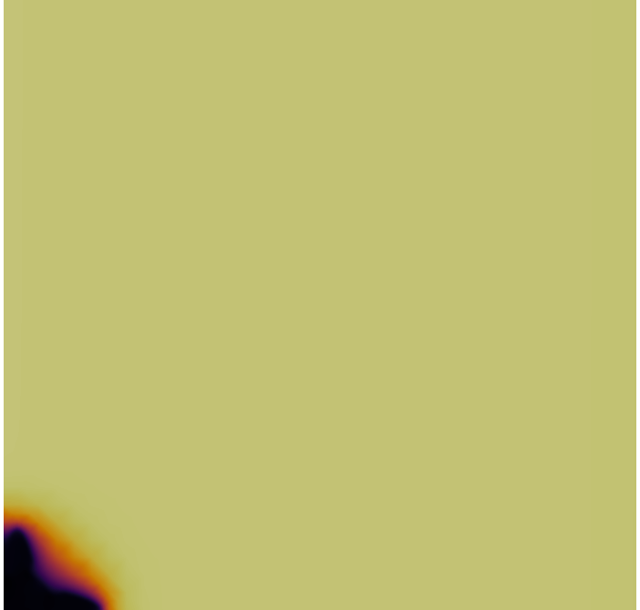
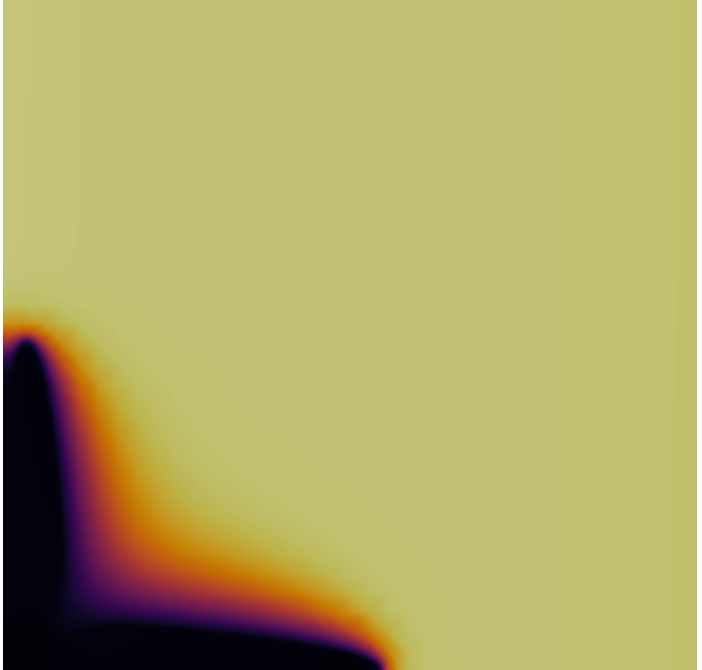
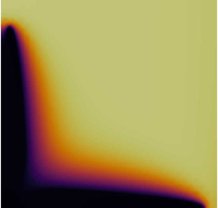
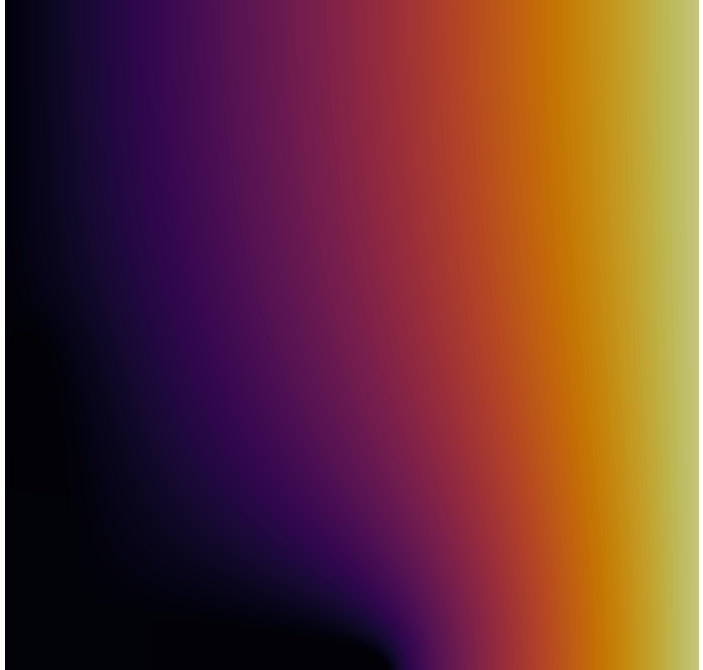
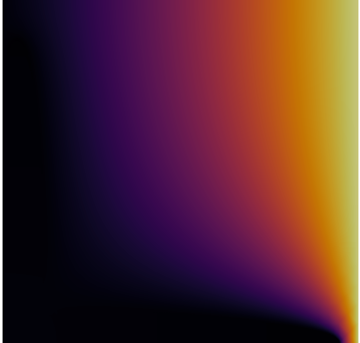
Hình 2. The solution of equations (5.1a)–(5.1c). The order parameter $u$ is at the top row, the concentration $c$ is at the middle row and the electric potential $\phi$ is at the bottom row. The captions are at the times $t_{1}=0.061,t_{2}=0.244$ and $t_{3}=0.427$.

The model we study has a unique solution under certain conditions. One main condition is that the anisotropy strength should always fulfill the inequality $\delta<\delta_{0}=1/(\omega^{2}-1)$. The molecular structure of the lithium atom indicates that $\omega=4$, which represents the mode of the anisotropy. So, $\delta<1/15\approx 0.067$. In Figure 3, the numerical computations show the order parameter for different values of $\delta$. We chose to present several cases for values of $\delta$ that comply with the theoretical limitations for the existence of the weak solution. However, our numerical method treats the anisotropy tensor explicitly and thus we ensure numerical convergence for values that exceed $\delta_{0}$ and so we also present a computation for $\delta=0.1$.

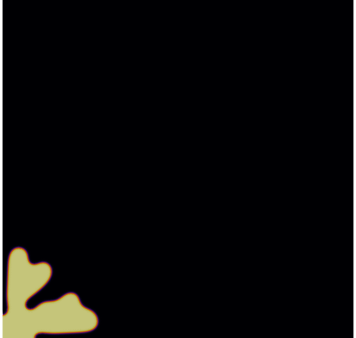
(a) $\delta=0$

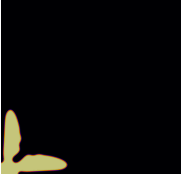
(b) $\delta=0.01$

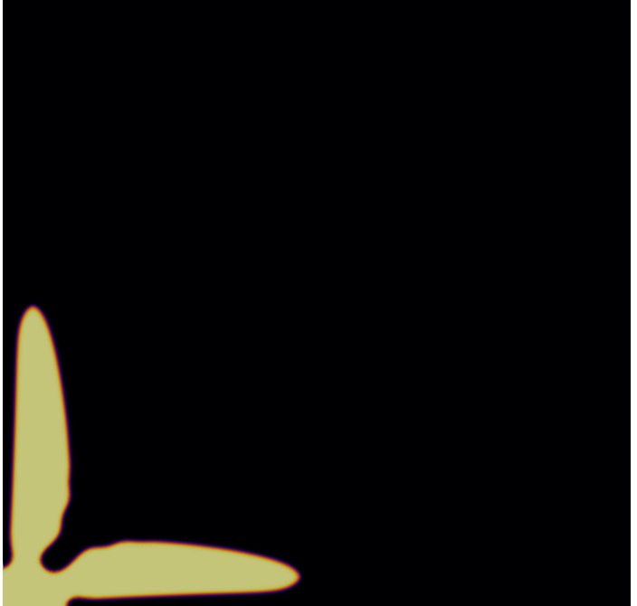
(c) $\delta=0.02$

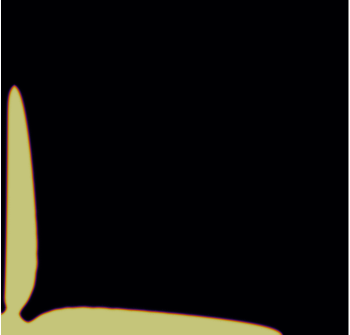
(d) $\delta=0.05$

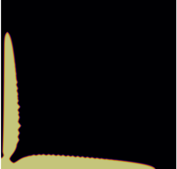
(e) $\delta=0.065$

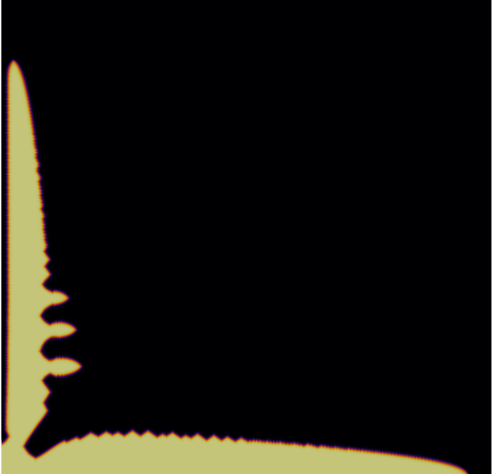
(f) $\delta=0.1$

Hình 3. Comparison of different values for the anisotropy strength $\delta$, which is introduced in (2.29), at $t=0.366$. We observe that image (A) corresponds to the isotropic case of the order parameter. However, the shape is not a sphere because it is affected by the convection–diffusion equation which has as forcing term the time derivative of the order parameter. By increasing the anisotropy strength we see that a crystal shape is formed. Images (B) and (C) show this, but in image (D) we finally see a full crystal shape with only one branch across the x-axis, compared to images (B) and (C), where we see two branches growing across the x-axis. Image (E) represents an experiment for anisotropy strength very close to the theoretical convexity limit $\delta_{0}=1/15$. Image (F) is an example of how the shape is with a value of anisotropy strength that exceeds the theoretical bound for convexivity of the anisotropic Dirichlet energy (2.30).

In Figure 4, we compare how the shaping is affected by the forcing term of the convection–diffusion equation. We have also added an image of a complete isotropic simulation, so that we can compare it with the rest of the results.

(a) isotropic case

(b) $\mu=0$

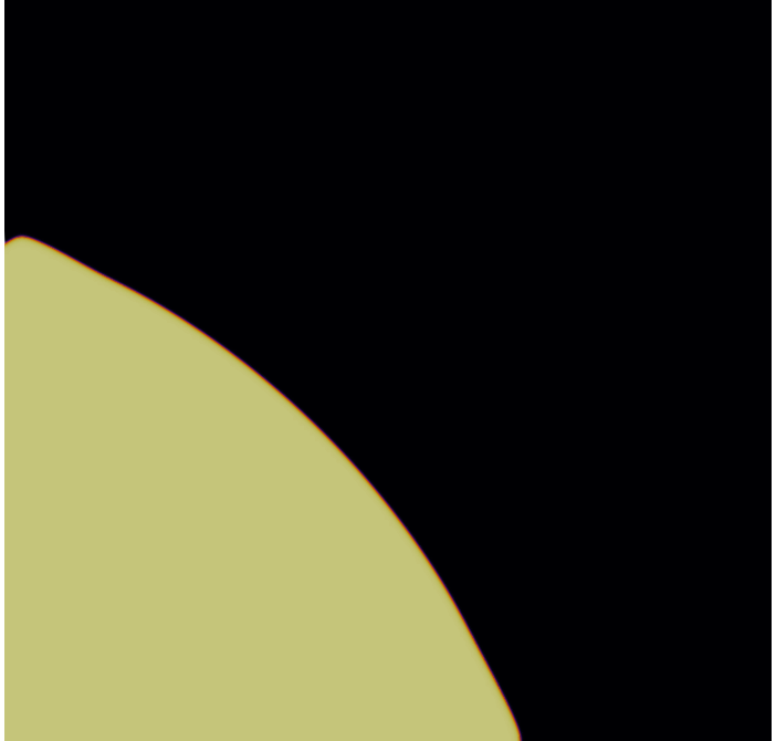
(c) $\mu=0.5$

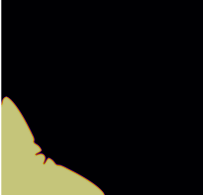
(d) $\mu=1.0$

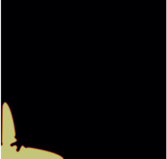
(e) $\mu=1.5$

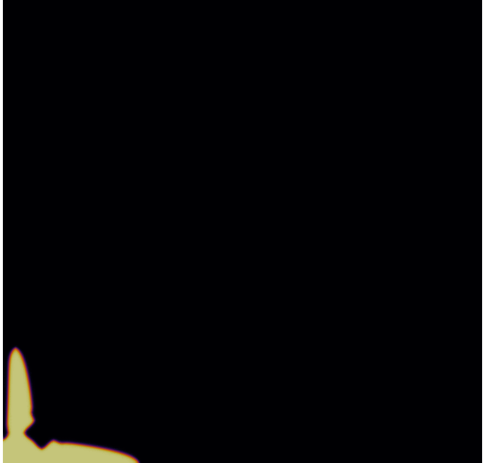
(f) $\mu=2.0$

Hình 4. Comparison of different values for $\mu$ at $t=0.122$. We observe that in the isotropic case we get a sphere. For $\mu=0$ we get an elliptic shape and as we increase the magnitude of the forcing term, as it is formulated in (2.28b), we see that the shape is becoming smaller, but the crystalized structure is more precise.