Multivariate Dynamic Mediation Analysis under a Reinforcement Learning Framework

Abstract

Mediation analysis is an important analytic tool commonly used in a broad range of scientific applications. In this article, we study the problem of mediation analysis when there are multivariate and conditionally dependent mediators, and when the variables are observed over multiple time points. The problem is challenging, because the effect of a mediator involves not only the path from the treatment to this mediator itself at the current time point, but also all possible paths pointed to this mediator from its upstream mediators, as well as the carryover effects from all previous time points. We propose a novel multivariate dynamic mediation analysis approach. Drawing inspiration from the Markov decision process model that is frequently employed in reinforcement learning, we introduce a Markov mediation process paired with a system of time-varying linear structural equation models to formulate the problem. We then formally define the individual mediation effect, built upon the idea of simultaneous interventions and intervention calculus. We next derive the closed-form expression and propose an iterative estimation procedure under the Markov mediation process model. We study both the asymptotic property and the empirical performance of the proposed estimator, and further illustrate our method with a mobile health application.

Key Words: Longitudinal data, Markov process, Mediation analysis, Mobile health, Reinforcement learning

1 Introduction

Mediation analysis is an important analytic tool, which seeks to explain the mechanism or pathway that underlies an observed relationship between a treatment and an outcome variable, through the inclusion of an intermediary variable known as a mediator. It decomposes the effect of the treatment on the outcome into a direct effect and an indirect effect, the latter of which indicates whether the mediator is on a pathway from the treatment to the outcome (Baron and Kenny,, 1986). Mediation analysis is widely employed in a range of scientific applications, including psychology (MacKinnon,, 2008; Rucker et al.,, 2011), genomics (Huang and Pan,, 2016; Bi et al.,, 2017), economics (Celli,, 2022), social science (Kaufman and Kaufman,, 2001), neuroscience (Zhao and Luo,, 2022), among many others. See VanderWeele, (2016) for a comprehensive review and the references therein.

Mediation analysis has seen considerable progress in recent years. There are two lines of research of particular interest, mediation analysis with multivariate mediators, and mediation analysis with time-varying variables.

The first line targets the scenario where there are multiple mediators, and one central goal is to evaluate and quantify the contribution of the treatment on the outcome attributed to each individual mediator. There are three main categories of solutions. One category explicitly imposes that the multivariate mediators are conditionally independent given the treatment, which substantially simplifies the analysis (Boca et al.,, 2014; Huang and Pan,, 2016; Zhang et al.,, 2016; Guo et al.,, 2023; Yuan and Qu,, 2023). Another category does not impose such a condition, but instead marginalizes each individual mediator, which in effect neglects any potential interaction and dependency among the mediators (Sampson et al.,, 2018; Djordjilović et al.,, 2022; Zhao et al.,, 2022; Zhao and Luo,, 2022). The last category does allow correlated mediators, characterizes their dependency through some unknown directed acyclic graph (DAG), then carries out mediation analysis based on the estimated DAG (Maathuis et al.,, 2009; Chakrabortty et al.,, 2018; Cai et al.,, 2022; Shi and Li,, 2022).

The second line targets the scenario where the treatment, mediator and outcome are observed over multiple time points, or stages. There have been some pioneering works along this line (Selig and Preacher,, 2009; Preacher,, 2015; VanderWeele and Tchetgen Tchetgen,, 2017; Huang and Yuan,, 2017; Zheng and van der Laan,, 2017; Zhao et al.,, 2018; Hejazi et al.,, 2020; Cai et al.,, 2022; Díaz et al.,, 2022; Ge et al.,, 2023). Nevertheless, they all focus on the case where there is only a single mediator, and most only consider the case where the number of time points, or the time horizon, is finite.

In this article, we study the problem of mediation analysis when there are multivariate and conditionally dependent mediators, and when the variables are observed over multiple time points in both a finite-horizon setting and an infinite-horizon setting. Our motivation is a mobile health application from the Intern Health Study (IHS, NeCamp et al.,, 2020). It is a 26-week prospective longitudinal randomized trial targeting first-year training physicians in the United States (NeCamp et al.,, 2020). A key objective of this study is to investigate the effectiveness of in-the-moment mobile prompts in improving an intern’s mood score while minimizing user burden and expense. The prompts, delivered through a customized mobile app, consist of practical tips and life insights, such as reminders to have a break, take a walk, or prioritize sleep, that aim at promoting healthy behaviors among interns. These prompts not only affect an intern’s mood, but also influence other physiological measurements, including physical activity, sleep duration, and heart rate variability, which are closely associated with an individual’s mental state. We can naturally formulate this problem in the framework of mediation analysis, where the treatment is the binary variable that encodes receiving or not receiving a prompt, regardless of the prompt type, the mediators consist of measurements of physical activities, sleep duration, and heart rate variability, and the outcome is the mood score. Given the presence of multiple mediators and the longitudinal nature of the data, it calls for a mediation analysis approach that tackles both multivariate mediators and multiple time points.

However, the problem is challenging, for several reasons. First of all, multivariate and conditionally correlated mediators introduce considerable complexity. Unlike the single mediator or conditionally independent mediator case, the indirect effect of each individual mediator involves not only the path from the treatment to this mediator itself, but also all possible paths pointed to this mediator from its upstream mediators. The total number of potential paths that go through any mediator is super-exponential in the number of mediators. It is thus crucial to carefully disentangle the individual mediation effect when the multivariate mediators are interrelated with unknown dependency. Second, time-varying variables introduce another layer of complexity, as there are carryover effects along the time horizon. Unlike the single time point case, the mediator at a given time point could affect both the current and future outcomes, and thus it is crucial to learn both the immediate effect and the delayed effect. Infinite time horizon further complicates the analysis when defining the mediator effect that accumulates over time.

To address those challenges, we propose a novel multivariate dynamic mediation analysis approach. Our proposal consists of four key components. First, drawing inspiration from the Markov decision process (MDP, Puterman,, 2014) model that is frequently employed in reinforcement learning (RL, Sutton and Barto,, 2018) to handle the carryover effects over time, we introduce a Markov mediation process (MMP) framework to formulate the dynamic mediation analysis problem. We then introduce a system of time-varying linear structural equation models (SEMs) to specifically characterize the relations among the treatment, mediator and outcome variables. Second, within the framework of MMP, we formally define the individual mediation effect, which is built upon the idea of simultaneous interventions and intervention calculus (Pearl,, 2000). This individual effect can be further decomposed into a sum of the immediate effect and the delayed effect, the latter of which quantifies the carryover effects of past treatments and mediators. Third, under the proposed MMP and the linear SEMs, we derive the closed-form expression for the individual mediation effect; see Theorems 1 and 2 for details. These theorems form the basis of our estimation procedure, allowing us to express the individual mediation effect using a set of within-stage and cross-stage intermediate quantities that can be estimated through some recursive formulations. We then propose to estimate those within-stage quantities through linear regressions with backdoor covariate adjustment, and estimate those cross-stage quantities through the transition equations under SEMs. Finally, we study the asymptotic property and the empirical performance of our proposed estimator of the individual mediation effect. In summary, our approach allows us to separately evaluate the contribution of each individual mediator, where multiple mediators are interrelated with unknown dependency and are observed over multiple time stages under both finite and infinite-horizon settings.

The rest of the article is organized as follows. We present the Markov mediation process, the structural equation models, and the definition of the individual mediation effect in Section 2. We derive the intermediate quantities, the recursive formulation of the individual mediation effect, and the estimation algorithms in Section 3. We establish the asymptotic properties in Section 3.5. We carry out the simulations in Section 4, and revisit the IHS example in Section 5. We relegate all technical proofs to the Supplementary Material.

2 Model and Definition

In this section, we first present our model assumptions, then formally define the individual mediation effect under the setting of multivariate dynamic mediation analysis.

2.1 Markov mediation process and structural equation models

We first introduce a Markov mediation process framework to formulate the problem we target; see Figure 1 for a graphical illustration. Consider the treatment-mediator-outcome triplets $\left\{\left(A_{t},\bm{M}_{t},R_{t}\right):t=1,\ldots,T\right\}$ over time, where $T$ denotes the number of time points or stages. At each time point or stage $t$, a random treatment $A_{t}\in\mathbb{R}$ is administered, which subsequently affects a $d$-dimensional vector of potential mediators $\bm{M}_{t}\in\mathbb{R}^{d}$, and an outcome variable $R_{t}\in\mathbb{R}$. We assume the data satisfy the Markov assumption, in that

$$(R_{t},\bm{M}_{t})\ \;\,\rule[0.0pt]{0.29999pt}{6.69998pt}\rule[-0.20004pt]{6.99997pt}{0.29999pt}\rule[0.0pt]{0.29999pt}{6.69998pt}\;\,\ (R_{s},\bm{M}_{s},A_{s+1})_{s<t-1}\ \big{|}\ (R_{t-1},\bm{M}_{t-1},A_{t}),\;\text{ for any }t\geq 1,$$ (1)

where         denotes statistical independence. We remark the Markov condition like (1) is widely imposed in sequential data problems. For instance, in reinforcement learning, the state-action-reward triplets are commonly assumed to satisfy the Markov condition (Sutton and Barto,, 2018). In the finite-horizon setting, we allow the process $\{A_{t},\bm{M}_{t},R_{t}\}$ to be non-stationary, whereas in the infinite-horizon setting, we require the process to be stationary over time, which is crucial for consistent learning of the individual mediation effect. Suppose the observed data consists of $n$ independent and identically distributed (i.i.d.) realizations of the triplets $\{(A_{t},\bm{M}_{t},R_{t}):t=1,\ldots,T\}$.

We further assume that the random treatment assignment is independent of the prior information, in that

$$A_{t}\ \;\,\rule[0.0pt]{0.29999pt}{6.69998pt}\rule[-0.20004pt]{6.99997pt}{0.29999pt}\rule[0.0pt]{0.29999pt}{6.69998pt}\;\,\ (A_{s},\bm{M}_{s},R_{s}),\;\text{ for any }s<t.$$ (2)

Condition (2) holds in the sequentially randomized trials naturally, including our IHS example, which is the main setting we target in this article.

We next introduce a system of time-varying structural equation models,

$$(\bm{M}_{t}-\bm{\mu}_{t})=\bm{W}_{t}^{\mbox{\tiny{\sf T}}}(\bm{M}_{t}-\bm{\mu}_{t})+\bm{\epsilon}_{wt},$$ (3)

where $\bm{\mu}_{t}\equiv\mathbb{E}\left(\bm{M}_{t}\mid A_{t},\bm{M}_{t-1},R_{t-1}\right)$ is the condition mean function, $\bm{W}_{t}\in\mathbb{R}^{d\times d}$ is the weight matrix, such that $(\bm{W}_{t})_{ij}\neq 0$ if and only if mediator $M_{ti}$ is a parent of $M_{tj}$, i.e., $M_{ti}$ is in the parent set, $M_{ti}\in\mathrm{Pa}(M_{tj})\equiv\big{\{}M_{ti}:(\bm{W}_{t})_{ij}\neq 0,i\in\{1,\ldots,d\}\setminus\{j\}\big{\}}$, and $\bm{\epsilon}_{wt}=(\epsilon_{w,1t},\ldots,\epsilon_{w,dt})^{\mbox{\tiny{\sf T}}}\in\mathbb{R}^{d}$ is a vector of mean zero random errors. In model (3), the weight matrix $\bm{W}_{t}$ models the interactions among the mediators $\bm{M}_{t}$ at each time point, and the conditional mean $\bm{\mu}_{t}$ characterizes the dynamic dependence over time.

We then consider linear models for $\bm{\mu}_{t}$ and $R_{t}$, in that

$$\begin{split}\bm{\mu}_{t}&=\bm{\alpha}_{1t}+\bm{\delta}_{1t}A_{t}+\bm{\Gamma}_{1t}\bm{M}_{t-1}+\bm{\zeta}_{1t}R_{t-1},\\ R_{t}&=\alpha_{2t}+\delta_{2t}A_{t}+\bm{\gamma}_{2t}^{\mbox{\tiny{\sf T}}}\bm{M}_{t-1}+\zeta_{2t}R_{t-1}+\bm{\kappa}_{t}^{\mbox{\tiny{\sf T}}}\bm{M}_{t}+\epsilon_{rt},\end{split}$$ (4)

for some $\bm{\alpha}_{1t},\bm{\delta}_{1t},\bm{\zeta}_{1t}\in\mathbb{R}^{d}$ and $\bm{\Gamma}_{1t}\in\mathbb{R}^{d\times d}$, and for some $\bm{\gamma}_{2t},\bm{\kappa}_{t}\in\mathbb{R}^{d}$, $\alpha_{2t},\delta_{2t},\zeta_{2t}\in\mathbb{R}$ and some mean zero errors $\{\epsilon_{rt}\}_{t}$ independent over time, respectively. Let $\bm{\Theta}_{1t}\equiv(\bm{\alpha}_{1t},\bm{\delta}_{1t},\bm{\Gamma}_{1t},\bm{\zeta}_{1t})\in\mathbb{R}^{d\times(d+3)}$ collect all the parameters for $\bm{\mu}_{t}$ in (4), and $\bm{\Theta}_{2t}\equiv(\alpha_{2t},\delta_{2t},\bm{\gamma}_{2t}^{\mbox{\tiny{\sf T}}}$, $\zeta_{2t},\bm{\kappa}_{t}^{\mbox{\tiny{\sf T}}})^{\mbox{\tiny{\sf T}}}\in\mathbb{R}^{(2d+3)\times 1}$ collect all the parameters for $R_{t}$ in (4).

We make a few remarks. First, we draw a connection between the proposed MMP and MDP commonly studied in reinforcement learning, a powerful machine learning technique for optimal sequential decision making (Murphy,, 2003; Mnih et al.,, 2015; Silver et al.,, 2017; Chen et al.,, 2021; Qin et al.,, 2021; Chen et al.,, 2022). Both capture the carryover effects over time. MDP achieves this by introducing a sequence of time-varying feature variables, referred to as the states. It then models the carryover effects through state transitions, allowing past treatments to affect future outcomes through their impact on future states; see Figure 1(a) for an illustration. This approach has gained substantial attention for policy evaluation, serving to model both immediate and long-term effects of a target policy (Luckett et al.,, 2020; Hao et al.,, 2021; Liao et al.,, 2021; Kallus and Uehara,, 2022; Hu and Wager,, 2022; Liao et al.,, 2022; Ramprasad et al.,, 2022; Shi et al.,, 2022; Wang et al.,, 2023). In a similar vein, our MMP operates by modeling the indirect influence of a preceding mediator via the transitions of mediator-outcome pairs. In essence, a past mediator influences future outcomes by exerting its effects on both the prior outcome and the subsequent mediator; see Figure 1(b) for an illustration. Second, the relation in (3) should be understood as a data generating mechanism, rather than as a mere association. It corresponds to a directed acyclic graph (DAG). Third, to keep the presentation simple, we do not include any observed confounders, which may be incorporated into our solution in a relatively straightforward fashion. We do not consider any unobserved confounders either, because we consider random treatment assignments. We leave the case with unobserved confounders as future research. Finally, we consider linear type models in both (3) and (4). The analysis of mediation has been dominated by linear regression paradigms and such linearity assumption is commonly adopted in existing work, see for example, Nandy et al., (2017); Chakrabortty et al., (2018); Shi and Li, (2022). It is possible to extend to nonlinear type models, under which the definition of individual mediation effect we give later still holds, but is more difficult to evaluate.

In summary, we believe that our model framework provides a reasonable starting point for multivariate dynamic mediation analysis. The methodology under our setting is already complex enough, and deserves a careful investigation.

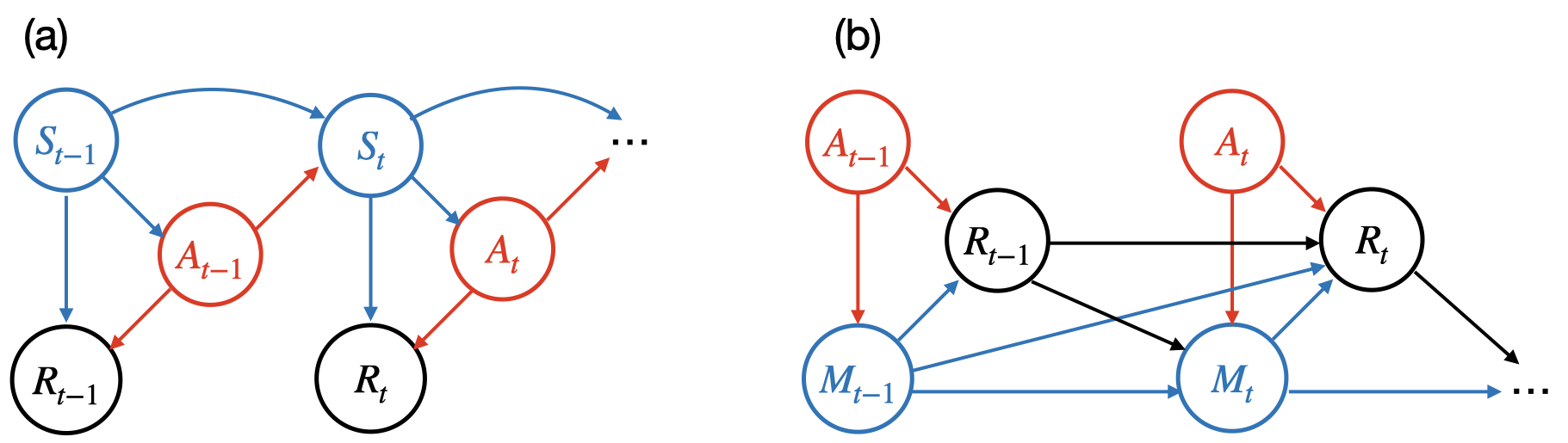
Figure 1: (a) Diagram of MDP where treatments depend on current states only. $(S_{t},A_{t},R_{t})$ denotes the state-treatment-reward triplet; (b) graphical representation of our MMP where current mediators depend on previous mediator-reward pairs. $(A_{t},M_{t},R_{t})$ represents the treatment-mediator-outcome triplet.

2.2 Individual mediation effect

We now formally define the individual mediation effect in our setting. Specifically, we define the individual mediation effect of the $j$th mediator at time point $t$ to be the portion of the total effect of a sequence of treatment variables $\{A_{s}:s\leq t\}$ on the outcome $R_{t}$ that go through $\{M_{sj}:s\leq t\}$, where $M_{sj}$ is the $j$th mediator at time $s$, $1\leq j\leq d$, $1\leq t\leq T$. To quantify those effects, we consider a hypothetical intervention applied to the system, where we set all treatments to some value $a$ uniformly over the entire population. This can be realized through Pearl’s do-operator, $do(A_{t}=a)$, which generates an interventional distribution by removing the edges leading into $\{A_{s}:s\leq t\}$ in the corresponding DAG (Pearl,, 2000). We denote the post-interventional expectation of $R_{t}$ by $\mathbb{E}[R_{t}\mid do(A_{s}=a,\forall s\leq t)]$. Similarly, we also consider the joint-intervention on $(A_{s},M_{sj})$ through $do(A_{s}=a,M_{sj}=m)$, and we denote the post-interventional expectation of $R_{t}$ by $\mathbb{E}[R_{t}\mid do(A_{s}=a,M_{sj}=m,\forall s\leq t)]$. The next two definitions define the individual mediation effect in the finite and infinite-horizon settings, respectively.

Definition 1 (Finite-horizon).

In a finite-horizon setting, the individual mediation effect of the $j$th mediator over $T$ time points or stages is defined as

$$\eta_{j}^{(T)}\equiv\frac{1}{T}\sum_{t=1}^{T}\frac{\partial}{\partial a}\mathbb{E}[R_{t}\mid do(A_{s}=a,\forall s\leq t)]-\frac{1}{T}\sum_{t=1}^{T}\frac{\partial}{\partial a}\mathbb{E}[R_{t}\mid do(A_{s}=a,M_{sj}=m,\forall s\leq t)].$$

Definition 2 (Infinite-horizon).

In an infinite-horizon setting, the individual mediation effect of the $j$th mediator is defined as $\eta_{j}^{(\infty)}\equiv\underset{T\to\infty}{\lim}\eta_{j}^{(T)}$, provided that the limit exists.

We make a few remarks. First, the term $\partial\mathbb{E}[R_{t}\mid do(A_{s}=a,\forall s\leq t)]/\partial a$ in Definition 1 measures the total effect of treatments $\{A_{s}\}_{s\leq t}$ on $R_{t}$, whereas the term $\partial\mathbb{E}[R_{t}\mid do(A_{s}=a,M_{sj}=m,\forall s\leq t)]/\partial a$ corresponds to the total effect of $\{A_{s}\}_{s\leq t}$ on $R_{t}$ when setting the interventional values of $\{M_{1j},\dots,M_{tj}\}$ to a constant. When the treatment takes a discrete value, the derivative in those terms can be substituted by the difference operator. For instance, if the treatment is binary, we obtain the following formula,

$$\eta_{j}^{(T)}=\sum_{a=0}^{1}(-1)^{a+1}\frac{1}{T}\bigg{\{}\sum_{t=1}^{T}\mathbb{E}[R_{t} \mid do(A_{s}=a,\forall s\leq t)]$$

$$-\sum_{t=1}^{T}\mathbb{E}[R_{t}\mid do(A_{s}=a,M_{sj}=m,\forall s\leq t)]\bigg{\}}.$$

Second, the definition of the individual mediation effect does not require linear structural equation models like (4). However, imposing such models greatly simplify the analysis. More specifically, in a general Markov mediation process, $\eta_{j}^{(T)}$ can depend on $(a,m)$ in a very complex manner, whereas (4) simplifies $\eta_{j}^{(T)}$ as a constant function of $(a,m)$; see Section 3 for more details. In addition, we observe that, under (4), the second post-interventional expectation term, $\mathbb{E}[R_{t}\mid do(A_{s}=a,M_{sj}=m,\forall s\leq t)]$, may be analyzed by the path method (Wright,, 1921). That is, it can be calculated by summing up the effects along all directed paths from $\{A_{s}\}_{s\leq t}$ to $R_{t}$ that do not pass through $\{M_{sj}\}_{s\leq t}$. However, this approach can be computationally expensive, since the number of paths grows exponentially fast as the number of time points $T$ increases.

Finally, Definitions 1 and 2 are concerned with the cumulative mediation effect over time. Alternatively, one may be interested in the incremental effect, i.e.,

$$\Delta_{j}^{(t)}\equiv\frac{\partial}{\partial a}\mathbb{E}[R_{t}\mid do(A_{s}=a,\forall s\leq t)]-\frac{\partial}{\partial a}\mathbb{E}[R_{t}\mid do(A_{s}=a,M_{sj}=m,\forall s\leq t)],$$

which can be interpreted as the change in the total effect of the sequence of treatments $\{A_{s}\}_{s\leq t}$ on the outcome $R_{t}$ when the $j$th mediator is intervened by $do(M_{sj}=m,\forall s\leq t)$. By definition, it is immediate to see that this incremental effect is related to the cumulative effect, in that $\eta_{j}^{(T)}=T^{-1}\sum_{t=1}^{T}\Delta_{j}^{(t)}$. Moreover, to better understand our definition of individual mediation effect, we further decompose $\Delta_{j}^{(t)}$ into the sum of the immediate individual mediation effect (IIME) and the delayed individual mediation effect (DIME), which are defined as follows.

Definition 3.

Define the immediate individual mediation effect (IIME) and the delayed individual mediation effect (DIME) as,

$$\mathrm{IIME}_{j}^{(t)} \equiv \frac{\partial}{\partial a}\mathbb{E}[R_{t}\mid do(A_{t}=a)]-\frac{\partial}{\partial a}\mathbb{E}[R_{t}\mid do(A_{t}=a,M_{tj}=m)],$$

$$\mathrm{DIME}_{j}^{(t)} \equiv \Delta_{j}^{(t)}-\mathrm{IIME}_{j}^{(t)}.$$

At a given time point $t$, $\text{IIME}_{j}^{(t)}$ can be interpreted as the change in the total effect of $A_{t}$ on $R_{t}$ when $M_{tj}$ is knocked out, whereas $\text{DIME}_{j}^{(t)}$ captures the individual mediation effect of the $j$th mediator that is carried over from all previous stages $s<t$ up to time $t$.

We comment that all above definitions seem natural and agree with the intuitions. We next discuss how to evaluate and estimate the individual mediation effect.

3 Evaluation of Individual Mediation Effect

In this section, we propose an approach to evaluate the individual mediation effect given in Definitions 1 and 2. The problem, however, is very challenging, as we have to deal with both the multiple mediators with unknown correlation structure, as well as the carryover effects from the upstream treatments and mediators. Our proposed solution involves deriving a closed-form expression for the individual mediation effect, detailed in Theorems 1 and 2. This expression is dependent on several intermediate quantities that are computable through a set of recursive relations. Leveraging these theoretical findings, we have developed an efficient recursive computation algorithm to estimate these intermediate quantities, subsequently facilitating the estimation of the individual mediation effect.

3.1 An illustrative example

To illustrate our theory, we first consider a simple example as shown in Figure 2, in which there are only $d=2$ mediators and $T=2$ time stages. We then extend our observations to more general cases with $d$ mediators and $T$ stages.

Suppose we focus on the individual mediation effect for the second mediator, i.e., $j=2$. We begin with the first stage $t=1$, as shown in Figure 2, left panel. By Definition 1,

$$\eta_{2}^{(1)}=\frac{\partial}{\partial a}\mathbb{E}[R_{1}\mid do(A_{1}=a)]-\frac{\partial}{\partial a}\mathbb{E}[R_{1}\mid do(A_{1}=a,M_{12}=m)]\equiv\theta_{A_{1}\to R_{1}}-\theta_{A_{1}\to R_{1}}^{M_{12}},$$ (5)

where we use the notation $\theta_{A_{1}\to R_{1}}$ to denote the total effect from $A_{1}$ to $R_{1}$, and use $\theta_{A_{1}\to R_{1}}^{M_{12}}$ to denote the total effect from $A_{1}$ to $R_{1}$ when the second mediator is intervened in the first stage.

We compute $\theta_{A_{1}\to R_{1}}$ by summing up the effects along all directed paths from $A_{1}$ to $R_{1}$, namely, $A_{1}\to R_{1}$, $A_{1}\to M_{11}\to R_{1}$, $A_{1}\to M_{12}\to R_{1}$, and $A_{1}\to M_{11}\to M_{12}\to R_{1}$. Meanwhile, we compute $\theta_{A_{1}\to R_{1}}^{M_{12}}$ by eliminating all paths that go from $A_{1}$ to $R_{1}$ through $M_{12}$. This corresponds to subtracting the effects along $A_{1}\to M_{12}\to R_{1}$ and $A_{1}\to M_{11}\to M_{12}\to R_{1}$, which leads to

$$\theta_{A_{1}\to R_{1}}^{M_{12}}=\theta_{A_{1}\to R_{1}}-\theta_{A_{1}\to M_{12}}\theta_{M_{12}\to R_{1}},$$ (6)

where we use the notation $\theta_{A_{1}\to M_{12}}$ and $\theta_{M_{12}\to R_{1}}$ to denote the effect from $A_{1}$ to $M_{12}$, and from $M_{12}$ to $R_{1}$, respectively. The relation in (6) has an intuitive interpretation: to evaluate the total effect from $A_{1}$ to $R_{1}$ when $M_{12}$ is intervened, we subtract from $\theta_{A_{1}\to R_{1}}$ the effects along the subset of paths that go through $M_{12}$. Plugging (6) into (5), we obtain that $\eta_{2}^{(1)}=\theta_{A_{1}\to M_{12}}\theta_{M_{12}\to R_{1}}$, which coincides with the classical product type representation of the individual mediation effect in a single-stage analysis (Nandy et al.,, 2017).

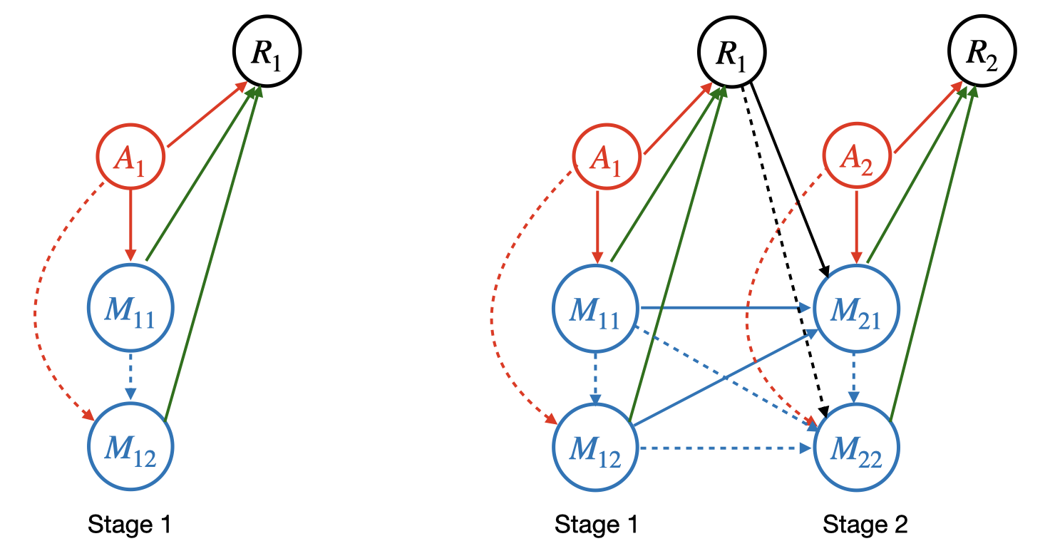
Figure 2: An illustrative example with two mediators and two time stages. The left panel shows the DAG in the first stage, and the right panel the first two stages. The dashed lines highlight the paths that go through the intervened mediator, i.e., the second mediator.

We next move to the second stage $t=2$, as in Figure 2, right panel. By Definition 1,

$$\eta_{2}^{(2)} =\frac{1}{2}\eta_{2}^{(1)}+\frac{1}{2}\bigg{\{}\frac{\partial}{\partial a}\mathbb{E}[R_{2}\mid do(A_{1}=A_{2}=a)]$$ (7)

$$-\frac{\partial}{\partial a}\mathbb{E}[R_{2}\mid do(A_{1}=A_{2}=a,M_{12}=M_{22}=m)]\bigg{\}}\equiv\frac{1}{2}\eta_{2}^{(1)}+\frac{1}{2}\left(\theta_{A_{1},A_{2}\to R_{2}}-\theta_{A_{1},A_{2}\to R_{2}}^{M_{12},M_{22}}\right),$$

where we use the notation $\theta_{A_{1},A_{2}\to R_{2}}$ to denote the cumulative total effect of $(A_{1},A_{2})$ on $R_{2}$, and use $\theta_{A_{1},A_{2}\to R_{2}}^{M_{12},M_{22}}$ to denote the cumulative total effect of $(A_{1},A_{2})$ on $R_{2}$ when the second mediator is intervened in both the first and second stages.

Because the treatments are randomly assigned and their parent sets are empty, we have,

$$\theta_{A_{1},A_{2}\to R_{2}}=\theta_{A_{1}\to R_{2}}+\theta_{A_{2}\to R_{2}},\quad\quad\theta_{A_{1},A_{2}\to R_{2}}^{M_{12},M_{22}}=\theta_{A_{1}\to R_{2}}^{M_{12},M_{22}}+\theta_{A_{2}\to R_{2}}^{M_{22}},$$ (8)

where we use the notation $\theta_{A_{1}\to R_{2}}$ and $\theta_{A_{2}\to R_{2}}$ to denote the total effects from $A_{1}$ to $R_{2}$, and from $A_{2}$ to $R_{2}$, respectively, use $\theta_{A_{2}\to R_{2}}^{M_{22}}$ to denote the effect from $A_{2}$ to $R_{2}$ when the second mediator is intervened in the second stage, and use $\theta_{A_{1}\to R_{2}}^{M_{12},M_{22}}$ to denote the effect from $A_{1}$ to $R_{2}$ when the second mediator is intervened in both stages.

We compute $\theta_{A_{1}\to R_{2}}$ and $\theta_{A_{2}\to R_{2}}$ similarly as that for $\theta_{A_{1}\to R_{1}}$. We compute $\theta_{A_{2}\to R_{2}}^{M_{22}}$ similarly as in (6), i.e., $\theta_{A_{2}\to R_{2}}^{M_{22}}=\theta_{A_{2}\to R_{2}}-\theta_{A_{2}\to M_{22}}\theta_{M_{22}\to R_{2}}$. Also, similar to (6), we have,

$$\theta_{A_{1}\to R_{2}}^{M_{12},M_{22}}=\theta_{A_{1}\to R_{2}}^{M_{22}}-\theta_{A_{1}\to M_{12}}\theta_{M_{12}\to R_{2}}^{M_{22}},$$ (9)

where we use $\theta_{A_{1}\to R_{2}}^{M_{22}}$ and $\theta_{M_{12}\to R_{2}}^{M_{22}}$ to denote the effects from $A_{1}$ to $R_{2}$, and from $M_{12}$ to $R_{2}$, when the second mediator is intervened in the second stage. Intuitively, $\theta_{M_{12}\to R_{2}}^{M_{22}}$ can be interpreted as the carryover effect of the second mediator on the outcome from the first stage to the second stage when it is intervened. We again compute $\theta_{A_{1}\to R_{2}}^{M_{22}}$ similarly to (6), i.e., $\theta_{A_{1}\to R_{2}}^{M_{22}}=\theta_{A_{1}\to R_{2}}-\theta_{A_{1}\to M_{22}}\theta_{M_{22}\to R_{2}}$. In addition, we compute $\theta_{M_{12}\to R_{2}}^{M_{22}}$ by eliminating all paths that go from $M_{12}$ to $R_{2}$ through $M_{22}$, which leads to

$$\theta_{M_{12}\to R_{2}}^{M_{22}}=\theta_{M_{12}\to R_{2}}-\theta_{M_{12}\to M_{22}}\theta_{M_{22}\to R_{2}},$$ (10)

where we use $\theta_{M_{12}\to R_{2}}$, $\theta_{M_{12}\to M_{22}}$, and $\theta_{M_{22}\to R_{2}}$ to denote the effects from $M_{12}$ to $R_{2}$, from $M_{12}$ to $M_{22}$, and from $M_{22}$ to $R_{2}$, respectively.

Based on the derivations so far, we see that, to evaluate the individual mediation effect, it is crucial to calculate those intermediate quantities, such as $\theta_{A_{1}\to R_{1}},\theta_{A_{1}\to M_{22}},\theta_{M_{12}\to M_{22}}$, $\theta_{M_{22}\to R_{2}}$, among others. Next, we briefly discuss how to evaluate those intermediate quantities after imposing the linear structural equation models (3) and (4). We also discuss some recursive relation that facilitates both the computational and statistical efficiency.

First, we note that, under (3) and (4), we can estimate those intermediate quantities through linear regressions. For instance, we can estimate $\theta_{A_{1}\to R_{1}}$ as the coefficient of $A_{1}$ by linearly regressing $R_{1}$ onto $A_{1}$. Meanwhile, we can estimate $\theta_{M_{22}\to R_{2}}$ as the coefficient of $M_{22}$ by linearly regressing $R_{2}$ onto $M_{22}$, however, with some additional covariate adjustment. This is because, unless the two mediators $(M_{21},M_{22})$ are conditionally independent given $(M_{11},M_{12},R_{1},A_{2})$, we need to adjust for a set of covariates that satisfy Pearl’s backdoor criterion (Pearl,, 2000). In other words, we should block the effects flowing from $(A_{2},M_{11},M_{12},M_{21},R_{1})$ to $M_{22}$. Therefore, we need to adjust for the covariate set $\mathrm{Pa}(M_{22})\cup{M_{11}}\cup M_{12}\cup R_{1}\cup A_{2}$ in this regression.

Second, we note that, the set of intermediate quantities involve both within-stage quantities such as $\theta_{A_{1}\to R_{1}},\theta_{M_{22}\to R_{2}}$, as well as cross-stage quantities such as $\theta_{A_{1}\to M_{22}},\theta_{M_{12}\to M_{22}}$. There is some useful recursive relation between the within-stage and cross-stage quantities under the linear structural equation models (3) and (4). For instance,

$$\bm{\theta}_{A_{1}\to\bm{M}_{2}}=\bm{\Gamma}_{12}\bm{\theta}_{A_{1}\to\bm{M}_{1}}+\bm{\zeta}_{12}\theta_{A_{1}\to R_{1}},$$ (11)

where $\bm{\theta}_{A_{1}\to\bm{M}_{2}}=(\theta_{A_{1}\to M_{21}},\theta_{A_{1}\to M_{22}})^{\mbox{\tiny{\sf T}}}$, and $\bm{\theta}_{A_{1}\to\bm{M}_{1}}=(\theta_{A_{1}\to M_{11}},\theta_{A_{1}\to M_{12}})^{\mbox{\tiny{\sf T}}}$. This suggests that the cross-stage carryover effect from $A_{1}$ to $\bm{M}_{2}=(M_{21},M_{22})^{\mbox{\tiny{\sf T}}}$ is a combination of its within-stage effect on $\bm{M}_{1}=(M_{11},M_{12})^{\mbox{\tiny{\sf T}}}$ and on $R_{1}$, respectively, whereas the coefficients $(\bm{\Gamma}_{12},\bm{\zeta}_{12})$ can be viewed as the weights or discount factors for such a cross-stage transition. In our estimation algorithm, we first estimate the within-stage quantities via linear regressions, then update the cross-stage quantities following (11). As we show later, the relation such as (11) not only expedites the computation, but also improves the estimation efficiency by leveraging more information from the conditional model (4).

In summary, this simple example reveals a number of important relations. First, we see that those intermediate quantities form the building blocks for our evaluation of the individual mediation effect. Second, (6), (9), and (10) suggest some useful recursive representations that in effect reduce the number of mediators in the superscript that are intervened upon. Third, under models (3) and (4), we can estimate those intermediate quantities through linear regressions, with possibly backdoor adjustment. Finally, we can further improve both the computational and statistical efficiency through another set of recursive relations between the within-stage and cross-stage quantities. All these observations are crucial for our derivation of the expression for the individual mediation effect.

3.2 Intermediate quantities

We now formally define the set of all intermediate quantities that are needed for the evaluation of the individual mediation effect. We then discuss how to estimate those quantities.

For any $1\leq s\leq t\leq T$, and $j=1,\ldots,d$, define

$$\begin{split}&\theta_{A_{s}\to R_{t}}\equiv\frac{\partial}{\partial a}\mathbb{E}[R_{t}\mid do(A_{s}=a)]\in\mathbb{R},\quad\,\ \bm{\theta}_{M_{sj}\to\bm{M}_{t}}\equiv\frac{\partial}{\partial m}\mathbb{E}[\bm{M}_{t}\mid do(M_{sj}=m)]\in\mathbb{R}^{d},\\ &\bm{\theta}_{A_{s}\to\bm{M}_{t}}\equiv\frac{\partial}{\partial a}\mathbb{E}[\bm{M}_{t}\mid do(A_{s}=a)]\in\mathbb{R}^{d},\;\theta_{M_{sj}\to R_{t}}\equiv\frac{\partial}{\partial m}\mathbb{E}[R_{t}\mid do(M_{sj}=m)]\in\mathbb{R}.\end{split}$$ (12)

These intermediate quantities in (12) can be obtained through linear regressions, either directly, or by some backdoor covariate adjustment. In particular, $\theta_{A_{s}\to R_{t}}$ can be obtained as the coefficient of $A_{s}$ by linearly regressing $R_{t}$ onto $A_{s}$ with an intercept, and we write this coefficient as $\beta_{A_{s},R_{t}}$. Similarly, $\bm{\theta}_{A_{s}\to\bm{M}_{t}}$ can be obtained as the coefficient of $A_{s}$ by linearly regressing $\bm{M}_{t}$ onto $A_{s}$, denoted as $\bm{\beta}_{A_{s},\bm{M}_{t}}$. Meanwhile, $\theta_{M_{sj}\to R_{t}}$ can be obtained as the coefficient of $M_{sj}$ by linearly regressing $R_{t}$ onto $M_{sj}$, along with the adjusted covariate set, $\mathrm{Pa}(M_{sj})\cup{\bm{M}_{s-1}}\cup R_{s-1}\cup A_{s}$. Similarly, $\theta_{M_{sj}\to\bm{M}_{t}}$ can be obtained as the coefficient of $M_{sj}$ by linearly regressing $\bm{M}_{t}$ onto $M_{sj}$, along with the adjusted covariate set, $\mathrm{Pa}(M_{sj})\cup{\bm{M}_{s-1}}\cup R_{s-1}\cup A_{s}$. Putting together, we have,

$$\begin{split}&\theta_{A_{s}\to R_{t}}=\beta_{A_{s},R_{t}},\quad\quad\bm{\theta}_{M_{sj}\to\bm{M}_{t}}=\bm{\beta}_{M_{sj},\bm{M}_{t}\mid\mathrm{Pa}(M_{sj})\cup{\bm{M}_{s-1}}\cup R_{s-1}\cup A_{s}},\\ &\bm{\theta}_{A_{s}\to\bm{M}_{t}}=\bm{\beta}_{A_{s},\bm{M}_{t}},\quad\,\theta_{M_{sj}\to R_{t}}=\beta_{M_{sj},R_{t}\mid\mathrm{Pa}(M_{sj})\cup\bm{M}_{s-1}\cup R_{s-1}\cup A_{s}}.\end{split}$$ (13)

Moreover, similar to (11), we obtain the following recursive relations between the within-stage quantities and the cross-stage quantities. That is, under models (3) and (4),

$$\begin{split}&\theta_{A_{s}\to R_{t}}=\zeta_{2t}\theta_{A_{s}\to R_{t-1}}+\bm{\kappa}_{t}^{\mbox{\tiny{\sf T}}}\bm{\theta}_{A_{s}\to\bm{M}_{t}}+\bm{\gamma}_{2t}^{\mbox{\tiny{\sf T}}}\bm{\theta}_{A_{s}\to\bm{M}_{t-1}},\\ &\bm{\theta}_{A_{s}\to\bm{M}_{t}}=\bm{\Gamma}_{1t}\bm{\theta}_{A_{s}\to\bm{M}_{t-1}}+\bm{\zeta}_{1t}\theta_{A_{s}\to R_{t-1}},\\ &\theta_{M_{sj}\to R_{t}}=\zeta_{2t}\theta_{M_{sj}\to R_{t-1}}+\bm{\kappa}_{t}^{\mbox{\tiny{\sf T}}}\bm{\theta}_{M_{sj}\to\bm{M}_{t}}+\bm{\gamma}_{2t}^{\mbox{\tiny{\sf T}}}\bm{\theta}_{M_{sj}\to\bm{M}_{t-1}},\\ &\bm{\theta}_{M_{sj}\to\bm{M}_{t}}=\bm{\Gamma}_{1t}\bm{\theta}_{M_{sj}\to\bm{M}_{t-1}}+\bm{\zeta}_{1t}\theta_{M_{sj}\to R_{t-1}}.\end{split}$$ (14)

In our implementation, we first estimate the within-stage quantities, $\{\theta_{A_{t}\to R_{t}},\theta_{M_{tj}\to R_{t}}$, $\bm{\theta}_{A_{t}\to\bm{M}_{t}},\bm{\theta}_{M_{tj}\to\bm{M}_{t}}\}$, using (13), then estimate the cross-stage quantities, $\{\theta_{A_{s}\to R_{t}},\theta_{M_{sj}\to R_{t}}$, $\bm{\theta}_{A_{s}\to R_{t}},\bm{\theta}_{M_{sj}\to\bm{M}_{t}}\}$, for $s=1,\ldots,t-1$, using (14). This helps to improve both the estimation efficiency and the computation efficiency.

3.3 Individual mediation effect in a finite-horizon setting

We next derive the expression of the individual mediation effect through the intermediate quantities in (12) under the finite-horizon setting.

We sketch the key ideas of the derivation here, and relegate a more detailed derivation to the Appendix. By Definition 1, the individual mediation effect of the $j$th mediator across $t$ stages, $j=1,\ldots,d$, $t=1,\ldots,T$, can be expressed as

$$\eta_{j}^{(t)}=\frac{1}{t}\left\{(t-1)\eta_{j}^{(t)}+\theta_{A_{1},\dots,A_{t}\to R_{t}}-\theta_{A_{1},\dots,A_{t}\to R_{t}}^{M_{1j},\dots,M_{tj}}\right\}$$ (15)

Because all the treatments $(A_{1},\ldots,A_{t})$ are randomly assigned, and thus are independent of each other and all other covariates, similar to (8), we have,

$$\begin{split}\theta_{A_{1},\dots,A_{t}\to R_{t}}&=\theta_{A_{1}\to R_{t}}+\theta_{A_{2}\to R_{t}}+\dots+\theta_{A_{t}\to R_{t}},\\ \theta_{A_{1},\dots,A_{t}\to R_{t}}^{M_{1j},\dots,M_{tj}}&=\theta_{A_{1}\to R_{t}}^{M_{1j},\dots,M_{tj}}+\theta_{A_{2}\to R_{t}}^{M_{2j},\dots,M_{tj}}+\dots+\theta_{A_{t}\to R_{t}}^{M_{tj}}.\end{split}$$ (16)

Then, similar to (6), (9), and (10), we obtain the following recursive relations that help reduce the number of mediators being intervened upon. That is, for any $s=1,\ldots,t-1$,

$$\theta_{A_{s}\to R_{t}}^{M_{sj},\ldots,M_{tj}} =\theta_{A_{s}\to R_{t}}^{M_{(s+1)j},\ldots,M_{tj}}-\theta_{A_{s}\to M_{sj}}\theta_{M_{sj}\to R_{t}}^{M_{sj},\ldots,M_{tj}}=\cdots$$

$$=\theta_{A_{s}\to R_{t}}-\sum_{i=s}^{t}\theta_{A_{s}\to M_{ij}}\theta_{M_{ij}\to R_{t}}^{M_{ij},\ldots,M_{tj}};$$ (17)

$$\theta_{M_{sj}\to R_{t}}^{M_{sj},\ldots,M_{tj}} =\theta_{M_{sj}\to R_{t}}^{M_{(s+2)j},\ldots,M_{tj}}-\theta_{M_{sj}\to M_{(s+1)j}}\theta_{M_{(s+1)j}\to R_{t}}^{M_{(s+1)j},\ldots,M_{tj}}=\cdots$$

$$=\theta_{M_{sj}\to R_{t}}-\sum_{i=s+1}^{t}\theta_{M_{sj}\to M_{ij}}\theta_{M_{ij}\to R_{t}}^{M_{ij},\ldots,M_{tj}}.$$ (18)

Combining (15), (16), (17), and (18), we obtain the following theorem with respect to the identification of individual mediation effect in finite-horizon settings. We relegate a more detailed derivation to the Supplementary Appendix.

Theorem 1 (Individual mediation effect for finite-horizon).

Suppose $\{A_{t}\}_{t\geq 1}$ are randomly assigned treatments and satisfy (2), and $\{\bm{M}_{t},R_{t}\}_{t\geq 1}$ follow (3) and (4). Then,

$$\begin{split}\eta_{j}^{(t)}&=\frac{1}{t}\left\{(t-1)\eta_{j}^{(t-1)}+\sum_{s=1}^{t}\sum_{i=s}^{t}\theta_{A_{s}\to M_{ij}}\theta_{M_{ij}\to R_{t}}^{M_{ij},\dots,M_{tj}}\right\},\;{t=1,\ldots,T},\end{split}$$ (19)

where $\theta_{M_{sj}\to R_{t}}^{M_{sj},\dots,M_{tj}}$ is computed following (18), and we set $\eta_{j}^{(0)}=0$.

Algorithm 1 Estimation for the finite-horizon setting.

1:Observed data $\{(A_{it},\bm{M}_{it},R_{it}):i=1,\ldots,n,t=1,\ldots,T\}$.

2:Individual mediation effect $\widehat{\eta}^{(t)}_{j}$, for $t=1,\ldots,T,j=1,\ldots,d$.

3:Estimate within-stage quantities $(\widehat{\theta}_{A_{1}\to R_{1}},\widehat{\theta}_{M_{1j}\to R_{1}},\widehat{\bm{\theta}}_{A_{1}\to\bm{M}_{1}},\widehat{\bm{\theta}}_{M_{1j}\to\bm{M}_{1}})$, and compute $\widehat{\eta}_{j}^{(1)}=\widehat{\theta}_{A_{1}\to M_{1j}}\widehat{\theta}_{M_{1j}\to R_{1}}$.

4:for $t=2,\dots,T$ do

5:     Estimate parameters $\widehat{\bm{W}}_{t},\widehat{\bm{\Theta}}_{1t},\widehat{\bm{\Theta}}_{2t}$ in models (3) and (4).

6:     Estimate within-stage quantities $(\widehat{\theta}_{A_{t}\to R_{t}},\widehat{\theta}_{M_{tj}\to R_{t}},\widehat{\bm{\theta}}_{A_{t}\to\bm{M}_{t}},\widehat{\bm{\theta}}_{M_{tj}\to\bm{M}_{t}})$,

7:     for $s=1,\ldots,t-1$ do

8:         Estimate cross-stage quantities $(\widehat{\theta}_{A_{s}\to R_{t}},\widehat{\theta}_{M_{sj}\to R_{t}},\widehat{\bm{\theta}}_{A_{s}\to\bm{M}_{t}},\widehat{\bm{\theta}}_{M_{sj}\to\bm{M}_{t}})$ using (14).

9:     end for

10:     Compute $\widehat{\eta}_{j}^{(t)}$ using (19).

11:end for

Motivated by Theorem 1, we estimate the individual mediation effect in a recursive manner. That is, for stage $t-1$, we first estimate the weight matrix $\bm{W}_{t}$ in (3), and the parameters $\bm{\Theta}_{1t},\bm{\Theta}_{2t}$ in (4) for stage $t$. Estimation of $\bm{W}_{t}$ is needed for determining the parent set of each mediator, which in turn is used for backdoor covariate adjustment. There are multiple algorithms available to estimate $\bm{W}_{t}$, e.g., Zheng et al., (2018); Yuan et al., (2019); Bello et al., (2022). We employ the recent proposal of Bello et al., (2022) for its simplicity and effectiveness. We then estimate the within-stage quantities $\{\theta_{A_{t}\to R_{t}},\theta_{M_{tj}\to R_{t}}$, $\bm{\theta}_{A_{t}\to\bm{M}_{t}},\bm{\theta}_{M_{tj}\to\bm{M}_{t}}\}$ using (13), and estimate the cross-stage quantities, $\{\theta_{A_{s}\to R_{t}},\theta_{M_{sj}\to R_{t}}$, $\bm{\theta}_{A_{s}\to\bm{M}_{t}},\bm{\theta}_{M_{sj}\to\bm{M}_{t}}\}$ for $s=1,\ldots,t-1$ using (14). Finally, we estimate the individual mediation effect using (19). Algorithm 1 summarizes our estimation procedure.

3.4 Individual mediation effect in an infinite-horizon setting

We next derive the expression of the individual mediation effect under the infinite-horizon setting. Unlike the finite-horizon setting, we now require the Markov mediation process $\{A_{t},\bm{M}_{t},R_{t}\}_{t\geq 1}$ to be stationary. This is to ensure the existence of the limit in Definition 2. Correspondingly, the parameters $\bm{W},\bm{\Theta}_{1},\bm{\Theta}_{2}$ in (3) and (4) remain the same across different time stages, which leads to the following relations. For any $1\leq s\leq t\leq T$, and $j=1,\ldots,d$,

$$\begin{split}&\theta_{A_{s}\to R_{t}}=\theta_{A_{s+1}\to R_{t+1}}=\ldots=\theta_{A_{s+T-t}\to R_{T}},\;\bm{\theta}_{M_{sj}\to\bm{M}_{t}}=\bm{\theta}_{M_{(s+1)j}\to\bm{M}_{t+1}}=\ldots=\bm{\theta}_{M_{(s+T-t)j}\to\bm{M}_{T}},\\ &\bm{\theta}_{A_{s}\to\bm{M}_{t}}=\bm{\theta}_{A_{s+1}\to\bm{M}_{t+1}}=\ldots=\bm{\theta}_{A_{s+T-t}\to\bm{M}_{T}},\;\theta_{M_{sj}\to R_{t}}=\theta_{M_{(s+1)j}\to R_{t+1}}=\ldots=\theta_{M_{(s+T-t)j}\to R_{T}}.\end{split}$$

Based on this observation, we obtain a simplified representation for $\eta_{j}^{(T)}$ as,

$$\eta_{j}^{(T)}=\frac{1}{T}\left\{\theta_{M_{1j}\to R_{1}}\sum_{t=1}^{T}(T-t+1)\theta_{A_{1}\to M_{tj}}+\sum_{t=1}^{T-1}\theta_{M_{1j}\to R_{t+1}}^{M_{1j},\dots,M_{(t+1)j}}\left(\sum_{s=1}^{T-t}(T-t-s+1)\theta_{A_{1}\to M_{sj}}\right)\right\}.$$

Algorithm 2 Estimation for the infinite-horizon setting.

1:Observed data $\{(A_{it},\bm{M}_{it},R_{it}):i=1,\ldots,n,t=1,\ldots,T\}$.

2:Estimated individual mediation effect $\widehat{\eta}_{j}^{(\infty)}$, for $j=1,\ldots,d$.

3:Pool data across all $t$ stages, $t=1,\ldots,T$.

4:Estimate parameters $\widehat{\bm{W}},\widehat{\bm{\Theta}}_{1},\widehat{\bm{\Theta}}_{2}$ using the pooled data.

5:Estimate $\bm{\theta}_{M_{1j}\to\bm{M}_{1}}$ and $\theta_{M_{1j}\to R_{1}}$ using the pooled data.

6:Compute $\bm{B}_{1}$ to $\bm{B}_{7}$ using (21).

7:Compute $\widehat{\eta}_{j}^{(\infty)}$ using (20).

Taking the limit $T\to\infty$, we obtain the following theorem for identifying the individual mediation effect in infinite-horizon settings. We relegate a more detailed derivation to the Supplementary Appendix.

Theorem 2 (Individual mediation effect for infinite-horizon).

Suppose $\{A_{t}\}_{t\geq 1}$ are randomly assigned treatments and satisfy (2), $\{\bm{M}_{t},R_{t}\}_{t\geq 1}$ follow (3) and (4), the Markov process $\{A_{t},\bm{M}_{t},R_{t}\}_{t\geq 1}$ is stationary, and the parameters $\{\bm{W},\bm{\Theta}_{1},\bm{\Theta}_{2}\}$ in (3) and (4) are time-invariant. Then,

$$\begin{split}\eta_{j}^{(\infty)}\equiv\underset{T\to\infty}{\lim}\eta_{j}^{(T)}=\theta_{M_{1j}\to R_{1}}B_{1j}+(1+B_{2j})^{-1}(B_{5j}-\theta_{M_{1j}\to R_{1}}B_{4j}),\end{split}$$ (20)

where $B_{1j},B_{2j},B_{4j}$ are the $j$th element of $\bm{B}_{1},\bm{B}_{2},\bm{B}_{4}$, respectively,

$$\begin{split}&\;\;\;\,\bm{B}_{1}=\left\{(1-\zeta_{2})(\bm{\mathrm{I}}-\bm{\Gamma}_{1})-\bm{\zeta}_{1}(\bm{\kappa}+\bm{\gamma}_{2})^{\mbox{\tiny{\sf T}}}\right\}^{-1}\left\{(1-\zeta_{2})\bm{\delta}_{1}+\delta_{2}\bm{\zeta}_{1}\right\}\in\mathbb{R}^{d},\\ &\begin{pmatrix}\bm{B}_{2}\\ B_{3j}\end{pmatrix}=(\bm{\mathrm{I}}-\bm{B}_{6}-\bm{B}_{7})^{-1}\bm{B}_{7}\begin{pmatrix}\bm{\theta}_{M_{1j}\to\bm{M}_{1}}\\ \theta_{M_{1j}\to R_{1}}\end{pmatrix}\in\mathbb{R}^{d+1},\\ &\begin{pmatrix}\bm{B}_{4}\\ B_{5j}\end{pmatrix}=(\bm{\mathrm{I}}-\bm{B}_{6}-\bm{B}_{7})^{-1}\bm{B}_{7}\begin{pmatrix}\bm{\theta}_{M_{1j}\to\bm{M}_{1}}\\ \theta_{M_{1j}\to R_{1}}\end{pmatrix}B_{1j}\in\mathbb{R}^{d+1},\end{split}$$ (21)

$\bm{B}_{6}=\begin{pmatrix}\bm{0}_{d\times d}&\bm{0}_{d}\\ \bm{\kappa}^{\mbox{\tiny{\sf T}}}&0\end{pmatrix}\in\mathbb{R}^{(d+1)\times(d+1)}$, and $\bm{B}_{7}=\begin{pmatrix}\bm{\Gamma}_{1}&\bm{\zeta}_{1}\\ \bm{\gamma}_{2}^{\mbox{\tiny{\sf T}}}&\zeta_{2}\end{pmatrix}\in\mathbb{R}^{(d+1)\times(d+1)}$.

In our implementation, we pool the data across all $T$ stages to estimate the model parameters $\bm{W},\bm{\Theta}_{1},\bm{\Theta}_{2}$. This is different from the finite-horizon setting where the model parameters can differ from one stage to another, whereas in the infinite-horizon setting, they remain the same. We then estimate the quantities $\bm{B}_{1}$ to $\bm{B}_{7}$ in (21) by plugging in the estimates of the corresponding model parameters, and we estimate the individual mediation effect using (20). Algorithm 2 summarizes our estimation procedure.

3.5 Asymptotic theory

To conclude this section, we first present a set of regularity conditions and their discussions. We then present the asymptotic properties of our estimator of the individual mediation effect under both the finite-horizon setting and the infinite-horizon setting.

Assumption 1 (Finite-moment errors).

The error terms in models (3) and (4) satisfy that $\mathbb{E}(\epsilon_{w,jt}^{4})<\infty$, and $\mathbb{E}(\epsilon_{rt}^{4})<\infty$, for $t=1,\ldots,T,j=1,\ldots,d$.

Assumption 2 (Structure learning consistency).

The estimated DAG is a consistent estimator of the true underlying DAG; i.e., (i) for the finite-horizon setting, for $t=1,\dots,T$, $\mathbb{P}(\widehat{\mathcal{G}}_{t}\neq\mathcal{G}_{t})\to 0$ as $n\to\infty$, where $\mathcal{G}_{t}$ is the true DAG in stage $t$; (ii) for the infinite-horizon setting, $\mathbb{P}(\widehat{\mathcal{G}}\neq\mathcal{G})\to 0$ as $T\to\infty$, where $\mathcal{G}$ is the true time-invariant DAG.

Assumption 3 (Stationarity).

For the infinite-horizon setting, the process $\{A_{t},\bm{M}_{t},R_{t}\}_{t\geq 1}$ is a strictly stationary $\beta$-mixing process.

We give some remarks about these conditions. Assumption 1 requires the fourth moments of the error terms to be finite. Meanwhile, they do not have to follow Gaussian distributions. Assumption 2 holds for numerous DAG estimation algorithms, including the one by Bello et al., (2022) that we use in our implementation. Assumption 3 is required for the infinite-horizon setting only, and the $\beta$-mixing condition is again commonly imposed (e.g., Bradley,, 2005). Overall, these regularity conditions are relatively mild and reasonable.

We next establish the asymptotic normality of our estimator of the individual mediation effect. For $t=1,\ldots,T$., let $\bm{U}_{t}\equiv(U_{t1},\ldots,U_{tq_{t}})^{\mbox{\tiny{\sf T}}}=(\bar{A}_{t-1},\bar{\bm{M}}_{t-1}^{\mbox{\tiny{\sf T}}},\bar{R}_{t-1},A_{t},\mathrm{Pa}_{tj}^{\mbox{\tiny{\sf T}}},M_{tj},R_{t})^{\mbox{\tiny{\sf T}}}\in\mathbb{R}^{q_{t}}$, where $\mathrm{Pa}_{tj}=\{M_{ti}:(\bm{W}_{t})_{ij}\neq 0,i\in\{1,\ldots,d\}\setminus\{j\}\}$ is the parent set of $M_{tj}$ in $\mathcal{G}_{t}$, and $\bm{\theta}_{t}\equiv(\bm{\theta}_{t-1}^{\mbox{\tiny{\sf T}}},\theta_{A_{1}\to M_{tj}},\ldots,\theta_{A_{t}\to M_{tj}},\theta_{M_{1j}\to{M_{tj}}},\ldots,\theta_{M_{t-1,j}\to{M_{tj}}},$ $\theta_{M_{1j}\to R_{t}},\ldots,\theta_{M_{tj}\to R_{t}})^{\mbox{\tiny{\sf T}}}\in\mathbb{R}^{p_{t}}$.

Theorem 3 (Asymptotic distribution for finite-horizon).

Suppose Assumptions 1 and 2(i) hold. Then, for $t=1,\ldots,T$,

$$\sqrt{n}(\widehat{\eta}_{j}^{(t)}-\eta_{j}^{(t)})\overset{d}{\to}\mathcal{N}(0,\bm{S}_{t}\bm{\Lambda}_{t}\bm{V}_{t}\bm{\Lambda}_{t}^{\mbox{\tiny{\sf T}}}\bm{S}_{t}^{\mbox{\tiny{\sf T}}}),\ \text{as}\ n\to\infty,\vspace{-0.01in}$$

where $\bm{V}_{t}=\text{cov}\left(\text{vech}(\bm{U}_{t}\bm{U}_{t}^{\mbox{\tiny{\sf T}}})\right)\in\mathbb{R}^{q_{t}(q_{t}+1)/2\times q_{t}(q_{t}+1)/2}$, $\bm{\Lambda}_{t}=\partial\bm{\theta}_{t}/\partial\left(\text{vech}(\bm{\Sigma}_{t})\right)\in\mathbb{R}^{p_{t}\times q_{t}(q_{t}+1)/2}$, $\bm{\Sigma}_{t}=\text{cov}(\bm{U}_{t})\in\mathbb{R}^{q_{t}\times q_{t}}$, and $\bm{S}_{t}={\partial{\eta_{j}^{(t)}}}/\partial\bm{\theta}_{t}\in\mathbb{R}^{1\times p_{t}}$.

Theorem 4 (Asymptotic distribution for infinite-horizon).

Suppose Assumptions 1, 2(ii) and 3 hold. Then,

$$\sqrt{{n}T}({\widehat{\eta}^{(\infty)}_{j}-\eta^{(\infty)}_{j}})\overset{d}{\to}\mathcal{N}(0,\sigma_{j}^{2}),\ \text{as}\ T\to\infty.\vspace{-0.05in}$$

We remark that Theorem 3 requires the number $n$ of realizations of $(A_{t},\bm{M}_{t},R_{t})$ to diverge to infinity for every $t=1,\ldots,T$, with $T$ being finite, whereas Theorem 4 requires the number of time points $T$ to diverge to infinity, with $n$ being finite. Meanwhile, Theorem 4 can be easily extended to the setting where both $n$ and $T$ diverge, where we expect the bidirectional asymptotic convergence rate is of the order $(nT)^{-1/2}$.

4 Simulations

In this section, we investigate the empirical performance of our proposed method through intensive simulations. We also compare with some baseline methods.

4.1 Simulation setup

We generate $n$ copies of random samples $\{A_{t},\bm{M}_{t},R_{t}\}_{t=1}^{T}$ following models (3) and (4), i.e.,

$$\bm{M}_{t} =(\bm{\mathrm{I}}-\bm{W}^{\mbox{\tiny{\sf T}}})^{-1}\bm{\epsilon}_{wt}+\bm{\alpha}_{1t}+\bm{\delta}_{1t}A_{t}+\bm{\Gamma}_{1t}\bm{M}_{t-1}+\bm{\zeta}_{1t}R_{t-1},$$

$$R_{t} =\alpha_{2t}+\delta_{2t}A_{t}+\bm{\gamma}_{2t}^{\mbox{\tiny{\sf T}}}\bm{M}_{t-1}+\zeta_{2t}R_{t-1}+\bm{\kappa}_{t}^{\mbox{\tiny{\sf T}}}\bm{M}_{t}+\epsilon_{rt}.$$

We generate the sequence of treatments $A_{t}\overset{iid}{\sim}\text{Bernoulli}(0.5)$, $t=1,\dots,T$, and the error terms $\bm{\epsilon}_{wt}$ and $\epsilon_{rt}$ from a standard normal distribution. Let $\bm{\Theta}_{1t}=(\bm{\alpha}_{1t},\bm{\delta}_{1t},\bm{\Gamma}_{1t},\bm{\zeta}_{1t})^{\mbox{\tiny{\sf T}}}\in\mathbb{R}^{(d+3)\times d}$ and $\bm{\Theta}_{2t}=(\alpha_{2t},\delta_{2t},\zeta_{2t},\bm{\gamma}_{2t}^{\mbox{\tiny{\sf T}}},\bm{\kappa}_{t}^{\mbox{\tiny{\sf T}}})^{\mbox{\tiny{\sf T}}}\in\mathbb{R}^{(2d+3)}$ collect the model parameters, and we generate the entries of $\bm{\Theta}_{1t},\bm{\Theta}_{2t}$ from a uniform distribution on $(-0.5,0.5)$. For the finite-horizon setting, we generate different $\bm{\Theta}_{1t},\bm{\Theta}_{2t}$ for different time points $t$, whereas for the infinite-horizon setting, we only generate one copy of $\bm{\Theta}_{1t},\bm{\Theta}_{2t}$, and keep them fixed across all time points. We fix $d=3$, and generate the matrix $\bm{W}\in\mathbb{R}^{3\times 3}$ in two steps. We first begin with a zero matrix, then replace every entry $(\bm{W})_{ij},i<j$, by the product of two random variables $E_{ij}^{(1)}\times E_{ij}^{(2)}$, where $E_{ij}^{(1)}$ is a Bernoulli variable with probability 0.9, indicating a random directed edge is added from mediator $M_{i}$ to $M_{j}$, and $E_{ij}^{(2)}$ is the edge weight, which is randomly drawn from a uniform distribution on $[-0.9,-0.5]\cup[0.5,0.9]$. Following this generation process, we obtain $\bm{W}=\begin{pmatrix}0&-0.80&0.61\\ 0&0&-0.82\\ 0&0&0\end{pmatrix}$. We set the initial values of mediators and outcome all equal to $0$.

We recognize that there is no existing solution in the literature for this problem. Instead, we compare with two baseline solutions. One method is termed ”independent time points”, which ignores all temporal dependence across different time points. That is, it estimates the individual mediation effect at every single time stage with stage-specific data, without taking into account the dependence to prior stages nor the carryover effects. The other method is termed ”independent mediators”, which ignores all dependence among the multivariate mediators, and essentially treats $\bm{W}$ as a zero matrix. We evaluate all estimation methods using three criteria: the estimation bias, the empirical standard error (SE), and the root mean squared error (RMSE).

4.2 Finite-horizon setting

$n$			100			250			500
Method	$T$	Param	Bias	SE	RMSE	Bias	SE	RMSE	Bias	SE	RMSE
Proposed method	10	$\eta_{1}^{(T)}$	-.004	.062	.062	-.002	.035	.035	-.001	.026	.026
		$\eta_{2}^{(T)}$	-.002	.052	.052	-.006	.030	.030	-.004	.020	.021
		$\eta_{3}^{(T)}$	.008	.068	.069	.007	.042	.043	.002	.033	.033
	20	$\eta_{1}^{(T)}$	.000	.105	.105	-.003	.058	.058	.003	.042	.042
		$\eta_{2}^{(T)}$	.003	.057	.057	-.002	.036	.036	.000	.024	.024
		$\eta_{3}^{(T)}$	.005	.062	.062	.002	.036	.036	.000	.026	.026
	30	$\eta_{1}^{(T)}$	.002	.084	.084	-.002	.057	.057	.002	.040	.040
		$\eta_{2}^{(T)}$	-.006	.051	.052	.006	.026	.027	-.003	.022	.023
		$\eta_{3}^{(T)}$	-.008	.056	.057	-.001	.042	.042	.000	.025	.025
Independent time points	10	$\eta_{1}^{(T)}$	-.059	.040	.071	-.057	.018	.059	-.056	.013	.058
		$\eta_{2}^{(T)}$	.007	.087	.088	.015	.039	.042	.018	.034	.038
		$\eta_{3}^{(T)}$	-.076	.139	.158	-.070	.070	.099	-.075	.065	.099
	20	$\eta_{1}^{(T)}$	.038	.068	.078	.039	.034	.052	.045	.021	.049
		$\eta_{2}^{(T)}$	.302	.218	.372	.311	.131	.337	.319	.088	.331
		$\eta_{3}^{(T)}$	.028	.161	.163	.030	.094	.099	.033	.066	.074
	30	$\eta_{1}^{(T)}$	.055	.049	.073	.053	.028	.060	.056	.017	.058
		$\eta_{2}^{(T)}$	-.297	.249	.388	-.325	.154	.359	-.329	.095	.342
		$\eta_{3}^{(T)}$	-.078	.057	.097	-.075	.033	.082	-.076	.021	.079
Independent mediators	10	$\eta_{1}^{(T)}$	-.004	.062	.062	-.002	.035	.035	-.001	.026	.026
		$\eta_{2}^{(T)}$	-.018	.064	.066	-.019	.038	.042	-.018	.025	.031
		$\eta_{3}^{(T)}$	.017	.059	.061	.018	.038	.042	.015	.027	.031
	20	$\eta_{1}^{(T)}$	.000	.105	.105	-.003	.058	.058	.003	.042	.042
		$\eta_{2}^{(T)}$	.000	.064	.064	-.010	.041	.042	-.007	.026	.027
		$\eta_{3}^{(T)}$	-.033	.071	.078	-.035	.042	.055	-.038	.032	.050
	30	$\eta_{1}^{(T)}$	.002	.084	.084	-.002	.057	.057	.002	.040	.040
		$\eta_{2}^{(T)}$	-.051	.068	.085	-.032	.033	.046	-.043	.027	.051
		$\eta_{3}^{(T)}$	-.027	.066	.071	-.023	.048	.053	-.023	.028	.037

Table 1: Simulations for the finite horizon setting: the bias, the empirical standard error (SE) and the root mean squared error (RMSE) between the estimated and true individual mediator effects with varying number of time points $T$ and number of subjects $n$.

For the finite-horizon setting, we consider the number of time points $T\in\{10,20,30\}$ and the sample size $n\in\{100,250,500\}$. Note that the true individual mediation effect cannot be derived analytically in our setting, and is computed numerically based on 10 million Monte Carlo samples. Table 1 reports the results based on 100 replications. We observe that, when the number of subjects $n$ or the number of time points $T$ increases, the estimation bias, SE and RMSE all decrease for our proposed method, which agrees with our theory. The same is not true for the two baseline methods. For instance, for the independent mediators method, the estimation bias of $\eta_{2}^{(T)}$ and $\eta_{3}^{(T)}$ does not decrease. This is because $M_{t1}$ is in the parent set of $M_{t2}$ and $M_{t3}$ for all $t=1,\dots,T$, and ignoring the effects along the paths $M_{t1}\to M_{t2}$ and $M_{t1}\to M_{t3}$ lead to a larger bias in estimating $\eta_{2}^{(T)}$ and $\eta_{3}^{(T)}$. On the contrary, the estimation bias of $\eta_{1}^{(T)}$ is much smaller, since the parent set of $M_{t1}$ is empty given $(\bm{M}_{t-1},R_{t},A_{t})$ in our simulation example.

4.3 Infinite-horizon setting

$n$			20			50			100
Method	$T$	Param	Bias	SE	RMSE	Bias	SE	RMSE	Bias	SE	RMSE
Proposed method	100	$\eta_{1}^{(\infty)}$	-.011	.073	.073	-.006	.045	.045	.007	.035	.036
		$\eta_{2}^{(\infty)}$	-.005	.049	.049	.005	.026	.026	.001	.020	.020
		$\eta_{3}^{(\infty)}$	.004	.036	.036	-.002	.020	.020	.001	.017	.017
	250	$\eta_{1}^{(\infty)}$	.005	.042	.043	.001	.025	.026	-.001	.018	.018
		$\eta_{2}^{(\infty)}$	.005	.025	.025	.000	.018	.018	.002	.013	.013
		$\eta_{3}^{(\infty)}$	.004	.025	.026	-.001	.013	.013	.002	.009	.009
	500	$\eta_{1}^{(\infty)}$	.001	.028	.028	-.002	.022	.022	-.001	.014	.014
		$\eta_{2}^{(\infty)}$	.001	.025	.025	-.002	.014	.014	-.001	.008	.008
		$\eta_{3}^{(\infty)}$	.000	.016	.016	.001	.010	.010	.001	.007	.007
Independent time points	100	$\eta_{1}^{(\infty)}$	.372	.040	.375	.373	.031	.374	.368	.024	.369
		$\eta_{2}^{(\infty)}$	-.082	.092	.123	-.073	.044	.085	-.073	.032	.080
		$\eta_{3}^{(\infty)}$	.119	.073	.139	.127	.054	.138	.142	.040	.147
	250	$\eta_{1}^{(\infty)}$	.371	.034	.373	.370	.018	.370	.371	.012	.372
		$\eta_{2}^{(\infty)}$	-.069	.046	.083	-.073	.034	.081	-.074	.020	.076
		$\eta_{3}^{(\infty)}$	.138	.056	.149	.132	.038	.138	.140	.025	.142
	500	$\eta_{1}^{(\infty)}$	.372	.017	.372	.372	.015	.372	.372	.009	.372
		$\eta_{2}^{(\infty)}$	-.069	.040	.080	-.075	.023	.079	-.075	.015	.077
		$\eta_{3}^{(\infty)}$	.129	.041	.136	.131	.024	.133	.133	.016	.134
Independent mediators	100	$\eta_{1}^{(\infty)}$	-.011	.073	.073	-.006	.045	.045	.007	.035	.036
		$\eta_{2}^{(\infty)}$	.325	.035	.326	.326	.020	.327	.327	.013	.327
		$\eta_{3}^{(\infty)}$	-.256	.037	.259	-.260	.024	.261	-.266	.018	.267
	250	$\eta_{1}^{(\infty)}$	.005	.042	.043	.001	.025	.026	-.001	.018	.018
		$\eta_{2}^{(\infty)}$	.324	.020	.325	.326	.011	.326	.326	.010	.326
		$\eta_{3}^{(\infty)}$	-.265	.023	.266	-.265	.015	.265	-.267	.011	.267
	500	$\eta_{1}^{(\infty)}$	.001	.028	.028	-.002	.022	.022	-.001	.014	.014
		$\eta_{2}^{(\infty)}$	.327	.014	.327	.325	.010	.325	.325	.006	.325
		$\eta_{3}^{(\infty)}$	-.263	.018	.263	-.263	.010	.263	-.264	.008	.264

Table 2: Simulations for the infinite horizon setting: the bias, the empirical standard error (SE) and the root mean squared error (RMSE) between the estimated and true individual mediator effects with varying number of time points $T$ and number of subjects $n$.

For the infinite-horizon setting, we consider the number of time points $T\in\{100,250,500\}$ and the sample size $n\in\{20,50,100\}$. Again, the true individual mediation effect cannot be derived analytically in our setting, and is computed numerically based on $250,000$ Monte Carlo samples with $1,000$ time points. We also drop the first five steps as a warm up to mitigate the potential influence of the initial conditions. Table 2 reports the results based on 100 data replications. We again observe that the estimation bias, SE and RMSE all decrease for our proposed method as either $n$ or $T$ increases. On the other hand, the bias, SE and RMSE increase sharply for the independent time points method, because ignoring the carryover effects becomes exaggerated with a large $T$. Moreover, the estimation bias of the independent mediators method is much larger than the proposed method for $\eta_{2}$ and $\eta_{3}$. In general, these results demonstrate the importance of taking into account both the dependence among multiple time points and among multiple mediators.

5 Data Application

The Intern Health Study is a 26-week sequentially randomized trial with the objective of understanding the biological mechanisms of depression, with the ultimate goal of improving the mental health outcomes of medical interns in the United States (NeCamp et al.,, 2020). The study developed and deployed a mobile app to deliver prompt notifications, such as reminders to have a break, take a walk, or prioritize sleep, which aims to improve the well-being of interns who often work under stressful environments. In each week, each intern was randomized into receiving the notifications or not. Meanwhile, wearable devices (Fitbit) recorded daily measurements of step count (Step), sleep duration (Sleep, minutes), resting heart rate (RHR, beats per minute), and heart rate variability (HRV, milliseconds) (Shaffer and Ginsberg,, 2017); interns also self-reported a daily mood score in the app. We formulate the problem in the framework of multivariate dynamic mediation analysis, with (i) the binary status of receiving the notification or not as the treatment, (ii) the transformed measurements, i.e., the cubic-root of step count, the square-root of sleep duration, RHR and HRV as $d=4$ potential mediators, and (iii) with the mood score as the outcome. We average all the measurements within each week, resulting in $T=26$ weeks of data, for $n=1196$ interns undergoing the sequential randomization.

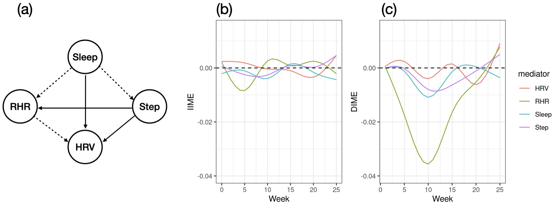
Figure 3: Analysis of IHS mobile health data: (a) the estimated DAG among the four mediators, dashed/solid arrows represent negative/positive effects; (b) the estimated intermediate individual mediation effects over time; (c) the estimated delayed individual mediation effects over time.

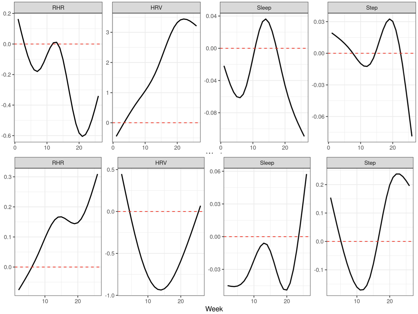
Figure 4: Analysis of IHS mobile health data: the estimated effects from the treatment to the four individual mediators, decomposed as the immediate (first row) and delayed (second row) effects, respectively.

We apply our method to this data. Figure 3(a) shows the estimated DAG structure among the four mediators, while Figures 3(b) and (c) show the estimated individual mediation effects over time that are smoothed with a natural cubic spline and further decomposed as the immediate and delayed effects. We make a number of observations. First of all, we see from Figure 3(a) that, the four mediators have complex relationships between each other, indicating the importance of accounting for the dependence structure among the mediators. Second, we see from Figures 3(b) and (c) that, the magnitude of the delayed effects is generally greater than that of the immediate effects, indicating the importance of accounting for the carryover effects in our understanding of the effects of push notification to intern’s mood. Finally, among all trajectories, we see that there is a strong carryover effect from push notification to mood score mediated by RHR. Figure 4 further plots the (smoothed) estimated effects from the treatment to the four individual mediators, decomposed as the immediate and delayed effects, respectively. We see that the push notification leads to an increased RHR after week five, suggesting that push notification can lead to a lower mood score by increasing the RHR. This agrees with our prior knowledge that an increased RHR usually indicates a more tired and stressful state, thus a worse mood.

In this supplement, we provide the proofs of the main theorems in the paper.

.1 Proof of Theorem 1

By Definition 1, the individual mediation effect of the $j$th mediator, $j=1,\ldots,d$, is of the form,

$$\eta_{j}^{(t)} = \frac{1}{t}\sum_{s=1}^{t}\frac{\partial}{\partial a}\mathbb{E}[R_{s}\mid do(A_{i}=a,\forall i\leq s)]-\frac{1}{t}\sum_{s=1}^{t}\frac{\partial}{\partial a}\mathbb{E}[R_{s}\mid do(A_{i}=a,M_{ij}=m,\forall i\leq s)]$$ (22)

$$= \frac{t-1}{t}\eta_{j}^{(t-1)}+\frac{1}{t}\left\{\frac{\partial}{\partial a}\mathbb{E}[R_{t}\mid do(A_{i}=a,\forall i\leq t)]-\frac{\partial}{\partial a}\mathbb{E}[R_{t}\mid do(A_{i}=a,M_{ij}=m,\forall i\leq t)]\right\}$$

$$= \frac{t-1}{t}\eta_{j}^{(t-1)}+\frac{1}{t}\left(\theta_{A_{1},\ldots,A_{t}\to R_{t}}-\theta_{A_{1},\ldots,A_{t}\to R_{t}}^{M_{1j},\ldots,M_{tj}}\right).$$

The key is to express (22) as a function of the intermediate quantities in Section 3.2 of the paper.

First, because all the treatments $(A_{1},\ldots,A_{t})$ are randomly assigned, and thus are independent of each other and all other covariates, we have

$$\theta_{A_{1},\ldots,A_{t}\to R_{t}} = \theta_{A_{1}\to R_{t}}+\theta_{A_{2}\to R_{t}}+\ldots+\theta_{A_{t}\to R_{t}},$$

$$\theta_{A_{1},\ldots,A_{t}\to R_{t}}^{M_{1j},\ldots,M_{tj}} = \theta_{A_{1}\to R_{t}}^{M_{1j},\ldots,M_{tj}}+\theta_{A_{2}\to R_{t}}^{M_{2j},\ldots,M_{tj}}+\ldots+\theta_{A_{t}\to R_{t}}^{M_{tj}}.$$

Next, we expand the terms in the summation of the second equation. Note that, when $s=t$, $\theta_{A_{t}\to R_{t}}^{M_{tj}}=\theta_{A_{t}\to R_{t}}-\theta_{A_{t}\to M_{tj}}\theta_{M_{tj}\to R_{t}}$. For any $s=1,\ldots,t-1$, the effect of $A_{s}$ to $R_{t}$ in a joint intervention on $(M_{sj},M_{(s+1)j}\ldots,M_{tj})$ is

$$\begin{split}\theta_{A_{s}\to R_{t}}^{M_{sj},\ldots,M_{tj}}&=\theta_{A_{s}\to R_{t}}^{M_{(s+1)j},\ldots,M_{tj}}-\theta_{A_{s}\to M_{sj}}\theta_{M_{sj}\to R_{t}}^{M_{(s+1)j},\ldots,M_{tj}}\\ &=\theta_{A_{s}\to R_{t}}^{M_{(s+2)j},\ldots,M_{tj}}-\theta_{A_{s}\to M_{(s+1)j}}\theta_{M_{(s+1)j}\to R_{t}}^{M_{(s+1)j},\ldots,M_{tj}}-\theta_{A_{s}\to M_{sj}}\theta_{M_{sj}\to R_{t}}^{M_{sj},\ldots,M_{tj}}\\ &=\ldots\\ &=\theta_{A_{s}\to R_{t}}-\sum_{i=s}^{t}\theta_{A_{s}\to M_{ij}}\theta_{M_{ij}\to R_{t}}^{M_{ij},\ldots,M_{tj}}.\end{split}$$ (23)

Next, we derive the recursive formula for computing $\theta_{M_{sj}\to R_{t}}^{M_{sj},\ldots,M_{tj}}$, with $s=1,\ldots,t-1$. The idea is similar to (23), i.e.,

$$\begin{split}\theta_{M_{sj}\to R_{t}}^{M_{sj},\ldots,M_{tj}}&=\theta_{M_{sj}\to R_{t}}^{M_{(s+2)j},\ldots,M_{tj}}-\theta_{M_{sj}\to M_{(s+1)j}}\theta_{M_{(s+1)j}\to R_{t}}^{M_{(s+1)j},\ldots,M_{tj}}\\ &=\theta_{M_{sj}\to R_{t}}^{M_{(s+3)j},\ldots,M_{tj}}-\theta_{M_{sj}\to M_{(s+2)j}}\theta_{M_{(s+2)j}\to R_{t}}^{M_{(s+2)j},\ldots,M_{tj}}-\theta_{M_{sj}\to M_{(s+1)j}}\theta_{M_{(s+1)j}\to R_{t}}^{M_{(s+1)j},\ldots,M_{tj}}\\ &=\ldots\\ &=\theta_{M_{sj}\to R_{t}}-\sum_{i=s+1}^{t}\theta_{M_{sj}\to M_{ij}}\theta_{M_{ij}\to R_{t}}^{M_{ij},\ldots,M_{tj}}.\end{split}$$ (24)

Given $\theta_{M_{ij}\to R_{t}}^{M_{ij},\ldots,M_{tj}}$ for $i=s+1,\ldots,t$, the above recursion allows us to evaluate $\theta_{M_{sj}\to R_{t}}^{M_{sj},\ldots,M_{tj}}$.

Given the expanded forms in (23) and (24), we compute the total effects from $(A_{1},\ldots,A_{t})$ on $R_{t}$ in a joint intervention on $(M_{1j},\ldots,M_{tj})$ as,

$$\theta_{A_{1},\ldots,A_{t}\to R_{t}}^{M_{1j},\ldots,M_{tj}} = \theta_{A_{1}\to R_{t}}^{M_{1j},\ldots,M_{tj}}+\theta_{A_{2}\to R_{t}}^{M_{2j},\ldots,M_{tj}}+\ldots+\theta_{A_{t}\to R_{t}}^{M_{tj}}$$

$$= \left(\theta_{A_{1}\to R_{t}}-\sum_{i=1}^{t}\theta_{A_{1}\to M_{ij}}\theta_{M_{ij}\to R_{t}}^{M_{ij},\ldots,M_{tj}}\right)+\left(\theta_{A_{2}\to R_{t}}-\sum_{i=2}^{t}\theta_{A_{2}\to M_{ij}}\theta_{M_{ij}\to R_{t}}^{M_{ij},\ldots,M_{tj}}\right)$$

$$\hskip 20.00003pt+\ldots+\left(\theta_{A_{t}\to R_{t}}-\theta_{A_{t}\to M_{tj}}\theta_{M_{ij}\to R_{t}}^{M_{ij},\ldots,M_{tj}}\right)$$

$$= \sum_{s=1}^{t}\theta_{A_{s}\to R_{t}}-\sum_{s=1}^{t}\sum_{i=s}^{t}\theta_{A_{s}\to M_{ij}}\theta_{M_{ij}\to R_{t}}^{M_{ij},\ldots,M_{tj}},$$

where $\theta_{M_{ij}\to R_{t}}^{M_{ij},\ldots,M_{tj}}$ can be calculated via (24).

Finally, we plug in the above expansion to (22), and obtain that,

$$\eta_{j}^{(t)}=\frac{1}{t}\left(\eta_{j}^{(t-1)}+\sum_{s=1}^{t}\sum_{i=s}^{t}\theta_{A_{s}\to M_{ij}}\theta_{M_{ij}\to R_{t}}^{M_{ij},\ldots,M_{tj}}\right),\ t=1,\ldots,T.$$

This completes the proof of Theorem 1. $\Box$

.2 Proof of Theorem 2

First, by the method of induction, we have,

$$\eta_{j}^{(1)} = \theta_{M_{1j}\to R_{1}}\theta_{A_{1}\to M_{1j}},$$

$$\eta_{j}^{(2)} = \frac{1}{2}\left\{\theta_{M_{1j}\to R_{1}}(2\theta_{A_{1}\to M_{1j}}+\theta_{A_{1}\to M_{2j}})+\theta_{M_{1j}\to R_{2}}^{M_{1j},M_{2j}}\theta_{A_{1}\to M_{1j}}\right\},$$

$$\eta_{j}^{(3)} = \frac{1}{3}\left\{\theta_{M_{1j}\to R_{1}}(3\theta_{A_{1}\to M_{1j}}+2\theta_{A_{1}\to M_{2j}}+\theta_{A_{1}\to M_{1j}})+\theta_{M_{1j}\to R_{3}}^{M_{1j},M_{2j},M_{3j}}\theta_{A_{1}\to M_{1j}}\right.$$

$$\quad\quad\quad\left.+\;\theta_{M_{1j}\to R_{2}}^{M_{1j},M_{2j}}(2\theta_{A_{1}\to M_{1j}}+\theta_{A_{1}\to M_{2j}})\right\},$$

$$\ldots$$

$$\eta_{j}^{(T)} = \frac{1}{T}\left[\theta_{M_{1j}\to R_{1}}\sum_{t=1}^{T}(T-t+1)\theta_{A_{1}\to M_{tj}}+\sum_{t=1}^{T-1}\theta_{M_{1j}\to R_{t+1}}^{M_{1j},\ldots,M_{(t+1)j}}\left\{\sum_{s=1}^{T-t}(T-t-s+1)\theta_{A_{1}\to M_{sj}}\right\}\right].$$

Taking $T\to\infty$ in the above formula of $\eta_{j}^{(T)}$, we have

$$\begin{split}\eta_{j}^{(\infty)}&=\theta_{M_{1j}\to R_{1}}\underset{T\to\infty}{\lim}\frac{1}{T}\sum_{t=1}^{T}(T-t+1)\theta_{A_{1}\to M_{tj}}+\underset{T\to\infty}{\lim}\frac{1}{T}\sum_{t=1}^{T-1}\theta_{M_{1j}\to R_{t+1}}^{M_{1j},\ldots,M_{(t+1)j}}\left\{\sum_{s=1}^{T-t}(T-t-s+1)\theta_{A_{1}\to M_{sj}}\right\}\\ &\equiv\theta_{M_{1j}\to R_{1}}I_{1j}+I_{2j}.\end{split}$$

We next derive the two terms $I_{1j}$ and $I_{2j}$, respectively,

For $I_{1j}$, we have

$$\begin{split}I_{1j}&=\lim_{T\to\infty}\frac{1}{T}\sum_{t=1}^{T}(T-t+1)\theta_{A_{1}\to M_{tj}}\\ &=\lim_{T\to\infty}\frac{1}{T}\left\{T\theta_{A_{1}\to M_{1j}}+(T-1)\theta_{A_{1}\to M_{2j}}+\ldots+\theta_{A_{1}\to M_{Tj}}\right\}\\ &=\lim_{T\to\infty}\frac{1}{T}\sum_{t=1}^{T}\sum_{s=1}^{t}\theta_{A_{1}\to M_{sj}}.\end{split}$$

Following the recursive relation in (14) of the paper, we first obtain the following equations with the time-invariant model parameters,

$$\begin{split}\bm{\theta}_{A_{1}\to\bm{M}_{1}}&=\bm{\delta}_{1},\\ \bm{\theta}_{A_{1}\to\bm{M}_{2}}&=\bm{\Gamma}_{1}\bm{\theta}_{A_{1}\to\bm{M}_{1}}+\bm{\zeta}_{1}\theta_{A_{1}\to R_{1}},\\ &\ldots\\ \bm{\theta}_{A_{1}\to\bm{M}_{t}}&=\bm{\Gamma}_{1}\bm{\theta}_{A_{1}\to\bm{M}_{t-1}}+\bm{\zeta}_{1}\theta_{A_{1}\to R_{t-1}}.\end{split}$$

Taking summation over the above equations leads to

$$\sum_{s=1}^{t}\bm{\theta}_{A_{1}\to\bm{M}_{s}}=\bm{\delta}_{1}+\bm{\Gamma}_{1}\sum_{s=1}^{t-1}\bm{\theta}_{A_{1}\to\bm{M}_{s}}+\bm{\zeta}_{1}\sum_{s=1}^{t-1}\theta_{A_{1}\to R_{s}}.$$

Taking another summation of the above equations leads to

$$\frac{1}{T}\sum_{t=2}^{T}\sum_{s=1}^{t}\bm{\theta}_{A_{1}\to\bm{M}_{s}}=\frac{T-1}{T}\bm{\delta}_{1}+\bm{\Gamma}_{1}\frac{1}{T}\sum_{t=1}^{T-1}\sum_{s=1}^{t}\bm{\theta}_{A_{1}\to\bm{M}_{s}}+\bm{\zeta}_{1}\frac{1}{T}\sum_{t=1}^{T-1}\sum_{s=1}^{t}\theta_{A_{1}\to R_{s}}.$$ (25)

Similarly, to evaluate $\sum_{s=1}^{t}\theta_{A_{1}\to R_{s}}$, we first obtain the recursion relations,

$$\begin{split}\theta_{A_{1}\to R_{1}}&=\delta_{2}+\bm{\kappa}^{\mbox{\tiny{\sf T}}}\bm{\theta}_{A_{1}\to\bm{M}_{1}},\\ \theta_{A_{1}\to R_{2}}&=\zeta_{2}\theta_{A_{1}\to R_{1}}+\bm{\kappa}^{\mbox{\tiny{\sf T}}}\bm{\theta}_{A_{1}\to\bm{M}_{2}}+\bm{\gamma}_{2}^{\mbox{\tiny{\sf T}}}\bm{\theta}_{A_{1}\to\bm{M}_{1}},\\ &\ldots\\ \theta_{A_{1}\to R_{t}}&=\zeta_{2}\theta_{A_{1}\to R_{t-1}}+\bm{\kappa}^{\mbox{\tiny{\sf T}}}\bm{\theta}_{A_{1}\to\bm{M}_{t}}+\bm{\gamma}_{2}^{\mbox{\tiny{\sf T}}}\bm{\theta}_{A_{1}\to\bm{M}_{t-1}}.\end{split}$$

Taking double summation over the above equations leads to

$$\frac{1}{T}\sum_{t=2}^{T}\sum_{s=1}^{t}\theta_{A_{1}\to R_{s}}=\frac{T-1}{T}\delta_{2}+\zeta_{2}\frac{1}{T}\sum_{t=1}^{T-1}\sum_{s=1}^{t}\theta_{A_{1}\to R_{s}}+\bm{\kappa}^{\mbox{\tiny{\sf T}}}\frac{1}{T}\sum_{t=1}^{T-1}\sum_{s=1}^{t}\bm{\theta}_{A_{1}\to\bm{M}_{s}}+\bm{\gamma}_{2}^{\mbox{\tiny{\sf T}}}\frac{1}{T}\sum_{t=1}^{T-1}\sum_{s=1}^{t}\bm{\theta}_{A_{1}\to\bm{M}_{s}}$$ (26)

Denote ${\bm{B}}_{1}\equiv\lim_{T\to\infty}T^{-1}\sum_{t=2}^{T}\sum_{s=1}^{t}\bm{\theta}_{A_{1}\to\bm{M}_{s}}\in\mathbb{R}^{d}$, and $\widetilde{R}\equiv\lim_{T\to\infty}T^{-1}\sum_{t=2}^{T}\sum_{s=1}^{t}\theta_{A_{1}\to R_{s}}$. Combining (25) and (26), we obtain that

$$\begin{split}\bm{B}_{1}&=\bm{\delta}_{1}+\bm{\Gamma}_{1}\bm{B}_{1}+\bm{\zeta}_{1}\widetilde{R},\\ \widetilde{R}&=\delta_{2}+\zeta_{2}\widetilde{R}+\bm{\kappa}^{\mbox{\tiny{\sf T}}}\bm{B}_{1}+\bm{\gamma}_{2}^{\mbox{\tiny{\sf T}}}\bm{B}_{1}.\end{split}$$

Solving the above equations leads to

$$\bm{B}_{1}=\left\{(1-\zeta_{2})(\bm{\mathrm{I}}-\bm{\Gamma}_{1})-\bm{\zeta}_{1}(\bm{\kappa}+\bm{\gamma}_{2})^{\mbox{\tiny{\sf T}}}\right\}^{-1}\left\{(1-\zeta_{2})\bm{\delta}_{1}+\delta_{2}\bm{\zeta}_{1}\right\}.$$

Then $I_{1j}$ is the $j$th element in the vector ${\bm{B}}_{1}$.

For $I_{2j}$, we have

$$\begin{split}I_{2j}&=\underset{T\to\infty}{\lim}\frac{1}{T}\sum_{t=1}^{T-1}\theta_{M_{1j}\to R_{t+1}}^{M_{1j},\ldots,M_{(t+1)j}}\left\{\sum_{s=1}^{T-t}(T-t-s+1)\theta_{A_{1}\to M_{sj}}\right\}\\ &=\underset{T\to\infty}{\lim}\frac{1}{T}\sum_{t=1}^{T-1}\theta_{M_{1j}\to R_{t+1}}^{M_{1j},\ldots,M_{(t+1)j}}\left(\sum_{s=1}^{T-t}\sum_{i=1}^{s}\theta_{A_{1}\to M_{ij}}\right).\end{split}$$

For notational simplicity, let $L_{tj}\equiv\sum_{s=1}^{t}\sum_{i=1}^{s}\theta_{A_{1}\to M_{ij}}$. Next, we derive the recursive relationship for the summation $T^{-1}\sum_{t=1}^{T-1}\theta_{M_{1j}\to R_{t+1}}^{M_{1j},\ldots,M_{(t+1)j}}L_{(T-t)j}$.

Following the recursion for $\theta_{M_{sj}\to R_{t}}^{M_{sj},\ldots,M_{tj}}$ in (24), and multiplying both sides by $L_{tj}$, we obtain that

$$\begin{split}\theta_{M_{1j}\to R_{2}}^{M_{1j},M_{2j}}L_{(T-1)j}&=L_{(T-1)j}\theta_{M_{1j}\to R_{2}}-\theta_{M_{1j}\to M_{2j}}\theta_{M_{1j}\to R_{1}}L_{(T-1)j},\\ \theta_{M_{1j}\to R_{3}}^{M_{1j},\ldots,M_{3j}}L_{(T-2)j}&=L_{(T-2)j}\theta_{M_{1j}\to R_{3}}-\theta_{M_{1j}\to M_{3j}}\theta_{M_{1j}\to R_{1}}L_{(T-2)j}-\theta_{M_{1j}\to M_{2j}}\theta_{M_{1j}\to R_{2}}^{M_{1j},M_{2j}}L_{(T-2)j},\\ \theta_{M_{1j}\to R_{4}}^{M_{1j},\ldots,M_{4j}}L_{(T-3)j}&=L_{(T-3)j}\theta_{M_{1j}\to R_{4}}-\theta_{M_{1j}\to M_{4j}}\theta_{M_{1j}\to R_{1}}L_{(T-3)}-\sum_{i=2}^{3}\theta_{M_{1j}\to M_{ij}}\theta_{M_{1j}\to R_{4-i+1}}^{M_{1j},\ldots,M_{(4-i+1)j}}L_{(T-3)j},\\ &\ldots\\ \theta_{M_{1j}\to R_{T}}^{M_{1j},\ldots,M_{Tj}}L_{1j}&=L_{1j}\theta_{M_{1j}\to R_{T}}-\theta_{M_{1j}\to M_{Tj}}\theta_{M_{1j}\to R_{1}}L_{1j}-\sum_{i=2}^{T-1}\theta_{M_{1j}\to M_{ij}}\theta_{M_{1j}\to R_{T-i+1}}^{M_{1j},\ldots,M_{(T-i+1)j}}L_{1j}.\end{split}$$

Taking summation over the above equations leads to

$$\begin{split}\frac{1}{T}\sum_{t=1}^{T-1}\theta_{M_{1j}\to R_{t+1}}^{M_{1j},\ldots,M_{(t+1)j}}L_{(T-t)j}&=\frac{1}{T}\sum_{t=1}^{T-1}\theta_{M_{1j}\to R_{t}}L_{(T-t)j}-\theta_{M_{1j}\to R_{1}}\frac{1}{T}\sum_{t=1}^{T-1}\theta_{M_{1j}\to M_{tj}}L_{(T-t)j}\\ &-\sum_{i=2}^{T-1}\theta_{M_{1j}\to M_{ij}}\frac{1}{T}\sum_{t=1}^{T-i}\theta_{M_{1j}\to R_{t+1}}^{M_{1j},\ldots,M_{(t+1)j}}L_{(T-i-t+1)j}.\end{split}$$

Define ${\bm{B}}_{2}\equiv\lim_{T\to\infty}\sum_{t=2}^{T}\bm{\theta}_{M_{1j}\to\bm{M}_{t}}\in\mathbb{R}^{d}$, $B_{3j}\equiv\lim_{T\to\infty}\sum_{t=2}^{T}\theta_{M_{1j}\to R_{t}}$, ${\bm{B}}_{4}\equiv\lim_{T\to\infty}T^{-1}\sum_{t=2}^{T}$ $\bm{\theta}_{M_{1j}\to\bm{M}_{t}}L_{(T-t+1)j}$, and $B_{5j}\equiv\lim_{T\to\infty}T^{-1}\sum_{t=2}^{T}\theta_{M_{1j}\to R_{t}}L_{(T-t+1)j}$. Taking the limit with $T\to\infty$ on both sides of the above equation leads to

$$I_{2j}=(1+B_{2j})^{-1}(B_{5j}-\theta_{M_{1j}\to R_{1}}B_{4j}).$$ (27)

Next, we obtain the recursive relationship for $\sum_{t=2}^{T}\bm{\theta}_{M_{1j}\to\bm{M}_{t}}$, $\sum_{t=2}^{T}\bm{\theta}_{M_{1j}\to\bm{M}_{t}}L_{(T-t+1)j}$, and $\sum_{t=2}^{T}\theta_{M_{1j}\to R_{t}}L_{(T-t+1)j}$. Let $\bm{B}_{6}\equiv\begin{pmatrix}\bm{0}_{d\times d}&\bm{0}_{d}\\ \bm{\kappa}^{\mbox{\tiny{\sf T}}}&0\end{pmatrix}$ and $\bm{B}_{7}\equiv\begin{pmatrix}\bm{\Gamma}_{1}&\bm{\zeta}_{1}\\ \bm{\gamma}_{2}^{\mbox{\tiny{\sf T}}}&\zeta_{2}\end{pmatrix}$. The recursion between $(\bm{\theta}_{M_{1j}\to\bm{M}_{t}},\theta_{M_{1j}\to R_{t}})$ and $(\bm{\theta}_{M_{1j}\to\bm{M}_{t-1}},\theta_{M_{1j}\to R_{t-1}})$ takes the following form:

$$\begin{bmatrix}\bm{\theta}_{M_{1j}\to\bm{M}_{t}}\\ \theta_{M_{1j}\to R_{t}}\end{bmatrix}=\begin{pmatrix}\bm{0}_{d\times d}&\bm{0}_{d}\\ \bm{\kappa}^{\mbox{\tiny{\sf T}}}&0\end{pmatrix}\begin{bmatrix}\bm{\theta}_{M_{1j}\to\bm{M}_{t}}\\ \theta_{M_{1j}\to R_{t}}\end{bmatrix}+\begin{pmatrix}\bm{\Gamma}_{1}&\bm{\zeta}_{1}\\ \bm{\gamma}_{2}^{\mbox{\tiny{\sf T}}}&\zeta_{2}\end{pmatrix}\begin{bmatrix}\bm{\theta}_{M_{1j}\to\bm{M}_{t-1}}\\ \theta_{M_{1j}\to R_{t-1}}\end{bmatrix}$$ (28)

Taking summation from $t=2$ to $T$ of the above equation leads to

$$\sum_{t=2}^{T}(\bm{\mathrm{I}}-\bm{B}_{6})\begin{bmatrix}\bm{\theta}_{M_{1j}\to\bm{M}_{t}}\\ \theta_{M_{1j}\to R_{t}}\end{bmatrix}=\sum_{t=2}^{T}\bm{B}_{7}\begin{bmatrix}\bm{\theta}_{M_{1j}\to\bm{M}_{t-1}}\\ \theta_{M_{1j}\to R_{t-1}}\end{bmatrix}$$

$$(\bm{\mathrm{I}}-\bm{B}_{6})\sum_{t=2}^{T}\begin{bmatrix}\bm{\theta}_{M_{1j}\to\bm{M}_{t}}\\ \theta_{M_{1j}\to R_{t}}\end{bmatrix}=\bm{B}_{7}\sum_{t=2}^{T-1}\begin{bmatrix}\bm{\theta}_{M_{1j}\to\bm{M}_{t}}\\ \theta_{M_{1j}\to R_{t}}\end{bmatrix}+\bm{B}_{7}\begin{bmatrix}\bm{\theta}_{M_{1j}\to\bm{M}_{1}}\\ \theta_{M_{1j}\to R_{1}}\end{bmatrix}$$

Taking the limit with $T\to\infty$ on both sides leads to

$$\begin{bmatrix}\bm{B}_{2}\\ B_{3j}\end{bmatrix}=(\bm{\mathrm{I}}-\bm{B}_{6}-\bm{B}_{7})^{-1}\bm{B}_{7}\begin{bmatrix}\bm{\theta}_{M_{1j}\to\bm{M}_{1}}\\ \theta_{M_{1j}\to R_{1}}\end{bmatrix}.$$ (29)

Multiply both sides of the recursion in (28) by $L_{(T-t+1)j}$ leads to

$$\begin{bmatrix}\bm{\theta}_{M_{1j}\to\bm{M}_{t}}L_{(T-t+1)j}\\ \theta_{M_{1j}\to R_{t}}L_{(T-t+1)j}\end{bmatrix} =\bm{B}_{6}\begin{bmatrix}\bm{\theta}_{M_{1j}\to\bm{M}_{t}}L_{(T-t+1)j}\\ \theta_{M_{1j}\to R_{t}}L_{(T-t+1)j}\end{bmatrix}+\bm{B}_{7}\begin{bmatrix}\bm{\theta}_{M_{1j}\to\bm{M}_{t-1}}L_{(T-t+1)j}\\ \theta_{M_{1j}\to R_{t-1}}L_{(T-t+1)j}\end{bmatrix},$$

$$\frac{1}{T}\sum_{t=2}^{T}(\bm{\mathrm{I}}-\bm{B}_{6})\begin{bmatrix}\bm{\theta}_{M_{1j}\to\bm{M}_{t}}L_{(T-t+1)j}\\ \theta_{M_{1j}\to R_{t}}L_{(T-t+1)j}\end{bmatrix} =\frac{1}{T}\sum_{t=2}^{T}\bm{B}_{7}\begin{bmatrix}\bm{\theta}_{M_{1j}\to\bm{M}_{t-1}}L_{(T-t+1)j}\\ \theta_{M_{1j}\to R_{t-1}}L_{(T-t+1)j}\end{bmatrix}$$

$$(\bm{\mathrm{I}}-\bm{B}_{6}-\bm{B}_{7})\frac{1}{T}\sum_{t=2}^{T}\begin{bmatrix}\bm{\theta}_{M_{1j}\to\bm{M}_{t}}L_{(T-t+1)j}\\ \theta_{M_{1j}\to R_{t}}L_{(T-t+1)j}\end{bmatrix} =\frac{1}{T}\bm{B}_{7}\begin{bmatrix}\bm{\theta}_{M_{1j}\to\bm{M}_{1}}L_{(T-1)j}\\ \theta_{M_{1j}\to R_{1}}L_{(T-1)j}\end{bmatrix}$$

Furthermore, we have $\lim_{T\to\infty}\frac{1}{T}L_{(T-1)j}=\lim_{T\to\infty}\frac{1}{T}\sum_{t=1}^{T-1}\sum_{i=1}^{t}\theta_{A_{1}\to M_{ij}}=B_{1j}$. We now take the limit with $T\to\infty$ on both sides of the summations, we have

$$\begin{bmatrix}\bm{B}_{4}\\ B_{5j}\end{bmatrix}=(\bm{\mathrm{I}}-\bm{B}_{6}-\bm{B}_{7})^{-1}\bm{B}_{7}\begin{bmatrix}\bm{\theta}_{M_{1j}\to\bm{M}_{1}}\\ \theta_{M_{1j}\to R_{1}}\end{bmatrix}B_{1j}.$$ (30)

We then combine (27), (29) and (30) and solve for $I_{2j}$.

This completes the proof of Theorem 2. $\Box$

.3 Proof of Theorem 3

We begin with some notations. Let $\text{vech}(\bm{B})\in\mathbb{R}^{q(q+1)/2}$ denote the half-vectorization of a symmetric $q\times q$ matrix $\bm{B}$ that vectorizes the lower triangular part of $\bm{B}$. Let $\bm{e}_{r}$ denote the $r$th column of an identity matrix, and $\text{diag}(\bm{B})$ the diagonal matrix whose diagonal is the same as the diagonal of the matrix $\bm{B}$. Let ${\partial\bm{y}}/{\partial\bm{x}}$ denote the $r\times s$ matrix of the derivative of $\bm{y}(\bm{x})=\left(y_{1}(\bm{x}),\ldots,y_{r}(\bm{x})\right)^{\mbox{\tiny{\sf T}}}\in\mathbb{R}^{r}$ with respect to $\bm{x}=(x_{1},\ldots,x_{s})^{\mbox{\tiny{\sf T}}}\in\mathbb{R}^{s}$ whose $(i,j)$th entry is ${\partial y_{i}}/{\partial x_{j}},i=1,\ldots,r,j=1,\ldots,s$.

We first prove the case of $T=1$, then the case of $T=2$. The case for any finite $T>2$ can be proved in a similar fashion.

For $T=1$, recall $\eta_{j}^{(1)}=\theta_{A_{1}\to M_{1j}}\theta_{M_{1j}\to R_{1}}=\beta_{1j}\beta_{M_{1j},R_{1}\mid\mathrm{Pa}_{j}\cup A_{1}}$, and $\widehat{\eta}_{j}^{(1)}=\widehat{\theta}_{A_{1}\to M_{1j}}\widehat{\theta}_{M_{1j}\to R_{1}}=\widehat{\beta}_{1j}\widehat{\beta}_{M_{1j},R_{1}\mid\mathrm{Pa}_{j}\cup A_{1}}$ as $n\to\infty$. To establish the asymptotic distribution of $\widehat{\eta}_{j}^{(1)}$, the main idea is to first show the asymptotic distribution of $(\widehat{\theta}_{A_{1}\to M_{1j}},\widehat{\theta}_{M_{1j}\to R_{1}})^{\mbox{\tiny{\sf T}}}$, then apply the delta method.

Let $\bm{U}_{1}\equiv(U_{11},\ldots,U_{1q_{1}})^{\mbox{\tiny{\sf T}}}=(A_{1},\mathrm{Pa}_{1j}^{\mbox{\tiny{\sf T}}},M_{1j},R_{1})^{\mbox{\tiny{\sf T}}}\in\mathbb{R}^{q_{1}}$. Let $\bm{\Sigma}_{1}=\text{cov}(\bm{U}_{1})\in\mathbb{R}^{q_{1}\times q_{1}}$, and let $\widehat{\bm{\Sigma}}_{1}$ denote the corresponding sample covariance matrix. Since all fourth moments of the variables in $\bm{U}_{1}$ are finite, the central limit theorem implies that

$$\sqrt{n}\left\{\text{vech}(\widehat{\bm{\Sigma}}_{1})-\text{vech}(\bm{\Sigma}_{1})\right\}\overset{d}{\to}\mathcal{N}(\bm{0},\bm{V}_{1}),$$ (31)

where $\bm{V}_{1}=\text{cov}\left(\text{vech}(\bm{U}_{1}\bm{U}_{1}^{\mbox{\tiny{\sf T}}})\right)$.

Let $\bm{\theta}_{1}\equiv(\theta_{A_{1}\to M_{1j}},\theta_{M_{1j}\to R_{1}})^{\mbox{\tiny{\sf T}}}=(\beta_{1j},\beta_{M_{1j},R_{1}\mid\mathrm{Pa}_{1j}\cup A_{1}})^{\mbox{\tiny{\sf T}}}$, and $\widehat{\bm{\theta}}_{1}\equiv(\widehat{\theta}_{A_{1}\to M_{1j}},\widehat{\theta}_{M_{1j}\to R_{1}})^{\mbox{\tiny{\sf T}}}=(\widehat{\beta}_{1j},\widehat{\beta}_{M_{1j},R_{1}\mid\mathrm{Pa}_{1j}\cup A_{1}})^{\mbox{\tiny{\sf T}}}$. There exists a differentiable function $h_{11}:\mathbb{R}^{q_{1}(q_{1}+1)/2}\to\mathbb{R}^{2}$, such that $h_{11}(\text{vech}(\bm{\Sigma}_{1}))=\bm{\theta}_{1}$, and $h_{11}(\text{vech}(\widehat{\bm{\Sigma}}_{1}))=\widehat{\bm{\theta}}_{1}$. Therefore, by (31) and the multivariate delta method, we have

$$\sqrt{n}(\widehat{\bm{\theta}}_{1}-\bm{\theta}_{1})\overset{d}{\to}\mathcal{N}(\bm{0},\bm{\Lambda}_{1}\bm{V}_{1}\bm{\Lambda}_{1}^{\mbox{\tiny{\sf T}}}),$$

where $\bm{\Lambda}_{1}=\partial\bm{\theta}_{1}/\partial\text{vech}(\bm{\Sigma}_{1})$.

Consider another differentiable function $h_{12}(x_{1},x_{2})=x_{1}x_{2}$, and apply the multivariate delta method again, we have

$$\sqrt{n}(\widehat{\eta}_{j}^{(1)}-\eta_{j}^{(1)})\overset{d}{\to}\mathcal{N}(0,\bm{S}_{1}\bm{\Lambda}_{1}\bm{V}_{1}\bm{\Lambda}_{1}^{\mbox{\tiny{\sf T}}}\bm{S}_{1}^{\mbox{\tiny{\sf T}}}),$$

where $\bm{V}_{1}=\text{cov}\left(\text{vech}(\bm{U}_{1}\bm{U}_{1}^{\mbox{\tiny{\sf T}}})\right)$, $\bm{\Lambda}_{1}=\partial\bm{\theta}_{1}/\partial\left(\text{vech}(\bm{\Sigma}_{1})\right)$, $\bm{\theta}_{1}=(\theta_{A_{1}\to M_{1j}},\theta_{M_{1j}\to R_{1}})^{\mbox{\tiny{\sf T}}}$, and $\bm{S}_{1}={\partial\eta_{j}^{(1)}}/{\partial\bm{\theta}_{1}}$.

For $T=2$, let $\bm{U}_{2}\equiv(U_{21},\ldots,U_{2q_{2}})^{\mbox{\tiny{\sf T}}}=(A_{1},\bm{M}_{1}^{\mbox{\tiny{\sf T}}},R_{1},A_{2},\mathrm{Pa}_{2j}^{\mbox{\tiny{\sf T}}},M_{2j},R_{2})^{\mbox{\tiny{\sf T}}}\in\mathbb{R}^{q_{2}}$, where $\mathrm{Pa}_{2j}=\{M_{2i}:(\bm{W}_{t})_{ij}\neq 0,i\in\{1,\ldots,d\}\setminus\{j\}\}$ is the parent set of $M_{2j}$ in $\mathcal{G}_{2}$. Let $\bm{\Sigma}_{2}=\text{cov}(\bm{U}_{2})\in\mathbb{R}^{q_{2}\times q_{2}}$ and let $\widehat{\bm{\Sigma}}_{2}$ denote the corresponding sample covariance matrix. Similar to (31), we have

$$\sqrt{n}\left\{\text{vech}(\widehat{\bm{\Sigma}}_{2})-\text{vech}(\bm{\Sigma}_{2})\right\}\overset{d}{\to}\mathcal{N}(\bm{0},\bm{V}_{2}),$$

where $\bm{V}_{2}=\text{cov}\left(\text{vech}(\bm{U}_{2}\bm{U}_{2}^{\mbox{\tiny{\sf T}}})\right)$.

Let $\bm{\theta}_{2}\equiv(\theta_{A_{1}\to M_{1j}},\theta_{M_{1j}\to R_{1}},\theta_{A_{1}\to M_{2j}},\theta_{M_{1j}\to{M_{2j}}},\theta_{M_{1j}\to R_{2}},\theta_{A_{2}\to M_{2j}},\theta_{M_{2j}\to R_{2}})^{\mbox{\tiny{\sf T}}}$, and $\widehat{\bm{\theta}}_{2}\equiv(\widehat{\theta}_{A_{1}\to M_{1j}},$ $\widehat{\theta}_{M_{1j}\to R_{1}},\widehat{\theta}_{A_{1}\to M_{2j}},\widehat{\theta}_{M_{1j}\to{M_{2j}}},\widehat{\theta}_{M_{1j}\to R_{2}},\widehat{\theta}_{A_{2}\to M_{2j}},\widehat{\theta}_{M_{2j}\to R_{2}})^{\mbox{\tiny{\sf T}}}$. Note that every element in $\bm{\theta}_{2}$ represents the total effect of one variable on another, where all variables in this expanded DAG up to the second stage are included in $\bm{U}_{2}$. For example, $\theta_{M_{1j}\to R_{2}}=\beta_{M_{1j},R_{2}\mid\mathrm{Pa}_{j}\cup A_{1}}$ where this regression coefficient depends only on the covariance matrix of $\bm{U}_{2}$, which is $\bm{\Sigma}_{2}$. Then there exists a differentiable function $h_{21}:\mathbb{R}^{q_{2}(q_{2}+1)/2}\to\mathbb{R}^{7}$, such that $h_{21}(\text{vech}(\bm{\Sigma}_{2}))=\bm{\theta}_{2}$ and $h_{21}(\text{vech}(\widehat{\bm{\Sigma}}_{2}))=\widehat{\bm{\theta}}_{2}$. By the multivariate delta method, we have

$$\sqrt{n}(\widehat{\bm{\theta}}_{2}-\bm{\theta}_{2})\overset{d}{\to}\mathcal{N}(\bm{0},\bm{\Lambda}_{2}\bm{V}_{2}\bm{\Lambda}_{2}^{\mbox{\tiny{\sf T}}}),$$

where $\bm{\Lambda}_{2}={\partial\bm{\theta}_{2}}/{\partial\left(\text{vech}(\bm{\Sigma}_{2})\right)}$.

Consider another differentiable function $h(x_{1},x_{2},\ldots,x_{7})=\{x_{1}x_{2}+(x_{3}+x_{6})\cdot x_{7}+x_{1}(x_{5}-x_{4}x_{7})\}/2$, and apply the multivariate delta method again, we have

$$\sqrt{n}(\widehat{\eta}_{j}^{(2)}-\eta_{j}^{(2)})\overset{d}{\to}\mathcal{N}(0,\bm{S}_{2}\bm{\Lambda}_{2}\bm{V}_{2}\bm{\Lambda}_{2}^{\mbox{\tiny{\sf T}}}\bm{S}_{2}^{\mbox{\tiny{\sf T}}}),$$

where $\bm{V}_{2}=\text{cov}\left(\text{vech}(\bm{U}_{2}\bm{U}_{2}^{\mbox{\tiny{\sf T}}})\right)$, $\bm{\Lambda}_{2}=\partial\bm{\theta}_{2}/\partial\left(\text{vech}(\bm{\Sigma}_{2})\right)$, and $\bm{S}_{2}={\partial\eta_{j}^{(2)}}/{\partial\bm{\theta}_{2}}$.

This completes the proof of Theorem 3. $\Box$

.4 Proof of Theorem 4

From the proof of Theorem 2, recall that $I_{1j}=B_{1j}$, and $I_{2j}=(1+{B}_{2j})^{-1}(B_{5j}-\theta_{M_{1j}\to R_{1}}B_{4j})$. Therefore, $I_{1j}$, $I_{2j}$ are continuous functions of the intermediate quantities $(\theta_{M_{1j}\to R_{1}},\bm{\theta}_{M_{1j}\to\bm{M}_{1}})$, and the model parameters $\bm{\Theta}_{1}=(\bm{\alpha}_{1},\bm{\beta}_{1},\bm{\Gamma}_{1},\bm{\zeta}_{1})^{\mbox{\tiny{\sf T}}}\in\mathbb{R}^{(d+3)\times d}$, $\bm{\Theta}_{2}=(\alpha_{2},\beta_{2},\zeta_{2},\bm{\gamma}_{2}^{\mbox{\tiny{\sf T}}},\bm{\kappa}^{\mbox{\tiny{\sf T}}})^{\mbox{\tiny{\sf T}}}\in\mathbb{R}^{(2d+3)\times 1}$. To establish the asymptotic distribution of $\widehat{\eta}_{j}^{(\infty)}=\widehat{\theta}_{M_{1j}\to R_{1}}\widehat{I}_{1j}+\widehat{I}_{2j}$, the main idea is to first show the asymptotic distribution of the estimators of the model parameters $(\bm{\Theta}_{1},\bm{\Theta}_{2})$ and those intermediate quantities $(\bm{B}_{1},\bm{B}_{2},B_{3j},\bm{B}_{4},B_{5j})$, then apply the delta method.

We first show the asymptotic normality of $\widehat{\bm{\Theta}}_{2}$. The asymptotic normality of $\widehat{\bm{\Theta}}_{1}$ can be shown similarly. Let $\bm{X}_{t}\equiv({1},A_{t},\bm{M}_{t-1}^{\mbox{\tiny{\sf T}}},R_{t-1},\bm{M}_{t}^{\mbox{\tiny{\sf T}}})^{\mbox{\tiny{\sf T}}}\in\mathbb{R}^{(2d+3)\times 1}$. Since

$$\sqrt{T}(\widehat{\bm{\Theta}}_{2}-\bm{\Theta}_{2})=\left(\frac{1}{T}\sum_{t=1}^{T}\bm{X}_{t}\bm{X}_{t}^{\mbox{\tiny{\sf T}}}\right)^{-1}\left(\frac{1}{\sqrt{T}}\sum_{t=1}^{T}\bm{X}_{t}\epsilon_{rt}\right),$$

and the stochastic process $\{(A_{t},\bm{M}_{t}^{\mbox{\tiny{\sf T}}},R_{t}):t\geq 1\}$ is $\beta$-mixing, by the weak law of large numbers of a weak mixing process, we have

$$\begin{split}&\frac{1}{T}\sum_{t=1}^{T}\bm{X}_{t}\bm{X}_{t}^{\mbox{\tiny{\sf T}}}\overset{p}{\to}\mathbb{E}[\bm{X}_{0}\bm{X}_{0}^{\mbox{\tiny{\sf T}}}],\ \text{where}\ \mathbb{E}[\bm{X}_{0}\bm{X}_{0}^{\mbox{\tiny{\sf T}}}]=\lim_{T\to\infty}\frac{1}{T}\sum_{t=1}^{T}\mathbb{E}[\bm{X}_{t}\bm{X}_{t}^{\mbox{\tiny{\sf T}}}],\\ &\frac{1}{T}\sum_{t=1}^{T}\bm{X}_{t}\epsilon_{rt}\overset{p}{\to}\bm{0},\text{because}\ \bm{X}_{t}\;\,\rule[0.0pt]{0.29999pt}{6.69998pt}\rule[-0.20004pt]{6.99997pt}{0.29999pt}\rule[0.0pt]{0.29999pt}{6.69998pt}\;\,\epsilon_{rt},\ \text{and}\ \mathbb{E}[\epsilon_{rt}]={0}.\end{split}$$

Next, we derive the asymptotic distribution of $\widetilde{\bm{U}}_{T}=\sum_{t=1}^{T}\bm{U}_{t}\equiv\sum_{t=1}^{T}\bm{X}_{t}\epsilon_{rt}\in\mathbb{R}^{(2d+3)\times 1}$. To apply the Cramér-Wold theorem, let $\bm{a}=(a_{1},\ldots,a_{2d+3})^{\mbox{\tiny{\sf T}}}\in\mathbb{R}^{2d+3}$ be a nonrandom and nonzero vector, and $\bm{U}_{t}=(U_{t1},\ldots,U_{t,2d+3})^{\mbox{\tiny{\sf T}}}$. Then we write

$$\bm{a}^{\mbox{\tiny{\sf T}}}\widetilde{\bm{U}}_{T}=\sum_{t=1}^{T}\sum_{p=1}^{2d+3}a_{p}U_{tp}=\sum_{t=1}^{T}U_{t}^{\prime}.$$

Since $\{\bm{U}_{t}\}_{t\geq 1}$ is a $\beta$-mixing process with mean zero, it follows that $\{U_{t}^{\prime}\}_{t\geq 1}$ is also a $\beta$-mixing centered process with the second moment given by

$$\sigma^{2}_{T}=\bm{a}^{\mbox{\tiny{\sf T}}}\text{var}(\widetilde{\bm{U}}_{T})\bm{a}=\text{var}\left(\sum_{t=1}^{T}U_{t}^{\prime}\right)\to\infty,\ T\to\infty.$$

For every $\epsilon>0$,

$$\begin{split}\sum_{t=1}^{T}\mathbb{E}\left[(U_{t}^{\prime})^{2}\mathbf{1}(|U_{t}^{\prime}|>\epsilon\sigma_{T})\right]&=\sum_{t=1}^{T}\mathbb{E}\left\{\left(\sum_{p=1}^{2d+3}a_{p}U_{tp}\right)^{2}\mathbf{1}\left(\sum_{p=1}^{2d+3}|a_{p}U_{tp}|>\epsilon\sigma_{T}\right)\right\}\\ &\leq\sum_{t=1}^{T}a_{p}^{2}\mathbb{E}\left\{U_{tp}^{2}\mathbf{1}\left(\sum_{p=1}^{2d+3}|U_{tp}|>\frac{\epsilon\sigma_{T}}{\max_{p}|a_{p}|}\right)\right\},\end{split}$$

where $\mathbf{1}(\cdot)$ is an indicator function. Since $\sigma_{T}\to\infty$, and $\max_{p}|a_{p}|<\infty$, we have

$$\mathbf{1}\left(\sum_{p=1}^{2d+3}|U_{tp}|>\frac{\epsilon\sigma_{T}}{\max_{p}|a_{p}|}\right)\overset{a.s.}{\to}0.$$

In addition, because $\mathbb{E}[U_{tp}^{2}]<\infty$, and $\mathbb{P}(U_{tp}=\infty)=0$, it follows that

$$\sum_{t=1}^{T}\mathbb{E}\left[(U_{t}^{\prime})^{2}\mathbf{1}(|U_{t}^{\prime}|>\epsilon\sigma_{T})\right]\to 0,\ T\to\infty.$$

By the central limit theorem for martingales, we have

$$\frac{\sum_{t=1}^{T}U_{t}^{\prime}}{\sigma_{T}}\overset{d}{\to}\mathcal{N}(0,1),\ \text{as}\ T\to\infty.$$

Applying the Cramér-Wold theorem, we have

$$\begin{split}\frac{1}{\sqrt{T}}\sum_{t=1}^{T}\bm{U}_{t}=\frac{1}{\sqrt{T}}\sum_{t=1}^{T}\bm{X}_{t}\epsilon_{rt}\overset{d}{\to}\mathcal{N}(\bm{0},\bm{V}_{r}),\end{split}$$

where $\bm{V}_{r}=\sigma_{r}^{2}\mathbb{E}(\bm{X}_{t}\bm{X}_{t}^{\mbox{\tiny{\sf T}}})\in\mathbb{R}^{(2d+3)\times(2d+3)}$. By Slutsky’s theorem,

$$\begin{split}\sqrt{T}(\widehat{\bm{\Theta}}_{2}-\bm{\Theta}_{2})=\left(\frac{1}{T}\sum_{t=1}^{T}\bm{X}_{t}\bm{X}_{t}^{\mbox{\tiny{\sf T}}}\right)^{-1}\left(\frac{1}{\sqrt{T}}\sum_{t=1}^{T}\bm{X}_{t}\epsilon_{rt}\right)\overset{d}{\to}\mathcal{N}(\bm{0},\bm{V}_{\theta_{2}}),\end{split}$$

where $\bm{V}_{\theta_{2}}=\mathbb{E}[\bm{X}_{0}\bm{X}_{0}^{\mbox{\tiny{\sf T}}}]^{-1}\bm{V}_{r}\mathbb{E}[\bm{X}_{0}^{\mbox{\tiny{\sf T}}}\bm{X}_{0}]^{-1}\in\mathbb{R}^{(2d+3)\times(2d+3)}$.

Since $\bm{B}_{1}=\left\{(1-\zeta_{2})(\bm{\mathrm{I}}-\bm{\Gamma}_{1})-\bm{\zeta}_{1}(\bm{\kappa}+\bm{\gamma}_{2})^{\mbox{\tiny{\sf T}}}\right\}^{-1}\left\{(1-\zeta_{2})\bm{\delta}_{1}+\delta_{2}\bm{\zeta}_{1}\right\}$ is a continuous function of $(\bm{\Theta}_{1},\bm{\Theta}_{2})$, then by multivariate delta method, the estimator of $\bm{B}_{1}$ which is a continuous function of $(\widehat{\bm{\Theta}}_{1},\widehat{\bm{\Theta}}_{2})$ is also asymptotically normal. Therefore, we establish the asymptotic normality of $\widehat{I}_{1j}=\widehat{B}_{1j}$.

Next, we show the asymptotic normality of $\widehat{\theta}_{M_{1j}\to R_{1}}$. Let $\bm{Y}_{t}\equiv(\bm{M}_{t-1}^{\mbox{\tiny{\sf T}}},R_{t-1},A_{t},\mathrm{Pa}_{j},M_{tj},R_{t})^{\mbox{\tiny{\sf T}}}\in\mathbb{R}^{q\times 1}$, and $\mathbb{E}(\bm{Y}_{t})=\bm{\mu}_{Y}$ is independent of $t$ because of the stationarity assumption. Let ${\bm{\Sigma}}=\mathbb{E}[(\bm{Y}_{t}-\bm{\mu}_{Y})(\bm{Y}_{t}-\bm{\mu}_{Y})^{\mbox{\tiny{\sf T}}}]$, and $\widehat{\bm{\Sigma}}=T^{-1}\sum_{t=1}^{T}(\bm{Y}_{t}-\bar{\bm{Y}})(\bm{Y}_{t}-\bar{\bm{Y}})^{\mbox{\tiny{\sf T}}}$, where $\bar{\bm{Y}}=T^{-1}\sum_{t=1}^{T}\bm{Y}_{t}$. Since $\{\bm{Y}_{t}-\bm{\mu}_{Y}\}_{t\geq 1}$ is a centered stationary process with mean zero, by the finite fourth moments condition on $\bm{Y}_{t}$’s and the Martingale central limit theorem, we have

$$\sqrt{T}\left\{\text{vech}(\widehat{\bm{\Sigma}})-\text{vech}(\bm{\Sigma})\right\}\overset{d}{\to}\mathcal{N}(\bm{0},\bm{V}_{0}),$$

where $\bm{V}_{0}=\text{cov}\left[\text{vech}\left\{(\bm{Y}_{t}-\bm{\mu}_{Y})(\bm{Y}_{t}-\bm{\mu}_{Y})^{\mbox{\tiny{\sf T}}}\right\}\right]\in\mathbb{R}^{q(q+1)/2\times q(q+1)/2}$.

Since $\theta_{M_{1j}\to R_{1}}=\ldots=\theta_{M_{tj}\to R_{t}}=\beta_{M_{tj},R_{t}\mid\mathrm{Pa}_{j}\cup\bm{M}_{t-1}\cup R_{t-1}\cup A_{t}}$ for $t=2,\ldots,T$, there exists a differentiable function $h(\cdot):\mathbb{R}^{q(q+1)/2}\to\mathbb{R}$, such that $h(\text{vech}(\bm{\Sigma}))=\theta_{M_{1j}\to R_{1}}$, and $h(\text{vech}(\widehat{\bm{\Sigma}}))=\widehat{\theta}_{M_{1j}\to R_{1}}$. Then by the multivariate delta method, we have

$$\sqrt{T}(\widehat{\theta}_{M_{1j}\to R_{1}}-{\theta}_{M_{1j}\to R_{1}})\overset{d}{\to}\mathcal{N}(0,\bm{\Lambda}_{0}\bm{V}_{0}\bm{\Lambda}_{0}^{\mbox{\tiny{\sf T}}}),$$

where $\bm{\Lambda}_{0}=\partial{\theta}_{M_{1j}\to R_{1}}/\partial\left(\text{vech}(\bm{\Sigma})\right)\in\mathbb{R}^{1\times q(q+1)/2}$.

Similarly, we can establish the asymptotic normality of $\widehat{\bm{\theta}}_{M_{1j}\to\bm{M}_{1}}$. Furthermore, since $({\bm{B}}_{2},B_{3j})$ and $({\bm{B}}_{4},{B}_{5j})$ are continuous functions of $(\bm{\Theta}_{1},\bm{\Theta}_{2},\bm{\theta}_{M_{1j}\to\bm{M}_{1}},\theta_{M_{1j}\to R_{1}})$, by the multivariate delta method again, the estimator of ${I}_{2j}=(1+B_{2j})^{-1}(B_{5j}-\theta_{M_{1j}\to R_{1}}{B}_{4j})$ is also asymptotically normal.

Finally, since $\eta_{j}^{(\infty)}=\theta_{M_{1j}\to R_{1}}I_{1j}+I_{2j}$ and $\widehat{\eta}_{j}^{(\infty)}=\widehat{\theta}_{M_{1j}\to R_{1}}\widehat{I}_{1j}+\widehat{I}_{2j}$. By the multivariate delta method, we have

$$\sqrt{T}(\widehat{\eta}_{j}^{(\infty)}-\eta_{j}^{(\infty)})\overset{d}{\to}\mathcal{N}(0,\sigma_{j}^{2}),\ \text{as}\ T\to\infty.$$

This completes the proof of Theorem 4. $\Box$

References

• Baron and Kenny, (1986) Baron, R. M. and Kenny, D. A. (1986). The moderator-mediator variable distinction in social psychological research: Conceptual, strategic, and statistical considerations. Journal of Personality and Social Psychology, 51(6):1173–1182.
• Bello et al., (2022) Bello, K., Aragam, B., and Ravikumar, P. (2022). Dagma: Learning dags via m-matrices and a log-determinant acyclicity characterization. arXiv preprint arXiv:2209.08037.
• Bi et al., (2017) Bi, X., Yang, L., Li, T., Wang, B., Zhu, H., and Zhang, H. (2017). Genome-wide mediation analysis of psychiatric and cognitive traits through imaging phenotypes. Human brain mapping, 38(8):4088–4097.
• Boca et al., (2014) Boca, S. M., Sinha, R., Cross, A. J., Moore, S. C., and Sampson, J. N. (2014). Testing multiple biological mediators simultaneously. Bioinformatics, 30(2):214–220.
• Bradley, (2005) Bradley, R. C. (2005). Basic properties of strong mixing conditions. A survey and some open questions. Probability Survey, 2:107–144. Update of, and a supplement to, the 1986 original.
• Cai et al., (2022) Cai, X., Coffman, D. L., Piper, M. E., and Li, R. (2022). Estimation and inference for the mediation effect in a time-varying mediation model. BMC Medical Research Methodology, 22(1):113.
• Celli, (2022) Celli, V. (2022). Causal mediation analysis in economics: Objectives, assumptions, models. Journal of Economic Surveys, 36(1):214–234.
• Chakrabortty et al., (2018) Chakrabortty, A., Nandy, P., and Li, H. (2018). Inference for individual mediation effects and interventional effects in sparse high-dimensional causal graphical models. arXiv preprint arXiv:1809.10652.
• Chen et al., (2022) Chen, X., Owen, Z., Pixton, C., and Simchi-Levi, D. (2022). A statistical learning approach to personalization in revenue management. Management Science, 68(3):1923–1937.
• Chen et al., (2021) Chen, X., Wang, Y., and Zhou, Y. (2021). Optimal policy for dynamic assortment planning under multinomial logit models. Mathematics of Operations Research, 46(4):1639–1657.
• Díaz et al., (2022) Díaz, I., Williams, N., and Rudolph, K. E. (2022). Efficient and flexible causal mediation with time-varying mediators, treatments, and confounders. arXiv preprint arXiv:2203.15085.
• Djordjilović et al., (2022) Djordjilović, V., Hemerik, J., and Thoresen, M. (2022). On optimal two-stage testing of multiple mediators. Biometrical Journal, 64(6):1090–1108.
• Ge et al., (2023) Ge, L., Wang, J., Shi, C., Wu, Z., and Song, R. (2023). A reinforcement learning framework for dynamic mediation analysis. arXiv preprint arXiv:2301.13348.
• Guo et al., (2023) Guo, X., Li, R., Liu, J., and Zeng, M. (2023). Statistical inference for linear mediation models with high-dimensional mediators and application to studying stock reaction to covid-19 pandemic. Journal of Econometrics, 235(1):166–179.
• Hao et al., (2021) Hao, B., Ji, X., Duan, Y., Lu, H., Szepesvari, C., and Wang, M. (2021). Bootstrapping fitted q-evaluation for off-policy inference. In International Conference on Machine Learning, pages 4074–4084. PMLR.
• Hejazi et al., (2020) Hejazi, N. S., Rudolph, K. E., Van Der Laan, M. J., and Díaz, I. (2020). Nonparametric causal mediation analysis for stochastic interventional (in)direct effects. arXiv preprint arXiv:2009.06203.
• Hu and Wager, (2022) Hu, Y. and Wager, S. (2022). Switchback experiments under geometric mixing. arXiv preprint arXiv:2209.00197.
• Huang and Yuan, (2017) Huang, J. and Yuan, Y. (2017). Bayesian dynamic mediation analysis. Psychol. Methods, 22(4):667–686.
• Huang and Pan, (2016) Huang, Y.-T. and Pan, W.-C. (2016). Hypothesis test of mediation effect in causal mediation model with high-dimensional continuous mediators. Biometrics, 72(2):402–413.
• Kallus and Uehara, (2022) Kallus, N. and Uehara, M. (2022). Efficiently breaking the curse of horizon in off-policy evaluation with double reinforcement learning. Operations Research, 70(6):3282–3302.
• Kaufman and Kaufman, (2001) Kaufman, J. S. and Kaufman, S. (2001). Assessment of structured socioeconomic effects on health. Epidemiology, pages 157–167.
• Liao et al., (2021) Liao, P., Klasnja, P., and Murphy, S. (2021). Off-policy estimation of long-term average outcomes with applications to mobile health. Journal of the American Statistical Association, 116(533):382–391.
• Liao et al., (2022) Liao, P., Qi, Z., Wan, R., Klasnja, P., and Murphy, S. A. (2022). Batch policy learning in average reward markov decision processes. Annals of statistics, 50(6):3364.
• Luckett et al., (2020) Luckett, D. J., Laber, E. B., Kahkoska, A. R., Maahs, D. M., Mayer-Davis, E., and Kosorok, M. R. (2020). Estimating dynamic treatment regimes in mobile health using v-learning. Journal of the American Statistical Association, 115(530):692–706.
• Maathuis et al., (2009) Maathuis, M. H., Kalisch, M., and Bühlmann, P. (2009). Estimating high-dimensional intervention effects from observational data. The Annals of Statistics, 37(6A):3133 – 3164.
• MacKinnon, (2008) MacKinnon, D. P. (2008). Introduction to statistical mediation analysis. Taylor and Francis.
• Mnih et al., (2015) Mnih, V., Kavukcuoglu, K., Silver, D., Rusu, A. A., Veness, J., Bellemare, M. G., Graves, A., Riedmiller, M., Fidjeland, A. K., Ostrovski, G., et al. (2015). Human-level control through deep reinforcement learning. nature, 518(7540):529–533.
• Murphy, (2003) Murphy, S. A. (2003). Optimal dynamic treatment regimes. Journal of the Royal Statistical Society Series B: Statistical Methodology, 65(2):331–355.
• Nandy et al., (2017) Nandy, P., Maathuis, M. H., and Richardson, T. S. (2017). Estimating the effect of joint interventions from observational data in sparse high-dimensional settings. Annals of Statistics, 45(2):647–674.
• NeCamp et al., (2020) NeCamp, T., Sen, S., Frank, E., Walton, M. A., Ionides, E. L., Fang, Y., Tewari, A., and Wu, Z. (2020). Assessing real-time moderation for developing adaptive mobile health interventions for medical interns: Micro-randomized trial. Journal of Medical Internet Research, 22(3):e15033.
• Pearl, (2000) Pearl, J. (2000). Causality: Models, Reasoning and Inference. Cambridge University Press.
• Preacher, (2015) Preacher, K. J. (2015). Advances in mediation analysis: A survey and synthesis of new developments. Annual Review of Psychology, 66:825–852.
• Puterman, (2014) Puterman, M. L. (2014). Markov decision processes: discrete stochastic dynamic programming. John Wiley & Sons.
• Qin et al., (2021) Qin, Z. T., Zhu, H., and Ye, J. (2021). Reinforcement learning for ridesharing: A survey. In 2021 IEEE international intelligent transportation systems conference (ITSC), pages 2447–2454. IEEE.
• Ramprasad et al., (2022) Ramprasad, P., Li, Y., Yang, Z., Wang, Z., Sun, W. W., and Cheng, G. (2022). Online bootstrap inference for policy evaluation in reinforcement learning. Journal of the American Statistical Association, pages 1–14.
• Rucker et al., (2011) Rucker, D. D., Preacher, K. J., Tormala, Z. L., and Petty, R. E. (2011). Mediation analysis in social psychology: Current practices and new recommendations. Social and Personality Psychology Compass, 5(6):359–371.
• Sampson et al., (2018) Sampson, J. N., Boca, S. M., Moore, S. C., and Heller, R. (2018). Fwer and fdr control when testing multiple mediators. Bioinformatics, 34(14):2418–2424.
• Selig and Preacher, (2009) Selig, J. P. and Preacher, K. J. (2009). Mediation models for longitudinal data in developmental research. Research in Human Development, 6(2-3):144–164.
• Shaffer and Ginsberg, (2017) Shaffer, F. and Ginsberg, J. P. (2017). An overview of heart rate variability metrics and norms. Frontiers in Public Health, page 258.
• Shi and Li, (2022) Shi, C. and Li, L. (2022). Testing mediation effects using logic of boolean matrices. Journal of the American Statistical Association, 117(540):2014–2027.
• Shi et al., (2022) Shi, C., Zhang, S., Lu, W., and Song, R. (2022). Statistical inference of the value function for reinforcement learning in infinite-horizon settings. Journal of the Royal Statistical Society Series B: Statistical Methodology, 84(3):765–793.
• Silver et al., (2017) Silver, D., Schrittwieser, J., Simonyan, K., Antonoglou, I., Huang, A., Guez, A., Hubert, T., Baker, L., Lai, M., Bolton, A., et al. (2017). Mastering the game of go without human knowledge. nature, 550(7676):354–359.
• Sutton and Barto, (2018) Sutton, R. S. and Barto, A. G. (2018). Reinforcement learning: An introduction. MIT press.
• VanderWeele, (2016) VanderWeele, T. J. (2016). Mediation analysis: A practitioner’s guide. Annual Review of Public Health, 37(1):17–32.
• VanderWeele and Tchetgen Tchetgen, (2017) VanderWeele, T. J. and Tchetgen Tchetgen, E. J. (2017). Mediation analysis with time varying exposures and mediators. Journal of the Royal Statistical Society Series B: Statistical Methodology, 79(3):917–938.
• Wang et al., (2023) Wang, J., Qi, Z., and Wong, R. K. (2023). Projected state-action balancing weights for offline reinforcement learning. Annals of Statistics, accepted.
• Wright, (1921) Wright, S. (1921). Correlation and causation. Journal of Agricultural Research, 20:557–585.
• Yuan and Qu, (2023) Yuan, Y. and Qu, A. (2023). De-confounding causal inference using latent multiple-mediator pathways. arXiv preprint arXiv:2302.05513.
• Yuan et al., (2019) Yuan, Y., Shen, X., Pan, W., and Wang, Z. (2019). Constrained likelihood for reconstructing a directed acyclic gaussian graph. Biometrika, 106(1):109–125.
• Zhang et al., (2016) Zhang, H., Zheng, Y., Zhang, Z., Gao, T., Joyce, B., Yoon, G., Zhang, W., Schwartz, J., Just, A., Colicino, E., et al. (2016). Estimating and testing high-dimensional mediation effects in epigenetic studies. Bioinformatics, 32(20):3150–3154.
• Zhao et al., (2022) Zhao, Y., Li, L., and Initiative, A. D. N. (2022). Multimodal data integration via mediation analysis with high-dimensional exposures and mediators. Human Brain Mapping, 43(8):2519–2533.
• Zhao and Luo, (2022) Zhao, Y. and Luo, X. (2022). Pathway lasso: pathway estimation and selection with high dimensional mediators. Statistics and Its Interface, 15(1):39–50.
• Zhao et al., (2018) Zhao, Y., Luo, X., Lindquist, M., and Caffo, B. (2018). Functional mediation analysis with an application to functional magnetic resonance imaging data. arXiv preprint arXiv:1805.06923.
• Zheng and van der Laan, (2017) Zheng, W. and van der Laan, M. (2017). Longitudinal mediation analysis with time-varying mediators and exposures, with application to survival outcomes. Journal of causal inference, 5(2):20160006.
• Zheng et al., (2018) Zheng, X., Aragam, B., Ravikumar, P. K., and Xing, E. P. (2018). Dags with no tears: Continuous optimization for structure learning. In Advances in Neural Information Processing Systems, pages 9472–9483.