A Convex Parameterization of Controllers Constrained to use only Relative Measurements

Abstract

We consider the optimal controller design problem for distributed systems in which subsystems are equipped with sensors that measure only differences of quantities such as relative (rather than absolute) positions and velocities. While such problems can be set up as a standard problem of robust output feedback control, we illustrate with a counterexample that this may be undesirable and then propose an alternate equivalent formulation. In particular, we provide an example of sparsity constraints that are not quadratically-invariant with respect to a standard formulation of a given plant, but that can be written as quadratically-invariant constraints with respect to a transformed version of this problem. In effect, our transformation provides a path to convert the controller design problem to an equivalent convex program. This problem transformation relies on a novel parameterization of controllers with general relative measurement structures that we derive here. We further illustrate the usefulness of this novel parameterization through an example of optimal consensus design with prescribed communication delays within the controller.

I Introduction

The optimal distributed controller design problem is inherently more challenging than its centralized counterpart. In the distributed setting, each subcontroller component has access to only a subset of system measurements – those taken by its own local sensors or obtained through measurement sharing with other subcontrollers according to the underlying network structure. This limited measurement access across different subcontrollers is typically encoded through sparsity, delay, or other structural constraints on the controller design problem, and will be referred to as network control structure throughout this paper. When these constraints are imposed, many controller design problems with well-known solutions (e.g., $\mathcal{H}_{2}$ or $\mathcal{H}_{\infty}$) become non-convex without known tractable solution methods. Notable exceptions include the settings of quadratic invariance [1] and funnel causality [2].

In addition to this network control structure, some distributed systems are also limited by the type of sensor available. Specifically, we consider here the setting of systems that are equipped with sensors that measure only relative, rather than absolute, quantities. In some cases, it is not possible to obtain absolute measurements, e.g. in satellite formation problems where GPS or communication with a ground station is unavailable [3]. In other cases, relative measurement sensors are much easier to implement, e.g. the measurement of relative position between neighboring vehicles in a platoon [4] or relative voltage angles between generators in an AC power network [5], or are more accurate, e.g., in the case of vision sensors that measure relative bearings between subsystems [6, 7]. Relative measurements are also commonplace in a variety of synchronization and consensus problems [8, 9, 10].

Performance and control of systems with these relative sensing architectures have been studied in detail [11, 12, 8]. However, although network control structures are typically encoded as constraints on the controller design problem, an analogous general characterization of relative measurement structures as a design constraint appears to be lacking. This work addresses this gap in the literature by providing a convex parameterization of the set of all controllers that satisfy a given relative measurement architecture. This relative measurement architecture describes which relative quantities are measured by any sensor in the system, and is independent of any network control structure.

A framework for analysis of relative measurement structures as a controller design constraint may allow for a more systematic approach to quantifying achievable performance and fundamental limitations of systems that use relative sensing. Some of these limitations are already well-known, e.g., vehicular platoons with only relative measurement devices have been shown to have arbitrarily degrading best-achievable performance as the number of vehicles increases [4], and additional limitations based on the directionality of these measurements has been quantified [13]. The variance of noisy consensus-type problems with relative measurements has also been shown to scale unboundedly for certain network topologies [10].

The potential for the analysis of relative sensing as a design constraint to identify further fundamental system properties has been observed in special cases already. For example, a relative measurement structure was incorporated as a design constraint for a specific consensus problem in [14], and was shown to lead to infeasibility of the controller design problem when combined with additional closed-loop structural [15] constraints. This clearly illustrated the incompatability of closed-loop structure and relative sensing in this problem. However, the approach taken in this work relied on the system dynamics being dependent only on relative states. Although this does occur, e.g., the swing equations for power networks depend only on relative generator voltage angles, there are clearly many settings where this property does not occur, e.g., a case is that of dynamics that are decoupled across subsystems in open-loop. The parameterization herein does not rely on any such structure of the open-loop dynamics. Additionally, the parameterization of [14] assumed that every possible relative measurement was available to the controller - in what follows, we consider the case that only certain relative quantities are sensed. Moreover, the parameterization presented here is easily compatible with well-studied controller design approaches such as the classical Youla-Kucera parameterization [16].

The rest of this paper is structured as follows. In Section II, we introduce a graph to formalize the notion of a relative measurement structure and review network control structures that introduce additional constraints in the distributed setting. In Section III, we provide an example for which the standard output feedback design formulation is not solvable by standard techniques, motivating the need for a new approach to relative measurement controller design. Our main results are presented in Section IV: a characterization of all controllers that conform to a given relative measurement structure is derived in Theorem 1, and this is utilized to provide an equivalent formulation of the optimal controller design problem in Corollary 1. In Section V, we illustrate the convexity of our new formulation and describe how to incorporate network control structural constraints. An example of consensus of first-order systems with communication delays is presented in Section VI. We conclude with a summary of future directions for this work.

II Problem Set Up

We consider a generalized plant with linear time-invariant (LTI) dynamics

$$\dot{{x}}(t) =A{x}(t)+B_{1}{w}(t)+B_{2}{u}(t)$$ (1)

$$z(t) =C_{1}x(t)+D_{12}u(t)$$

$$y(t) =C_{2}x(t)$$

where $x(t)\in\mathbb{R}^{n},w(t)\in\mathbb{R}^{q},u(t)\in\mathbb{R}^{l},z(t)\in\mathbb{R}^{r}$ and $y(t)\in\mathbb{R}^{p}$ are the internal state, exogenous disturbance, control signal, performance output and measurement available to the controller, each at time $t$, respectively. We often omit the dependence on $t$ when clear from context.

Using bold face lowercase lettering to denote signals in the frequency domain, and bold face upper case lettering for linear time-invariant (LTI) systems, we write the transfer function representation of the system (1), $\left[\begin{array}[]{c}{\bm{z}}\\ {\bm{y}}\end{array}\right]={\bm{P}}\left[\begin{array}[]{c}{\bm{w}}\\ {\bm{u}}\end{array}\right],$ partitioned as

$${\bm{P}} =\left[\begin{array}[]{cc}{\bm{P}}_{zw}&{\bm{P}}_{zu}\\ {\bm{P}}_{yw}&{\bm{P}}_{yu}\end{array}\right]$$ (2)

$$=\left[\begin{array}[]{cc}C_{1}(sI-A)^{-1}B_{1}&C_{1}(sI-A)^{-1}B_{2}+D_{12}\\ C_{2}(sI-A)^{-1}B_{1}&C_{2}(sI-A)^{-1}B_{2}\end{array}\right].$$

The standard problem of robust/optimal design of an output feedback controller ${\bm{u}}={\bm{K}}{\bm{y}}$ takes the form

$$\inf_{{\bm{K}}}~{}~{}\|{\bm{P}}_{zw}+{\bm{P}}_{zu}{\bm{K}}(I-{\bm{P}}_{yu}{\bm{K}})^{-1}{\bm{P}}_{yw}\|$$ (3)

$$~{}{\rm s.t.}~{}~{}{\bm{K}}~{}{\rm internally~{}stabilizes~{}}{\bm{P}},$$

for $\|\cdot\|$ an operator norm. For simplicity of exposition, we present our results in the continuous-time setting, noting that the discrete-time setting follows analogously.

II-A Relative Measurement Structure

We assume the output vector $y(t)$ of system (1) contains all measurements available to the controller, and that each of these measurements is a relative (rather than absolute) quantity. Specifically, we make the following assumption.

Assumption 1.

$C_{2}$ is full row rank and each row of $C_{2}$ contains exactly one entry of $1$ and one entry of $-1$.

This assumption corresponds to each entry of $y(t)$ being a difference of two entries of $x(t)$ and prevents redundant measurements. This property appears in the transfer matrices ${\bm{P}}_{yu}$ and ${\bm{P}}_{yw}$ of the design problem (LABEL:eq:general). Consider, for example,

$$y(t)=\left[\begin{array}[]{cccc}1&-1&0&0\\ 0&0&1&-1\end{array}\right]x(t)=\left[\begin{array}[]{c}x_{1}(t)-x_{2}(t)\\ x_{3}(t)-x_{4}(t)\end{array}\right],$$ (4)

as illustrated below.

For this example, we observe that the relative measurement structure (4) splits the set of states into two connected components. To capture the relative measurement architecture more generally, let each state $x_{i},~{}i=1,...,n$ of system (1) correspond to a node in a graph. Construct the adjacency matrix of the graph, denoted by $\mathcal{A}_{\rm meas.}$ according to

$$\mathcal{A}_{\rm meas.}(i,j)=\begin{cases}1,~{}\exists~{}\ell~{}{\rm s.t.}~{}C_{2}(\ell,i)\neq 0~{}{\rm and}~{}C_{2}(\ell,j)\neq 0\\ 0,~{}{\rm else.}\end{cases}$$ (5)

In effect, there is an edge in the graph between two nodes if the relative difference between the corresponding two states is measured.

II-B Network Control Structure

When the controller is composed of spatially distributed subcontroller units, each subcontroller typically has access to only a subset of system measurements and with limited or delayed communication between these subcontrollers. We describe the corresponding delay, sparsity and other constraints that arise from the this network control structure (independent of the relative measurement architecture) as a subspace constraint, $\mathcal{S}$, on the LTI controller ${\bm{u}}={\bm{K}}{\bm{y}}$:

$${\bm{K}}\in\mathcal{S}.$$ (6)

The controller design problem (LABEL:eq:general) subject to the network control structure constraints (6) is given by:

$$\inf_{\bm{K}}~{}~{}\|{\bm{P}}_{zw}+{\bm{P}}_{zu}{\bm{K}}(I-{\bm{P}}_{yu}{\bm{K}})^{-1}{\bm{P}}_{yw}\|$$ (7)

$$~{}{\rm s.t.}~{}~{}{\bm{K}}~{}{\rm internally~{}stabilizes~{}}{\bm{P}}$$

$$~{}~{}~{}~{}~{}~{}~{}{\bm{K}}\in\mathcal{S}.$$

In the next section, we present an example for which the Youla-Kucera parameterization [1, 16] can be easily utilized to rewrite the standard formulation (LABEL:eq:general_constrained) in the form of an affine objective function with convex constraints on a new decision variable when

• The network control structure constraint ${\bm{K}}\in\mathcal{S}$ is removed, or

• The relative measurement structure is removed, by modifying ${\bm{P}}_{yu}$ and ${\bm{P}}_{yw}$.

When both relative measurement structure and the network control structure constraint are present, standard approaches can not be utilized to obtain such a representation of (LABEL:eq:general_constrained). This motivates the derivation of an alternate approach to do so. This is the premise of our main result – a novel equivalent formulation of the controller design problem (LABEL:eq:general_constrained) in the relative measurement setting. This formulation can be written as an affine objective function with convex constraints on a new decision variable, in certain problem settings. Constraints on this new variable ensure that the corresponding solution to the original problem will conform to the given relative measurement structure.

III Motivating Example

Consider a system composed of four subsystems with dynamics of the form

$$\left[\begin{array}[]{c}\dot{x}_{1}\\ \dot{x}_{2}\\ \dot{x}_{3}\\ \dot{x}_{4}\end{array}\right]{\text{=}}\underbrace{\left[\begin{array}[]{cccc}a_{11}&a_{12}&a_{13}&a_{14}\\ 0&a_{22}&a_{23}&a_{24}\\ 0&0&a_{33}&a_{34}\\ 0&0&0&a_{44}\end{array}\right]}_{=:A}\left[\begin{array}[]{c}x_{1}\\ x_{2}\\ x_{3}\\ x_{4}\end{array}\right]+\left[\begin{array}[]{c}u_{1}\\ u_{2}\\ u_{3}\\ u_{4}\end{array}\right]+\left[\begin{array}[]{c}w_{1}\\ w_{2}\\ w_{3}\\ w_{4}\end{array}\right],$$ (8)

where each $a_{ii}<0$ so that $A$ is Hurwitz, $x_{i}$ is the internal state of subsystem $i$, and $u_{i}$ and $w_{i}$ are the control and disturbance at subsystem $i$, respectively. We consider the controller design problem for this system when both relative measurement architecture and network control structure are present.

Relative measurement structure: Sensors throughout the system measure $(x_{i}-x_{j})$ for all $j>i$. The vector containing measurements taken by all sensors throughout the system is then given by

$$y=\left[\begin{array}[]{c}y_{1}\\ y_{2}\\ y_{3}\\ y_{4}\\ y_{5}\\ y_{6}\end{array}\right]=\left[\begin{array}[]{cccc}1&-1&0&0\\ 1&0&-1&0\\ 1&0&0&-1\\ 0&1&-1&0\\ 0&1&0&-1\\ 0&0&1&-1\end{array}\right]\left[\begin{array}[]{c}x_{1}\\ x_{2}\\ x_{3}\\ x_{4}\end{array}\right]{=:C_{2}}x.$$ (9)

Note that $\mathcal{A}_{\rm meas.}$, as defined in (5), corresponds to a fully connected graph for this example.

Network control structure: The controller to be designed is spatially distributed with one subcontroller at each subsystem. We assume that the sensor that measures $x_{i}-x_{j}$ for $j\geq i$ is located at subsystem $i$ and that only subcontroller $i$ will have access to this measurement, i.e. the control signal $u_{i}$ applied to subsystem $i$ is allowed to depend only on $(x_{i}-x_{j})$ for $j\geq i$. Thus, the control law ${\bm{u}}={\bm{K}}{\bm{y}}$ must satisfy the subspace constraint ${\bm{K}}\in\mathcal{S}$, where $\mathcal{S}$ encodes the sparsity structure:

$$\left[\begin{array}[]{c}{\bm{u}}_{1}\\ {\bm{u}}_{2}\\ {\bm{u}}_{3}\\ {\bm{u}}_{4}\end{array}\right]{\small{=}}\underbrace{\left[\begin{array}[]{cccccc}{\bm{K}}_{12}&{\bm{K}}_{13}&{\bm{K}}_{14}&0&0&0\\ 0&0&0&{\bm{K}}_{23}&{\bm{K}}_{24}&0\\ 0&0&0&0&0&{\bm{K}}_{34}\\ 0&0&0&0&0&0\end{array}\right]}_{=:{\bm{K}}}\left[\begin{array}[]{c}{\bm{y}}_{1}\\ {\bm{y}}_{2}\\ {\bm{y}}_{3}\\ {\bm{y}}_{4}\\ {\bm{y}}_{5}\\ {\bm{y}}_{6}\end{array}\right],$$ (10)

and $y$ is defined in (9).

Standard methods convert the controller design problem (LABEL:eq:general_constrained) to an equivalent convex formulation when the subspace $\mathcal{S}$ is quadratically invariant [1] with respect to ${\bm{P}}_{yu}=C_{2}(sI-A)^{-1}B_{2}.$ A straightforward computation shows that this is not the case for this example.

When the network control structure constraint $K\in\mathcal{S}$ is removed, the controller design problem (LABEL:eq:general_constrained) for this example becomes convex in ${\bm{Q}}:={\bm{K}}(I-{\bm{P}}_{yu}{\bm{K}}^{-1})$ through the classical Youla-Kucera parameterization [16]. Alternatively, if the relative measurement architecture requirement is removed by allowing subcontrollers to access states rather than differences of states, but the network control structure remains so that subcontroller $i$ has access only to the state $x_{j}$ for all $j\geq i$, the corresponding controller takes the form of the sparse state feedback policy:

$$\left[\begin{array}[]{c}{\bm{u}}_{1}\\ {\bm{u}}_{2}\\ {\bm{u}}_{3}\\ {\bm{u}}_{4}\end{array}\right]{{=}}\left[\begin{array}[]{cccccc}{\bm{R}}_{11}&{\bm{R}}_{12}&{\bm{R}}_{13}&{\bm{R}}_{14}\\ 0&{\bm{R}}_{22}&{\bm{R}}_{23}&{\bm{R}}_{24}\\ 0&0&{\bm{R}}_{33}&{\bm{R}}_{34}\\ 0&0&0&{\bm{R}}_{44}\end{array}\right]\left[\begin{array}[]{c}{\bm{x}}_{1}\\ {\bm{x}}_{2}\\ {\bm{x}}_{3}\\ {\bm{x}}_{4}\end{array}\right].$$ (11)

This upper triangular structure is indeed quadratically invariant with respect to the mapping ${\bm{P}}_{xu}=(sI-A)^{-1}$ from control to state. That imposing the relative measurement architecture alone or the network control structure alone each lead to clear convex formulations motivates us to search for a convex form of (LABEL:eq:general_constrained) when both properties are simultaneously present.

The main result of this work addresses this question. We derive an equivalent parameterization of control policies with a relative measurement architecture that allows for a convex formulation of (LABEL:eq:general_constrained) for the example presented in this section as well as for a larger class of distributed systems.

IV A Relative Feedback Parameterization

We begin by introducing the notion of a relative mapping, which will be utilized in our new parameterization.

Definition 1.

Let $f$ be a linear map on $\mathbb{R}^{n}$, i.e., $f(x)=Fx$ for some matrix $F\in\mathbb{R}^{m\times n}$. $f$ is relative if there exists a set of vectors $\{v_{ij}\}\subset\mathbb{R}^{m}$ such that

$$f(x)=Fx=\sum_{1\leq i<j\leq n}v_{ij}(x_{i}-x_{j}),$$ (12)

for all $x=\left[\begin{array}[]{ccc}x_{1}&\cdots&x_{n}\end{array}\right]^{\top}\in\mathbb{R}^{n}.$

Clearly the choice of $v_{ij}$ is non-unique. For example $f(x)=3x_{1}-x_{2}-2x_{3}$ can be written as $3(x_{1}-x_{2})+2(x_{2}-x_{3})$ and can also be written as $(x_{1}-x_{2})+2(x_{1}-x_{3}).$ This notion can be extended to LTI systems as follows.

Definition 2.

Consider an LTI system, ${\bm{H}}$, that maps an input signal $\nu(\cdot)$ to an output signal $\eta(\cdot)$ described by the dynamics

$$\dot{\xi}(t) =A_{H}\xi(t)+B_{H}\nu(t)$$ (13)

$$\eta(t) =C_{H}\xi(t)+D_{H}\nu(t)$$

This system is relative w.r.t. the input $\nu$ if $B_{H}$ and $D_{H}$ are relative mappings. When the input is clear from context, we often simply refer to the system as relative.

Equipped with the terminology of Definitions 1 and 2, we next derive an equivalent parameterization of the set of LTI control policies

$${\bm{u}}={\bm{K}}{\bm{y}}$$ (14)

for system (1) with relative measurement structure described by $\mathcal{A}_{\rm meas.}$. First note that (14) can be written equivalently as

$${\bm{u}}={\bm{K}}C_{2}{\bm{x}}=:{\bm{R}}{\bm{x}}.$$ (15)

${\bm{R}}$ is clearly a relative mapping since $C_{2}$ satisfies Assumption 1. The following theorem describes the converse, characterizing conditions under which a relative system ${\bm{R}}$ allows for a control policy (14) to be recovered from the relation ${\bm{K}}C_{2}={\bm{R}}.$

Theorem 1.

Let ${\bm{R}}$ be a relative LTI system. If $\mathcal{A}_{\rm meas.}$ corresponds to a connected graph, then there exists a controller ${\bm{u}}={\bm{K}}{\bm{y}}$ for which ${\bm{K}}C_{2}={\bm{R}}.$ More generally, if $\mathcal{A}_{\rm meas.}$ corresponds to a graph with $N\geq 1$ disjoint connected components, then there exists a controller ${\bm{u}}={\bm{K}}y$ for which ${\bm{K}}C_{2}={\bm{R}}$ if and only if the relative LTI system ${\bm{R}}$ can be decomposed as

$${\bm{R}}{\bm{x}}=\sum_{i=1}^{N}{\bm{R}}^{(i)}{\bm{x}}^{(i)}$$ (16)

where the vector ${\bm{x}}^{(i)}$ contains the subset of states contained in the $i^{\rm th}$ connected component of the graph defined by $\mathcal{A}_{\rm meas}$ and each ${\bm{R}}^{(i)}$ is a relative system.

A proof of this result is provided in the Appendix.

Theorem 1 allows us to reformulate the optimal controller design problem (LABEL:eq:general) as stated in the following Corollary.

Corollary 1.

The solution ${\bm{K}}$ to the optimal controller design problem (LABEL:eq:general) can be recovered from the solution ${\bm{R}}$ to the constrained optimization problem

$$\inf_{\bm{R}}~{}~{}\|{\bm{P}}_{zw}+{\bm{P}}_{zu}{\bm{R}}(I-{\bm{P}}_{xu}{\bm{R}})^{-1}{\bm{P}}_{xw}\|$$ (17a)

$$~{}{\rm s.t.}~{}{\bm{R}}~{}{\rm internally~{}stabilizes}~{}\tilde{\bm{P}}$$ (17b)

$$~{}~{}~{}~{}~{}~{}{\bm{R}}~{}{\rm satisfies}~{}\eqref{eq:K_graph}$$ (17c)

where $\tilde{\bm{P}}=\left[\begin{array}[]{cc}{\bm{P}}_{zw}&{\bm{P}}_{zu}\\ {\bm{P}}_{xw}&{\bm{P}}_{xu}\end{array}\right]$ denotes the transfer matrix mapping from $\left[\begin{array}[]{cc}{\bm{w}}^{\top}&{\bm{u}}^{\top}\end{array}\right]^{\top}$ to $\left[\begin{array}[]{cc}{\bm{z}}^{\top}&{\bm{x}}^{\top}\end{array}\right]^{\top}.$

The next example illustrates this equivalent parameterization and the relation to the graph structure described by $\mathcal{A}_{\rm meas.}$.

Example 1.

Consider system (1) with state $x(t)\in\mathbb{R}^{5}$. Let $C_{2}=\left[\begin{array}[]{ccccc}1&0&-1&0&0\\ 0&-1&0&1&0\end{array}\right]$ so that $y=\left[\begin{array}[]{c}y_{1}\\ y_{2}\end{array}\right]=\left[\begin{array}[]{c}x_{1}-x_{3}\\ x_{4}-x_{2}\end{array}\right].$ Then

$$\mathcal{A}_{\rm meas.}=\left[\begin{array}[]{ccccc}0&0&1&0&0\\ 0&0&0&1&0\\ 1&0&0&0&0\\ 0&1&0&0&0\\ 0&0&0&0&0\end{array}\right]$$ (18)

corresponds to a graph with three disjoint connected components: $\{x_{1},x_{3}\},\{x_{2},x_{4}\},$ and $\{x_{5}\}$, as illustrated below.

Theorem 1 tells us that given a relative system ${\bm{R}}$, there exists a controller ${\bm{K}}$ satisfying ${\bm{R}}={\bm{K}}C_{2}$ if and only if ${\bm{R}}$ has the form

$${\bm{R}}{\bm{x}} ={\bm{R}}^{(1)}\left[\begin{array}[]{c}{\bm{x}}_{1}\\ {\bm{x}}_{3}\end{array}\right]+{\bm{R}}^{(2)}\left[\begin{array}[]{c}{\bm{x}}_{2}\\ {\bm{x}}_{4}\end{array}\right]+{\bm{R}}^{(3)}{\bm{x}}_{5},$$ (19)

with ${\bm{R}}^{(i)}$ for $i=1,2,3$ each relative. Since ${\bm{R}}^{(3)}$ is a single column, it can only be relative if it is identically equal to zero. Thus, there exists a controller ${\bm{K}}$ satisfying ${\bm{R}}={\bm{K}}C_{2}$ if and only if ${\bm{R}}$ has the form

$${\bm{R}}{\bm{x}}={\bm{R}}^{(1)}\left[\begin{array}[]{c}{\bm{x}}_{1}\\ {\bm{x}}_{3}\end{array}\right]+{\bm{R}}^{(2)}\left[\begin{array}[]{c}{\bm{x}}_{2}\\ {\bm{x}}_{4}\end{array}\right]$$ (20)

with ${\bm{R}}^{(1)},{\bm{R}}^{(2)}$ both relative. ${\bm{K}}=\left[\begin{array}[]{cc}{\bm{K}}_{1}&{\bm{K}}_{2}\end{array}\right]$ can be recovered from ${\bm{R}}$ as ${\bm{K}}_{1}={\bm{R}}^{(1)}\left[\begin{array}[]{c}1\\ 0\end{array}\right]$ and ${\bm{K}}_{2}={\bm{R}}^{(2)}\left[\begin{array}[]{c}-1\\ 0\end{array}\right]$.

We next illustrate that the constraint describing the relative measurement structure (17c) can be written as a simple linear subspace constraint.

Proposition 1.

Let $N\geq 1$ denote the number of connected components in the graph defined by $\mathcal{A}_{\rm meas.}$. Then an LTI system ${\bm{R}}$ satisfies (16) if and only if

$${\bm{R}}(s)\cdot E^{(i)}=0,~{}~{}i=1,...,N$$ (21)

for all $s$, where $E^{(i)}$ is the $n\times 1$ vector defined by

$$E^{(i)}_{m}=\begin{cases}1,~{}x_{m}~{}{\rm in~{}component~{}}i\\ 0,~{}{\rm else},\end{cases}$$ (22)

with $E^{(i)}_{m}$ the $m^{\rm th}$ entry of $E^{(i)}.$

In particular, the LTI system ${\bm{R}}$ is relative if and only if

$${\bm{R}}(s)\cdot\mathbb{1}=0$$ (23)

for all $s$.

We note that the subspace description (23), which corresponds to $\mathcal{A}_{\rm meas.}$ defining a connected graph, has appeared elsewhere, e.g., [14, 13, 10]. However, the incorporation of more general relative measurement architecture according to $\mathcal{A}_{\rm meas.}$ has not been previously considered; it is this structure that allows the optimal controller ${\bm{K}}$ solving (LABEL:eq:general) to be recovered from the new formulation (17).

V A Convex Formulation of Controller Design for Relative Measurement Systems

In this section, we illustrate that the formulation (17) can be transformed to an equivalent convex program. This follows from the parameterization of controllers with a relative feedback structure presented in Theorem 1, and a convex description of this set as described by Proposition 1. The incorporation of network structure constraints will be addressed in Section II-B.

Theorem 2.

The formulation (17) is equivalent to the optimization problem

$$\inf_{\bm{Q}}~{}~{}\|{\bm{T}}_{1}+{\bm{T}}_{2}{\bm{Q}}{\bm{T}}_{3}\|$$ (24)

$$~{}{\rm s.t.}~{}~{}{\bm{Q}}~{}{\rm stable}$$

$$~{}~{}~{}~{}~{}~{}~{}{\bm{Q}}(s)\cdot E^{(i)}=0,~{}i=1,...,N$$

where

$${\bm{T}}_{1} ={\bm{P}}_{zw}+{\bm{P}}_{zu}{\bm{R}}_{\rm nom.}(I-{\bm{P}}_{xu}{\bm{R}}_{\rm nom.})^{-1}{\bm{P}}_{xw},$$ (25)

$${\bm{T}}_{2} =-{\bm{P}}_{zu}(I-{\bm{R}}_{\rm nom.}{\bm{P}}_{xu})^{-1},$$

$${\bm{T}}_{3} =(I-{\bm{P}}_{xu}{\bm{R}}_{\rm nom.})^{-1}{\bm{P}}_{xw},$$

the vectors $E^{(i)}$ are formed from (22) according to the graph structure of $\mathcal{A}_{\rm meas.}$, and the system ${\bm{R}}_{\rm nom.}$ is chosen to be stable, satisfy ${\bm{R}}_{\rm nom.}\cdot E^{(i)}=0$ for all $i$ and internally stabilize $\tilde{\bm{P}}=\left[\begin{array}[]{cc}{\bm{P}}_{zw}&{\bm{P}}_{zu}\\ {\bm{P}}_{xw}&{\bm{P}}_{xu}\end{array}\right]$. The solution ${\bm{R}}$ to (17) can be recovered from the solution ${\bm{Q}}$ of (LABEL:eq:opt_Q) as

$${\bm{R}}={\bm{R}}_{\rm nom.}-\mathcal{F}\left(\mathcal{F}\left({\bm{R}}_{\rm nom.},{\bm{P}}_{xu}\right),{\bm{Q}}\right).$$ (26)

where $\mathcal{F}({\bm{G}},{\bm{H}}):={\bm{H}}(I-{\bm{G}}{\bm{H}})^{-1}$ denotes a linear fractional transformation.

To prove this result, we utilize the following fact, which is presented in e.g., [1, Thm. 17]. For ${\bm{R}}_{\rm nom.}$ a stable system that internally stabilizes $\tilde{\bm{P}}=\left[\begin{array}[]{cc}{\bm{P}}_{zw}&{\bm{P}}_{zu}\\ {\bm{P}}_{xw}&{\bm{P}}_{xu}\end{array}\right]$, the set of all systems ${\bm{R}}$ that internally stabilize $\tilde{\bm{P}}$ is given by

$$\Big{\{}{\bm{R}}={\bm{R}}_{\rm nom.}-\mathcal{F}\left(\mathcal{F}\left({\bm{R}}_{\rm nom.},{\bm{P}}_{xu}\right),{\bm{Q}}\right)\Big{\}}.$$ (27)

Lemma 1.

Let the systems ${\bm{R}}$ and ${\bm{Q}}$ satisfy ${\bm{R}}={\bm{R}}_{\rm nom.}-\mathcal{F}\left(\mathcal{F}\left({\bm{R}}_{\rm nom.},{\bm{P}}_{xu}\right),{\bm{Q}}\right),$ and assume that ${\bm{R}}_{\rm nom}(s)E^{(i)}=0$. Then ${\bm{R}}(s)E^{(i)}=0$ if and only if ${\bm{Q}}(s)\cdot E^{(i)}=0.$

Proof.

Rearranging (27), we see that ${\bm{Q}}$ can be recovered from ${\bm{R}}$ as

$${\bm{Q}}=(I-({\bm{R}}_{\rm nom.}-{\bm{R}}){\bm{N}})^{-1}({\bm{R}}_{\rm nom.}-{\bm{R}}),$$ (28)

where ${\bm{N}}={\bm{P}}_{xu}(I-{\bm{R}}_{\rm nom.}{\bm{P}}_{xu})^{-1}.$ Then, since ${\bm{R}}_{\rm nom.}E^{(i)}=0,$ if ${\bm{R}}E^{(i)}=0$ then $QE^{(i)}=0.$ Conversely, if ${\bm{Q}}E^{(i)}=0,$ then

$${\bm{R}}E^{(i)} =\left({\bm{R}}_{\rm nom.}-\mathcal{F}\left({\bm{M}},{\bm{Q}}\right)\right)E^{(i)}$$ (29)

$$=\mathcal{F}\left({\bm{M}},{\bm{Q}}\right)E^{(i)}$$

$$=-{\bm{Q}}(I-{\bm{M}}{\bm{Q}})^{-1}E^{(i)}$$

$$=-(I-{\bm{Q}}{\bm{M}})^{-1}{\bm{Q}}E^{(i)}=0,$$

where ${\bm{M}}=\mathcal{F}\left({\bm{R}}_{\rm nom.},{\bm{P}}_{xu}\right).$ $\blacksquare$ ∎

Theorem 2 then follows immediately from Lemma 1 and the set parameterization (27).

Note that in the case that the system (1) is stable, (27) simplifies by taking ${\bm{R}}_{\rm nom.}$ to be zero:

$$\big{\{}{\bm{R}}=(I+{\bm{Q}}{\bm{P}}_{xu})^{-1};~{}{\bm{Q}}(s)\mathbb{1}=0\big{\}}.$$ (30)

Theorem 2 simplifies accordingly, as stated in the following corollary.

Corollary 2.

Assume that $A$ is Hurwitz so that (1) is stable. Then (17) is equivalent to the optimization problem

$$\inf_{\bm{Q}}~{}~{}\|{\bm{P}}_{zw}+{\bm{P}}_{zu}{\bm{Q}}{\bm{P}}_{xw}\|$$ (31)

$$~{}{\rm s.t.}~{}~{}{\bm{Q}}~{}{\rm stable}$$

$$~{}~{}~{}~{}~{}~{}~{}{\bm{Q}}(s)\cdot E^{(i)}=0,~{}i=1,...,N$$

where the vectors $E^{(i)}$ are formed from (22) according to the graph structure of $\mathcal{A}_{\rm meas.}.$ The solution ${\bm{R}}$ to (17) can be recovered from the solution ${\bm{Q}}$ of (LABEL:eq:opt_Q) as

$${\bm{R}}=(I+{\bm{Q}}{\bm{P}}_{xu})^{-1}.$$ (32)

V-A Incorporating Network Structure

Throughout this section, we have considered the relative measurement architecture as described by $\mathcal{A}_{\rm meas.}$ In what follows, we provide an example to illustrate how to incorporate network control structure constraints that may also be present. Recall that these network control structure constraints may take the form of sparsity or delay requirements on the controller and are captured by a subspace constraint ${\bm{K}}\in\mathcal{S}.$ We return to the example presented in Section III. An additional example that incorporates a delay requirement will be presented in Section VI.

Example 2.

Recall that system (8) is assumed to be stable, and note that the relative measurement structure of (9) corresponds to a connected graph. We demonstrate that the framework developed will allow us to obtain the optimal solution of

$$\inf_{\bm{K}}~{}~{}\|{\bm{P}}_{zw}+{\bm{P}}_{zu}{\bm{K}}(I-{\bm{P}}_{yu}{\bm{K}})^{-1}{\bm{P}}_{yw}\|$$ (33)

$$~{}{\rm s.t.}~{}~{}{\bm{K}}~{}{\rm stabilizing}$$

$$~{}~{}~{}~{}~{}~{}~{}{\bm{K}}\in\mathcal{S},$$

through an equivalent convex program. By Corollary 1, the solution ${\bm{K}}$ of (LABEL:exmp_eq1) can be recovered from the solution ${\bm{R}}$ of

$$\inf_{\bm{R}}~{}~{}\|{\bm{P}}_{zw}+{\bm{P}}_{zu}{\bm{R}}(I-{\bm{P}}_{xu}{\bm{R}})^{-1}{\bm{P}}_{xw}\|$$ (34)

$$~{}{\rm s.t.}~{}~{}{\bm{R}}~{}{\rm stabilizing~{}for~{}}\tilde{\bm{P}}$$

$$~{}~{}~{}~{}~{}~{}~{}{\bm{R}}(s)\mathbb{1}=0$$

$$~{}~{}~{}~{}~{}~{}~{}{\bm{R}}\in\mathcal{S}_{R}:=\{{\bm{M}}C_{2};{\bm{M}}\in\mathcal{S}\}.$$

A straightforward computation shows that the set $\{{\bm{M}}C_{2};{\bm{M}}\in\mathcal{S}\}$ is equivalent to the set of $4\times 4$ transfer matrices with an upper triangular sparsity structure, i.e., ${\bm{R}}\in\mathcal{S}_{R}$ if and only if ${\bm{R}}$ is of the form

$${\bm{R}}=\left[\begin{array}[]{cccc}{\bm{R}}_{11}&{\bm{R}}_{12}&{\bm{R}}_{13}&{\bm{R}}_{14}\\ 0&{\bm{R}}_{22}&{\bm{R}}_{23}&{\bm{R}}_{24}\\ 0&0&{\bm{R}}_{33}&{\bm{R}}_{34}\\ 0&0&0&{\bm{R}}_{44}\end{array}\right].$$ (35)

The set $\mathcal{S}_{R}$ is quadratically invariant with respect to ${\bm{P}}_{xu}$. This fact, together with Corollary 2, allows us to rewrite (LABEL:eq:exmpR) as the convex program

$$\inf_{\bm{Q}}~{}~{}\|{\bm{P}}_{zw}+{\bm{P}}_{zu}{\bm{Q}}{\bm{P}}_{xw}\|$$ (36)

$$~{}{\rm s.t.}~{}~{}{\bm{Q}}~{}{\rm stable}$$

$$~{}~{}~{}~{}~{}~{}~{}{\bm{Q}}(s)\mathbb{1}=0$$

$$~{}~{}~{}~{}~{}~{}~{}{\bm{Q}}~{}{\rm upper~{}triangular.}$$

We can view this reformulation as in effect, transforming from an output feedback to a state feedback problem. This preserves structure in the open-loop state dynamics that is lost through multiplication by $C_{2}$ to form the relative output. Network control constraints may be preserved under linear fractional transformations for this structured representation of the plant (through quadratic invariance). It is reasonable to expect this to occur in other problems, especially when the open-loop state dynamics are decoupled or dependent only on relative states, both of which occur frequently in distributed settings.

VI Example: Consensus of First-Order Subsystems

In this section, we apply our results to the problem of consensus of $n$ identical first-order subsystems on a ring with communication delays. This example provides a case study that shows the discrete time setting of our formulation and illustrates how communication delay constraints can be incorporated. Moreover, in this case, we see that our formulation can be further reduced to a standard unconstrained model-matching problem [17] with $(n-1)$ transfer function parameters, further highlighting the usefulness of our methodology.

VI-1 System Model

We consider a distributed system composed of $n$ subsystems on a ring, each with a single control input, $u_{i}$, process noise $w_{i}$, and state, $x_{i}$, with dynamics governed by $\alpha x_{i}[t+1]=x_{i}[t]+u_{i}[t]+w_{i}[t]$, for $i=0,...,(n-1)$. In vector form, the system dynamics are given by

$$x[t+1] =I_{n}x[t]+I_{n}u[t]+I_{n}w[t],$$ (37)

where $I_{n}$ denotes the identity matrix of size $n\times n$. For controller design, we consider a regulated output that penalizes deviation from consensus and control effort:

$$\bm{z}=(1-\gamma)\left[\begin{array}[]{c}\bar{C}_{n}\\ 0_{n}\end{array}\right]\bm{x}+\gamma\left[\begin{array}[]{c}0_{n}\\ I_{n}\end{array}\right]\bm{u},$$ (38)

where $\bar{C}_{n}:=I_{n}-\frac{1}{n}\mathbb{1}_{n}\mathbb{1}_{n}^{T}$ is a matrix that maps $\mathbf{x}$ to a vector of deviations from the average of $\mathbf{x}$, and $\gamma\in[0,1]$ quantifies a tradeoff between the importance of control effort and consensus.

VI-2 Network Control Structure

The controller unit for subsystem $i$ has access at time $(t+m)$ to (relative) measurements from subsystem $j$ at time $t$ only if $l(i,j)\leq m$, where $l(i,j)$ is the length of the shortest path between $i$ and $j$ in the ring graph defined by the adjacency matrix

$$\mathcal{A}_{ij}=\begin{cases}1,&|i-j|=1\\ 0,&\text{else},\end{cases}$$ (39)

where $|i-j|$ is computed modulo $n$.

To rigorously characterize this property, define the $m$-step adjacency matrix $\mathcal{A}^{m}$ as

$$\mathcal{A}^{m}_{ij}=\begin{cases}1,&l(i,j)\leq m\\ 0,&\text{else},\end{cases}$$ (40)

and let ${\rm Sp}(\mathcal{A}^{m})$ be the subset of matrix-valued functions with the same sparsity pattern as $\mathcal{A}^{m}$, i.e. $H\in{\rm Sp}(\mathcal{A}^{m})$ if $H_{ij}\equiv 0$ whenever $\mathcal{A}^{m}_{ij}=0$. Let $RL_{\infty}$ denote the set of rational, proper, matrix-valued functions of dimension $n\times n$ and define

$$z^{-m}RL_{\infty}=\{\bm{H}(z)\in RL_{\infty};~{}z^{m}\bm{H}(z)\in RL_{\infty}\}.$$ (41)

Then define the subset $\mathcal{S}_{R}$ of $RL_{\infty}$ by

$$\mathcal{S}_{R}:=\sum_{m=0}^{p}S_{m},$$ (42)

where $S_{m}={\rm Sp}(\mathcal{A}^{m})\cap z^{-m}RL_{\infty}$ and $p$ is the is the smallest integer for which $\mathcal{A}^{m}$ has no zero entries. For example, for a ring graph of size $n=3$, elements of $\mathcal{S}_{R}$ take the form

$$\bm{R}(z)=\left[\begin{array}[]{ccc}\bm{r}^{0}_{11}&0&0\\ 0&\bm{r}^{0}_{22}&0\\ 0&0&\bm{r}^{0}_{33}\end{array}\right]+\frac{1}{z}\left[\begin{array}[]{ccc}\bm{r}^{1}_{11}&\bm{r}^{1}_{12}&\bm{r}^{1}_{13}\\ \bm{r}^{1}_{21}&\bm{r}^{1}_{22}&\bm{r}^{1}_{23}\\ \bm{r}^{1}_{31}&\bm{r}^{1}_{32}&\bm{r}^{1}_{33}\\ \end{array}\right]$$ (43)

where $\bm{r}^{m}_{ij}\in RL_{\infty}$.

VI-3 Controller Design

To solve the controller design problem (LABEL:eq:general_constrained) for this example, we utilize Corollary 1 and Proposition 1 to formulate this design problem as the equivalent constrained optimization problem

$$\inf_{\bm{R}}~{}~{}\|{\bm{P}}_{zw}+{\bm{P}}_{zu}{\bm{R}}(I-{\bm{P}}_{xu}{\bm{R}})^{-1}{\bm{P}}_{xw}\|$$ (44a)

$$~{}{\rm s.t.}~{}{\bm{R}}~{}{\rm internally~{}stabilizes}~{}\tilde{\bm{P}}$$ (44b)

$$~{}~{}~{}~{}~{}~{}{\bm{R}}\mathbb{1}=0,~{}~{}{\bm{R}}\in\mathcal{S}_{R}.$$ (44c)

It is straightforward to show that $\mathcal{S}_{R}$ is quadratically invariant with respect to ${\bm{P}}_{xu}$ [2, 1], so that using Theorem 2 we can rewrite (44) as

$$\inf_{\bm{Q}}~{}~{}\|{\bm{T}}_{1}+{\bm{T}}_{2}{\bm{Q}}{\bm{T}}_{3}\|$$ (45a)

$$~{}{\rm s.t.}~{}~{}{\bm{Q}}\in\mathcal{S}_{R},~{}{\bm{Q}}~{}{\rm stable},~{}{\bm{Q}}(s)\mathbb{1}=0,$$ (45b)

where ${\bm{T}}_{1},{\bm{T}}_{2},{\bm{T}}_{3}$ are constructed according to Equation (25) with

$$\bm{R}_{\rm nom}(s)=-\frac{1}{n}L_{n},$$ (46)

where $L_{n}$ is the graph Laplacian associated with (39). Clearly (45) is convex. In what follows, we will demonstrate that it can be further reduced to a standard unconstrained model-matching problem [17].

There is no loss [18] in restricting our search of solution ${\bm{R}}$ of (44) to spatially invariant systems, so that ${\bm{R}}$, and therefore $\bm{Q}(z)$, will have a circulant structure. E.g., for $n=3$, $\bm{Q}(z)\in\mathcal{S}_{R}$ will have the form

$$\bm{Q}(z)=\bm{q}_{0}(z)I_{3}+\frac{1}{z}\left[\begin{array}[]{ccc}0&\bm{q}_{1}(z)&\bm{q}_{2}(z)\\ \bm{q}_{2}(z)&0&\bm{q}_{1}(z)\\ \bm{q}_{1}(z)&\bm{q}_{2}(z)&0\end{array}\right].$$ (47)

Since circulant matrices commute under multiplication and are uniquely determined by a single column, the objective (LABEL:eq:opt_Q) can be rewritten as

$$\left\|\bm{T}_{1}-\bm{T}_{2}\bm{Q}\bm{T}_{3}\right\|_{\mathcal{H}_{2}}^{2} =n\left\|\bm{T}_{1}e_{1}-(\bm{T}_{2}\bm{Q}\bm{T}_{3})e_{1}\right\|_{\mathcal{H}_{2}}^{2}$$ (48)

$$=n\left\|\bm{T}_{1}e_{1}-\bm{T}_{2}\bm{T}_{3}(\bm{Q}e_{1})\right\|_{\mathcal{H}_{2}}^{2}$$

In this form, the vector $\bm{Q}e_{1}$ is the only term in the objective that depends on the $n$ free scalar transfer function parameters, $\{\bm{q}_{0},\dots,\bm{q}_{n-1}\}$. We impose the relative constraint $\bm{Q}\mathbb{1}=\mathbf{0}$, writing $\bm{q}_{0}$ in terms of the other free parameters. For example, for $n=3$,

$$\bm{q}_{0}=-\frac{1}{z}\bm{q}_{1}-\frac{1}{z}\bm{q}_{2}.$$ (49)

Define $\bm{q}=\left[\begin{array}[]{ccc}\bm{q}_{1}&\dots&\bm{q}_{n-1}\end{array}\right]^{T}$ and let $M$ be the matrix that satisfies $\bm{Q}e_{1}=M\mathbf{q}$. For example, for $n=3$,

$$\bm{Q}e_{1}=\left[\begin{array}[]{c}-\frac{\bm{q}_{1}}{z}-\frac{\bm{q}_{2}}{z}\\ \frac{\bm{q}_{2}}{z}\\ \frac{\bm{q}_{1}}{z}\end{array}\right]=\underbrace{\left[\begin{array}[]{cc}-\frac{1}{z}&-\frac{1}{z}\\ 0&\frac{1}{z}\\ \frac{1}{z}&0\end{array}\right]}_{M}\underbrace{\left[\begin{array}[]{c}\bm{q}_{1}\\ \bm{q}_{2}\end{array}\right]}_{q}.$$ (50)

Thus, (45) reduces to the unconstrained model-matching form

$$J_{n}=\inf_{{\bm{q}}~{}{\rm stable}}~{}n\|{\bm{T}}_{1}e_{1}-{\bm{T}}_{2}{\bm{T}}_{3}{\bm{M}}{\bm{q}}\|_{\mathcal{H}_{2}}^{2},$$ (51)

where the transfer matrix ${\bm{q}}$ is of dimension $(n-1)\times 1$. The optimal norm $J_{n}$ is computed for various values of $n$ and $\gamma$; these values, normalized by $n$ are plotted in Figure 1. Analysis of the scaling of the optimal norm $J_{n}$ in number of subsystems $n$ is the subject of ongoing work.

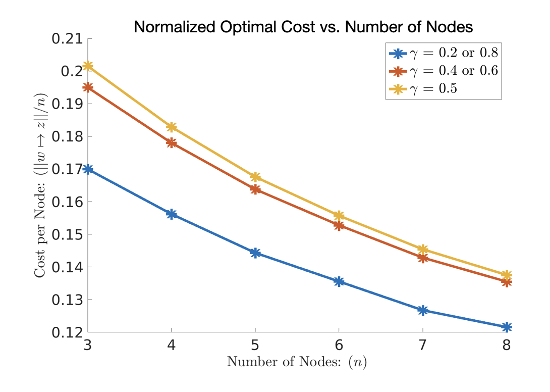
Figure 1: Cost per node ($\frac{1}{n}||\bm{w}\mapsto\bm{z}||$) for the $\mathcal{H}_{2}$ optimal controller for the consensus problem with controller communication delays as a function of the network size $n$.

VII Conclusion

Relative measurement structures are common in distributed systems, but previously this structural requirement has not been considered as a design constraint. We provided a characterization of relative measurement structures as such a design constraint, and this allowed us to convert the optimal controller design problem to an equivalent convex program. This formulation may aid in the understanding of fundamental properties of relative measurement systems such as best achievable performance. The ability to convert our formulation to a model-matching problem for the consensus example further suggests this is the case. Indeed, this form may admit analytic solutions that could provide insight to system properties. Ongoing work is focused on extensions of these results to allow for more general relative measurements, e.g. differences of outputs rather than differences of states. Another interesting line of questioning is to characterize which network control structures will allow for a convex formulation with our methodology - specifically focusing on the cases of decoupled subsystem dynamics or system dynamics that depend only on relative states.

Appendix

Proof of Theorem 1

We utilize the following lemmas to prove this result. The proofs of these lemmas are straightforward and thus are omitted for the sake of space.

Lemma 2.

Any relative linear map $f(x)=Fx$ on $\mathbb{R}^{n}$ can be written as

$$f(x)=\sum_{i=1}^{n-1}g_{i}(x_{i}-x_{i+1}),$$ (52)

for some set of vectors $\{g_{i}\}.$

Lemma 3.

If $\mathcal{A}_{\rm meas.}$ computed from (5) is corresponds to a connected graph, then there exists an invertible matrix $T$ for which

$$(TC_{2})x=\underbrace{\left[\begin{array}[]{ccccc}1&-1\\ &1&-1\\ &&\ddots&\ddots\\ &&&1&-1\end{array}\right]}_{=:M}\left[\begin{array}[]{c}x_{1}\\ x_{2}\\ \vdots\\ x_{n}\end{array}\right]=\left[\begin{array}[]{c}x_{1}-x_{2}\\ x_{2}-x_{3}\\ \vdots\\ x_{n-1}-x_{n}\end{array}\right].$$ (53)

Lemma 4.

Consider two LTI systems ${\bm{K}}$ and ${\bm{R}}$ with Markov parameters $\{D_{K},C_{K}B_{K},C_{K}A_{K}B_{K},...\}$ and $\{D_{R},C_{R}B_{R},C_{R}A_{R}B_{R},...\}$, respectively. For a static matrix $C_{2},$ the relation

$${\bm{K}}C_{2}={\bm{R}}$$ (54)

holds if and only if the matrix equalities

$$D_{K}C_{2}=D_{R}, C_{K}A_{K}^{i}B_{K}C_{2}=C_{R}A_{R}^{i}B_{R},~{}i\geq 0$$ (55)

hold.

We first consider the case of connected $\mathcal{A}_{\rm meas.}$ By Lemma 3, to show that there is a solution ${\bm{K}}$ to ${\bm{K}}C_{2}={\bm{R}}$ if and only if ${\bm{R}}$ is relative, it is sufficient to show that there exists a solution $\tilde{\bm{K}}$ to

$$\tilde{\bm{K}}M={\bm{R}}$$ (56)

if and only if ${\bm{R}},$ since ${\bm{K}}C_{2}={\bm{R}}$ can always be written as ${\bm{K}}T^{-1}M={\bm{R}}$ for some $T.$ By Lemma 4, to prove this, it is sufficient to show that there is always a solution $G$ to the matrix equation

$$GM=F$$ (57)

if and only if $F$ is a relative matrix. For the first direction of this implication, note that the vector of all ones will be in the null space of $M$, so that (57) could only hold if this same vector is in the null space of $F.$ It is straightforward to show that this is the case only if $F$ is relative. For the converse direction, note that (57) holds only if $GMx=Fx$ for all $x\in\mathbb{R}^{n}.$ By Lemma 2, $Fx=\sum_{i=1}^{n-1}g_{i}(x_{i}-x_{i+1})$ for some vectors $\{g_{i}\}$ so that a solution $G$ of (57) exists and is given by $G=\left[\begin{array}[]{cccc}g_{1}&g_{2}&\cdots&g_{n-1}\end{array}\right]$.

We next consider the case that $A_{\rm meas.}$ corresponds to a graph with $N>1$ connected components. In this case, assuming ${\bm{R}}$ satisfies (16), we are searching for a ${\bm{K}}$ that satisfies

$${\bm{K}}C_{2}{\bm{x}}=\sum_{i=1}^{N}{\bm{R}}^{(i)}{\bm{x}}^{(i)}$$ (58)

for all ${\bm{x}}.$ The left hand side of (58) as

$$\left[\begin{array}[]{cccc}{\bm{K}}_{1}&{\bm{K}}_{2}&\cdots&{\bm{K}}_{N}\end{array}\right]\left[\begin{array}[]{cccc}M^{(1)}\\ &M^{(2)}\\ &&\ddots\\ &&&M^{(N)}\end{array}\right]\left[\begin{array}[]{c}{\bm{x}}^{(1)}\\ {\bm{x}}^{(2)}\\ \vdots\\ {\bm{x}}^{(N)}\end{array}\right]$$

where each $M^{(i)}$ is of the same form as $M$ introduced in (53) of appropriate dimensions and ${\bm{K}}$ is partitioned into block columns accordingly. Then this problem reduces to solving $N$ problems of the form ${\bm{K}}_{i}M^{(i)}=R^{(i)}$, which follows from the results in the connected graph setting.

References

- [1] M. Rotkowitz and S. Lall, “A characterization of convex problems in decentralized control,” IEEE transactions on Automatic Control, vol. 50, no. 12, pp. 1984–1996, 2005.
- [2] B. Bamieh and P. G. Voulgaris, “A convex characterization of distributed control problems in spatially invariant systems with communication constraints,” Systems & control letters, vol. 54, no. 6, pp. 575–583, 2005.
- [3] R. S. Smith and F. Y. Hadaegh, “Control of deep-space formation-flying spacecraft; relative sensing and switched information,” Journal of Guidance, Control, and Dynamics, vol. 28, no. 1, pp. 106–114, 2005.
- [4] M. R. Jovanovic and B. Bamieh, “On the ill-posedness of certain vehicular platoon control problems,” IEEE Transactions on Automatic Control, vol. 50, no. 9, pp. 1307–1321, 2005.
- [5] E. Tegling, B. Bamieh, and D. F. Gayme, “The price of synchrony: Evaluating the resistive losses in synchronizing power networks,” IEEE Transactions on Control of Network Systems, vol. 2, no. 3, pp. 254–266, 2015.
- [6] A. Karimian and R. Tron, “Bearing-only consensus and formation control under directed topologies,” in 2020 American Control Conference (ACC), pp. 3503–3510, 2020.
- [7] M. H. Trinh, S. Zhao, Z. Sun, D. Zelazo, B. D. Anderson, and H.-S. Ahn, “Bearing-based formation control of a group of agents with leader-first follower structure,” IEEE Transactions on Automatic Control, vol. 64, no. 2, pp. 598–613, 2018.
- [8] F. Bullo, Lectures on network systems, vol. 1. Kindle Direct Publishing Seattle, DC, USA, 2020.
- [9] Q. Song, F. Liu, J. Cao, A. V. Vasilakos, and Y. Tang, “Leader-following synchronization of coupled homogeneous and heterogeneous harmonic oscillators based on relative position measurements,” IEEE Transactions on Control of Network Systems, vol. 6, no. 1, pp. 13–23, 2019.
- [10] E. Tegling and H. Sandberg, “On the coherence of large-scale networks with distributed pi and pd control,” IEEE control systems letters, vol. 1, no. 1, pp. 170–175, 2017.
- [11] D. Zelazo and M. Mesbahi, “Graph-theoretic analysis and synthesis of relative sensing networks,” IEEE Transactions on Automatic Control, vol. 56, no. 5, pp. 971–982, 2010.
- [12] M. Mesbahi and M. Egerstedt, Graph theoretic methods in multiagent networks. Princeton University Press, 2010.
- [13] H. G. Oral and D. F. Gayme, “Disorder in large-scale networks with uni-directional feedback,” in 2019 American Control Conference (ACC), pp. 3394–3401, IEEE, 2019.
- [14] E. Jensen and B. Bamieh, “On the gap between system level synthesis and structured controller design: the case of relative feedback,” in 2020 American Control Conference (ACC), pp. 4594–4599, IEEE, 2020.
- [15] Y.-S. Wang, N. Matni, and J. C. Doyle, “A system-level approach to controller synthesis,” IEEE Transactions on Automatic Control, vol. 64, no. 10, pp. 4079–4093, 2019.
- [16] D. Youla, H. Jabr, and J. Bongiorno, “Modern wiener-hopf design of optimal controllers–part ii: The multivariable case,” IEEE Transactions on Automatic Control, vol. 21, no. 3, pp. 319–338, 1976.
- [17] B. A. Francis, A course in H control theory. Springer, 1987.
- [18] B. Bamieh, F. Paganini, and M. A. Dahleh, “Distributed control of spatially invariant systems,” IEEE Transactions on automatic control, vol. 47, no. 7, pp. 1091–1107, 2002.