A lower bound for the genus of a knot using the Links-Gould invariant

Abstract.

The Links-Gould invariant of links $LG^{2,1}$ is a two-variable generalization of the Alexander-Conway polynomial. Using representation theory of $U_{q}\mathfrak{gl}(2|1)$, we prove that the degree of the Links-Gould polynomial provides a lower bound on the Seifert genus of any knot, therefore improving the bound known as the Seifert inequality in the case of the Alexander invariant.

One practical consequence of this new genus bound is a straightforward proof of the fact that the Kinoshita-Terasaka and Conway knots have genus greater or equal to 2.

1. Introduction

The Links-Gould invariants of oriented links $LG^{m,n}(L,t_{0},t_{1})$ are obtained by the Reshetikhin-Turaev construction applied to Hopf superalgebras $U_{q}\mathfrak{gl}(m|n)$. We will specifically study $U_{q}\mathfrak{gl}(2|1)$ and we shall denote by $LG$ the associated invariant $LG^{2,1}$.

For any oriented link $L$, $LG(L,t_{0},t_{1})$ is a two-variable Laurent polynomial in variables $t_{0}$ and $t_{1}$. It is known to be a generalization of the Alexander-Conway polynomial $\Delta_{L}(t_{0})$ in at least two different ways (see [2, 10, 11]):

$$LG(L,t_{0},-t_{0}^{-1})=\Delta_{L}(t_{0}^{2})\text{ ;}$$

$$LG(L,t_{0},t_{0}^{-1})=\Delta_{L}(t_{0})^{2}.$$

Therefore, using the Seifert inequality for the Alexander polynomial $\Delta_{K}$ of a knot $K$, the minimal genus $g(K)$ among all possible Seifert surfaces for $K$ satisfies the following inequality:

(1.1) $$deg(LG(K,t_{0},t_{0}^{-1}))\leq 4g(K)$$

where the degree $deg(LG(K,t_{0},t_{0}^{-1}))$ of Laurent polynomial $LG(K,t_{0},t_{0}^{-1})$ is the difference between the degree of the monomial of highest degree and that of the monomial of lowest degree.

That is why, defining $deg(t_{0}^{a}t_{1}^{b})$ to be $a-b$, one can wonder whether the following stronger inequality holds:

(1.2) $$deg(LG(K,t_{0},t_{1}))\leq 4g(K).$$

This is one of many features of the Links-Gould invariant, proven or conjectured, that illustrate the fact that this quantum invariant has deep topological meaning (see in particular [7, 9]). In general, it is hard to deduce precise topological properties on a knot or link from the value quantum invariants take on that link. For instance, no genus bound is known for the Jones polynomial.

In this paper we prove inequality (1.2) that had been conjectured in [9]. In particular,  (1.1) shows that the bound obtained that way systematically improves the classical lower bound for the genus of a knot given by the Alexander invariant.

Theorem 1.1.

Setting $deg(\sum\limits_{i,j}a_{i,j}t_{0}^{i}t_{1}^{j})=max\{{i-j\leavevmode\nobreak\ |\leavevmode\nobreak\ a_{i,j}\neq 0)\}}-min\{{i-j\leavevmode\nobreak\ |\leavevmode\nobreak\ a_{i,j}\neq 0)\}}$, for any knot $K$:

$$deg(LG(K,t_{0},t_{1}))\leq 4g(K).$$

As it is explained in [9], Proposition 1.13, a consequence of this inequality and of [14] is the following.

Corollary 1.2.

If $K$ is an alternating knot, then the inequality in Theorem 1.1 is an equality.

One example where the bound given by Theorem 1.1 improves the usual bound obtained by computing the Alexander polynomial is if you compute $LG$ on the Kinoshita-Terasaka and Conway pair of mutant knots. The new genus bound proves that both these knots, that have the same $LG$, are of genus greater or equal to 2. This is significant since both the Alexander invariant and the Levine-Tristram signature fail to detect genus for the pair.

Organization of the paper

Theorem 1.1 is proved in Section 3. The genus bound is seen as a consequence of a "factorization" of the diagram of a knot $K$ through the Reshetikhin-Turaev functor in a way that is controlled by the genus of $K$. For that we use the so called bottom tangle presentation of a Seifert surface of a knot [5]. This construction follows the spirit of recent work by López Neumann and Van der Veen (see [12]).

One crucial step to use that factorization is a representation-theoretic lemma obtained in Section 2. The Links-Gould invariant is associated to a family of highest weight supermodules over $U_{q}\mathfrak{gl}(2|1)$. Equivalently, it can be obtained from a family of modules $(V_{\alpha})$ over the bosonization $U_{q}\mathfrak{gl}(2|1)^{\sigma}$ of superalgebra $U_{q}\mathfrak{gl}(2|1)$. In Theorem 2.12, we prove that the tensor product representation $V_{\alpha}\otimes V_{\alpha}^{\ast}$ does not depend on parameter $\alpha$. For that purpose we provide an explicit change of basis between $U_{q}\mathfrak{gl}(2|1)^{\sigma}$-modules. We also need to understand the dual action of $U_{q}\mathfrak{gl}(2|1)^{\sigma}$ on $(V_{\alpha}\otimes V_{\alpha}^{\ast})^{\ast}$ which we do at the end of Section 2.

Some topological consequences of this new genus bound are presented in Section 4.

Conventions

All along the paper, we stick to the conventions David De Wit uses in his Ph.D. dissertation (see [1]). Specifically, $LG$ is a two-variable Laurent polynomial in variables $t_{0}$ and $t_{1}$. But it can also be expressed using variables $q$ and $q^{\alpha}$ with the following dictionary:

$$t_{0}^{1/2}=q^{-\alpha}\text{, }t_{1}^{1/2}=q^{\alpha}q.$$

In this setting, the degree defined in $\mathbb{Z}[t_{0}^{\pm 1},t_{1}^{\pm 1}]$ by $deg(t_{0}^{a}t_{1}^{b})=a-b$ is none other than the degree with respect to variable $q^{\alpha}$ in $\mathbb{Z}(q)[q^{\alpha},q^{-\alpha}]$ with:

$$deg(q^{2n\alpha})=n.$$

This will be important for our upcoming computations.

Acknowledgments

The first author would like to thank BIMSA for the hospitality during his stay in Beijing in September of 2023, when this project was initiated and carried out. The authors would also like to thank Bertrand Patureau-Mirand very warmly for his insightful advice all through the process, as well as David Cimasoni and Jon Links for their valuable remarks.

2. Representations of Hopf superalgebra $U_{q}\mathfrak{gl}(2|1)$

But let us first introduce the objects at hand.

2.1. Generators and relations for Hopf superalgebra $U_{q}\mathfrak{gl}(2|1)$

2.1.1. Generators

Superalgebra $U_{q}\mathfrak{gl}(2|1)$ is a $\mathbb{C}$-superalgebra defined by the following seven elementary generators:

• Cartan generators $q^{E_{1}^{1}}$, $q^{E_{2}^{2}}$ and $q^{E_{3}^{3}}$;

• Raising generators $E_{2}^{1}$ and $E_{3}^{2}$;

• Lowering generators $E_{1}^{2}$ and $E_{2}^{3}$.

Elements $q^{E_{i}^{i}}$ are chosen to be invertible and we refer to their inverses as $q^{-E_{i}^{i}}$. We also denote by $q^{\frac{1}{2}E_{i}^{i}}$ some choice of a square root for $q^{E_{i}^{i}}$.

In addition to the 7 generators, we will use two other elements defined in terms of them:

• $E_{3}^{1}=E_{2}^{1}E_{3}^{2}-q^{-1}E_{3}^{2}E_{2}^{1}$;

• $E_{1}^{3}=E_{2}^{3}E_{1}^{2}-qE_{1}^{2}E_{2}^{3}$.

Remark 2.1.

This choice of variables is coherent with [18] up to the fact that what Zhang calls $K_{a}$ corresponds to what we denote $q^{(-1)^{|a|}E_{a}^{a}}$ in the following paragraph.

2.1.2. $\mathbb{Z}/2\mathbb{Z}$-grading

We define a $\mathbb{Z}/2\mathbb{Z}$-grading on $U_{q}\mathfrak{gl}(2|1)$ by fixing $q^{E_{1}^{1}}$, $q^{E_{2}^{2}}$, $q^{E_{3}^{3}}$, $E_{2}^{1}$ and $E_{1}^{2}$ to be even while declaring the two last generators $E_{3}^{2}$ and $E_{2}^{3}$ odd. We can extend that grading to the rest of the algebra. Setting $[x]$ the degree of homogeneous $x$ ($[x]=0$ if $x$ is even and $[x]=1$ is $a$ is odd), the product of homogeneous $x$, $y$ $\in U_{q}\mathfrak{gl}(2|1)$ has degree:

$$[xy]=[x]+[y]\text{ modulo 2.}$$

In particular, $E_{3}^{1}$ and $E_{1}^{3}$ are odd.

2.1.3. Relations

Definition 2.2.

Whenever it makes sense, we will use the following q-bracket notation:

$$[X]_{q}=\frac{q^{X}-q^{-X}}{q-q^{-1}}.$$

That being said, the relations defining superalgebra $U_{q}\mathfrak{gl}(2|1)$ are:

• The Cartan generators $q^{E_{1}^{1}}$, $q^{E_{2}^{2}}$, $q^{E_{3}^{3}}$ all commute;

• The raising and lowering generators commute with the Cartan genarators as follows:

  $$q^{(-1)^{|a|}E^{a}_{a}}E^{b}_{b\pm 1}q^{-(-1)^{|a|}E^{a}_{a}}=q^{(-1)^{|a|}(\delta^{a}_{b}-\delta^{a}_{b\pm 1})}E^{b}_{b\pm 1},$$

  $\text{where }|1|=|2|=0\text{, }|3|=1\text{ and }\delta^{i}_{j}=1\text{ if and only if }i=j;$

• $(E_{2}^{3})^{2}=(E_{3}^{2})^{2}=0$ (the squares of odd generators are zero);

• $E^{1}_{2}$ commutes with $E_{2}^{3}$ while $E_{1}^{2}$ commutes with $E_{3}^{2}$;

• The non Cartan generators also satisfy the following interchange rules:

  $$E_{2}^{1}E_{1}^{2}=[E_{1}^{1}-E_{2}^{2}]_{q}+E_{1}^{2}E_{2}^{1},$$

  $$E_{3}^{2}E_{2}^{3}=[E_{2}^{2}+E_{3}^{3}]_{q}-E_{2}^{3}E_{3}^{2}.$$

The Serre relations can be written in terms of generators, but are more easily understood when expressed using $E^{3}_{1}$ and $E^{1}_{3}$:

$$E_{2}^{1}E_{3}^{1}-qE_{3}^{1}E_{2}^{1}=0;$$

$$E_{1}^{3}E_{1}^{2}-q^{-1}E_{1}^{2}E_{1}^{3}=0.$$

Other interesting relations can be deduced from the defining ones. They are all summed up in [1], Sections 4.2.3 and 4.2.4.

2.2. A Hopf superalgebra structure on $U_{q}\mathfrak{gl}(2|1)$

Superalgebra $U_{q}\mathfrak{gl}(2|1)$ is equipped with a coproduct $\Delta$, a co-unit $\epsilon$ and an antipode $S$, turning it into a Hopf superalgebra.

2.2.1. Coproduct

Coproduct $\Delta:U_{q}\mathfrak{gl}(2|1)\rightarrow U_{q}\mathfrak{gl}(2|1)\otimes U_{q}\mathfrak{gl}(2|1)$ is an algebra homomorphism defined by $\Delta(xy)=\Delta(x)\Delta(y)\text{ for any }x,y\in U_{q}\mathfrak{gl}(2|1)\text{, by }$ $\Delta(1)=1\otimes 1$ and by:

$$\text{ for any }i\text{, }\Delta(q^{E_{i}^{i}})=q^{E_{i}^{i}}\otimes q^{E_{i}^{i}};$$

$$\Delta(E_{2}^{1})=E_{2}^{1}\otimes q^{-\frac{1}{2}(E_{1}^{1}-E_{2}^{2})}+q^{\frac{1}{2}(E_{1}^{1}-E_{2}^{2})}\otimes E_{2}^{1};$$

$$\Delta(E_{1}^{2})=E_{1}^{2}\otimes q^{-\frac{1}{2}(E_{1}^{1}-E_{2}^{2})}+q^{\frac{1}{2}(E_{1}^{1}-E_{2}^{2})}\otimes E_{1}^{2};$$

$$\Delta(E_{3}^{2})=E_{3}^{2}\otimes q^{-\frac{1}{2}(E_{2}^{2}+E_{3}^{3})}+q^{\frac{1}{2}(E_{2}^{2}+E_{3}^{3})}\otimes E_{3}^{2};$$

$$\Delta(E_{2}^{3})=E_{2}^{3}\otimes q^{-\frac{1}{2}(E_{2}^{2}+E_{3}^{3})}+q^{\frac{1}{2}(E_{2}^{2}+E_{3}^{3})}\otimes E_{2}^{3}.$$

Remark 2.3.

Observe that coproduct $\Delta$ preserves grading: for any $x\in U_{q}\mathfrak{gl}(2|1)$, $[\Delta(x)]=[x]$.

It will be necessary to know the expression for coproducts $\Delta(E_{1}^{3})$ and $\Delta(E_{3}^{1})$. They have been computed in [1], Section 4.5.3:

• $\Delta(E_{1}^{3})=E_{1}^{3}\otimes q^{-\frac{1}{2}(E_{1}^{1}+E_{3}^{3})}+q^{\frac{1}{2}(E_{1}^{1}+E_{3}^{3})}E_{1}^{3}-(q-q^{-1})q^{\frac{1}{2}(E_{1}^{1}-E_{2}^{2})}E_{2}^{3}\otimes E_{1}^{2}q^{-\frac{1}{2}(E_{2}^{2}+E_{3}^{3})}$;

• $\Delta(E_{3}^{1})=E_{3}^{1}\otimes q^{-\frac{1}{2}(E_{1}^{1}+E_{3}^{3})}+q^{\frac{1}{2}(E_{1}^{1}+E_{3}^{3})}E_{3}^{1}+(q-q^{-1})q^{\frac{1}{2}(E_{2}^{2}+E_{3}^{3})}E_{2}^{1}\otimes E_{3}^{2}q^{-\frac{1}{2}(E_{1}^{1}-E_{2}^{2})}$.

2.2.2. Co-unit

Co-unit $\epsilon:U_{q}\mathfrak{gl}(2|1)\rightarrow\mathbb{C}$ is a algebra homomorphism satisfying:

$$\epsilon(q^{E_{1}^{1}})=\epsilon(q^{E_{2}^{2}})=\epsilon(q^{E_{3}^{3}})=\epsilon(1)=1;$$

$$\epsilon(E_{2}^{1})=\epsilon(E_{1}^{2})=\epsilon(E_{3}^{2})=\epsilon(E_{2}^{3})=0.$$

2.2.3. Antipode

Antipode $S:U_{q}\mathfrak{gl}(2|1)\rightarrow U_{q}\mathfrak{gl}(2|1)$ is a graded algebra antihomomorphism. It satisfies $S(1)=1$ and $S(xy)=(-1)^{[x][y]}S(y)S(x)$ for any $x,y\in U_{q}\mathfrak{gl}(2|1)$. Also:

$$S(q^{E_{i}^{i}})=q^{-E_{i}^{i}}\text{ for }i=1,2,3;$$

$$S(E_{2}^{1})=-q^{-1}E_{2}^{1}\text{ and }S(E_{1}^{2})=-qE_{1}^{2};$$

$$S(E_{3}^{2})=-E_{3}^{2}\text{ and }S(E_{2}^{3})=-E_{2}^{3}.$$

Superalgebra $U_{q}\mathfrak{gl}(2|1)$ equipped with $\Delta,\epsilon,S$ satisfies the standard axioms for Hopf superalgebras, see [17].

2.3. Highest weight representations on $U_{q}\mathfrak{gl}(2|1)$

A super vector space $V=V^{even}\oplus V^{odd}$ is a representation of $U_{q}\mathfrak{gl}(2|1)$ when $U_{q}\mathfrak{gl}(2|1)$ acts on $V$ from the left in a way that preserves the grading. In other words, for $a\in U_{q}\mathfrak{gl}(2|1)$ and $x$ an homogeneous element in $V$, we have $[a.x]=[a].[x]$ (where $[x]=0$ if $x\in V^{even}$ and $[x]=1$ if $x\in V^{odd}$).

We introduce a family of $4$-dimensional representations of $U_{q}\mathfrak{gl}(2|1)$ that will help us define the Links-Gould invariant. It is a family of irreducible typical highest weight representations $(V_{\alpha})$, $\alpha\neq-1,0$.

Definition 2.4.

For any $\alpha\in\mathbb{C}\setminus\{{-1,0\}}$, $V_{\alpha}$ is a $(2|2)$ super vector space spanned by $e_{1},e_{2},e_{3}\text{ and }e_{4}$ where $[e_{1}]=[e_{4}]=0$ while $[e_{2}]=[e_{3}]=1$.

The matrices representing the action of the generators of $U_{q}\mathfrak{gl}(2|1)$ on $V_{\alpha}$ are as follows:

$$\pi_{\alpha}(q^{E_{1}^{1}})=\begin{pmatrix}1&0&0&0\\ 0&1&0&0\\ 0&0&q^{-1}&0\\ 0&0&0&q^{-1}\end{pmatrix};\text{ }\pi_{\alpha}(q^{E_{2}^{2}})=\begin{pmatrix}1&0&0&0\\ 0&q^{-1}&0&0\\ 0&0&1&0\\ 0&0&0&q^{-1}\end{pmatrix};\text{ }\pi_{\alpha}(q^{E_{3}^{3}})=\begin{pmatrix}q^{\alpha}&0&0&0\\ 0&q^{\alpha+1}&0&0\\ 0&0&q^{\alpha+1}&0\\ 0&0&0&q^{\alpha+2}\end{pmatrix};$$

$$\pi_{\alpha}(E_{2}^{1})=\begin{pmatrix}0&0&0&0\\ 0&0&-1&0\\ 0&0&0&0\\ 0&0&0&0\end{pmatrix};\text{ }\pi_{\alpha}(E_{1}^{2})=\begin{pmatrix}0&0&0&0\\ 0&0&0&0\\ 0&-1&0&0\\ 0&0&0&0\end{pmatrix};\text{ }\pi_{\alpha}(E_{3}^{2})=\begin{pmatrix}0&1&0&0\\ 0&0&0&0\\ 0&0&0&1\\ 0&0&0&0\end{pmatrix};$$

$$\pi_{\alpha}(E_{2}^{3})=\begin{pmatrix}0&0&0&0\\ [\alpha]_{q}&0&0&0\\ 0&0&0&0\\ 0&0&[\alpha+1]_{q}&0\end{pmatrix};\text{ }\pi_{\alpha}(E_{3}^{1})=\begin{pmatrix}0&0&q^{-1}&0\\ 0&0&0&-1\\ 0&0&0&0\\ 0&0&0&0\end{pmatrix};\text{ }\pi_{\alpha}(E_{1}^{3})=\begin{pmatrix}0&0&0&0\\ 0&0&0&0\\ q[\alpha]_{q}&0&0&0\\ 0&-[\alpha+1]_{q}&0&0\end{pmatrix},$$

where $[x]_{q}$ stands for $\frac{q^{x}-q^{-x}}{q-q^{-1}}$.

This family of representations is a one-parameter family of highest weight irreducible representations of $U_{q}\mathfrak{gl}(2|1)$ (see [4]).

Remark 2.5.

Matrices in Definition 2.4 are usual matrices and not super-matrices.

Remark 2.6.

In order to write these matrices we modified the basis used in [1]:

• $|1\rangle$ is replaced by $\frac{[\alpha]_{q}^{1/2}}{[\alpha+1]_{q}^{1/2}}|1\rangle=e_{1}$;

• $|2\rangle$ is replaced by $\frac{1}{[\alpha+1]_{q}^{1/2}}|2\rangle=e_{2}$;

• $|3\rangle$ is replaced by $\frac{1}{[\alpha+1]_{q}^{1/2}}|3\rangle=e_{3}$;

• $|4\rangle$ is replaced by $\frac{1}{[\alpha+1]_{q}}|4\rangle=e_{4}$.

Remark 2.7.

One can verify that the following relation holds. It is a useful tool for computations in this context:

$$[\alpha+1]_{q}q^{\alpha}-[\alpha]_{q}q^{\alpha+1}=1.$$

2.4. Bosonization of Hopf superalgebra $U_{q}\mathfrak{gl}(2|1)$

In order to make computations a bit more straightforward, we will not in practice use Hopf superalgebra $U_{q}\mathfrak{gl}(2|1)$, but its non super counterpart $U_{q}\mathfrak{gl}(2|1)^{\sigma}$. This transformation, known as bosonization, is due to Majid, see [13].

Theorem 2.8.

Set $(H,\Delta,\epsilon,S)$ a Hopf superalgebra. One can define an ordinary Hopf algebra $H^{\sigma}$ as follows. As an algebra, $H^{\sigma}$ is an extension of $H$ by adjoining an element ${\sigma}$ subject to the following commutation relations:

$$\forall x\in H\text{ homogeneous, }\sigma x=(-1)^{[x]}x\sigma.$$

The coproduct $\Delta^{\sigma}$ on $H^{\sigma}$ is given by $\Delta^{\sigma}(\sigma)=\sigma\otimes\sigma$ and

$$\forall x\in H\text{, }\Delta^{\sigma}(x)=\displaystyle\sum_{i}x_{i}\sigma^{[y_{i}]}\otimes y_{i}\text{ where }\Delta(x)=\displaystyle\sum_{i}x_{i}\otimes y_{i}.$$

The counit $\epsilon^{\sigma}$ satisfies $\epsilon^{\sigma}(\sigma)=1$ and $\epsilon^{\sigma}(x)=\epsilon(x)$ otherwise.

The antipode $S^{\sigma}$ is given by $S^{\sigma}(\sigma)=\sigma$ and

$$S^{\sigma}(x)=\sigma^{[x]}S(x)\text{ }\forall x\in H\text{ homogeneous.}$$

Note that $S$ is a graded algebra antihomomorphism and therefore $S^{\sigma}$ is an ordinary algebra antihomomorphism.

Theorem 2.9.

For any superalgebra $H$, the category of super $H$-modules (where arrows are even morphisms) is equivalent to the category of $H^{\sigma}$-modules.

This is essentially due to the fact that if you consider a super-representation $V=V_{even}\oplus V_{odd}$ of $H$, then you get a representation of $H^{\sigma}$ by setting $\sigma_{V}=\text{Id}_{V_{even}}\oplus-\text{Id}_{V_{odd}}$. Reciprocally, since $\sigma^{2}=1$, every $H^{\sigma}$-module inherits a natural $\mathbb{Z}/2\mathbb{Z}$ grading: any $V$ splits into $V=V_{even}\oplus V_{odd}$ where $V_{even}=\ker(\sigma-1)$ and $V_{odd}=\ker(\sigma+1)$.

That is why in the following we will consider Hopf algebra $U_{q}\mathfrak{gl}(2|1)^{\sigma}$ rather than Hopf superalgebra $U_{q}\mathfrak{gl}(2|1)$. They tell the same story representation-wise.

2.5. Dual representations $V_{\alpha}^{\ast}$

We use $U_{q}\mathfrak{gl}(2|1)^{\sigma}$’s Hopf algebra structure to build the family of dual representations $(V_{\alpha}^{\ast})$. Setting $\pi_{\alpha}^{\ast}$ the dual representation of $\pi_{{\alpha}}$, we can write:

$$\forall f\in V_{\alpha}^{\ast},\forall x\in U_{q}\mathfrak{gl}(2|1)^{\sigma}\text{ : }\pi_{\alpha}^{\ast}(x)(f)=f\circ\pi_{{\alpha}}(S^{\sigma}(x))\in V_{\alpha}^{\ast}.$$

Computing the latter in basis $(e_{1}^{\ast},e_{2}^{\ast},e_{3}^{\ast},e_{4}^{\ast})$, we obtain for any $x\in U_{q}\mathfrak{gl}(2|1)^{\sigma}$ that:

$$\pi_{\alpha}^{\ast}(x)(e_{i}^{\ast})=\sum\limits_{j=1}^{4}(\pi_{\alpha}^{\ast}(x)(e_{i}^{\ast})(e_{j}))e_{j}^{\ast}.$$

This means that if $A$ is the matrix for $\pi_{{\alpha}}(S^{\sigma}(x))$ in basis $(e_{1},e_{2},e_{3},e_{4})$, then $A^{T}$ is the matrix for $\pi_{\alpha}^{\ast}(x)$ in basis $(e_{1}^{\ast},e_{2}^{\ast},e_{3}^{\ast},e_{4}^{\ast})$.

From that we deduce the matrices representing left multiplication by generators of $U_{q}\mathfrak{gl}(2|1)^{\sigma}$ on $V_{\alpha}^{\ast}$ :

$$\pi_{\alpha}^{\ast}(q^{E_{1}^{1}})=\begin{pmatrix}1&0&0&0\\ 0&1&0&0\\ 0&0&q&0\\ 0&0&0&q\end{pmatrix};\text{ }\pi_{\alpha}^{\ast}(q^{E_{2}^{2}})=\begin{pmatrix}1&0&0&0\\ 0&q&0&0\\ 0&0&1&0\\ 0&0&0&q\end{pmatrix};\text{ }\pi_{\alpha}^{\ast}(q^{E_{3}^{3}})=\begin{pmatrix}q^{-\alpha}&0&0&0\\ 0&q^{-\alpha-1}&0&0\\ 0&0&q^{-\alpha-1}&0\\ 0&0&0&q^{-\alpha-2}\end{pmatrix};$$

$\pi_{\alpha}^{\ast}(E_{2}^{1})=\begin{pmatrix}0&0&0&0\\ 0&0&0&0\\ 0&q^{-1}&0&0\\ 0&0&0&0\end{pmatrix};\text{ }\pi_{\alpha}^{\ast}(E_{1}^{2})=\begin{pmatrix}0&0&0&0\\ 0&0&q&0\\ 0&0&0&0\\ 0&0&0&0\end{pmatrix};\text{ }\pi_{\alpha}^{\ast}(E_{3}^{2})=\begin{pmatrix}0&0&0&0\\ -1&0&0&0\\ 0&0&0&0\\ 0&0&1&0\end{pmatrix};\text{ }\pi_{\alpha}^{\ast}(E_{2}^{3})=\begin{pmatrix}0&[\alpha]_{q}&0&0\\ 0&0&0&0\\ 0&0&0&-[\alpha+1]_{q}\\ 0&0&0&0\end{pmatrix};$

$$\pi_{\alpha}^{\ast}(E_{3}^{1})=\begin{pmatrix}0&0&0&0\\ 0&0&0&0\\ -q^{-1}&0&0&0\\ 0&-q^{-2}&0&0\end{pmatrix};\text{ }\pi_{\alpha}^{\ast}(E_{1}^{3})=\begin{pmatrix}0&0&q[\alpha]_{q}&0\\ 0&0&0&q^{2}[\alpha+1]_{q}\\ 0&0&0&0\\ 0&0&0&0\end{pmatrix};\text{ }\pi_{\alpha}^{\ast}(\sigma)=\begin{pmatrix}1&0&0&0\\ 0&-1&0&0\\ 0&0&-1&0\\ 0&0&0&1\end{pmatrix}.$$

2.6. Tensor representations $V_{\alpha}\otimes V_{\alpha}^{\ast}$

Now we will compute the tensor product $V_{\alpha}\otimes V_{\alpha}^{\ast}$ of the representations we studied in the two previous paragraphs. To do so we need to build the tensor product of two representations in the context of Hopf algebras.

Definition 2.10.

If the actions of $U_{q}\mathfrak{gl}(2|1)^{\sigma}$ on two vector spaces $V$ and $W$ are denoted by $\rho_{V}$ and $\rho_{W}$, then $U_{q}\mathfrak{gl}(2|1)^{\sigma}$ acts on $V\otimes W$ through co-multiplication. Indeed, for any $a\in U_{q}\mathfrak{gl}(2|1)^{\sigma}$

$$\rho_{V\otimes W}(a)=\rho_{V}\otimes\rho_{W}(\Delta^{\sigma}(a)),$$

where the action of $U_{q}\mathfrak{gl}(2|1)^{\sigma}\otimes U_{q}\mathfrak{gl}(2|1)^{\sigma}$ on $V\otimes W$ is defined naturally for $X,Y\in U_{q}\mathfrak{gl}(2|1)^{\sigma}$, $v\in V$ and $w\in W$ as follows:

$$(X\otimes Y)(v\otimes w)=(X.v\otimes Y.w).$$

With that we can compute the action of $U_{q}\mathfrak{gl}(2|1)^{\sigma}$ on $V_{\alpha}\otimes V_{\alpha}^{\ast}$. We write the 16x16 matrices representing left multiplication on $V_{\alpha}\otimes V_{\alpha}^{\ast}$ in basis $(e_{1}\otimes e_{1}^{\ast},e_{1}\otimes e_{2}^{\ast},e_{1}\otimes e_{3}^{\ast},e_{1}\otimes e_{4}^{\ast},e_{2}\otimes e_{1}^{\ast},e_{2}\otimes e_{2}^{\ast},\ldots)$. The representation is denoted $\Pi_{\alpha}$.

$\Pi_{\alpha}(q^{E_{1}^{1}})$ is a diagonal matrix with entries $(1,1,q,q,1,1,q,q,q^{-1},q^{-1},1,1,q^{-1},q^{-1},1,1)$ ;

$\Pi_{\alpha}(q^{E_{2}^{2}})$ is a diagonal matrix with entries $(1,q,1,q,q^{-1},1,q^{-1},1,1,q,1,q,q^{-1},1,q^{-1},1)$ ;

$\Pi_{\alpha}(q^{E_{3}^{3}})$ is a diagonal matrix with entries $(1,q^{-1},q^{-1},q^{-2},q,1,1,q^{-1},q,1,1,q^{-1},q^{2},q,q,1)$ ;

$\Pi_{\alpha}(\sigma)$ is a diagonal matrix with entries $(1,-1,-1,1,-1,1,1,-1,-1,1,1,-1,1,-1,-1,1)$ ;

$$\Pi_{\alpha}(E_{2}^{1})=\left(\begin{array}[]{@{}cccc|cccc|cccc|cccc@{}}0&0&0&0&0&0&0&0&0&0&0&0&0&0&0&0\\ 0&0&0&0&0&0&0&0&0&0&0&0&0&0&0&0\\ 0&q^{-1}&0&0&0&0&0&0&0&0&0&0&0&0&0&0\\ 0&0&0&0&0&0&0&0&0&0&0&0&0&0&0&0\\ \hline\cr 0&0&0&0&0&0&0&0&-1&0&0&0&0&0&0&0\\ 0&0&0&0&0&0&0&0&0&-q^{1/2}&0&0&0&0&0&0\\ 0&0&0&0&0&q^{-1/2}&0&0&0&0&-q^{-1/2}&0&0&0&0&0\\ 0&0&0&0&0&0&0&0&0&0&0&-1&0&0&0&0\\ \hline\cr 0&0&0&0&0&0&0&0&0&0&0&0&0&0&0&0\\ 0&0&0&0&0&0&0&0&0&0&0&0&0&0&0&0\\ 0&0&0&0&0&0&0&0&0&q^{-3/2}&0&0&0&0&0&0\\ 0&0&0&0&0&0&0&0&0&0&0&0&0&0&0&0\\ \hline\cr 0&0&0&0&0&0&0&0&0&0&0&0&0&0&0&0\\ 0&0&0&0&0&0&0&0&0&0&0&0&0&0&0&0\\ 0&0&0&0&0&0&0&0&0&0&0&0&0&q^{-1}&0&0\\ 0&0&0&0&0&0&0&0&0&0&0&0&0&0&0&0\\ \end{array}\right);$$

$$\Pi_{\alpha}(E_{1}^{2})=\left(\begin{array}[]{@{}cccc|cccc|cccc|cccc@{}}0&0&0&0&0&0&0&0&0&0&0&0&0&0&0&0\\ 0&0&q&0&0&0&0&0&0&0&0&0&0&0&0&0\\ 0&0&0&0&0&0&0&0&0&0&0&0&0&0&0&0\\ 0&0&0&0&0&0&0&0&0&0&0&0&0&0&0&0\\ \hline\cr 0&0&0&0&0&0&0&0&0&0&0&0&0&0&0&0\\ 0&0&0&0&0&0&q^{3/2}&0&0&0&0&0&0&0&0&0\\ 0&0&0&0&0&0&0&0&0&0&0&0&0&0&0&0\\ 0&0&0&0&0&0&0&0&0&0&0&0&0&0&0&0\\ \hline\cr 0&0&0&0&-1&0&0&0&0&0&0&0&0&0&0&0\\ 0&0&0&0&0&-q^{1/2}&0&0&0&0&q^{1/2}&0&0&0&0&0\\ 0&0&0&0&0&0&-q^{-1/2}&0&0&0&0&0&0&0&0&0\\ 0&0&0&0&0&0&0&-1&0&0&0&0&0&0&0&0\\ \hline\cr 0&0&0&0&0&0&0&0&0&0&0&0&0&0&0&0\\ 0&0&0&0&0&0&0&0&0&0&0&0&0&0&q&0\\ 0&0&0&0&0&0&0&0&0&0&0&0&0&0&0&0\\ 0&0&0&0&0&0&0&0&0&0&0&0&0&0&0&0\\ \end{array}\right);$$

$$\Pi_{\alpha}(E_{3}^{2})=\left(\begin{array}[]{@{}cccc|cccc|cccc|cccc@{}}0&0&0&0&q^{\alpha/2}&0&0&0&0&0&0&0&0&0&0&0\\ -q^{\alpha/2}&0&0&0&0&q^{\alpha/2}&0&0&0&0&0&0&0&0&0&0\\ 0&0&0&0&0&0&q^{\frac{\alpha+1}{2}}&0&0&0&0&0&0&0&0&0\\ 0&0&q^{\alpha/2}&0&0&0&0&q^{\frac{\alpha+1}{2}}&0&0&0&0&0&0&0&0\\ \hline\cr 0&0&0&0&0&0&0&0&0&0&0&0&0&0&0&0\\ 0&0&0&0&q^{\alpha/2}&0&0&0&0&0&0&0&0&0&0&0\\ 0&0&0&0&0&0&0&0&0&0&0&0&0&0&0&0\\ 0&0&0&0&0&0&-q^{\alpha/2}&0&0&0&0&0&0&0&0&0\\ \hline\cr 0&0&0&0&0&0&0&0&0&0&0&0&q^{\alpha/2}&0&0&0\\ 0&0&0&0&0&0&0&0&q^{\frac{\alpha+1}{2}}&0&0&0&0&q^{\alpha/2}&0&0\\ 0&0&0&0&0&0&0&0&0&0&0&0&0&0&q^{\frac{\alpha+1}{2}}&0\\ 0&0&0&0&0&0&0&0&0&0&-q^{\frac{\alpha+1}{2}}&0&0&0&0&q^{\frac{\alpha+1}{2}}\\ \hline\cr 0&0&0&0&0&0&0&0&0&0&0&0&0&0&0&0\\ 0&0&0&0&0&0&0&0&0&0&0&0&-q^{\frac{\alpha+1}{2}}&0&0&0\\ 0&0&0&0&0&0&0&0&0&0&0&0&0&0&0&0\\ 0&0&0&0&0&0&0&0&0&0&0&0&0&0&q^{\frac{\alpha+1}{2}}&0\\ \end{array}\right)$$

$\Pi_{\alpha}(E_{2}^{3})=\left(\begin{array}[]{@{}cccc|cccc|cccc|cccc@{}}0&\begin{tabular}[]{@{}c@{}}$q^{\alpha/2}$\\ $\times[\alpha]_{q}$\end{tabular}&0&0&0&0&0&0&0&0&0&0&0&0&0&0\\ 0&0&0&0&0&0&0&0&0&0&0&0&0&0&0&0\\ 0&0&0&\begin{tabular}[]{@{}c@{}}$-q^{\alpha/2}$\\ $\times[\alpha+1]_{q}$\end{tabular}&0&0&0&0&0&0&0&0&0&0&0&0\\ 0&0&0&0&0&0&0&0&0&0&0&0&0&0&0&0\\ \hline\cr\begin{tabular}[]{@{}c@{}}$q^{\alpha/2}$\\ $\times[\alpha]_{q}$\end{tabular}&0&0&0&0&\begin{tabular}[]{@{}c@{}}$-q^{\alpha/2}$\\ $\times[\alpha]_{q}$\end{tabular}&0&0&0&0&0&0&0&0&0&0\\ 0&\begin{tabular}[]{@{}c@{}}$q^{\alpha/2}$\\ $\times[\alpha]_{q}$\end{tabular}&0&0&0&0&0&0&0&0&0&0&0&0&0&0\\ 0&0&\begin{tabular}[]{@{}c@{}}$q^{(\alpha+1)/2}$\\ $\times[\alpha]_{q}$\end{tabular}&0&0&0&0&\begin{tabular}[]{@{}c@{}}$q^{\alpha/2}$\\ $\times[\alpha+1]_{q}$\end{tabular}&0&0&0&0&0&0&0&0\\ 0&0&0&\begin{tabular}[]{@{}c@{}}$q^{(\alpha+1)/2}$\\ $\times[\alpha]_{q}$\end{tabular}&0&0&0&0&0&0&0&0&0&0&0&0\\ \hline\cr 0&0&0&0&0&0&0&0&0&\begin{tabular}[]{@{}c@{}}$-q^{(\alpha+1)/2}$\\ $\times[\alpha]_{q}$\end{tabular}&0&0&0&0&0&0\\ 0&0&0&0&0&0&0&0&0&0&0&0&0&0&0&0\\ 0&0&0&0&0&0&0&0&0&0&0&\begin{tabular}[]{@{}c@{}}$q^{(\alpha+1)/2}$\\ $\times[\alpha+1]_{q}$\end{tabular}&0&0&0&0\\ 0&0&0&0&0&0&0&0&0&0&0&0&0&0&0&0\\ \hline\cr 0&0&0&0&0&0&0&0&\begin{tabular}[]{@{}c@{}}$q^{\alpha/2}$\\ $\times[\alpha+1]_{q}$\end{tabular}&0&0&0&0&\begin{tabular}[]{@{}c@{}}$q^{(\alpha+1)/2}$\\ $\times[\alpha]_{q}$\end{tabular}&0&0\\ 0&0&0&0&0&0&0&0&0&\begin{tabular}[]{@{}c@{}}$q^{\alpha/2}$\\ $\times[\alpha+1]_{q}$\end{tabular}&0&0&0&0&0&0\\ 0&0&0&0&0&0&0&0&0&0&\begin{tabular}[]{@{}c@{}}$q^{(\alpha+1)/2}$\\ $\times[\alpha+1]_{q}$\end{tabular}&0&0&0&0&\begin{tabular}[]{@{}c@{}}$-q^{(\alpha+1)/2}$\\ $\times[\alpha+1]_{q}$\end{tabular}\\ 0&0&0&0&0&0&0&0&0&0&0&\begin{tabular}[]{@{}c@{}}$q^{(\alpha+1)/2}$\\ $\times[\alpha+1]_{q}$\end{tabular}&0&0&0&0\\ \end{array}\right);$

$\Pi_{\alpha}(E_{3}^{1})=\left(\begin{array}[]{@{}cccc|cccc|cccc|cccc@{}}0&0&0&0&0&0&0&0&q^{-1}q^{\alpha/2}&0&0&0&0&0&0&0\\ 0&0&0&0&0&0&0&0&0&\begin{tabular}[]{@{}c@{}}$q^{-1}$\\ $\times q^{(\alpha+1)/2}$\end{tabular}&0&0&0&0&0&0\\ \begin{tabular}[]{@{}c@{}}$-q^{-1}$\\ $\times q^{\alpha/2}$\end{tabular}&0&0&0&0&0&0&0&0&0&q^{-1}q^{\alpha/2}&0&0&0&0&0\\ 0&\begin{tabular}[]{@{}c@{}}$-q^{-2}$\\ $\times q^{\alpha/2}$\end{tabular}&0&0&0&0&0&0&0&0&0&\begin{tabular}[]{@{}c@{}}$q^{-1}$\\ $\times q^{(\alpha+1)/2}$\end{tabular}&0&0&0&0\\ \hline\cr 0&0&0&0&0&0&0&0&0&0&0&0&-q^{\alpha/2}&0&0&0\\ 0&0&0&0&0&0&0&0&\begin{tabular}[]{@{}c@{}}$-q^{\alpha/2}$\\ $\times(q-q^{-1})$\end{tabular}&0&0&0&0&-q^{(\alpha+1)/2}&0&0\\ 0&0&0&0&\begin{tabular}[]{@{}c@{}}$q^{-1}$\\ $\times q^{(\alpha+1)/2}$\end{tabular}&0&0&0&0&0&0&0&0&0&-q^{\alpha/2}&0\\ 0&0&0&0&0&\begin{tabular}[]{@{}c@{}}$q^{-2}$\\ $\times q^{(\alpha+1)/2}$\end{tabular}&0&0&0&0&\begin{tabular}[]{@{}c@{}}$q^{-1/2}q^{\alpha/2}$\\ $\times(q-q^{-1})$\end{tabular}&0&0&0&0&-q^{(\alpha+1)/2}\\ \hline\cr 0&0&0&0&0&0&0&0&0&0&0&0&0&0&0&0\\ 0&0&0&0&0&0&0&0&0&0&0&0&0&0&0&0\\ 0&0&0&0&0&0&0&0&q^{-1}q^{\alpha/2}&0&0&0&0&0&0&0\\ 0&0&0&0&0&0&0&0&0&q^{-2}q^{\alpha/2}&0&0&0&0&0&0\\ \hline\cr 0&0&0&0&0&0&0&0&0&0&0&0&0&0&0&0\\ 0&0&0&0&0&0&0&0&0&0&0&0&0&0&0&0\\ 0&0&0&0&0&0&0&0&0&0&0&0&\begin{tabular}[]{@{}c@{}}$-q^{-1}$\\ $\times q^{(\alpha+1)/2}$\end{tabular}&0&0&0\\ 0&0&0&0&0&0&0&0&0&0&0&0&0&\begin{tabular}[]{@{}c@{}}$-q^{-2}$\\ $\times q^{(\alpha+1)/2}$\end{tabular}&0&0\\ \end{array}\right);$

$\Pi_{\alpha}(E_{1}^{3})=\left(\begin{array}[]{@{}cccc|cccc|cccc|cccc@{}}0&0&\begin{tabular}[]{@{}c@{}}$qq^{\alpha/2}$\\ $\times[\alpha]_{q}$\end{tabular}&0&0&0&0&0&0&0&0&0&0&0&0&0\\ 0&0&0&\begin{tabular}[]{@{}c@{}}$q^{2}q^{\alpha/2}$\\ $\times[\alpha+1]_{q}$\end{tabular}&0&0&0&0&0&0&0&0&0&0&0&0\\ 0&0&0&0&0&0&0&0&0&0&0&0&0&0&0&0\\ 0&0&0&0&0&0&0&0&0&0&0&0&0&0&0&0\\ \hline\cr 0&0&0&0&0&0&\begin{tabular}[]{@{}c@{}}$-qq^{(\alpha+1)/2}$\\ $\times[\alpha]_{q}$\end{tabular}&0&0&0&0&0&0&0&0&0\\ 0&0&\begin{tabular}[]{@{}c@{}}$(q^{-1}-q)q^{3/2}$\\ $\times q^{(\alpha+1)/2}[\alpha]_{q}$\end{tabular}&0&0&0&0&\begin{tabular}[]{@{}c@{}}$-q^{2}q^{(\alpha+1)/2}$\\ $\times[\alpha+1]_{q}$\end{tabular}&0&0&0&0&0&0&0&0\\ 0&0&0&0&0&0&0&0&0&0&0&0&0&0&0&0\\ 0&0&0&0&0&0&0&0&0&0&0&0&0&0&0&0\\ \hline\cr\begin{tabular}[]{@{}c@{}}$qq^{\alpha/2}$\\ $\times[\alpha]_{q}$\end{tabular}&0&0&0&0&0&0&0&0&0&\begin{tabular}[]{@{}c@{}}$-qq^{\alpha/2}$\\ $\times[\alpha]_{q}$\end{tabular}&0&0&0&0&0\\ 0&\begin{tabular}[]{@{}c@{}}$qq^{(\alpha+1)/2}$\\ $\times[\alpha]_{q}$\end{tabular}&0&0&0&0&0&0&0&0&0&\begin{tabular}[]{@{}c@{}}$-q^{2}q^{\alpha/2}$\\ $\times[\alpha+1]_{q}$\end{tabular}&0&0&0&0\\ 0&0&\begin{tabular}[]{@{}c@{}}$qq^{\alpha/2}$\\ $\times[\alpha]_{q}$\end{tabular}&0&0&0&0&0&0&0&0&0&0&0&0&0\\ 0&0&0&\begin{tabular}[]{@{}c@{}}$qq^{(\alpha+1)/2}$\\ $\times[\alpha]_{q}$\end{tabular}&0&0&0&0&0&0&0&0&0&0&0&0\\ \hline\cr 0&0&0&0&\begin{tabular}[]{@{}c@{}}$-q^{\alpha/2}$\\ $\times[\alpha+1]_{q}$\end{tabular}&0&0&0&0&0&0&0&0&0&\begin{tabular}[]{@{}c@{}}$qq^{(\alpha+1)/2}$\\ $\times[\alpha]_{q}$\end{tabular}&0\\ 0&0&0&0&0&\begin{tabular}[]{@{}c@{}}$-q^{(\alpha+1)/2}$\\ $\times[\alpha+1]_{q}$\end{tabular}&0&0&0&0&\begin{tabular}[]{@{}c@{}}$(q^{-1}-q)\times q\times$\\ $q^{(\alpha+1)/2}[\alpha+1]_{q}$\end{tabular}&0&0&0&0&\begin{tabular}[]{@{}c@{}}$q^{2}q^{(\alpha+1)/2}$\\ $\times[\alpha+1]_{q}$\end{tabular}\\ 0&0&0&0&0&0&\begin{tabular}[]{@{}c@{}}$-q^{\alpha/2}$\\ $\times[\alpha+1]_{q}$\end{tabular}&0&0&0&0&0&0&0&0&0\\ 0&0&0&0&0&0&0&\begin{tabular}[]{@{}c@{}}$-q^{(\alpha+1)/2}$\\ $\times[\alpha+1]_{q}$\end{tabular}&0&0&0&0&0&0&0&0\\ \end{array}\right).$

2.7. Change of basis

In this section we prove that representations $\Pi_{\alpha}$ are all isomorphic to the same representation $\Theta$. Moreover, that representation does not depend on $q^{\alpha}$. To prove this we build a special basis for $V_{\alpha}\otimes V_{\alpha}^{\ast}$ using the action of some generators of $U_{q}\mathfrak{gl}(2|1)^{\sigma}$ on a specific elementary tensor.

Lemma 2.11.

Set $v:=e_{1}\otimes e_{1}^{\ast}\in V_{\alpha}\otimes V_{\alpha}^{\ast}$. We denote by $\mathcal{B_{\alpha}}$ the family consisting of the following 16 vectors:

$$v\text{ ; }E_{3}^{2}.v\text{ ; }E_{3}^{1}.v\text{ ; }E_{1}^{3}.v\text{ ; }E_{2}^{3}.v\text{ ; }E_{3}^{2}E_{3}^{1}.v\text{ ; }E_{3}^{2}E_{1}^{3}.v\text{ ; }E_{3}^{2}E_{2}^{3}.v\text{ ; }E_{3}^{1}E_{1}^{3}.v\text{ ; }E_{3}^{1}E_{2}^{3}.v\text{ ; }E_{1}^{3}E_{2}^{3}.v\text{ ; }E_{3}^{1}E_{1}^{3}E_{2}^{3}.v\text{ ;}$$

$$E_{3}^{2}E_{1}^{3}E_{2}^{3}.v\text{ ; }E_{3}^{2}E_{3}^{1}E_{2}^{3}.v\text{ ; }E_{3}^{2}E_{3}^{1}E_{1}^{3}.v\text{ ; }E_{3}^{2}E_{3}^{1}E_{1}^{3}E_{2}^{3}.v.$$

$\mathcal{B}_{\alpha}$ is a basis for vector space $V_{\alpha}\otimes V_{\alpha}^{\ast}$.

Theorem 2.12.

For any element $X\in U_{q}\mathfrak{gl}(2|1)^{\sigma}$, the coefficients of the matrix representing the action of $X$ on $V_{\alpha}\otimes V_{\alpha}^{\ast}$ in basis $\mathcal{B}_{\alpha}$ belong to $\mathbb{C}(q)$ instead of $\mathbb{C}(q,q^{\alpha})$.

When $V_{\alpha}\otimes V_{\alpha}^{\ast}$ is decorated with basis $\mathcal{B}_{\alpha}$, we refer to the underlying vector space as $W$ and the linear representation as $\Theta$. Theorem  2.12 proves that for any $\alpha$ representations $\Pi_{\alpha}$ and $\Theta$ are isomorphic, and that $\Theta$ does not depend on $\alpha$.

Proof of Lemma 2.11.

We can number the 16 vectors we are considering: $v_{1}$, $v_{2}$, … , $v_{16}$ in the same order that was used to write them in Lemma 2.11. First we compute $v_{1}$, $v_{2}$, … , $v_{16}$ in terms of basis $(e_{1}\otimes e_{1}^{\ast},e_{1}\otimes e_{2}^{\ast},e_{1}\otimes e_{3}^{\ast},e_{1}\otimes e_{4}^{\ast},e_{2}\otimes e_{1}^{\ast},e_{2}\otimes e_{2}^{\ast},\ldots)$. To do so we use the matrices describing the action of $U_{q}\mathfrak{gl}(2|1)^{\sigma}$ on $V_{\alpha}\otimes V_{\alpha}^{\ast}$.

$v_{1}=v=e_{1}\otimes e_{1}^{\ast}$ ;

$v_{2}=E_{3}^{2}.v=-q^{\alpha/2}e_{1}\otimes e_{2}^{\ast}$ ;

$v_{3}=E_{3}^{1}.v=-q^{-1}q^{\alpha/2}e_{1}\otimes e_{3}^{\ast}$ ;

$v_{4}=E_{1}^{3}.v=qq^{\alpha/2}[\alpha]_{q}e_{3}\otimes e_{1}^{\ast}$ ;

$v_{5}=E_{2}^{3}.v=q^{\alpha/2}[\alpha]_{q}e_{2}\otimes e_{1}^{\ast}$ ;

$v_{6}=E_{3}^{2}E_{3}^{1}.v=-q^{-1}q^{\alpha}e_{1}\otimes e_{4}^{\ast}$ ;

$v_{7}=E_{3}^{2}E_{1}^{3}.v=q^{3/2}q^{\alpha}[\alpha]_{q}e_{3}\otimes e_{2}^{\ast}$ ;

$v_{8}=E_{3}^{2}E_{2}^{3}.v=q^{\alpha}[\alpha]_{q}(e_{1}\otimes e_{1}^{\ast}+e_{2}\otimes e_{2}^{\ast}$);

$v_{9}=E_{3}^{1}E_{1}^{3}.v=q^{\alpha}[\alpha]_{q}e_{1}\otimes e_{1}^{\ast}-(q^{2}-1)q^{\alpha}[\alpha]_{q}e_{2}\otimes e_{2}^{\ast}+q^{\alpha}[\alpha]_{q}e_{3}\otimes e_{3}^{\ast}$ ;

$v_{10}=E_{3}^{1}E_{2}^{3}.v=q^{-1/2}q^{\alpha}[\alpha]_{q}e_{2}\otimes e_{3}^{\ast}$ ;

$v_{11}=E_{1}^{3}E_{2}^{3}.v=-q^{\alpha}[\alpha]_{q}[\alpha+1]_{q}e_{4}\otimes e_{1}^{\ast}$ ;

$v_{12}=E_{3}^{1}E_{1}^{3}E_{2}^{3}.v=q^{3\alpha/2}[\alpha]_{q}[\alpha+1]_{q}e_{2}\otimes e_{1}^{\ast}+q^{-1/2}q^{3\alpha/2}[\alpha]_{q}[\alpha+1]_{q}e_{4}\otimes e_{3}^{\ast}$ ;

$v_{13}=E_{3}^{2}E_{1}^{3}E_{2}^{3}.v=-q^{3\alpha/2}[\alpha]_{q}[\alpha+1]_{q}e_{3}\otimes e_{1}^{\ast}+q^{1/2}q^{3\alpha/2}[\alpha]_{q}[\alpha+1]_{q}e_{4}\otimes e_{2}^{\ast}$ ;

$v_{14}=E_{3}^{2}E_{3}^{1}E_{2}^{3}.v=q^{3\alpha/2}[\alpha]_{q}e_{1}\otimes e_{3}^{\ast}-q^{-1/2}q^{3\alpha/2}[\alpha]_{q}e_{2}\otimes e_{4}^{\ast}$ ;

$v_{15}=E_{3}^{2}E_{3}^{1}E_{1}^{3}.v=-q^{2}q^{3\alpha/2}[\alpha]_{q}e_{1}\otimes e_{2}^{\ast}-q^{1/2}q^{3\alpha/2}[\alpha]_{q}e_{3}\otimes e_{4}^{\ast}$ ;

$v_{16}=E_{3}^{2}E_{3}^{1}E_{1}^{3}E_{2}^{3}.v=q^{2\alpha}[\alpha]_{q}[\alpha+1]_{q}(e_{1}\otimes e_{1}^{\ast}+e_{2}\otimes e_{2}^{\ast}+e_{3}\otimes e_{3}^{\ast}+e_{4}\otimes e_{4}^{\ast})$.


The change of basis matrix can be written so that it is a triangular matrix with non zero diagonal coefficients. This makes it obvious that $\mathcal{B}_{\alpha}$ is a basis. For that purpose we order elements in $\mathcal{B}_{\alpha}$ and in $(e_{i}\otimes e_{j}^{\ast})$ in a specific way. The change of basis matrix is written with the column labeled $a$ referring to $v_{a}$ and the row identified as $(b,c)$ corresponding to $e_{b}\otimes e_{c}^{\ast}$:

@ccccccccccccccccccc@ & 1 8 9 16 2 5 15 12 3 4 14 13 6 11 10 7
(cccccccccccccccccc)c 1 $q^{\alpha}$ $\times[\alpha]_{q}$ $q^{\alpha}$ $\times[\alpha]_{q}$ $q^{2\alpha}[\alpha]_{q}$ $\times[\alpha+1]_{q}$ 0 0 0 0 0 0 0 0 0 0 0 0 (1,1)
0 $q^{\alpha}$ $\times[\alpha]_{q}$ -$q^{\alpha}[\alpha]_{q}$ $\times(q^{2}-1)$ $q^{2\alpha}[\alpha]_{q}$ $\times[\alpha+1]_{q}$ 0 0 0 0 0 0 0 0 0 0 0 0 (2,2)
0 0 $q^{\alpha}$ $\times[\alpha]_{q}$ $q^{2\alpha}[\alpha]_{q}$ $\times[\alpha+1]_{q}$ 0 0 0 0 0 0 0 0 0 0 0 0 (3,3)
0 0 0 $q^{2\alpha}[\alpha]_{q}$ $\times[\alpha+1]_{q}$ 0 0 0 0 0 0 0 0 0 0 0 0 (4,4)
0 0 0 0 $-q^{\alpha/2}$ 0 $-q^{2}q^{3\alpha/2}$ $\times[\alpha]_{q}$ 0 0 0 0 0 0 0 0 0 (1,2)
0 0 0 0 0 $q^{\alpha/2}$ $\times[\alpha]_{q}$ 0 $q^{3\alpha/2}[\alpha]_{q}$ $\times[\alpha+1]_{q}$ 0 0 0 0 0 0 0 0 (2,1)
0 0 0 0 0 0 $-q^{1/2}q^{3\alpha/2}$ $\times[\alpha]_{q}$ 0 0 0 0 0 0 0 0 0 (3,4)
0 0 0 0 0 0 0 $q^{-1/2}q^{3\alpha/2}$ $\times[\alpha]_{q}[\alpha+1]_{q}$ 0 0 0 0 0 0 0 0 (4,3)
0 0 0 0 0 0 0 0 $-q^{-1}$ $\times q^{\alpha/2}$ 0 $q^{3\alpha/2}$ $\times[\alpha]_{q}$ 0 0 0 0 0 (1,3)
0 0 0 0 0 0 0 0 0 $qq^{\alpha/2}$ $\times[\alpha]_{q}$ 0 $-q^{3\alpha/2}[\alpha]_{q}$ $\times[\alpha+1]_{q}$ 0 0 0 0 (3,1)
0 0 0 0 0 0 0 0 0 0 $-q^{-1/2}q^{3\alpha/2}$ $\times[\alpha]_{q}$ 0 0 0 0 0 (2,4)
0 0 0 0 0 0 0 0 0 0 0 $q^{1/2}q^{3\alpha/2}$ $\times[\alpha]_{q}[\alpha+1]_{q}$ 0 0 0 0 (4,2)
0 0 0 0 0 0 0 0 0 0 0 0 $-q^{-1}q^{\alpha}$ 0 0 0 (1,4)
0 0 0 0 0 0 0 0 0 0 0 0 0 $-q^{\alpha}[\alpha]_{q}$ $\times[\alpha+1]_{q}$ 0 0 (4,1)
0 0 0 0 0 0 0 0 0 0 0 0 0 0 $q^{-1/2}q^{\alpha}$ $\times[\alpha]_{q}$ 0 (2,3)
0 0 0 0 0 0 0 0 0 0 0 0 0 0 0 $q^{3/2}q^{\alpha}$ $\times[\alpha]_{q}$ (3,2)

which ends the proof. ∎

Proof of Theorem 2.12.

We need to prove that for any element $X\in U_{q}\mathfrak{gl}(2|1)^{\sigma}$ and any vector $w\in\mathcal{B}_{\alpha}$:

$$X.w=\displaystyle\sum_{x\in\mathcal{B}_{\alpha}}a_{x,X}x\text{ with }a_{x,X}\in\mathbb{C}(q)\text{ depending solely on }x\text{ and }X.$$

To achieve that goal, we only need to make sure that this is true for $X$ a generator of $U_{q}\mathfrak{gl}(2|1)^{\sigma}$: $\sigma$, $q^{E_{1}^{1}}$, $q^{E_{2}^{2}}$, $q^{E_{3}^{3}}$, $E_{2}^{1}$, $E_{1}^{2}$, $E_{3}^{2}$ and $E_{2}^{3}$. Also, given the amount of computations required, we will not explicitly compute $X.w$ for all $w\in\mathcal{B}_{\alpha}$, but only for $w=v_{1},v_{2},v_{3},v_{4},$ and $v_{5}$. One can make sure that similar calculations can be carried out for all other basis vectors.

For these computations, we refer the reader to the relations defining algebra $U_{q}\mathfrak{gl}(2|1)^{\sigma}$, that are the same as those defining superalgebra $U_{q}\mathfrak{gl}(2|1)$. They are all summed up nicely in [1], Sections 4.2.3 and 4.2.4, and will be the main ingredients that make things work.

• X = $\sigma$. Given that $\sigma$ acts diagonally on $V_{\alpha}\otimes V_{\alpha}^{\ast}$ with eigenvalues $1$, $-1$ and that $\sigma$ commutes up to a sign with any element in $U_{q}\mathfrak{gl}(2|1)^{\sigma}$: $\sigma.w=\pm w$ for any basis element $w$.

• X = $q^{E_{i}^{i}}$, $i=1,2,3$.
  $q^{E_{1}^{1}}.v=v=v_{1}$ ;
  $q^{E_{1}^{1}}E_{3}^{2}.v=E_{3}^{2}q^{E_{1}^{1}}.v=E_{3}^{2}.v=v_{2}$ ;
  $q^{E_{1}^{1}}E_{2}^{3}.v=E_{2}^{3}q^{E_{1}^{1}}.v=E_{2}^{3}.v=v_{5}$ ;
  $q^{E_{1}^{1}}E_{3}^{1}.v=q^{E_{1}^{1}}(E_{2}^{1}E_{3}^{2}-q^{-1}E_{3}^{2}E_{2}^{1}).v=(qE_{2}^{1}q^{E_{1}^{1}}E_{3}^{2}-q^{-1}E_{3}^{2}q^{E_{1}^{1}}E_{2}^{1}).v=q(E_{2}^{1}E_{3}^{2}-q^{-1}E_{3}^{2}E_{2}^{1})q^{E_{1}^{1}}.v$
  ${\color[rgb]{1,1,1}q^{E_{1}^{1}}E_{2}^{3}.v}=qE_{3}^{1}q^{E_{1}^{1}}.v=qE_{3}^{1}.v=qv_{3}$.
  The same goes for $q^{E_{1}^{1}}E_{1}^{3}.v$. And the same type of computations can be carried out for $q^{E_{2}^{2}}$ and $q^{E_{3}^{3}}$.

• X = $E_{2}^{1}$.
  $E_{2}^{1}.v=0$ ;
  $E_{2}^{1}E_{3}^{2}.v=E_{3}^{1}.v+q^{-1}E_{3}^{2}E_{2}^{1}.v=E_{3}^{1}.v+q^{-1}E_{3}^{2}.0=E_{3}^{1}.v=v_{3}$ ;
  $E_{2}^{1}E_{3}^{1}.v=qE_{3}^{1}E_{2}^{1}.v=qE_{3}^{1}.0=0$ ;
  $E_{2}^{1}E_{1}^{3}.v=(E_{2}^{1}E_{2}^{3}E_{1}^{2}-qE_{2}^{1}E_{1}^{2}E_{2}^{3}).v=0-qE_{2}^{1}E_{1}^{2}E_{2}^{3}.v=-q[E_{1}^{1}-E_{2}^{2}]_{q}E_{2}^{3}.v-qE_{1}^{2}E_{2}^{1}E_{2}^{3}.v$
  ${\color[rgb]{1,1,1}E_{2}^{1}E_{1}^{3}.v}=-q[E_{1}^{1}-E_{2}^{2}]_{q}E_{2}^{3}.v-qE_{1}^{2}E_{2}^{3}E_{2}^{1}.v=-q[E_{1}^{1}-E_{2}^{2}]_{q}E_{2}^{3}.v-0$
  ${\color[rgb]{1,1,1}E_{2}^{1}E_{1}^{3}.v}=-q\frac{q^{E_{1}^{1}-E_{2}^{2}}-q^{E_{2}^{2}-E_{1}^{1}}}{q-q^{-1}}E_{2}^{3}.v=\frac{q}{q^{-1}-q}q^{E_{1}^{1}-E_{2}^{2}}E_{2}^{3}.v+\frac{q}{q-q^{-1}}q^{E_{2}^{2}-E_{1}^{1}}E_{2}^{3}.v$
  ${\color[rgb]{1,1,1}E_{2}^{1}E_{1}^{3}.v}=\frac{q}{q^{-1}-q}(qE_{2}^{3}q^{E_{1}^{1}-E_{2}^{2}}).v+\frac{q}{q-q^{-1}}(q^{-1}E_{2}^{3}q^{E_{2}^{2}-E_{1}^{1}}).v=\frac{q^{2}}{q^{-1}-q}E_{2}^{3}(q^{E_{1}^{1}-E_{2}^{2}}.v)+\frac{1}{q-q^{-1}}E_{2}^{3}(q^{E_{2}^{2}-E_{1}^{1}}.v)$
  ${\color[rgb]{1,1,1}E_{2}^{1}E_{1}^{3}.v}=\frac{q^{2}}{q^{-1}-q}E_{2}^{3}.v+\frac{1}{q-q^{-1}}E_{2}^{3}.v=-qE_{2}^{3}.v=-qv_{5}$ ;
  $E_{2}^{1}E_{2}^{3}.v=E_{2}^{3}E_{2}^{1}.v=0.$

• X = $E_{1}^{2}$.
  $E_{1}^{2}.v=0$ ;
  $E_{1}^{2}E_{3}^{2}.v=E_{3}^{2}E_{1}^{2}.v=0$ ;
  $E_{1}^{2}E_{3}^{1}.v=E_{1}^{2}E_{2}^{1}E_{3}^{2}.v-q^{-1}E_{1}^{2}E_{3}^{2}E_{2}^{1}.v=E_{1}^{2}E_{2}^{1}E_{3}^{2}.v-0=(E_{2}^{1}E_{1}^{2}-[E_{1}^{1}-E_{2}^{2}]_{q})E_{3}^{2}.v$
  ${\color[rgb]{1,1,1}E_{1}^{2}E_{3}^{1}.v}=E_{2}^{1}E_{1}^{2}E_{3}^{2}.v-[E_{1}^{1}-E_{2}^{2}]_{q}E_{3}^{2}.v=E_{2}^{1}E_{3}^{2}E_{1}^{2}.v-[E_{1}^{1}-E_{2}^{2}]_{q}E_{3}^{2}.v=0-[E_{1}^{1}-E_{2}^{2}]_{q}E_{3}^{2}.v$
  ${\color[rgb]{1,1,1}E_{1}^{2}E_{3}^{1}.v}=\frac{q^{E_{2}^{2}-E_{1}^{1}}-q^{E_{1}^{1}-E_{2}^{2}}}{q-q^{-1}}E_{3}^{2}.v=\frac{1}{q-q^{-1}}E_{3}^{2}(qq^{E_{2}^{2}-E_{1}^{1}}-q^{-1}q^{E_{1}^{1}-E_{2}^{2}}).v=\frac{1}{q-q^{-1}}E_{3}^{2}(q.v-q^{-1}.v)=E_{3}^{2}.v=v_{2}$ ;
  $E_{1}^{2}E_{1}^{3}.v=qE_{1}^{3}E_{1}^{2}.v=0$ ;
  $E_{1}^{2}E_{2}^{3}.v=q^{-1}E_{2}^{3}E_{1}^{2}.v-q^{-1}E_{1}^{3}.v=0-q^{-1}E_{1}^{3}.v=-q^{-1}v_{4}$.

• X = $E_{3}^{2}$.
  $E_{3}^{2}.v=v_{2}$ ;
  $E_{3}^{2}E_{3}^{2}.v=0.v=0$ ;
  $E_{3}^{2}E_{3}^{1}.v=v_{6}$ ;
  $E_{3}^{2}E_{1}^{3}.v=v_{7}$ ;
  $E_{3}^{2}E_{2}^{3}.v=v_{8}$.

• X = $E_{2}^{3}$.
  $E_{2}^{3}.v=v_{5}$ ;
  $E_{2}^{3}E_{3}^{2}.v=\frac{q^{E_{2}^{2}+E_{3}^{3}}-q^{-E_{2}^{2}-E_{3}^{3}}}{q-q^{-1}}.v-E_{3}^{2}E_{2}^{3}.v=\frac{1}{q-q^{-1}}(v-v)-v_{8}=-v_{8}$ ;
  $E_{2}^{3}E_{3}^{1}.v=E_{2}^{3}E_{2}^{1}E_{3}^{2}.v-q^{-1}E_{2}^{3}E_{3}^{2}E_{2}^{1}.v=(E_{2}^{3}E_{2}^{1})E_{3}^{2}.v-q^{-1}E_{2}^{3}E_{3}^{2}.0$
  ${\color[rgb]{1,1,1}E_{2}^{3}E_{3}^{1}.v}=(E_{2}^{1}E_{2}^{3})E_{3}^{2}.v=E_{2}^{1}(E_{2}^{3}E_{3}^{2}).v=E_{2}^{1}(-E_{3}^{2}E_{2}^{3}).v=-E_{2}^{1}E_{3}^{2}E_{2}^{3}.v$
  ${\color[rgb]{1,1,1}E_{2}^{3}E_{3}^{1}.v}=(-E_{3}^{1}-q^{-1}E_{3}^{2}E_{2}^{1})E_{2}^{3}.v=-E_{3}^{1}E_{2}^{3}.v-q^{-1}E_{3}^{2}(E_{2}^{1}E_{2}^{3}).v=-v_{10}-q^{-1}E_{3}^{2}(E_{2}^{3}E_{2}^{1}).v$
  ${\color[rgb]{1,1,1}E_{2}^{3}E_{3}^{1}.v}=-v_{10}-q^{-1}E_{3}^{2}E_{2}^{3}.0=-v_{10}$ ;
  $E_{2}^{3}E_{2}^{3}.v=0.v=0$ ;
  $E_{2}^{3}E_{1}^{3}.v=E_{2}^{3}(E_{2}^{3}E_{1}^{2}-qE_{1}^{2}E_{2}^{3}).v=E_{2}^{3}E_{2}^{3}E_{1}^{2}.v-qE_{2}^{3}E_{1}^{2}E_{2}^{3}.v=0E_{1}^{2}.v-q(E_{2}^{3}E_{1}^{2})E_{2}^{3}.v$
  ${\color[rgb]{1,1,1}E_{2}^{3}E_{1}^{3}.v}=-q(E_{1}^{3}+qE_{1}^{2}E_{2}^{3})E_{2}^{3}.v=-qE_{1}^{3}E_{2}^{3}.v-q^{2}E_{1}^{2}E_{2}^{3}E_{2}^{3}.v=-qE_{1}^{3}E_{2}^{3}.v-q^{2}E_{1}^{2}0.v$
  ${\color[rgb]{1,1,1}E_{2}^{3}E_{1}^{3}.v}=-qE_{1}^{3}E_{2}^{3}.v=-qv_{11}$.

∎

Remark 2.13.

Theorem 2.12 can be deduced in a more theoretical and direct manner. Indeed, setting $v^{+}=e_{1}$ the highest weight vector in $V_{\alpha}$, that vector has weight $(0,0,\alpha)$. The highest weight for module $V_{\alpha}^{*}$ is $(1,1,2-\alpha)$ while the lowest weight is $(0,0,-\alpha)$. Let $v^{-}=e_{1}^{*}$ denote the lowest weight vector in $V_{\alpha}^{*}$. Then $v^{+}\otimes v^{-}$ cyclically generates module $V_{\alpha}\otimes V_{\alpha}^{*}$. That vector has weight $(0,0,0)$. Since the weight of this vector is independent from $\alpha$, the module that it cyclically generates is independent from $\alpha$ as well. That is, there exists a basis of weight vectors with weights that do not depend on $\alpha$, and module-action on this basis that does not depend on $\alpha$ either.

Still, we will need the explicit change of basis in Section 3 so we chose to explicit computations here.

2.8. Representation $\Theta^{\ast}$ on $W^{\ast}$

Diagrammatic considerations in Section 3 will require an explicit $U_{q}\mathfrak{gl}(2|1)^{\sigma}$-module isomorphism between the dual representation of $W$ and representation $V_{\alpha}\otimes V_{\alpha}^{\ast}$. We will compute such an isomorphism hereafter. To do so let us recall some general facts about representation theory in the context of Hopf algebras.

Definition 2.14 (Action on the dual vector space).

Set $V$ a $U_{q}\mathfrak{gl}(2|1)^{\sigma}$-module and let $\pi_{V}$ be the associated representation. As we stated previously, the dual representation $\pi_{V^{\ast}}$ on $V^{\ast}$ is given by:

$$\forall\phi\in V^{\ast},\forall x\in U_{q}\mathfrak{gl}(2|1)^{\sigma}\text{ : }\pi_{{V^{\ast}}}(x)(\phi)=\phi\circ\pi_{{V}}(S^{\sigma}(x))\in V^{\ast}.$$

Definition 2.15 (Action on the double dual vector space).

Setting $V^{\ast\ast}=Hom(V^{\ast},\mathbb{C})$, that vector space is better described in terms of $(e_{v})_{v\in V}$ where

$$e_{v}(\phi)=\phi(v)\text{ for all }\phi\in V^{\ast}.$$

Indeed, $V^{\ast\ast}=\{e_{v},v\in V\}$. Considering $x\in U_{q}\mathfrak{gl}(2|1)^{\sigma}$ and $\phi\in V^{\ast}$, the double dual representation $\pi_{V^{\ast\ast}}$ on $V^{\ast\ast}$ can be specified as follows:

$$\pi_{V^{\ast\ast}}(x)(e_{v})(\phi)=e_{v}\circ\pi_{V^{\ast}}(S^{\sigma}(x))(\phi)=e_{\pi_{V}((S^{\sigma})^{2}(x))(v)}(\phi).$$

The expression for the action of $U_{q}\mathfrak{gl}(2|1)^{\sigma}$ on the double dual of a representation $V$ will be more easy to describe given that $U_{q}\mathfrak{gl}(2|1)^{\sigma}$ has a pivotal structure, that is a group-like element $g$ whose action by conjugation is equal to the square of the antipode.

Using the commutation relations in $U_{q}\mathfrak{gl}(2|1)^{\sigma}$, we obtain that element $g=q^{-E_{1}^{1}}q^{E_{2}^{2}}q^{E_{3}^{3}}\sigma$ is a pivot for Hopf algebra $U_{q}\mathfrak{gl}(2|1)^{\sigma}$. It is represented on $V_{\alpha}$ by

$$\pi_{\alpha}(g)=\begin{pmatrix}q^{\alpha}&0&0&0\\ 0&-q^{\alpha}&0&0\\ 0&0&-q^{\alpha+2}&0\\ 0&0&0&q^{\alpha+2}\end{pmatrix}.$$

Proposition 2.16.

For any element $x$ in $U_{q}\mathfrak{gl}(2|1)^{\sigma}$ and any $U_{q}\mathfrak{gl}(2|1)^{\sigma}$-module $V$:

$$\pi_{V^{\ast\ast}}(x)(e_{v})=e_{\pi_{V}(gxg^{-1})(v)}.$$

Corollary 2.17.

The pivotal structure $g$ induces a $U_{q}\mathfrak{gl}(2|1)^{\sigma}$-module isomorphism

$$\Psi_{g}:\left\{\begin{array}[]{lll}V&\rightarrow&V^{\ast\ast}\\ v&\mapsto&e_{\pi_{V}(g)(v)}\end{array}\right..$$

In the same order of ideas, a canonical identification exists between vector spaces $V_{2}^{\ast}\otimes V_{1}^{\ast}$ and $(V_{1}\otimes V_{2})^{\ast}$. It is given by:

$$\theta:\left\{\begin{array}[]{lll}V_{2}^{\ast}\otimes V_{1}^{\ast}&\rightarrow&(V_{1}\otimes V_{2})^{\ast}\\ \phi_{2}\otimes\phi_{1}&\mapsto&\theta(\phi_{2}\otimes\phi_{1})\end{array}\right.$$

with $\theta(\phi_{2}\otimes\phi_{1})(x_{1}\otimes x_{2})=\phi_{1}(x_{1})\phi_{2}(x_{2})$.

Proposition 2.18.

Linear map $\theta$ is $U_{q}\mathfrak{gl}(2|1)^{\sigma}$-linear for the induced structures if $V_{1}$ and $V_{2}$ are $U_{q}\mathfrak{gl}(2|1)^{\sigma}$-modules.

Proof.

The fundamental tool to prove the corresponding commutation is an identity relating coproduct $\Delta$ and antipode $S$ in any Hopf algebra (see for example Proposition 4.0.1 in [16]):

$$(S\otimes S)\circ\Delta=P\circ\Delta\circ S,$$

where $P(x\otimes y)=y\otimes x$.

∎

The following is proved by direct computations.

Proposition 2.19 (Isomorphism induced between the dual representations of two isomorphic representations).

If $f:V_{1}\rightarrow V_{2}$ is a $U_{q}\mathfrak{gl}(2|1)^{\sigma}$-module isomorphism, then

$$f^{\#}:\left\{\begin{array}[]{lll}V_{1}^{\ast}&\rightarrow&V_{2}^{\ast}\\ \phi&\mapsto&\phi\circ f^{-1}\end{array}\right.$$

is also a $U_{q}\mathfrak{gl}(2|1)^{\sigma}$-module isomorphism. It is the isomorphism induced by $f$ and $(f^{\#})^{-1}=(f^{-1})^{\#}$. Moreover, if $f$ is represented by matrix $A$ with respect to bases $\mathcal{B}$ and $\mathcal{C}$, then $(A^{-1})^{T}=(A^{T})^{-1}$ is the matrix of $f^{\#}$ with respect to $\mathcal{B}^{\ast}$ and $\mathcal{C}^{\ast}$.

Now we have the tools to show that representation $W$ from Theorem 2.12 and its dual representation $W^{\ast}$ are isomorphic $U_{q}\mathfrak{gl}(2|1)^{\sigma}$-modules.

Theorem 2.20.

$W$ and $W^{\ast}$ are isomorphic $U_{q}\mathfrak{gl}(2|1)^{\sigma}$-modules.

Proof.

Set $a:W\rightarrow V_{\alpha}\otimes V_{\alpha}^{\ast}$ the $U_{q}\mathfrak{gl}(2|1)^{\sigma}$-module isomorphism given by Theorem 2.12 and

$$\rho:\left\{\begin{array}[]{lll}V_{\alpha}\otimes V_{\alpha}^{\ast}&\rightarrow&V_{\alpha}^{\ast\ast}\otimes V_{\alpha}^{\ast}\\ v\otimes\phi&\mapsto&e_{\pi_{V}(g)(v)}\otimes\phi\end{array}\right..$$

Denoting by $\theta$ the $U_{q}\mathfrak{gl}(2|1)^{\sigma}$-module isomorphism sending $V_{\alpha}^{\ast\ast}\otimes V_{\alpha}^{\ast}$ to $(V_{\alpha}\otimes V_{\alpha}^{\ast})^{\ast}$, it is now clear that map $\mathcal{F}:W\rightarrow W^{\ast}$ given by

$$\mathcal{F}:=(a^{-1})^{\#}\circ\theta\circ\rho\circ a$$

is a $U_{q}\mathfrak{gl}(2|1)^{\sigma}$-module isomorphism. ∎

Putting some patience and effort into computations, all this can be made explicit. In particular we will need to know what the matrix $\tilde{A}$ for isomorphism $\tilde{a}$ sending $W^{\ast}$ to $V_{\alpha}\otimes V_{\alpha}^{\ast}$ is in bases $\mathcal{B}_{\alpha}^{\ast}$ and $(e_{i}\otimes e_{j}^{\ast})$. We will refer to the matrix for $a:W\rightarrow V_{\alpha}\otimes V_{\alpha}^{\ast}$ as $A$ (it has already been computed). Also, $F$ will be the matrix for map $\mathcal{F}$ in the right bases. Then $\tilde{A}=AF^{-1}$.

In bases $\mathcal{B}_{\alpha}^{\ast}$ and $(e_{i}\otimes e_{j}^{\ast})$ with the column labeled $a$ referring to $v_{a}^{\ast}$ and the row identified as $(b,c)$ corresponding to $e_{b}\otimes e_{c}^{\ast}$, $\tilde{A}$ is given by:

@ccccccccccccccccccc@ &






1 8 9 16 2 5 15 12 3 4 14 13 6 11 10 7
(cccccccccccccccccc)c $q^{-\alpha}$ 0 0 0 0 0 0 0 0 0 0 0 0 0 0 0 (1,1)
$q^{-\alpha}$ $-q^{-2\alpha}$ $\times[\alpha]_{q}^{-1}$ 0 0 0 0 0 0 0 0 0 0 0 0 0 0 (2,2)
$q^{-\alpha}$ $(q^{-2}-1)q^{-2\alpha}$ $\times[\alpha]_{q}^{-1}$ $-q^{-2}q^{-2\alpha}$ $\times[\alpha]_{q}^{-1}$ 0 0 0 0 0 0 0 0 0 0 0 0 0 (3,3)
$q^{-\alpha}$ $-q^{-2\alpha}$ $\times[\alpha]_{q}^{-1}$ $-q^{-2}q^{-2\alpha}$ $\times[\alpha]_{q}^{-1}$ $q^{-2}q^{-3\alpha}[\alpha]_{q}^{-1}$ $\times[\alpha+1]_{q}^{-1}$ 0 0 0 0 0 0 0 0 0 0 0 0 (4,4)
0 0 0 0 0 $q^{-3\alpha/2}[\alpha]_{q}^{-1}$ 0 0 0 0 0 0 0 0 0 0 (1,2)
0 0 0 0 $q^{-3\alpha/2}$ 0 0 0 0 0 0 0 0 0 0 0 (2,1)
0 0 0 0 0 $q^{-3/2}q^{-3\alpha/2}$ $\times[\alpha]_{q}^{-1}$ 0 $-q^{-3/2}q^{-5\alpha/2}$ $\times[\alpha]_{q}^{-1}[\alpha+1]_{q}^{-1}$ 0 0 0 0 0 0 0 0 (3,4)
0 0 0 0 $q^{-1/2}q^{-3\alpha/2}$ 0 $-q^{-5/2}q^{-5\alpha/2}$ $\times[\alpha]_{q}^{-1}$ 0 0 0 0 0 0 0 0 0 (4,3)
0 0 0 0 0 0 0 0 0 $q^{-1}q^{-3\alpha/2}$ $\times[\alpha]_{q}^{-1}$ 0 0 0 0 0 0 (1,3)
0 0 0 0 0 0 0 0 $q^{-1}q^{-3\alpha/2}$ 0 0 0 0 0 0 0 (3,1)
0 0 0 0 0 0 0 0 0 $-q^{-3/2}q^{-3\alpha/2}$ $\times[\alpha]_{q}^{-1}$ 0 $-q^{-1/2}q^{-5\alpha/2}$ $\times[\alpha]_{q}^{-1}[\alpha+1]_{q}^{-1}$ 0 0 0 0 (2,4)
0 0 0 0 0 0 0 0 $-q^{-1/2}q^{-3\alpha/2}$ 0 $-q^{-3/2}q^{-5\alpha/2}$ $\times[\alpha]_{q}^{-1}$ 0 0 0 0 0 (4,2)
0 0 0 0 0 0 0 0 0 0 0 0 0 $-q^{-2\alpha}$ $\times[\alpha]_{q}^{-1}[\alpha+1]_{q}^{-1}$ 0 0 (1,4)
0 0 0 0 0 0 0 0 0 0 0 0 $-q^{-1}q^{-2\alpha}$ 0 0 0 (4,1)
0 0 0 0 0 0 0 0 0 0 0 0 0 0 0 $-q^{-3/2}q^{-2\alpha}$ $\times[\alpha+1]_{q}^{-1}$ (2,3)
0 0 0 0 0 0 0 0 0 0 0 0 0 0 $-q^{3/2}q^{-2\alpha}$ $\times[\alpha+1]_{q}^{-1}$ 0 (3,2)

3. Proof of the genus bound

Here we will explain how a special type of (1-1)-tangles will allow us to compute the $LG$ invariant through the Reshetikhin-Turaev functor in a way that lets us control the degree of the polynomial in terms of the genus of the knot.

3.1. Representing a knot as a particular (1-1)-tangle

Recall that any oriented surface $\Sigma$ with boundary is homeomorphic to a disk with strips attached, see for example Figure 1. Moreover, two such surfaces are homeomorphic if and only if they have the same number of strips and the same number of boundary components. In that case the genus of the the surface is given by:

$$g(\Sigma)=\frac{2-\#\text{ disks}+\#\text{ strips}-\#\text{ boundary components}}{2}.$$

Such surfaces play an important role in classical knot theory, for example when studying the Alexander invariant.

Definition 3.1.

A Seifert surface for a knot $K$ is an oriented surface $\Sigma$ embedded in $S^{3}$ such that $\partial\Sigma=K$.

Such a Seifert surface exists for any knot thanks to the Seifert algorithm. Knowing that, the genus of a knot is the minimum among all genera for Seifert surfaces of the knot. Note that for a knot $K$ with genus $g$, one can consider a Seifert surface for $K$ that is homeomorphic to the surface represented in Figure 1, with $2g$ strips attached to the one disk. But one can be more precise than that.

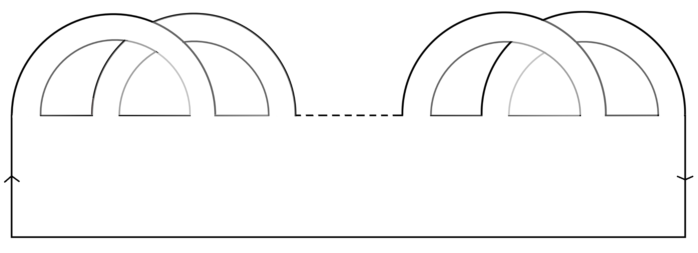
Figure 1. A Seifert surface for a knot of genus $g$.

Indeed, following ideas developed and used in [5] and [12], if you consider a knot $K$ with genus $g$ and $\Sigma$ a Seifert surface for $K$ with minimal genus, then up to isotopy, $\Sigma$ can be obtained as the thickening of a tangle $B$ with $2g$ components and $4g$ endpoints on a same horizontal line. More precisely, $B$ is a (4g-0)-tangle, and if each component $i$ of the tangle is an oriented curve $A_{i}\rightarrow B_{i}$, the points will be in the following order if you travel along the line from left to right:

$$A_{1},A_{2},B_{1},B_{2},A_{3},A_{4},B_{3},B_{4},\ldots,A_{2g-1},A_{2g},B_{2g-1},B_{2g}.$$

See Figure 2 for a drawing.

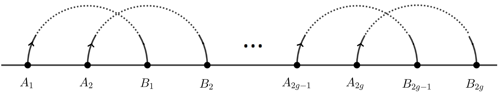
Figure 2. (4g-0)-tangle $B$.

The thickening is obtained by doubling all the components of $B$ while reversing the orientation of the right strand of each component before attaching the $8g$ endpoints to a circle using cups. Surface $\Sigma$ obtained through that process is represented in Figure 3 with $K=\partial\Sigma$. Surface $\Sigma$ has $2g$ strips attached to one disk, has one boundary component $K$, and therefore has genus $g$.

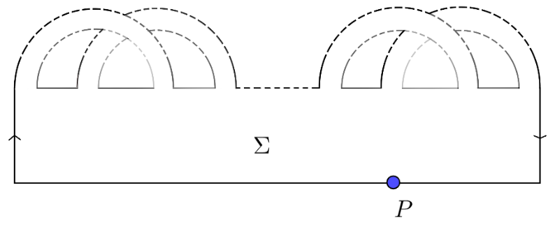
Figure 3. Embedded Seifert surface $\Sigma$ of genus $g$ for knot $K$.

When you open the disk at some point $P$ like in Figure 4, the knot gives rise to $T$ an oriented $(1-1)$-tangle for which the closure operation recovers $K$.

Figure 4. Tangle $T$.

Hopf algebra $U_{q}\mathfrak{gl}(2|1)^{\sigma}$ can be decorated with a ribbon structure (see for example [8]). Then by definition $LG(K,q,q^{\alpha})$ is obtained by the operator invariant

$$Q^{U_{q}\mathfrak{gl}(2|1)^{\sigma},V_{\alpha}}(T)$$

derived from ribbon Hopf algebra $U_{q}\mathfrak{gl}(2|1)^{\sigma}$ and irreducible representation $V_{\alpha}$, in the following way: $Q^{U_{q}\mathfrak{gl}(2|1)^{\sigma},V_{\alpha}}(T)$ is a $U_{q}\mathfrak{gl}(2|1)^{\sigma}$-linear map from irreducible $U_{q}\mathfrak{gl}(2|1)^{\sigma}$- module $V_{\alpha}$ to $V_{\alpha}$. Schur’s Lemma states that such a map acts as a scalar on $V_{\alpha}$:

$$Q^{U_{q}\mathfrak{gl}(2|1)^{\sigma},V_{\alpha}}(T)=c.id_{V_{\alpha}}$$

for some $c\in\mathbb{C}$. Constant $c$ is the value of the Links-Gould polynomial $LG(K,q,q^{\alpha})$ for a given choice of parameters $q,q^{\alpha}$.

Moreover, the topological invariance of the operator invariant allows us to compute it rather on the (1-1)-tangle that is isotopic to $T$ shown in Figure 5.

Figure 5. Tangle $T$ after isotopy.

As an operator invariant, $F(K):\mathbb{C}\rightarrow(V_{\alpha}\otimes V_{\alpha}^{\ast})^{\otimes 4g}$. As a topological object, $F(K)$ is the doubling of (4g-0)-tangle $B$ after a half-turn.

Lemma 3.2.

If $G(K)$ is the oriented $(0-4g)$-tangle obtained from $(4g-0)$-tangle $B$ after a half-turn, then:

$$Q^{U_{q}\mathfrak{gl}(2|1)^{\sigma},V_{\alpha}}(F(K))=Q^{U_{q}\mathfrak{gl}(2|1)^{\sigma},W}(G(K)).$$

Proof.

This is due to the naturality properties of the Reshetikhin-Turaev functor. ∎

Now define $\Omega^{-}:V_{\alpha}\otimes V_{\alpha}^{\ast}\rightarrow\mathbb{C}$ the negative cap derived from ribbon Hopf algebra $U_{q}\mathfrak{gl}(2|1)^{\sigma}$ using representation $V_{\alpha}$. Following De Wit’s thesis manuscript once again, it can be written in the form of a pairing between bases $(e_{1},e_{2},e_{3},e_{4})$ and $(e_{1}^{*},e_{2}^{*},e_{3}^{*},e_{4}^{*})$:

$$\Omega^{-}=\begin{pmatrix}q^{-2\alpha}&0&0&0\\ 0&-q^{-2\alpha}&0&0\\ 0&0&-q^{-2(\alpha+1)}&0\\ 0&0&0&q^{-2(\alpha+1)}\end{pmatrix}.$$

Also recall that $a:W\rightarrow V_{\alpha}\otimes V_{\alpha}^{\ast}$ and $\tilde{a}:W^{*}\rightarrow V_{\alpha}\otimes V_{\alpha}^{\ast}$ are the isomorphisms we defined and computed in the previous section.

Using this we construct two morphisms $b:W\otimes V_{\alpha}\rightarrow V_{\alpha}$ and $c:W^{*}\otimes V_{\alpha}\rightarrow V_{\alpha}$ that are expressed diagrammatically in Figure 6.

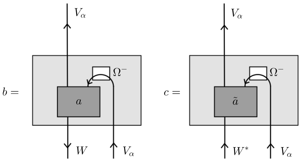
Figure 6. Maps $b$ and $c$.

This leads to the (1-1)-tangle diagram presented in Figure 7 that will be the one we will use to compute $LG(K,q,q^{\alpha})$ as an operator invariant, with $G(K):\mathbb{C}\rightarrow(W^{*}\otimes W^{*}\otimes W\otimes W)^{\otimes g}$.

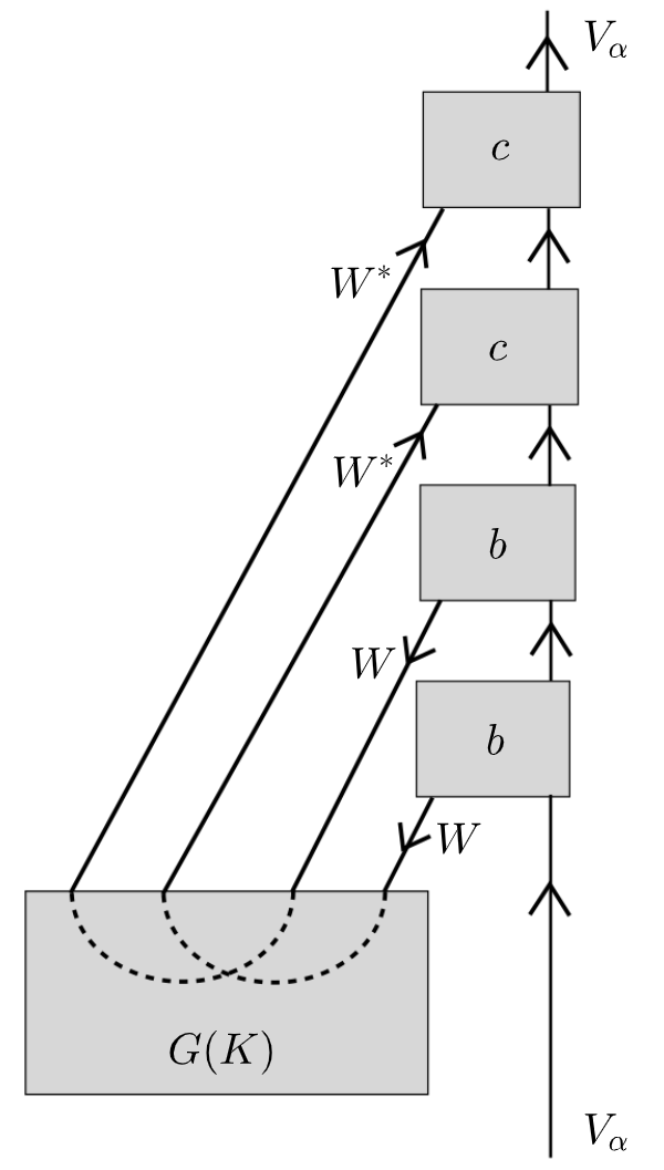
Figure 7. The diagram used to compute $LG^{2,1}$.

As a consequence of Theorem 2.12, $G(K)\in(W^{*}\otimes W^{*}\otimes W\otimes W)^{\otimes g}$ is a $\mathbb{C}(q)$-tensor and there are coefficients $\lambda_{i_{1},\ldots,i_{4g}}(q)\in\mathbb{C}(q)$ such that we can write:

$$G(K)=\displaystyle\sum_{i_{1},\ldots,i_{4g}}\lambda_{i_{1},\ldots,i_{4g}}(q)\text{ }v_{i_{1}}^{*}\otimes v_{i_{2}}^{*}\otimes v_{i_{3}}\otimes v_{i_{4}}\otimes\ldots$$

3.2. Recovering the genus bound on the (1-1)-tangle

Now we will use the (1-1)-tangle diagram described in Figure 7 to prove Theorem 1.1. The main problem we face is that the coefficients in matrices $A$ and $\tilde{A}$, that will "feed" the vector we apply to $Q^{U_{q}\mathfrak{gl}(2|1)^{\sigma},V_{\alpha}}(T)$ with degree in $q^{\alpha}$, are quite complicated. However, we are not interested in the coefficients per se. We wish to calculate an upper bound for the span of $LG(K,q,q^{\alpha})$, so in essence we want an upper bound for the highest degree monomial and a lower bound for the lowest degree monomial of the Laurent polynomial in $q^{\alpha}$ that we are considering. And naturally we would prefer these bounds not to be too loose.

To do so we will:

• first try to simplify matrices $A$ and $\tilde{A}$, and more generally morphisms $b$ and $c$ from the point of view of their action on the span of the resulting Laurent polynomial;

• then try to essentialize the different morphisms at hand as regards their contributions in terms of the highest (lowest) degree monomial in $LG(K,q,q^{\alpha})$.

Proposition 3.3.

The contribution of the negative cap $\Omega^{-}:V_{\alpha}\otimes V_{\alpha}^{\ast}\rightarrow\mathbb{C}$ to the span of $LG(K,q,q^{\alpha})$ can be ignored.

Proof.

In terms of span,

$$\Omega^{-}=\begin{pmatrix}q^{-2\alpha}&0&0&0\\ 0&-q^{-2\alpha}&0&0\\ 0&0&-q^{-2(\alpha+1)}&0\\ 0&0&0&q^{-2(\alpha+1)}\end{pmatrix}$$

can be replaced by

$$\Omega^{-}=\begin{pmatrix}1&0&0&0\\ 0&-1&0&0\\ 0&0&-q^{-2}&0\\ 0&0&0&q^{-2}\end{pmatrix}$$

in the computation of $Q^{U_{q}\mathfrak{gl}(2|1)^{\sigma},V_{\alpha}}(T)$. Indeed, this simply multiplies the polynomial by a factor $(q^{2\alpha})^{4g}$, which shifts all coefficients but does not change the span. ∎

For the same reason:

Proposition 3.4.

$\tilde{A}$ can be replaced by $q^{\alpha}\tilde{A}$ in the computation of $Q^{U_{q}\mathfrak{gl}(2|1)^{\sigma},V_{\alpha}}(T)$ without changing the span of $LG(K,q,q^{\alpha})$.

We will apply these two changes from this point on.

Definition 3.5.

Set z = $q^{\alpha}$ and $t=q^{-\alpha}$. Then for $P(q,q^{\alpha})\in\mathbb{C}(q,q^{\alpha})$, one can define $deg_{z}(P(q,q^{\alpha}))$ as the degree of the dominant coefficient in the expansion of $P(q,q^{\alpha})$ as a Laurent series in variable $z$ - if such an expansion exists. Likewise we also introduce $deg_{t}(P(q,q^{\alpha}))$.

In particular, we have:

$$deg_{z}(q^{\alpha})=deg_{z}([\alpha]_{q})=deg_{z}([\alpha+1]_{q})=1;$$

$$deg_{z}(q^{-\alpha})=deg_{z}([\alpha]_{q}^{-1})=deg_{z}([\alpha+1]_{q}^{-1})=-1;$$

$$deg_{t}(q^{-\alpha})=deg_{t}([\alpha]_{q})=deg_{t}([\alpha+1]_{q})=1;$$

$$deg_{t}(q^{\alpha})=deg_{t}([\alpha]_{q}^{-1})=deg_{t}([\alpha+1]_{q}^{-1})=-1.$$

Besides, for $P,Q$ such that the degrees exist, $deg_{z}(PQ)=deg_{z}(P)+deg_{z}(Q)$ and $deg_{t}(PQ)=deg_{t}(P)+deg_{t}(Q)$.

These remarks allow us to compute the following 4 matrices : $A_{z}=(z^{deg_{z}(Aij)})$, $A_{t}=(t^{deg_{t}(Aij)})$, $\tilde{A}_{z}=(z^{deg_{z}(\tilde{A}ij)})$ and $\tilde{A}_{t}=(t^{deg_{t}(\tilde{A}ij)})$. They will be a way to track the highest (lowest) degree monomial while computing $LG(K,q,q^{\alpha})$ through the tangle described in Figure 7. Explicitly, we have:

$$A_{z}=\blockarray{@{}ccccccccccccccccccc@{}}&\mbox{\scriptsize 1}\mbox{\scriptsize 8}\mbox{\scriptsize 9}\mbox{\scriptsize 16}\mbox{\scriptsize 2}\mbox{\scriptsize 5}\mbox{\scriptsize 15}\mbox{\scriptsize 12}\mbox{\scriptsize 3}\mbox{\scriptsize 4}\mbox{\scriptsize 14}\mbox{\scriptsize 13}\mbox{\scriptsize 6}\mbox{\scriptsize 11}\mbox{\scriptsize 10}\mbox{\scriptsize 7}\\ \block{(cccccccccccccccccc)c}1z^{2}z^{2}z^{4}000000000000\mbox{\scriptsize(1,1)}\\ 0z^{2}z^{2}z^{4}000000000000\mbox{\scriptsize(2,2)}\\ 00z^{2}z^{4}000000000000\mbox{\scriptsize(3,3)}\\ 000z^{4}000000000000\mbox{\scriptsize(4,4)}\\ 0000z^{1/2}0z^{5/2}000000000\mbox{\scriptsize(1,2)}\\ 00000z^{3/2}0z^{7/2}00000000\mbox{\scriptsize(2,1)}\\ 000000z^{5/2}000000000\mbox{\scriptsize(3,4)}\\ 0000000z^{7/2}00000000\mbox{\scriptsize(4,3)}\\ 00000000z^{1/2}0z^{5/2}00000\mbox{\scriptsize(1,3)}\\ 000000000z^{3/2}0z^{7/2}0000\mbox{\scriptsize(3,1)}\\ 0000000000z^{5/2}00000\mbox{\scriptsize(2,4)}\\ 00000000000z^{7/2}0000\mbox{\scriptsize(4,2)}\\ 000000000000z000\mbox{\scriptsize(1,4)}\\ 0000000000000z^{3}00\mbox{\scriptsize(4,1)}\\ 00000000000000z^{2}0\mbox{\scriptsize(2,3)}\\ 000000000000000z^{2}\mbox{\scriptsize(3,2)}\\$$

$\tilde{A}_{z}=$ @ccccccccccccccccccc@ & 1 8 9 16 2 5 15 12 3 4 14 13 6 11 10 7
(cccccccccccccccccc)c $1$ 0 0 0 0 0 0 0 0 0 0 0 0 0 0 0 (1,1)
$1$ $z^{-2}$ 0 0 0 0 0 0 0 0 0 0 0 0 0 0 (2,2)
$1$ $z^{-2}$ $z^{-2}$ 0 0 0 0 0 0 0 0 0 0 0 0 0 (3,3)
$1$ $z^{-2}$ $z^{-2}$ $z^{-4}$ 0 0 0 0 0 0 0 0 0 0 0 0 (4,4)
0 0 0 0 0 $z^{-3/2}$ 0 0 0 0 0 0 0 0 0 0 (1,2)
0 0 0 0 $z^{-1/2}$ 0 0 0 0 0 0 0 0 0 0 0 (2,1)
0 0 0 0 0 $z^{-3/2}$ 0 $z^{-7/2}$ 0 0 0 0 0 0 0 0 (3,4)
0 0 0 0 $z^{-1/2}$ 0 $z^{-5/2}$ 0 0 0 0 0 0 0 0 0 (4,3)
0 0 0 0 0 0 0 0 0 $z^{-3/2}$ 0 0 0 0 0 0 (1,3)
0 0 0 0 0 0 0 0 $z^{-1/2}$ 0 0 0 0 0 0 0 (3,1)
0 0 0 0 0 0 0 0 0 $z^{-3/2}$ 0 $z^{-7/2}$ 0 0 0 0 (2,4)
0 0 0 0 0 0 0 0 $z^{-1/2}$ 0 $z^{-5/2}$ 0 0 0 0 0 (4,2)
0 0 0 0 0 0 0 0 0 0 0 0 0 $z^{-3}$ 0 0 (1,4)
0 0 0 0 0 0 0 0 0 0 0 0 $z^{-1}$ 0 0 0 (4,1)
0 0 0 0 0 0 0 0 0 0 0 0 0 0 0 $z^{-2}$ (2,3)
0 0 0 0 0 0 0 0 0 0 0 0 0 0 $z^{-2}$ 0 (3,2)

$$A_{t}=\blockarray{@{}ccccccccccccccccccc@{}}&\mbox{\scriptsize 1}\mbox{\scriptsize 8}\mbox{\scriptsize 9}\mbox{\scriptsize 16}\mbox{\scriptsize 2}\mbox{\scriptsize 5}\mbox{\scriptsize 15}\mbox{\scriptsize 12}\mbox{\scriptsize 3}\mbox{\scriptsize 4}\mbox{\scriptsize 14}\mbox{\scriptsize 13}\mbox{\scriptsize 6}\mbox{\scriptsize 11}\mbox{\scriptsize 10}\mbox{\scriptsize 7}\\ \block{(cccccccccccccccccc)c}1111000000000000\mbox{\scriptsize(1,1)}\\ 0111000000000000\mbox{\scriptsize(2,2)}\\ 0011000000000000\mbox{\scriptsize(3,3)}\\ 0001000000000000\mbox{\scriptsize(4,4)}\\ 0000t^{-1/2}0t^{-1/2}000000000\mbox{\scriptsize(1,2)}\\ 00000t^{1/2}0t^{1/2}00000000\mbox{\scriptsize(2,1)}\\ 000000t^{-1/2}000000000\mbox{\scriptsize(3,4)}\\ 0000000t^{1/2}00000000\mbox{\scriptsize(4,3)}\\ 00000000t^{-1/2}0t^{-1/2}00000\mbox{\scriptsize(1,3)}\\ 000000000t^{1/2}0t^{1/2}0000\mbox{\scriptsize(3,1)}\\ 0000000000t^{-1/2}00000\mbox{\scriptsize(2,4)}\\ 00000000000t^{1/2}0000\mbox{\scriptsize(4,2)}\\ 000000000000t^{-1}000\mbox{\scriptsize(1,4)}\\ 0000000000000t00\mbox{\scriptsize(4,1)}\\ 0000000000000010\mbox{\scriptsize(2,3)}\\ 0000000000000001\mbox{\scriptsize(3,2)}\\$$

$$\tilde{A}_{t}=\blockarray{@{}ccccccccccccccccccc@{}}&\mbox{\scriptsize 1}\mbox{\scriptsize 8}\mbox{\scriptsize 9}\mbox{\scriptsize 16}\mbox{\scriptsize 2}\mbox{\scriptsize 5}\mbox{\scriptsize 15}\mbox{\scriptsize 12}\mbox{\scriptsize 3}\mbox{\scriptsize 4}\mbox{\scriptsize 14}\mbox{\scriptsize 13}\mbox{\scriptsize 6}\mbox{\scriptsize 11}\mbox{\scriptsize 10}\mbox{\scriptsize 7}\\ \block{(cccccccccccccccccc)c}1000000000000000\mbox{\scriptsize(1,1)}\\ 1100000000000000\mbox{\scriptsize(2,2)}\\ 1110000000000000\mbox{\scriptsize(3,3)}\\ 1111000000000000\mbox{\scriptsize(4,4)}\\ 00000t^{-1/2}0000000000\mbox{\scriptsize(1,2)}\\ 0000t^{1/2}00000000000\mbox{\scriptsize(2,1)}\\ 00000t^{-1/2}0t^{-1/2}00000000\mbox{\scriptsize(3,4)}\\ 0000t^{1/2}0t^{1/2}000000000\mbox{\scriptsize(4,3)}\\ 000000000t^{-1/2}000000\mbox{\scriptsize(1,3)}\\ 00000000t^{1/2}0000000\mbox{\scriptsize(3,1)}\\ 000000000t^{-1/2}0t^{-1/2}0000\mbox{\scriptsize(2,4)}\\ 00000000t^{1/2}0t^{1/2}00000\mbox{\scriptsize(4,2)}\\ 0000000000000t^{-1}00\mbox{\scriptsize(1,4)}\\ 000000000000t000\mbox{\scriptsize(4,1)}\\ 0000000000000001\mbox{\scriptsize(2,3)}\\ 0000000000000010\mbox{\scriptsize(3,2)}\\$$

Taking a careful look at these 4 matrices has several consequences.

Proposition 3.6.

$deg_{z}(LG(K,q,q^{\alpha}))\leq 8g(K).$

Proof.

Since $Q^{U_{q}\mathfrak{gl}(2|1)^{\sigma},V_{\alpha}}(T)=LG(K,q,q^{\alpha})Id_{V_{\alpha}}$, one way to compute $LG(K,q,q^{\alpha})$ is to compute $Q^{U_{q}\mathfrak{gl}(2|1)^{\sigma},V_{\alpha}}(T)(e_{1})$.

The first step is to make $e_{1}$ go through box $G(K)$. After that, the element at hand is

$$G(K)\otimes e_{1}=\sum\limits_{i_{1},\dots,i_{4g}}\lambda_{i_{1},\dots,i_{4g}}(q)\bigotimes\limits_{k=1}^{g}v_{4k-3}^{\ast}\otimes v_{4k-2}^{\ast}\otimes v_{4k-1}\otimes v_{4k}\otimes e_{1}.$$

One wants to know what happens when you compute $b(v_{i_{4g}}\otimes e_{1})$.

$$b(v_{i_{4g}}\otimes e_{1})=(Id_{V_{\alpha}}\otimes\Omega^{-})\circ(a\otimes id_{V_{\alpha}})(v_{i_{4g}}\otimes e_{1})$$

$$=Id_{V_{\alpha}}\otimes\Omega^{-}(a_{v_{i_{4g}}}\otimes e_{1}).$$

This element is equal to zero, except if $a(v_{i_{4g}})$ has a nonzero coefficient in front of $e_{1}\otimes e_{1}^{\ast}$, $e_{2}\otimes e_{1}^{\ast}$, $e_{3}\otimes e_{1}^{\ast}$ or $e_{4}\otimes e_{1}^{\ast}$. Reading matrix $A_{z}$ shows that this is the case if and only if

$$v_{i_{4g}}\in\{{v_{1},v_{8},v_{9},v_{16},v_{5},v_{12},v_{4},v_{13},v_{11}\}}.$$

In these different cases, the coefficient in front of $b(v_{i_{4g}}\otimes e_{1})$ has highest degree monomial in $z$ as follows:

In the worst case, the contribution of map $b$ to the degree in $z$ is $z^{4}$.

This would be the case regardless of the initial vector $v_{i_{4g}}\otimes e_{j}$ fed to $b$ given matrix $A_{z}$. Analog considerations prove that in the worst case scenario, the contribution of $c$ to the degree in $z$ is $z^{0}=1$.

Therefore, going through $b,b,c,c$, which is what happens when computing $Q^{U_{q}\mathfrak{gl}(2|1)^{\sigma},V_{\alpha}}(T)(e_{1})$, we obtain $z^{4}.z^{4}.1.1=z^{8}$ as the highest possible degree in $z$.

Note that this is a possible scenario, if you consider that $G(K)$ is generic, and so in that sense that bound is sharp:

Now there are $g$ boxes $(b,b,c,c)$ (where $g$ is the genus of a Seifert surface for $K$ with minimal genus), and we deduce that

$$deg_{z}(LG(K,q,q^{\alpha}))\leq 8g(K).$$

∎

Proposition 3.7.

$deg_{t}(LG(K,q,q^{\alpha}))\leq 0.$

Proof.

Like in the proof of Proposition 3.6, we compute $Q^{U_{q}\mathfrak{gl}(2|1)^{\sigma},V_{\alpha}}(T)(e_{1})$. We just have to understand what the cost of entering a box $b$ or $c$ is in terms of degree in $t$ for a vector $e_{1}$, $e_{2}$, $e_{3}$ or $e_{4}$ (and what the outcoming vector is).

This comes entirely from observing the coefficients of matrices $A_{t}$ and $\tilde{A_{t}}$, and can be summed up as follows.

• Entering in state $e_{1}$:

  

• Entering in state $e_{2}$:

  

• Entering in state $e_{3}$:

  

• Entering in state $e_{4}$:

  

Several things can be noted:

• The oriented graphs are the same for $b$ and for $c$, if everything is the same otherwise. Therefore boxes $b$ and $c$ can be identified here;

• Vectors $e_{2}$ and $e_{3}$ always play the exact same role and can be identified as well;

• These graphs are coherent weight-wise, in the sense that if in one of them, you go from $e_{i}$ to $e_{j}$ with weight $t^{x}$, then you will have the same weight $t^{x}$ for any transition from $e_{i}$ to $e_{j}$;

• These graphs are also coherent orientation-wise because if the weight for the transition from state $e_{i}$ to state $e_{j}$ is $t^{x}$, then the weight for the opposite transition from $e_{j}$ to $e_{i}$ is $t^{-x}$.

This means that if you compute the degree in $t$ for the different terms in $Q^{U_{q}\mathfrak{gl}(2|1)^{\sigma},V_{\alpha}}(T)(e_{1})$, that degree is a state function: it only depends on the term’s state, that is if it is a multiple of $e_{1}$, $e_{2}=e_{3}$, or $e_{4}$. The situation can be summed up with the following graph:

But since $Q^{U_{q}\mathfrak{gl}(2|1)^{\sigma},V_{\alpha}}(T)(e_{1})=\lambda e_{1}$, at the end of the computation all terms return to their initial state: $e_{1}$. In particular they all have the same degree in $t$ as the initial term: $0$. This proves that

$$deg_{t}(\lambda)=deg_{t}(LG(K,q,q^{\alpha}))\leq 0.$$

∎

Combining Propositions 3.6 and 3.7 proves that $span_{q^{\alpha}}(LG(K,q,q^{\alpha}))\leq 8g(K).$ Now one should remember that the degree in variables $(t_{0},t_{1})$ corresponds to the span with respect to variable $q^{2\alpha}$, which provides the inequality stated in Theorem 1.1.

4. Some interesting topological consequences

The first question that comes to mind is whether this new genus bound actually is better than the one provided by the Alexander polynomial $\Delta$. In other words, is there at least one knot $K$ such that the bound obtained using $LG$ enhances the bound produced by $\Delta$:

$$2deg(\Delta_{K}(t_{0}))<deg(LG(K,t_{0},t_{1}))\text{ ?}$$

This is indeed the case. We will in particular look at what happens for the Kinoshita-Terasaka and Conway pair of mutant knots, where both the Alexander invariant and the Levine-Tristram signature fail to detect genus.

4.1. The genus bound provided by $LG$ improves the one derived from the Alexander invariant

For prime knots of 10 or fewer crossings, the span of the Alexander invariant is always equal to the Seifert genus of the knot. There are seven prime knots with 11 crossings for which the Alexander polynomial fails to recover the 3-genus. When listed with respect to the HTW ordering for tables of prime knots of up to 16 crossings ([6]), these knots are:

$$11^{N}_{34},11^{N}_{42},11^{N}_{45},11^{N}_{67},11^{N}_{73},11^{N}_{97}\text{ and }11^{N}_{152}.$$

For four of them, the lower bound obtained using $LG$ is more precise than the one computed from $\Delta$:

$$11^{N}_{34}\text{ (the Conway knot)},11^{N}_{42}\text{ (the Kinoshita\textendash Terasaka knot)},11^{N}_{67}\text{ and }11^{N}_{97}.$$

This is explained in [9], Proposition 2.1, where the genus bound was first conjectured, and supported by empirical evidence. The list of prime knots of 12 crossings for which we get a more precise lower bound with $LG$ than with $\Delta$ can also be found in [9]. For the KT Conway pair of knots, this improvement is significant.

4.2. The Kinoshita-Terasaka and Conway pair of mutant knots

The Kinoshita–Terasaka knot ($11^{N}_{42}$) and the Conway knot ($11^{N}_{34}$) are a pair of prime knots that are related by mutation, see Figure 8.

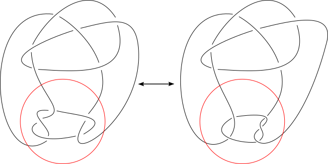
Figure 8. The Kinoshita–Terasaka knot (left), the Conway knot (right), and how they are related by mutation.

These two knots share the same Alexander invariant, as well as the same Jones polynomial. Also, their common Alexander polynomial ($=1$) and Levine-Tristram signature ($=0$) fail to say anything about the genus of either of these knots. These knots have been studied extensively, including recently, e.g. [15].

As a matter of fact, they also share the same $LG$, since $LG$ does not detect mutation. Still, the Links-Gould invariant offers a nontrivial lower bound for their genera.

Theorem 4.1.

$g(11^{N}_{34})\geq 2$ and $g(11^{N}_{42})\geq 2$.

Proof.

The value of the Links-Gould invariant for $11^{N}_{34}$ and $11^{N}_{42}$, that is the same since they are mutants, can be found in [3], section 4.9. We translate it here because it is written using the substitution $p:=q^{\alpha}$:

$$LG(11^{N}_{34}) =LG(11^{N}_{42}) = \text{ }q^{-6\alpha}(-q^{-8}-q^{-6}+2q^{-4}+q^{-2}-1)+q^{-4\alpha}(q^{-8}+6q^{-6}-3q^{-4}-9q^{-2}+2+3q^{2})$$

$$+q^{-2\alpha}(-7q^{-6}-7q^{-4}+18q^{-2}+9-11q^{2}-2q^{4})+(2q^{-6}+14q^{-4}-8q^{-2}-23$$

$$+6q^{2}+10q^{4})+q^{2\alpha}(-7q^{-4}-7q^{-2}+18+9q^{2}-11q^{4}-2q^{6})+q^{4\alpha}(q^{-4}+6q^{-2}$$

$$-3-9q^{2}+2q^{4}+3q^{6})+q^{6\alpha}(-q^{-2}-1+2q^{2}+q^{4}-q^{6}).$$

Hence, using Theorem 1.1,

$$4g(11^{N}_{34})\geq 6\text{ and }4g(11^{N}_{42})\geq 6$$

and therefore

$$g(11^{N}_{34})\geq 1,5\text{ and }g(11^{N}_{42})\geq 1,5.$$

But the genus of a knot is an integer. ∎

References

- [1] D. De Wit. The Links-Gould invariant. Ph.D. dissertation, University of Queensland, 1998. ArXiv:math/9909063, 1999.
- [2] D. De Wit, A. Ishii, J. Links. Infinitely many two-variable generalisations of the Alexander–Conway polynomial. Algebraic and Geometric Topology, Volume 5, Issue 1, 405-418, 2005.
- [3] D. De Wit, L.H. Kauffman, J. Links. On the Links-Gould invariant of links. Journal of Knot Theory and Its Ramifications, Volume 8, No. 2, 165-199, 1999.
- [4] M. Gould, K. Hibberd, J. Links, Y. Z. Zhang. Integrable electron model with correlated hopping and quantum supersymmetry. Physics Letters A, Volume 212, 156-160, 1996.
- [5] K. Habiro. Bottom tangles and universal invariants. Algebraic and Geometric Topology, Volume 6, 1113-1214, 2006.
- [6] J. Hoste, M. Thistlethwaite, J. Weeks. The first 1,701,936 knots. The Mathematical Intelligencer, 20(4), 33-48, 1998.
- [7] A. Ishii. The Links-Gould polynomial as a generalization of the Alexander-Conway polynomial. Pacific Journal of Mathematics, Volume 225, Issue 2, 273-285, 2006.
- [8] S.M. Khoroshkin, V.N. Tolstoy. Universal R-matrix for quantized (super)algebras. Communications in Mathematical Physics, Volume 141, no. 3, 599–617, 1991.
- [9] B. M. Kohli. The Links-Gould invariant as a classical generalization of the Alexander polynomial ?. Experimental Mathematics, Volume 27, Issue 3, 251-264, 2018.
- [10] B. M. Kohli. On the Links–Gould invariant and the square of the Alexander polynomial. Journal of Knot Theory and Its Ramifications, Volume 25, Issue 2, 2016.
- [11] B. M. Kohli, B. Patureau-Mirand. Other quantum relatives of the Alexander polynomial through the Links-Gould invariants. Proc. Amer. Math. Soc., Volume 145, 5419-5433, 2017.
- [12] D. López Neumann, R. Van Der Veen. Genus bounds for twisted quantum invariants. ArXiv:2211.15010, 2022.
- [13] S. Majid. Cross products by braided groups and bosonization. Journal of Algebra, 163 (1), 165-190, 1994.
- [14] K. Murasugi. On the genus of the alternting knot II. J. Math. Soc. Japan, 10 (3), 235-248, 1958.
- [15] L. Piccirillo. The Conway knot is not slice. Ann. of Math., (2) 191 (2), 581-591, 2020.
- [16] M. E. Sweedler. Hopf algebras. Mathematics Lecture Note Series, W. A. Benjamin, Inc., New York, 1969.
- [17] R. B. Zhang. Universal operator and invariants of the quantum supergroup . Journal of Mathematical Physics, Volume 33, Issue 6, 1970-1979, 1992.
- [18] R. B. Zhang. Finite dimensional irreducible representations of the quantum supergroup . Journal of Mathematical Physics, Volume 34, Issue 3, 1236-1254, 1993.