Atoms and associated spectral properties for positive operators on $L^{p}$

Abstract.

Inspired by Schwartz, Jang-Lewis and Victory, who study in particular generalizations of triangularizations of matrices to operators, we shall give for positive operators on Lebesgue spaces equivalent definitions of atoms (maximal irreducible sets). We also characterize positive power compact operators having a unique non-zero atom which appears as a natural generalization of irreducible operators and are also considered in epidemiological models. Using the different characterizations of atoms, we also provide a short proof for the representation of the ascent of a positive power compact operator as the maximal length in the graph of critical atoms.

1. Introduction and main results

1.1. Setting and main goals

We consider the Lebesgue space $L^{p}=L^{p}(\Omega,\mathcal{F},\mu)$ with $p\in(1,+\infty)$, and a state space $\Omega$ endowed with a $\sigma$-field $\mathcal{F}$ and a non-zero $\sigma$-finite measure $\mu$. Let $T$ be a positive bounded operator on $L^{p}$. For $A\in\mathcal{F}$, we denote by $T(A)$ the support of $T(\mathbb{1}_{A})$ (if $\mathbb{1}_{A}$ does not belong to $L^{p}$, then one can replace it by $f\mathbb{1}_{A}$ for any positive function $f\in L^{p}$) which is defined up to sets of $\mu$-zero measure. Then, we say a set $A\in\mathcal{F}$ is invariant if $T(A)\subset A$. A set $A$ is co-invariant if $A^{c}$ is invariant (or equivalently if $A$ is invariant for the dual operator $T^{\star}$). The collection of admissible sets corresponds to the $\sigma$-field $\mathcal{A}\subset\mathcal{F}$ generated by the invariant sets. We define the atoms as the minimal admissible sets with positive measure. An atom is non-zero if $T$ restricted to this atom is non-zero. An atom is critical if it is non-zero and the spectral radii of $T$ and of $T$ restricted to this atom are equal.

Building on works by Schwartz [25] and Jang-Lewis and Victory [17], that study in particular generalizations of triangularizations of matrices to operators, our aim in this work is threefold:

1. give several equivalent definitions of atoms,

2. describe all the nonnegative eigenfunctions of $T$ using distinguished atoms, allowing a characterization of operators $T$ having a unique non-zero atom;

3. describe all the generalized eigenfunctions of $T$ whose eigenvalue is the spectral radius of $T$, and represent the ascent of $T$ as the maximal length in the graph of critical atoms.

Except the characterization of atoms, all our results are proved under the assumption that $T$ is power compact.

We now give details on each of these aspects, discussing the relevant literature after each statement.

1.2. On atoms

For a measurable set $A$, we consider its future $F(A)$ (resp. its past $P(A)$) as the smallest invariant (resp. co-invariant) set containing $A$. When $T$ is seen as the transmission operator for an epidemic propagation, see Delmas, Dronnier and Zitt [8], the future $F(A)$ can be interpreted as the sub-population of $\Omega$ which might be infected by an epidemic starting in $A$, and $P(A)$ can be interpreted as the sub-population of $\Omega$ which may contaminate the population $A$. Motivated by the point of view of successive infections, we prove the following interpretation of the future in Corollary 3.45, for $A\in\mathcal{F}$:

$$\mathrm{e}^{T}(A)=\bigcup_{n\in\operatorname{\mathbb{N}}}T^{n}(A)=F(A).$$

We say the operator $T$ on $L^{p}$ is irreducible if its only invariant sets are a.e.  equal to $\emptyset$ or $\Omega$; in particular $F(A)=P(A)=\Omega$ for any measurable set $A$ with positive measure. We say that a set $A\in\mathcal{F}$ is irreducible if it has positive measure and the operator $T$ restricted to the set $A$ is irreducible.

Motivated by the example of Volterra operator, see Example 3.20 below for details, and by an analogy with order theory, we say that an admissible set $A$ is convex if $A=P(A)\cap F(A)$.

Our first result gives equivalent characterizations of atoms using convex sets and irreducible sets.

Theorem 1 (Equivalent definitions of atoms).

Let $T$ be a positive operator on $L^{p}$ with $p\in(1,+\infty)$. The following properties are equivalent.

1. The set $A$ is an atom.

2. The set $A$ is minimal among convex sets with positive measure.

3. The set $A$ is an admissible irreducible set.

4. The set $A$ is a maximal irreducible set.

Following [25], we also give an at most countable partition of $\Omega$ in atoms and a (possibly empty) set $\Omega_{0}$ such that $T$ restricted to each atom is irreducible; if the operator $T$ is power compact, then $T$ is quasi-nilpotent on $\Omega_{0}$.

Remark 1.1 (Related notions and results.).

Various definitions and properties of atoms already appear in the literature. Our definition of invariance and atoms are adapted from Schwartz [25], see also Victory [27, 28]. The past of a set appears in Nelson [20] (as the closure) and in Jang-Lewis and Victory [17] (as closure for bands in a Banach lattice). Irreducibility corresponds to ideal-irreducibility from Schaefer [24]. Maximal irreducible sets appear in [20] and [27] for kernel operators (where they are called components), and Omladič and Omladič [21] for more general Banach lattices (where they are called classes). Convexity of atoms is used in the proof of [25, Lemma 12]; the irreducible bands used in the Frobenius decomposition from Jang and Victory [15] are convex irreducible sets, and the semi-invariant bands, considered by Bernik, Marcoux and Radjavi [5] are in particular convex. However, to the best of our knowledge, convexity has not been studied for its own sake in this setting, and the equivalence provided by Theorem 1 is new.

Finally, the decomposition of the space in atoms and a part where $T$ is quasi-nilpotent is essentially due to Schwartz [25]. It corresponds, for nonnegative matrices, to the Frobenius normal form introduced by Victory [29], that is, a block triangularization of the matrix according to the communication classes. Notice that the triangularization of matrices has been extended to (bounded) operators in Banach spaces by Ringrose [22] using invariant spaces, see also Dowson [10, Section 2].

1.3. Nonnegative eigenfunctions

From now on we assume that the positive operator $T$ is power compact with positive spectral radius $\rho(T)>0$. For a (non-zero) eigenfunction $v$ of $T$, let $\rho(v)$ denote the corresponding eigenvalue: $Tv=\rho(v)\,v$ (and similarly for left eigenfunctions).

Let us recall briefly two key results on nonnegative eigenfunctions for positive power compact operators, see Theorem 4.2. Let $\operatorname{m}(\lambda,T)$ denote the algebraic multiplicity of $\lambda\in\operatorname{\mathbb{C}}^{*}$, that is, the dimension of $\bigcup_{k\in\operatorname{\mathbb{N}}}\mathrm{Ker}\,(T-\lambda\operatorname{Id})^{k}$. Recall that $\lambda\in\operatorname{\mathbb{C}}^{*}$ is a simple eigenvalue if $\operatorname{m}(\lambda,T)=1$. According to Krein-Rutman theorem, $\rho(T)$ is an eigenvalue of $T$, and there exists corresponding nonnegative right and left eigenfunctions. Furthermore, if $\rho(T)$ is positive and if $T$ is irreducible, the Perron-Jentzsch theorem states that the eigenvalue $\rho(T)$ is simple, and the corresponding right and left eigenfunctions are in fact positive.

Our first result characterizes monatomic operators, that is, operators having a unique non-zero atom, in terms of nonnegative eigenfunctions.

Theorem 2 (Characterization of monatomic operators).

Let $T$ be a positive power compact operator on $L^{p}$ with $p\in(1,+\infty)$ with positive spectral radius. The following properties are equivalent.

1. The operator $T$ is a monatomic.

2. There exist a unique right and a unique left nonnegative eigenfunctions of $T$ related to a non-zero eigenvalue, and $\rho(T)$ is a simple eigenvalue of $T$.

3. There exist a unique right and a unique left nonnegative eigenfunctions of $T$ related to a non-zero eigenvalue, say $u$ and $v$, and $\operatorname{supp}(u)\cap\operatorname{supp}(v)$ has positive measure.

Furthermore, when the operator $T$ is monatomic, if $u$ and $v$ denote its unique right and left nonnegative eigenfunctions, then $\rho(u)=\rho(v)=\rho(T)$ and $\operatorname{supp}(u)\cap\operatorname{supp}(v)$ is the non-zero atom.

Remark 1.2 (On monatomicity).

Monatomicity is a natural extension of irreducibility, and generalizes the notion of quasi-irreducibility defined for symmetrical operators, see Bollobás, Janson and Riordan [7, Definition 2.11]. Monatomic operators naturally appear when studying the concavity property of the function $\eta\mapsto\rho(TM_{\eta})$ where $\eta$ is a $[0,1]$-valued measurable function defined on $\Omega$ and $M_{\eta}$ the multiplication by $\eta$ operator defined on $L^{p}$, see for example Delmas, Dronnier and Zitt [9, Lemma 7.3] and its discussion for additional references in particular in epidemiology.

More generally, we may characterize nonnegative eigenfunctions in terms of the atoms appearing in their support. Let us give a few more definitions. Let $\mathfrak{A}$ denote the set of atoms (which is at most countable and might be empty); and we introduce a (partial) order $\preccurlyeq$ and the corresponding strict order $\prec$ on this set (see Proposition 3.38): for two atoms $A,B$, we write $B\prec A$ if $B\subset F(A)\setminus A$. A family of atoms is an antichain if no two atoms in the family satisfy $B\prec A$. For any atom $A$, let $\rho(A)$ be the spectral radius of the restriction of $T$ to $A$. Let us say that an atom $A$ is distinguished if, for any atom $B$, $B\prec A$ implies that $\rho(B)<\rho(A)$, and that an eigenvalue $\lambda$ is distinguished if there exists a distinguished atom $A$ with $\rho(A)=\lambda$. For $\lambda\in\operatorname{\mathbb{R}}_{+}^{*}$, we consider the (finite but possible empty) set $\mathfrak{A}(\lambda)$ of atoms with spectral radius $\lambda$ and the subset $\mathfrak{A}_{\mathrm{dist}}(\lambda)$ of distinguished atoms associated to $\lambda$:

$$\mathfrak{A}(\lambda)=\left\{A\in\mathfrak{A}\,\colon\,\rho(A)=\lambda\right\}\quad\text{and}\quad\mathfrak{A}_{\mathrm{dist}}(\lambda)=\left\{A\in\mathfrak{A}(\lambda)\,\colon\,\text{$A$ is distinguished}\right\}.$$

To any distinguished atom $A$, we may associate a unique (up to a multiplicative constant) nonnegative eigenfunction denoted $w_{A}$ such that $\operatorname{supp}(w_{A})=F(A)$ and furthermore $\rho(w_{A})=\rho(A)$ (see Lemma 4.12 iii); and then the following holds.

Theorem 3 (Characterization of nonnegative right eigenfunctions).

Let $T$ be a positive power compact operator on $L^{p}$ with $p\in(1,+\infty)$. Let $\lambda>0$. We have the following properties.

1. There exists a nonnegative eigenfunction of $T$ with eigenvalue $\lambda$ if and only if $\lambda$ is a distinguished eigenvalue.

2. The set $\mathfrak{A}_{\mathrm{dist}}(\lambda)$ is a (possibly empty) finite antichain of atoms, and the family $(w_{A})_{A\in\mathfrak{A}_{\mathrm{dist}}(\lambda)}$ is linearly independent.

3. The cone of nonnegative right eigenfunctions of $T$ with eigenvalue $\lambda$ is the conical hull of $\{w_{A}\,\colon\,A\in\mathfrak{A}_{\mathrm{dist}}(\lambda)\}$, and more precisely: if $v$ is a nonnegative eigenfunction with $\rho(v)=\lambda$, then we have:

   $$v=\sum_{A\in\mathfrak{A}_{\mathrm{dist}}(\lambda)}\mathrm{c}_{A}w_{A},$$

   where $\mathrm{c}_{A}\in\operatorname{\mathbb{R}}_{+}$, and $\mathrm{c}_{A}>0$ if and only if $A\subset\operatorname{supp}(v)$.

Remark 1.3 (Related results).

The theorem is in essence a reformulation of results by Jang-Lewis and Victory. More precisely, definitions and characterization of distinguished atoms and eigenvalues appear in [16, 17, 26, 27] ; Point i is in [17, Theorem IV.1] in the more general context of power compact operators on a Banach lattice with an order continuous norm, and Point iii appears in [27, Corollary 1] for power compact kernel operators on $L^{p}$.

The salient point of our approach is that it leverages the decomposition of the multiplicities of the eigenvalues given in [25, Theorem 7] and our characterization of atoms from Theorem 1 to provide simpler and shorter proofs.

1.4. Critical atoms and generalized eigenspace

We now give a particular attention to the atoms associated to $\rho(T)$. We define the generalized eigenspace:

$$K(T)=\bigcup\limits_{k\in\operatorname{\mathbb{N}}}\mathrm{Ker}\,\left(T-\rho(T)\operatorname{Id}\right)^{k}.$$

Following [11] and [18], we define, with the convention $\inf\emptyset=+\infty$, the ascent of $T$ at its spectral radius $\rho(T)$ by:

$$\alpha_{T}=\inf\{k\in\operatorname{\mathbb{N}}:\mathrm{Ker}\,(T-\rho(T)\operatorname{Id})^{k}=\mathrm{Ker}\,(T-\rho(T)\operatorname{Id})^{k+1}\}.$$

It is well-known, see [18], that when the operator $T$ is power compact, the ascent $\alpha_{T}$ is finite.

We say that an atom $A$ is critical when we have $\rho(A)=\rho(T)$, and we denote ${\mathfrak{A}_{\mathrm{crit}}}=\mathfrak{A}(\rho(T))$ the set of the critical atoms. For $n\geq 1$, a chain of length $n$ is a sequence $(A_{0},\dots,A_{n})$ of elements of ${\mathfrak{A}_{\mathrm{crit}}}$ such that $A_{i+1}\prec A_{i}$ for all $0\leq i<n$. The height $h(A)$ of a critical atom $A$ is one plus the maximum length of a chain starting at $A$.

Our last result is the following.

Theorem 4 (Ascent and maximal height).

Let $T$ be a positive power compact operator on $L^{p}$ with $p\in(1,+\infty)$ with positive spectral radius. Then the ascent of $T$ at its spectral radius $\rho(T)$ is equal to the maximal height of the critical atoms:

$$\alpha_{T}=\max_{A\in{\mathfrak{A}_{\mathrm{crit}}}}h(A).$$

This result is also stated in [15, 17] for positive power compact operators on Banach lattices with order continuous norm. Here also, we provide a shorter proof using properties of convex sets.

1.5. Structure of the paper

After recalling basic notions on Banach spaces in Section 2, we introduce the invariant/admissible sets and the atoms in Section 3, then we define the future and the past of a set in Section 3.2, the irreducible sets in Section 3.3, the convex sets in Section 3.5 and the order $\preccurlyeq$ in Section 3.9. We then study properties and characterizations of atoms in Sections 3.7 and 3.8, and we stress some relation between the atoms of $T$ and $T^{n}$ in Section 3.10.

To build intuition, we devote Section 3.4 to the particular case where $\Omega$ is countable, and therefore a union of atoms.

We characterize the cone of nonnegative eigenfunctions with the same eigenvalue for power compact positive operators in Section 4.2 and prove Theorem 3 (see Theorem 4.13). Section 4.3 is devoted to the proof of Theorem 2 (see Theorem 4.15) on the characterization of monatomic operators.

Section 5 is devoted to the generalized eigenfunction associated to the eigenvalue $\rho(T)$ and Theorem 4 (see Theorem 5.3 and Corollary 5.4).

2. Notations

2.1. Ordered set

Let $(E,\leq)$ be a (partially) ordered set, also called poset. Whenever it exists, the supremum of $A\subset E$, denoted by $\sup(A)$, is the least upper bound of $A$ (formally, $\sup(A)\in E$ is defined by: for all $x\in A$, $x\leq\sup(A)$ and if for some $z\in E$ one has $x\leq z$ for all $x\in A$, then $\sup(A)\leq z$). A collection $(x_{i})_{i\in\mathcal{I}}$ of elements of $E$ is an antichain if for all distinct $i,j\in\mathcal{I}$, the elements $x_{i}$ and $x_{j}$ are not comparable for the order relation. A set $D\subset E$ is a downset if for all $x\in D,y\in E$, the relation $y\leq x$ implies $y\in D$.

2.2. Banach space and Banach lattice

Let $(X,\left\lVert\,\cdot\,\right\rVert)$ be a complex Banach space not reduced to $\{0\}$. An operator $T$ on $X$ is a bounded linear (and thus continuous) map from $X$ to itself. Its operator norm is given by:

$$\left\lVert\,T\,\right\rVert_{X}=\sup\left\{\left\lVert\,T(x)\,\right\rVert\,\colon\,x\in X\text{ s.t. }\left\lVert\,x\,\right\rVert=1\right\},$$

its spectrum by $\operatorname{Sp}(T)=\{\lambda\in\operatorname{\mathbb{C}}\,\colon\,T-\lambda\operatorname{Id}\text{ has no inverse}\}$, where $\operatorname{Id}$ is the identity operator on $X$, and its spectral radius (see [23, Theorem 18.9]) by:

(1) $$\rho(T)=\sup\left\{|\lambda|\,\colon\,\lambda\in\operatorname{Sp}(T)\right\}=\lim_{n\rightarrow\infty}\left\lVert\,T^{n}\,\right\rVert_{X}^{1/n}.$$

By convention we set $T^{0}=\operatorname{Id}$.

Let $X^{\star}$ denote the (topological) dual Banach space of $X$, that is the set of all the bounded linear forms on $X$. For $x\in X$, $x^{\star}\in X^{\star}$, let $\langle x^{\star},x\rangle$ denote the duality product. For an operator $T$, the dual operator $T^{\star}$ on $X^{\star}$ is defined by $\langle T^{\star}x^{\star},x\rangle=\langle x^{\star},Tx\rangle$ for all $x\in X$, $x^{\star}\in X^{\star}$.

If $\lambda\in\operatorname{\mathbb{C}}$ and $v\in X\backslash\{0\}$ satisfy $T(v)=\lambda v$, we say that $v$ is a right eigenfunction of $T$, $\lambda$ is a right eigenvalue of $T$, and, in view of the forthcoming Corollary 4.10, shall write $\lambda=\rho(v)$. Any right eigenvalue (resp. eigenfunction) of $T^{\star}$ is called a left eigenvalue (resp. eigenfunction) of $T$. Unless there is an ambiguity, we shall simply write eigenvalue and eigenfunction for right eigenvalues and eigenfunctions.

An ordered real Banach space $(X,\left\lVert\,\cdot\,\right\rVert,\leq)$ is a real Banach space $(X,\left\lVert\,\cdot\,\right\rVert)$ with an order relation $\leq$. For any $x\in X$, we define $|x|=\sup(\{x,-x\})$ the supremum of $x$ and $-x$ whenever it exists. Following [24, Section 2], the ordered Banach space $(X,\left\lVert\,\cdot\,\right\rVert,\leq)$ is a Banach lattice if:

1. For any $x,y,z\in X,\lambda\geq 0$ such that $x\leq y$, we have $x+z\leq y+z$ and $\lambda x\leq\lambda y$.

2. For any $x,y\in X$, there exists a supremum of $x$ and $y$ in $X$.

3. For any $x,y\in X$ so that $|x|\leq|y|$, we have $\left\lVert\,x\,\right\rVert\leq\left\lVert\,y\,\right\rVert$.

Let $(X,\left\lVert\,\cdot\,\right\rVert,\leq)$ be a real Banach lattice. A vector subspace $Y$ of $X$ is an ideal if:

$$x\in Y,\,y\in X,\,|y|\leq|x|\quad\Rightarrow\quad y\in Y.$$

Let $T$ be an operator on $X$. A set $Z\subset X$ is $T$-invariant or simply invariant when there is no ambiguity, if $T(Z)\subset Z$. An operator $T$ on $X$ is positive if the positive cone $X_{+}=\{x\in X\,\colon\,x\geq 0\}$ is invariant. The operator $T$ is ideal-irreducible if the only invariant closed ideals of $X$ are $\{0\}$ and $X$, see [24, Definition 8.1].

Any Banach lattice $X$ and any operator $T$ on $X$ admits a natural complex extension. The spectrum of $T$ will be identified as the spectrum of its complex extension and denoted by $\operatorname{Sp}(T)$, furthermore by [1, Lemma 6.22], the spectral radius of the complex extension is also given by $\lim_{n\rightarrow\infty}\left\lVert\,T^{n}\,\right\rVert_{X}^{1/n}$. Moreover, by [1, Corollary 3.23], if $T$ is positive (seen as an operator on the real Banach lattice $X$), then $T$ and its complex extension have the same norm. If $S$ and $T$ are two operators on $X$, we write $T\leq S$ if the operator $S-T$ is positive. If the operators $T,S$ and $S-T$ are positive, then we have $\rho(T)\leq\rho(S)$, see [19, Theorem 4.2].

2.3. Lebesgue spaces

Let $(\Omega,\mathcal{F},\mu)$ be a measured space with $\mu$ a $\sigma$-finite measure such that $\mu(\Omega)>0$. For any $\mathcal{A}\subset\mathcal{F}$, we denote by $\sigma(\mathcal{A})$ the $\sigma$-field generated by $\mathcal{A}$. If $f,g$ are two real-valued measurable functions defined on $\Omega$, we write $f\leq g$ a.e. (resp. $f=g$ a.e.) when $\mu(\{f>g\})=0$ (resp. $\mu(\{f\neq g\})=0$), and denote $\operatorname{supp}(f)=\{f\neq 0\}$ the support of $f$. We say that a real-valued measurable function $f$ is nonnegative when $f\geq 0$ a.e., and we say that $f$ is positive, denoted $f>0$ a.e., when $\mu(\{f\leq 0\})=0$. If $A,B\subset\Omega$ are measurable sets, we write $A\subset B$ a.e. (resp $A=B$ a.e.) when $\mathbb{1}_{A}\leq\mathbb{1}_{B}$ a.e. (resp. $\mathbb{1}_{A}=\mathbb{1}_{B}$ a.e.). For the sake of clarity, we will omit to write a.e. in the proofs. We shall consider the following definition of minimal/maximal sets.

Definition 2.1 (Minimal or maximal set for a property $\mathcal{P}$).

Let $\mathcal{P}\subset\mathcal{F}$ be a class of measurable sets. We say that $A\in\mathcal{F}$ is minimal for $\mathcal{P}$ if $A\in\mathcal{P}$ and for any $B\in\mathcal{P}$ such that $B\subset A$ a.e., we have $B=\emptyset$ a.e. or $B=A$ a.e.. We say that $A\in\mathcal{F}$ is maximal for $\mathcal{P}$ if $A^{c}$ is minimal for $\{B^{c}:B\in\mathcal{P}\}$.

We will usually say “minimal + property set” for a minimal (measurable) set for the corresponding property. For example, an atom of the measure $\mu$ is any minimal measurable set with positive measure, that is, any minimal set of $\mathcal{P}=\{A\in\mathcal{F}\,\colon\,\mu(A)>0\}$.

Lemma 2.2 (Existence of a minimal set).

Let $\mathcal{P}\subset\mathcal{F}$ be a class of measurable sets stable by countable intersection. Then there exists a measurable set minimal for $\mathcal{P}$.

Proof.

We recall, see [13, Appendix A.5] (where the result is stated for $\mu$ a probability measure, but can be easily extended to a $\sigma$-finite measure), that if $\{f_{i}\,\colon\,i\in I\}$ is a (possibly uncountable) family of $[-\infty,+\infty]$-valued measurable defined on $\Omega$, then there exists a $[-\infty,+\infty]$-valued measurable function $f$, called the essential infimum of $\{f_{i}:i\in I\}$ such that:

1. For all $i\in I$, $f_{i}\geq f$ a.e..

2. If $g$ is another $[-\infty,+\infty]$-valued measurable function satisfying (i), then a.e. $f\geq g$.

Furthermore, there exists an at most countable set $I^{\prime}\subset I$ such that a.e. $f=\inf_{i\in I^{\prime}}f_{i}$.

We consider $f$ the essential infimum of $\{\mathbb{1}_{B}\,\colon\,B\in\mathcal{P}\}$. Thus, there exists an at most countable set $\mathcal{P}^{\prime}\subset\mathcal{P}$ such that a.e. $f=\inf_{B\in\mathcal{P}^{\prime}}\mathbb{1}_{B}$, that is a.e.  $f=\mathbb{1}_{B^{\prime}}$ with $B^{\prime}=\bigcap_{B\in\mathcal{P}^{\prime}}B$. Since $\mathcal{P}$ is stable by countable intersection, we get that $B^{\prime}$ belongs to $\mathcal{P}$. Property (i) above on the essential infimum implies also that $B^{\prime}\subset B$ a.e.  for all $B\in\mathcal{P}$. Thus the set $B^{\prime}$ is minimal for $\mathcal{P}$. This provides the existence of a minimal set for $\mathcal{P}$. ∎

For a measurable function $f$, we write $\mu(f)=\int f\,\mathrm{d}\mu=\int_{\Omega}f(x)\,\mu(\mathrm{d}x)$ the integral of $f$ with respect to $\mu$ when it is well defined. For $p\in(1,+\infty)$, the Lebesgue space $L^{p}(\Omega,\mathcal{F},\mu)$ is the set of all real-valued measurable functions $f$ defined on $\Omega$ whose $L^{p}$-norm, $\left\lVert\,f\,\right\rVert_{p}=\mu(|f|^{p})^{1/p}$, is finite and where functions which are a.e. equal are identified. When there is no ambiguity we shall simply write $L^{p}(\Omega)$ or $L^{p}$. The set $(L^{p},\left\lVert\,\cdot\,\right\rVert_{p})$ is a Banach space with dual $(L^{q},\left\lVert\,\cdot\,\right\rVert_{q})$, where $1/p+1/q=1$. The duality product is thus $\langle g,f\rangle=\int fg\,\mathrm{d}\mu$ for $f\in L^{p}$ and $g\in L^{q}$. The Banach space $L^{p}$ endowed with the usual order $f\leq g$, that is $\mu(\{f>g\})=0$, is a Banach lattice. The positive cone $L^{p}_{+}$ is the subset of $L^{p}$ of nonnegative functions. According to [30, Section 2] and [24, Theorem 5.14, p.94], its closed ideal are the sets:

(2) $$L^{p}_{A}=\left\{f\in L^{p}\,\colon\,f\mathbb{1}_{A^{c}}=0\right\},$$

where $A\subset\Omega$ is measurable.

Let $T$ be an operator on $L^{p}$. Thanks to [12, Corollary 1.3], $T$ and its complex extension on the natural complex extension of $L^{p}$ have the same $L^{p}$-norm. Let $A\subset\Omega$ be measurable. We define the restriction operator of $T$ on $A$, denoted $T_{A}$, by:

(3) $$T_{A}=M_{A}\,T\,M_{A},\quad\text{where the operator $M_{A}$ is the multiplication by $\mathbb{1}_{A}$},$$

and, if $\mu(A)>0$, we denote by $T|_{A}$ the corresponding operator on $L^{p}(A)$, where the set $A$ is endowed with the trace of $\mathcal{F}$ on $A$ and the measure $\mu|_{A}(\cdot)=\mu(A\cap\cdot)$. When there is no ambiguity on the operator $T$, we simply write $\rho(A)$ for the spectral radius of $T_{A}$ (and of $T|_{A}$). In particular, we have $\rho(\Omega)=\rho(T)$ and $\rho(A)=0$ if $\mu(A)=0$. If the operator $T$ is positive, we also have that:

$$A\subset B\quad\Longrightarrow\quad\rho(A)\leq\rho(B).$$

A kernel $k$ is a measurable nonnegative function defined on $(\Omega^{2},\mathcal{F}^{\otimes 2})$. When possible, we define for a real-valued measurable function $f$ defined on $\Omega$ the function $T_{k}(f)$ by:

(4) $$T_{k}(f)(x)=\int_{\Omega}k(x,y)f(y)\,\mu(\mathrm{d}y)\quad\text{for}\quad x\in\Omega.$$

When it is well defined as an operator on $L^{p}$, we call $T_{k}$ the kernel operator associated to $k$.

3. Atomic decomposition of a positive operator

We consider the Lebesgue space $L^{p}=L^{p}(\Omega,\mathcal{F},\mu)$ with $\mu$ a non-zero $\sigma$-finite measure and $p\in(1,+\infty)$. In this section, we introduce the notion of invariant set, in order to provide different characterizations of the atoms of a positive bounded operator on $L^{p}$.

3.1. Invariance and atoms

The ideal-irreducibility of an operator can be described in terms of sets rather than functions. We follow the presentation of Schwartz [25] (notice $\mu$ is assumed to be finite therein).

Let $T$ be a positive operator on $L^{p}$. Let $f\in L^{p}$ and $g\in L^{q}$ be two positive functions (with $1/p+1/q=1$). We define the nonnegative function $k^{[g,f]}_{T}$ on $\mathcal{F}^{2}$ as, for $A,B\in\mathcal{F}$:

$$k^{[g,f]}_{T}(B,A)=\langle g\mathbb{1}_{B},\,T(f\mathbb{1}_{A})\rangle=\int_{B}g(x)\,T(f\mathbb{1}_{A})(x)\,\mu(\mathrm{d}x).$$

Notice that:

(5) $$k^{[f,g]}_{T^{\star}}=k^{[g,f]}_{T}.$$

We shall consider the zeros of $k^{[g,f]}_{T}$, that is the set:

(6) $$\mathcal{Z}_{T}=\{(B,A)\in\mathcal{F}^{2}:k^{[g,f]}_{T}(B,A)=0\}.$$

Let us stress that the set $\mathcal{Z}_{T}$ does not depend on the choice of the positive functions $f\in L^{p}$ and $g\in L^{q}$; this is indeed a direct consequence of the following equivalences:

(7) $$k^{[g,f]}_{T}(B,A)=0\,\Longleftrightarrow\,\mathbb{1}_{B}T(f\mathbb{1}_{A})=0\text{ a.e.}\,\Longleftrightarrow\,T^{\star}(g\mathbb{1}_{B})\mathbb{1}_{A}=0\text{ a.e.}.$$

For this reason, as long as we consider the zeros of $k^{[g,f]}_{T}$, when there is no ambiguity, we shall simply write:

(8) $$k_{T}=k^{[g,f]}_{T}.$$

Notice that for any $A\in\mathcal{F}$, the maps $k_{T}(\cdot,A)$ and $k_{T}(A,\cdot)$ on $\mathcal{F}$ are $\sigma$-additive and nonnegative. We can now introduce the definition of invariant set.

Definition 3.1 (Invariant and co-invariant sets).

Let $T$ be a positive operator on $L^{p}$ with $p\in(1,+\infty)$. A set $A$ is $T$-invariant or simply invariant if it is measurable and $k(A^{c},A)=0$; it is $T$-co-invariant or simply co-invariant if $A^{c}$ is $T$-invariant. We denote by $\mathcal{I}$ the class of the invariant sets.

If $A$ is an invariant set and $B=A\text{ a.e.}$, then $B$ also is invariant. Note also that $A$ is $T$-co-invariant if and only if $A$ is $T^{\star}$-invariant thanks to (5), and that the following equivalences hold:

(9) $$A\text{ is invariant}\quad\Longleftrightarrow\quad\exists h\in L^{p}_{+},\,\,\operatorname{supp}(h)=A,\,\text{ and }\,\,T(h)=0\,\text{ on }\,A^{c}.$$

The next lemma is a direct consequence of the $\sigma$-additivity of $k_{T}$.

Lemma 3.2 (Countable union and intersection of invariant sets).

Any at most countable union or intersection of invariant (resp. co-invariant) sets is invariant (resp. co-invariant).

We have the following characterization of invariance using closed ideals.

Lemma 3.3 (Invariant sets and invariant closed ideals).

Let $T$ be a positive operator on $L^{p}$ with $p\in(1,+\infty)$, and $A$ a measurable set. The set $A$ is $T$-invariant if and only if the closed ideal $L^{p}_{A}$ is $T$-invariant.

Proof.

We first assume that $A$ is invariant. Let $h\in L^{p}_{A}$, that is $h\in L^{p}$ and $h\mathbb{1}_{A^{c}}=0$. Let $f^{\prime}\in L^{p}$ and $g\in L^{q}$ be positive and set $f=f^{\prime}+|h|$. Since $A$ is invariant, we have $k^{[g,f]}_{T}(A^{c},A)=0$. This gives:

$$0=\langle g\mathbb{1}_{A^{c}},T(f\mathbb{1}_{A})\rangle\geq\langle g\mathbb{1}_{A^{c}},T(|h|)\rangle\geq\langle g\mathbb{1}_{A^{c}},|T(h)|\rangle\geq 0,$$

where we used the positivity of $T$ for the inequalities. We get that $T(h)\mathbb{1}_{A^{c}}=0$, that is, $T(h)\in L^{p}_{A}$. Thus the ideal $L^{p}_{A}$ is invariant.

We now assume that the ideal $L^{p}_{A}$ is invariant. For $f\in L^{p}$ and $g\in L^{q}$ positive, we have that $g\mathbb{1}_{A^{c}}T(f\mathbb{1}_{A})=0$. Therefore $k^{[g,f]}_{T}(A^{c},A)=0$, thus the set $A$ is invariant. This ends the proof. ∎

Example 3.4 (The Volterra operator).

We consider the measured space $(\Omega=[0,1],\mathcal{F}=\mathcal{B}([0,1]),\operatorname{Leb})$, with $\mathcal{F}$ the Borel subsets of $[0,1]$ and $\operatorname{Leb}$ the Lebesgue measure on $[0,1]$, and the kernel $k$ on $[0,1]$ defined by:

$$k(x,y)=\mathbb{1}_{\{x\geq y\}}\quad\text{for $x,y\in[0,1]$}.$$

The corresponding kernel operator $T_{k}$ given by (4) is the so-called Volterra operator (see [4] for some spectral and compactness properties of Volterra operators). One can see that a measurable set $A\subset[0,1]$ is $T_{k}$-invariant (resp. $T_{k}$-co-invariant) if and only if $A=[a,1]$ a.e. (resp. $A=[0,a]$ a.e.) with $a\in[0,1]$.

We give an immediate application of Lemma 3.3.

Lemma 3.5 ($T$ and $T^{n}$ invariant sets).

Let $T$ be a positive operator on $L^{p}$ with $p\in(1,+\infty)$ and $n\in\operatorname{\mathbb{N}}^{*}$. Any $T$-invariant set is $T^{n}$-invariant.

We give another example of invariant sets, that will be useful later on.

Lemma 3.6 (The support of a nonnegative eigenfunction is invariant).

Let $T$ be a positive operator on $L^{p}$ with $p\in(1,+\infty)$ and $v$ be a nonnegative right eigenfunction of $T$. Then the support of $v$ is an invariant set: $\operatorname{supp}(v)\in\mathcal{I}$.

Proof.

Let $f\in L^{p}$ be positive such that $f\mathbb{1}_{\{v>0\}}=v$, and $g\in L^{q}$ positive. We have:

$$k^{[g,f]}_{T}(\operatorname{supp}(v)^{c},\operatorname{supp}(v))=\langle g\mathbb{1}_{\{v=0\}},T(f\mathbb{1}_{\{v>0\}})\rangle=\langle g\mathbb{1}_{\{v=0\}},T(v)\rangle=\rho(v)\,\langle g\mathbb{1}_{\{v=0\}},v\rangle=0,$$

where we used that $f\mathbb{1}_{\{v>0\}}=v$ for the second equality and that $v$ is an eigenfunction of $T$ with eigenvalue $\rho(v)$ for the third one. This proves that the set $\operatorname{supp}(v)$ is $T$-invariant as the zeros of the map $k^{[g,f]}_{T}$ does not depend on the choice of the positive functions $f$ and $g$. ∎

In some cases, invariance is the same for an operator and its resolvent.

Lemma 3.7 (Resolvent of a positive operator).

Let $T$ be a positive operator on $L^{p}$ with $p\in(1,+\infty)$. If $\lambda\in\mathbb{R}$ satisfies $\lambda>\rho(T)$, then the operator $\lambda\operatorname{Id}-T$ is invertible, and its inverse is a positive operator on $L^{p}$. Moreover, the $(\lambda\operatorname{Id}-T)^{-1}$-invariant sets are exactly the $T$-invariant sets.

Proof.

Since we have $\lambda>\rho(T)$, the operator $(\lambda\operatorname{Id}-T)$ is invertible, and its inverse is given by its Neumann series:

$$(\lambda\operatorname{Id}-T)^{-1}=\sum\limits_{n=0}^{+\infty}\lambda^{-n-1}T^{n}.$$

This proves both that the operator $(\lambda\operatorname{Id}-T)^{-1}$ is positive and, thanks to Lemma 3.5, that its invariant sets are exactly the $T$-invariant sets. ∎

Following [25], we consider the atoms associated to $T$.

Definition 3.8 (Admissible set and atoms).

Let $T$ be a positive operator on $L^{p}$ with $p\in(1,+\infty)$. A set which belongs to the $\sigma$-field $\mathcal{A}=\sigma(\mathcal{I})$ generated by the family $\mathcal{I}$ of invariant sets is called admissible. A minimal admissible set with positive measure is called an atom of the operator $T$ or $T$-atom.

Notice that a set of positive measure $A$ is a $T$-atom if and only if it is an atom for the measured space $(\Omega,\mathcal{A},\mu)$. We denote by $\mathfrak{A}$ the set of atoms:

$$\mathfrak{A}=\{A\in\mathcal{A}\,\colon\text{$A$ is a $T$-atom}\}.$$

Since atoms have positive measure and the measure $\mu$ is $\sigma$-finite, we deduce that the set $\mathfrak{A}$ is at most countable. When there is no ambiguity on the operator $T$, we shall simply write atom for $T$-atom. We present Example 3.9 below where there is no atom, and Example 3.10 where not all measurable sets are admissible.

Example 3.9 (The Volterra operator).

In Example 3.4 on the Volterra operator $T_{k}$, the admissible $\sigma$-field is the Borel $\sigma$-field on $[0,1]$: $\mathcal{A}=\mathcal{F}$. Notice that the operator $T_{k}$ has no atom: $\mathfrak{A}=\emptyset$.

Example 3.10 ($\mathcal{A}\neq\mathcal{F}$).

We consider the measured space $(\Omega=[0,1],\mathcal{F}=\mathcal{B}([0,1]),\operatorname{Leb})$, with $\mathcal{F}$ the Borel subsets of $[0,1]$ and $\operatorname{Leb}$ the Lebesgue’s measure on $[0,1]$, and the kernel $k$ on $[0,1]$ defined by:

(10) $$k(x,y)=\mathbb{1}_{\{x\leq 1/2\leq y\leq x+1/2\}}+\mathbb{1}_{\{x\geq 1/2\}}\mathbb{1}_{\{y\leq x-1/2\}}\quad\text{(see Fig.\leavevmode\nobreak\ \ref{fig:kernel_1})}.$$

Let $A\subset[0,1]$ be a measurable set. Then $A$ is $T_{k}$-invariant if and only if for a.e. $x\in A^{c}\cap[0,1/2]$, we have $\operatorname{Leb}\left(\left[1/2,x+1/2\right]\cap A\right)=0$ and for a.e. $x\in A^{c}\cap[1/2,1]$, we have $\operatorname{Leb}\left(\left[0,x-1/2\right]\cap A\right)=0$. Thus, $A$ is $T_{k}$-invariant if and only if for a.e. $x\in A^{c}\cap[0,1/2]$, we have $\left[1/2,x+1/2\right]\subset A^{c}\text{ a.e.}$ and for a.e. $x\in A^{c}\cap[1/2,1]$, we have $\left[0,x-1/2\right]\subset A^{c}\text{ a.e.}$. Thus $A$ is $T_{k}$-invariant if and only if $A=[a,1/2]\cup[a+1/2,1]$ a.e. with $a\in[0,1/2]$. Therefore the $\sigma$-field $\mathcal{A}$ of $T_{k}$-admissible sets consists in all the measurable sets which are a.e. equal to $A\cup(A+1/2)$ where $A\subset[0,1/2]$ is a Borel set. In particular, we have $\mathcal{A}\neq\mathcal{F}$. Notice the operator $T_{k}$ has no atom: $\mathfrak{A}=\emptyset$.

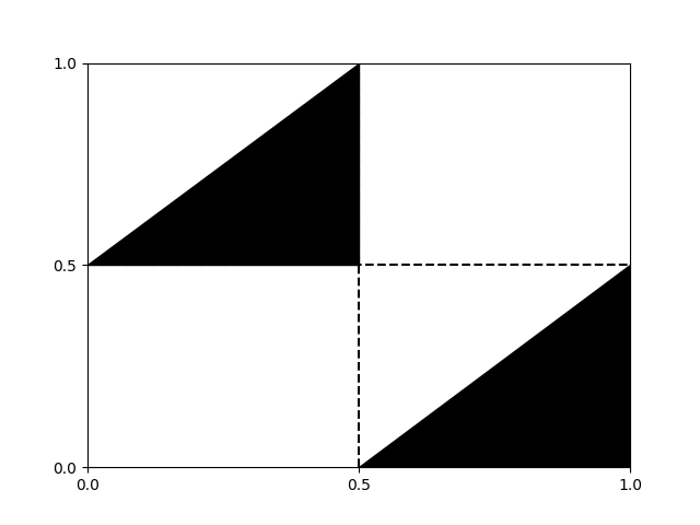
(a) Kernel $k$ defined in (10).

(b) Kernel $k^{\otimes 2}$ defined in (15).

Figure 1. Example of some $[0,1]$-valued kernels on $[0,1]$.

3.2. Future and Past

We now consider the future and past of a set, and refer to Remark 3.17 below for an epidemiological interpretation. Recall the Definition 2.1 on minimal and maximal set.

Definition 3.11 (Future and past).

Let $T$ be a positive operator on $L^{p}$ with $p\in(1,+\infty)$. Let $A$ be a measurable set. We define its future, $F(A)$, as the minimal invariant set containing $A$ (that is, the minimal set of $\mathcal{P}=\{B\in\mathcal{I}\,\colon\,A\subset B\text{ a.e.}\}$) and its past, $P(A)$, as the minimal co-invariant set containing $A$.

We shall use later on the following notation for the future and past of a set $A$ without $A$:

(11) $$F^{*}(A)=F(A)\cap A^{c}\quad\text{and}\quad P^{*}(A)=P(A)\cap A^{c}.$$

The next lemma ensures the existence of the future and the past.

Lemma 3.12 (Existence of future and past).

Let $A\in\mathcal{F}$, then its future and its past exist and are unique, up to an a.e. equality.

Proof.

We only consider the future, as the proof concerning the past is similar. The set $\mathcal{P}=\{B\in\mathcal{I}\,\colon\,A\subset B\text{ a.e.}\}$ is stable by countable intersection thanks to Lemma 3.2. Lemma 2.2 ensures the existence of a minimal set for $\mathcal{P}$. The uniqueness is also clear. This provide the existence of the future of $A$. ∎

Let us mention that the “$k$-closure” of a set for a kernel operator $T_{k}$ introduced by Nelson [20, p. 714] correspond to its past (with respect to the invariant sets associated to $T_{k}$). Let us gather without proof a number of elementary facts.

Lemma 3.13 (Basic properties of the future of a measurable set).

For any measurable sets $A$ and $B$, and for any at most countable family of measurable sets $(A_{i})_{i\in I}$, the following properties hold:

1. $F(\emptyset)=\emptyset\text{ a.e.}$ and $F(\Omega)=\Omega\text{ a.e.}$.

2. A set $A$ is invariant if and only if $F(A)=A\text{ a.e.}$.

3. If $A\subset B\text{ a.e.}$, then $F(A)\subset F(B)\text{ a.e.}$.

4. $F\left(\bigcup_{i\in I}A_{i}\right)=\bigcup_{i\in I}F(A_{i})\text{ a.e.}$.

5. $F\left(\bigcap_{i\in I}A_{i}\right)\subset\bigcap_{i\in I}F(A_{i})\text{ a.e.}$; the reverse inclusion does not hold in general.

6. $F(F(A))=F(A)\text{ a.e.}$.

The properties (i-vi) also hold with $F$ replaced by $P$.

Futures and pasts are related by the following elementary result; by contrast, note that the inclusion $A\subset F(B)$ does not imply that $B\subset P(A)$ in general, see Example 3.18.

Lemma 3.14 (Intersection of a future and a past).

Let $A,B$ be two measurable sets. We have:

$$A\cap P(B)=\emptyset\text{ a.e.}\iff F(A)\cap P(B)=\emptyset\text{ a.e.}\iff F(A)\cap B=\emptyset\text{ a.e.}.$$

Proof.

If $A\cap P(B)=\emptyset$, then $A$ in included in $P(B)^{c}$. Since the set $P(B)^{c}$ is invariant, we have $F(A)\subset P(B)^{c}$ by minimality, which means that $F(A)\cap P(B)=\emptyset$. The converse is clear since $A\subset F(A)$. The second equivalence is proved similarly. ∎

3.3. Irreducibility

Similarly to Schaefer [24, Definition 8.1], we can define the irreducibility of an operator in terms of invariance.

Definition 3.15 (Irreducible operators and invariant sets).

Let $T$ be a positive operator on $L^{p}$ with $p\in(1,+\infty)$.

1. The operator $T$ is irreducible if its only invariant sets are a.e. equal to $\emptyset$ or $\Omega$.

2. The measurable set $A$ is $T$-irreducible or simply irreducible if it is measurable with positive measure and if the restricted operator $T|_{A}$ on $L^{p}(A)$ is irreducible.

We refer to Lemma 3.30 and Theorem 3.34 for relations between irreducible sets and atoms. See also Example 3.42 for a comment on the irreducible sets of $T$ and of $T^{2}$. We now state explicitly the relation between invariance and irreducibility from Section 2.2 and from Definitions 3.1 and 3.15. Recall the definition of the closed ideal in (2).

Lemma 3.16.

Let $T$ be a positive operator on $L^{p}$ with $p\in(1,+\infty)$. Then the operator $T$ is irreducible if and only if it is ideal-irreducible.

Proof.

It is a direct consequence of Lemma 3.3 and the fact that the closed ideals of $L^{p}$ are exactly given by $L^{p}_{A}$ for $A$ measurable, see [30, Section 2] and [24, Theorem 5.14, p. 94]. ∎

3.4. The countable case and an underlying preorder

We assume in this section only that $\Omega$ is at most countable, and without loss of generality that $\mu(\{x\})>0$ for all $x\in\Omega$. Let $T$ be a positive operator on $L^{p}$. The the map $k_{T}$ is entirely defined by the values of $k_{T}(\{x\},\{y\})$, denoted $k_{T}(x,y)$, for $x,y\in\Omega$. The notions of admissibility, atoms, invariance and irreducibility may in that case be completely understood by studying a particular binary relation on $\Omega$ given in terms of $k_{T}$. To see this, we write $x\preccurlyeq y$ if $x=y$ or if there exists $n\in\operatorname{\mathbb{N}}^{*}$ and $(x=x_{0},x_{1},...,x_{n-1},x_{n}=y)\in\Omega^{n+1}$ such that $\prod_{i=1}^{n}k_{T}(x_{i-1},x_{i})>0$. The relation $\preccurlyeq$ defines a preorder on $\Omega$ (that is, a reflexive transitive binary relation). The relation $x\sim y\iff(x\preccurlyeq y\text{ and }y\preccurlyeq x)$ is then an equivalence relation. The equivalence classes of $\sim$ correspond to atoms of the operator $T$, and the preorder $\preccurlyeq$ naturally induces a (partial) order on them: for two atoms $A$, $B$, we have $A\preccurlyeq B$ if $x\preccurlyeq y$ for all $x\in A$ and $y\in B$. The admissible sets are the sets $A$ that may be written as unions of atoms (the $\sigma$-field $\mathcal{A}$ is generated by the set of atoms). Furthermore, a set $A$ is invariant if and only if the two following conditions hold:

• $A$ is the union of atoms $(A_{i})_{i\in I}$ (in particular, $A$ is admissible),

• The family $(A_{i})_{i\in I}$ is a downset for the order induced by $\preccurlyeq$ on atoms.

For a set $A$, its future corresponds to the downward closure of $A$, that is, the smallest downset containing $A$, and its future and past are given by:

$$F(A)=\bigcup_{x\in A}\{y\in\Omega\,\colon\,y\preccurlyeq x\}\quad\text{and}\quad P(A)=\bigcup_{x\in A}\{y\in\Omega\,\colon\,x\preccurlyeq y\}.$$

Notice the definition of atoms, invariant sets, future and past of a set depends only on the support $\{k_{T}>0\}\subset\Omega^{2}$ of the kernel $k_{T}$.

Remark 3.17 (Epidemiological interpretation).

In the epidemiological interpretation where each element of $\Omega$ is seen as an individual or an homogeneous sub-population and $T$ can be assimilated to the next generation operator, we have:

• $k_{T}(x,y)>0$ means that individual $y$ can directly infect individual $x$;

• $x\preccurlyeq y$ when there may be a chain of infections from individual $y$ to individual $x$;

• the set $A$ is invariant if an epidemic started in $A$ stays within $A$;

• the future $F(A)$ of $A$ is the set of all individuals that might get infected by an epidemic starting at every individual of $A$;

• the past $P(A)$ of $A$ is the set of all individuals that might infect an individual of $A$.

In Section 3.5 we shall consider convex sets, that is, sets $A$ such that $A=F(A)\cap P(A)$. They have a simple representation when $\Omega$ is at most countable. Following the terminology of [6, Section I.4, p. 7], for $x,y\in\Omega$, we define the interval $[x,y]=\{z\in\Omega\,\colon\,x\preccurlyeq z\preccurlyeq y\}$, and say that a set $A\subset\Omega$ is (order-)convex if:

$$x,y\in A\quad\implies\quad[x,y]\subset A.$$

It is easily checked that an order-convex set corresponds to being the union of atoms $(A_{i})_{i\in I}$ where the family $(A_{i})_{i\in I}$ is order convex, that is, if $A$ is an atom such that $A_{i}\preccurlyeq A\preccurlyeq A_{i^{\prime}}$ for some $i,i^{\prime}\in I$, then $A$ belongs to the family $(A_{i})_{i\in I}$.

$\begin{pmatrix}0&\star&0&0&0&0\\ \star&0&\star&0&0&0\\ 0&\star&0&0&0&0\\ 0&\star&0&0&0&0\\ 0&\star&0&0&0&0\\ 0&0&0&\star&\star&0\\ \end{pmatrix}$

(a) Matrix on $\{1,\ldots,6\}$ with $\star>0$.

(b) Associated communication graph.

Figure 2. Matrix and associated communication graph from Example 3.18.

Example 3.18 (A finite elementary case).

We consider the finite case: $\Omega=\{1,\ldots,n\}$ with $n\in\operatorname{\mathbb{N}}^{*}$, $\mu$ is the counting measure, $L^{p}(\Omega)$ is identified with $\operatorname{\mathbb{R}}^{n}$ and operators on $L^{p}$ with $n\times n$ real matrices. A matrix $M=(M_{i,j})_{1\leq i,j\leq n}$ with nonnegative entries is alternatively represented by the oriented weighted graph $G=(V,E)$ with $V=\{1,\dots,n\}$ and with a weight $M_{i,j}$ to the edge $(j,i)\in E$.

To illustrate, consider the case $n=6$ with the matrix given in Fig. 2(a) where the $\star$ correspond to positive terms. The corresponding communication graph (an oriented edge is represented for each positive entry of the matrix) is given in Fig. 2(b). The atoms are: $\{1,2,3\}$, $\{4\}$, $\{5\}$ and $\{6\}$. The invariant sets are: $\Omega$, $\{4,5,6\}$, $\{4,6\}$, $\{5,6\}$, $\{6\}$ and $\emptyset$. For example the sets $\{1,2,3\}$, $\{1,2\}$ and $\{1\}$ are irreducible, and among those three only the first one is admissible. For example the sets $\{1,2,3,4\}$, $\{5\}$ and $\{5,6\}$ are convex. Even though the set $\{5\}^{c}$ is admissible, it is not convex.

Let us notice that the inclusion in Lemma 3.13 v is not an equality in general; indeed we have: $F(\{4\}\cap\{5\})=F(\emptyset)=\emptyset$ whereas $F(\{4\})\cap F(\{5\})=\{6\}$. Notice also that $\{5\}$ belongs to the future of $\{1,2,3,4\}$, but the latter does not belong to the past of $\{5\}$.

The countable state space $\Omega$ and the above representation of convex sets will guide many definitions and proofs below. The general case is at the same time more technical (invariant sets are defined up to an a.e. equality), and more subtle: for example, the union of all atoms may be a strict subset of the whole space; it may even be empty, as in Example 3.9 where there exists no atom of the Volterra operator. For this reason we will work only on invariant and co-invariant sets, viewing them intuitively as down- and up-sets of an underlying order that we will not write down formally.

3.5. Order-convex subsets

By construction of the future and the past, a measurable set $A$ is always included in $F(A)\cap P(A)$. The set $A$ is convex when there is equality.

Definition 3.19 (Order-convex subset).

Let $T$ be a positive operator on $L^{p}$ with $p\in(1,+\infty)$. A set $A$ is order-convex for $T$, or $T$-convex, if it is measurable and $A=F(A)\cap P(A)\text{ a.e.}$.

When there is no ambiguity on the operator $T$, we shall simply write convex for $T$-convex.

Example 3.20 (Convex sets of the Volterra operator).

We continue Example 3.4 on the Volterra operator. Using the description therein of invariant and co-invariant sets, we get that a set $A$ is convex if and only if $A=[a,b]$ a.e.  with $0\leq a\leq b\leq 1$.

Remark 3.21 (Atoms, irreducibility and convexity coincide for $T$ and $T^{\star}$).

Notice that the admissible $\sigma$-field is the same for the operator $T$ and its dual $T^{\star}$. Thanks to (5), the operator $T$ is irreducible if and only if $T^{\star}$ is irreducible. Thus a set $A$ is a $T$-atom (resp. $T$-irreducible, $T$-convex) if and only if it is a $T^{\star}$-atom (resp. $T^{\star}$-irreducible, $T^{\star}$-convex).

Remark 3.22 (Convex sets on a countable measurable set).

We go back to the framework of subsection 3.4, where $\Omega$ is an at most countable set. Then $A$ is a convex set in the sense of Definition 3.19 if and only if $A$ is order-convex in the sense of the definition of subsection 3.4. Therefore the two definitions are coherent.

Recall (11), where we set $F^{*}(A)=F(A)\cap A^{c}$ and $P^{*}(A)=P(A)\cap A^{c}$.

Lemma 3.23 (Characterization of convexity).

Let $A$ be a measurable set. The following properties are equivalent:

1. $A$ is convex.

2. $F^{*}(A)\cap P^{*}(A)=\emptyset\text{ a.e.}$.

3. $F^{*}(A)$ is invariant.

4. $P^{*}(A)$ is co-invariant.

5. There exist an invariant set $B$ and a co-invariant set $C$ such that $A=B\cap C\text{ a.e.}$.

As a particular consequence of v, we get that if $A$ is measurable then $F(A)\cap P(A)$ is convex. We illustrate in Fig. 3 the possible connections between the sets $A$, $F^{*}(A)$, $P^{*}(A)$ and the complementary of their union, when $A$ is convex.

Proof.

Use the definition of convexity and that Point ii is equivalent to $P(A)\cap F(A)\cap A^{c}=\emptyset$ to get that Points i and ii are equivalent. Clearly Point i implies Point v. The proofs involving iii are similar to the ones involving iv, so the latter are left to the reader.

We assume Point ii and prove Point iii. As $F^{*}(A)\cap P^{*}(A)=\emptyset$, the set $F^{*}(A)$ is a subset of $P^{*}(A)^{c}$. Therefore, the set $F^{*}(A)=(A\cup F^{*}(A))\cap(A\cup P^{*}(A))^{c}=F(A)\cap P(A)^{c}$ is invariant as the intersection of two invariant sets. Thus Point iii holds.

Conversely, assuming Point iii, the set $F^{*}(A)$ is invariant, so the set $P(A)\cap F^{*}(A)^{c}$ is a co-invariant set containing $A$ and included in $P(A)$. By minimality of $P(A)$, this set is equal to $P(A)$, thus $P(A)\subset F^{*}(A)^{c}$. This gives Point ii.

Finally let us assume Point v and prove Point i. By assumption, we have $A=B\cap C$ with $B$ invariant and $C$ co-invariant. By minimality, we get that $F(A)\subset B$ and $P(A)\subset C$, and thus:

$$A\subset\,F(A)\cap P(A)\,\subset B\cap C=A.$$

This gives that $A$ is convex, that is, Point i. ∎

The three sets $A$, $F^{*}(A)$ and $P^{*}(A)$ are disjoint as $A$ is convex. Let $A_{0}=(P(A)\cup F(A))^{c}$, so that the four sets $A$, $F^{*}(A)$, $P^{*}(A)$ and $A_{0}$ form a partition of $\Omega$ in admissible sets. The possible connections between the four sets are depicted in the picture: if there is no arrow from $B$ to $C$ then $k_{T}(C,B)=0$.

Figure 3. Past and future for a $T$-convex set $A$.

We end this section with an auxiliary result on convexity.

Lemma 3.24 (Intersection of convex and invariant sets).

Let $A$ be a convex set and $B$ an invariant set. Then the set $A\cap B$ is convex.

Proof.

We have $A\cap B=P(A)\cap F(A)\cap B$ by definition of convexity. So by Lemma 3.23 it is convex as the intersection of the co-invariant set $P(A)$ with the invariant set $F(A)\cap B$. ∎

3.6. Properties of the restricted operators

Let $\Omega^{\prime}\subset\Omega$ be a measurable set with positive measure. Let $T$ be a positive operator on $L^{p}$ with $p\in(1,+\infty)$. We start with a result of stability of invariant/irreducible sets and atoms by restriction. Recall $T_{\Omega^{\prime}}$ is the restriction of $T$ to $\Omega^{\prime}$ given by (3).

Lemma 3.25 (Restriction and invariance/irreducibility).

Let $T$ be a positive operator on $L^{p}$ with $p\in(1,+\infty)$, $\Omega^{\prime}\subset\Omega$ a measurable set with positive measure, and $T^{\prime}=T_{\Omega^{\prime}}$ the restriction of $T$ on $\Omega^{\prime}$. We have the following properties.

1. The set $\Omega^{\prime}$ is $T^{\prime}$-invariant and $T^{\prime}$-co-invariant.

2. Every $T$-invariant set is $T^{\prime}$-invariant.

3. One can replace invariant in ii by co-invariant and by admissible.

4. The set $A\subset\Omega^{\prime}$ is $T$-irreducible if and only if it is $T^{\prime}$-irreducible.

5. If $\Omega^{\prime}$ is $T$-invariant and $A\subset\Omega^{\prime}$, then $A$ is $T$-invariant if and only if it is $T^{\prime}$-invariant.

Proof.

Since $k_{T^{\prime}}(\Omega^{\prime c},\cdot)=k_{T^{\prime}}(\cdot,\Omega^{\prime c})=0$, we obtain Point i. Recall the definition of $\mathcal{Z}_{T}$, the set of zeros of $k_{T}$, given in (6). Since $T$ is positive, we clearly have $k_{T}\geq k_{T^{\prime}}$ and thus $\mathcal{Z}_{T}\subset\mathcal{Z}_{T^{\prime}}$. This gives Point ii and the co-invariant case in Point iii. As the invariant sets generates the $\sigma$-field of the admissible sets, we get the admissible case of Point iii. Point iv is immediate. We have for $A\subset\Omega^{\prime}$:

$$k_{T}(A^{c},A)=k_{T}(A^{c}\cap\Omega^{\prime},A)+k_{T}(A^{c}\cap\Omega^{\prime c},A)\leq k_{T^{\prime}}(A^{c},A)+k_{T}(\Omega^{\prime c},\Omega^{\prime}).$$

If $\Omega^{\prime}$ is invariant, and thus $k_{T}(\Omega^{\prime c},\Omega^{\prime})=0$, we deduce that if $A$ is $T^{\prime}$-invariant, then it is $T$-invariant. This and Point ii give Point v. ∎

We now study more the stability of convexity and future by restriction. Let $F^{\prime}(A)$ denote the future of the measurable set $A$ for the operator $T^{\prime}=T_{\Omega^{\prime}}$.

Lemma 3.26 (Restriction and convexity/future).

Let $T$ be a positive operator on $L^{p}$ with $p\in(1,+\infty)$, $\Omega^{\prime}\subset\Omega$ be a measurable set with positive measure, and $T^{\prime}=T_{\Omega^{\prime}}$ be the restriction of $T$ on $\Omega^{\prime}$. For any measurable set $A\subset\Omega^{\prime}$, the following properties hold.

1. If $A$ is $T$-convex then it is $T^{\prime}$-convex.

2. We have a.e.:

   (12) $$F(A)=F(F(A)\cap\Omega^{\prime c})\,\cup F^{\prime}(A).$$

3. If $\Omega^{\prime}$ is $T$-convex, then we have $F^{\prime}(A)=F(A)\cap\Omega^{\prime}$ a.e.. In particular, $T^{\prime}$-invariant subsets of $\Omega^{\prime}$ are exactly the trace on $\Omega^{\prime}$ of $T$-invariant sets.

Proof.

Let $A\subset\Omega^{\prime}$ be measurable sets. As $F(A)$ is $T$-invariant, then by Lemma 3.25-ii, we get that the set $F(A)\cap\Omega^{\prime}$ is $T^{\prime}$-invariant, and similarly the set $P(A)\cap\Omega^{\prime}$ is $T^{\prime}$-co-invariant. Since they both contain $A$, we deduce by the definition of the future and past of a set, that:

(13) $$F^{\prime}(A)\subset F(A)\cap\Omega^{\prime}\quad\text{and}\quad P^{\prime}(A)\subset P(A)\cap\Omega^{\prime}.$$

If $A$ is $T$-convex, we deduce that $A\subset P^{\prime}(A)\cap F^{\prime}(A)\subset P(A)\cap F(A)=A$. This implies that $A$ is $T^{\prime}$-convex, that is Point i.

We prove Point ii. Setting $B=F(A)\cap\Omega^{\prime c}$ and $C=F(B)\cup F^{\prime}(A)$, the goal is to prove that $C=F(A)$. We shall first prove that $C$ is $T$-invariant. Thanks to (13), we have $F(A)\cap\left(\Omega^{\prime}\cap F^{\prime}(A)^{c}\right)^{c}=\left(F(A)\cap\Omega^{\prime c}\right)\cup F^{\prime}(A)\subset C$, that is:

(14) $$C^{c}\subset F(A)^{c}\cup\left(\Omega^{\prime}\cap F^{\prime}(A)^{c}\right).$$

We deduce that:

$$k_{T}(C^{c},C) \leq k_{T}(C^{c},F(B))+k_{T}(F(A)^{c},F^{\prime}(A))+k_{T}(\Omega^{\prime}\cap F^{\prime}(A)^{c},F^{\prime}(A))$$

$$\leq k_{T}(F(B)^{c},F(B))+k_{T}(F(A)^{c},F(A))+k_{T^{\prime}}(F^{\prime}(A)^{c},F^{\prime}(A))$$

$$=0,$$

where we used the additivity and monotonicity of $k_{T}$ and (14) for the first inequality; the monotonicity of $k_{T}$, $F(B)\subset C$, (13) (twice) and the definition of $T^{\prime}$ for the second; that $F(B)$ and $F(A)$ are $T$-invariant, and $F^{\prime}(A)$ is $T^{\prime}$-invariant for the last equality. Thus, the set $C$ is $T$-invariant. As $A\subset C\subset F(A)$ (use $A\subset F^{\prime}(A)\subset C$ for the first inclusion, and $C\subset F(F(A))\cup F(A)=F(A)$ for the second, see Lemma 3.13 vi and (13)), we deduce by minimality of the future that $C=F(A)$. This gives Point ii.

We now prove Point iii. Since $\Omega^{\prime}$ is $T$-convex, we have:

$$F(A)\cap\Omega^{\prime c}=F(A)\cap(F(\Omega^{\prime})\cap P(\Omega^{\prime}))^{c}=F(A)\cap(F(\Omega^{\prime})^{c}\cup P(\Omega^{\prime})^{c}).$$

Since $F(A)\subset F(\Omega^{\prime})$, we deduce that:

$$F(A)\cap\Omega^{\prime c}=F(A)\cap P(\Omega^{\prime})^{c},$$

which is invariant as intersection of two invariant sets. Now, using ii, we get that $F(A)=(F(A)\cap\Omega^{\prime c})\,\cup F^{\prime}(A)$. Taking the intersection with $\Omega^{\prime}$ yields that $F(A)\cap\Omega^{\prime}=F^{\prime}(A)$. This ends the proof. ∎

3.7. Properties of atoms

We first prove that atoms are convex and irreducible.

Lemma 3.27.

Atoms are convex.

Proof.

Let $A$ be an atom and set $B=F(A)\cap P(A)$. We consider the family of measurable sets $\mathcal{A}^{\prime}=\{C\in\mathcal{F}\,\colon\,C\cap A=\emptyset\text{ a.e.}\text{ or }B\subset C\text{ a.e.}\}$. For simplicity we do not write a.e. anymore in this proof. Let $C$ be an invariant set. As $A$ is a minimal admissible set, we have $C\cap A=\emptyset$ or $A\subset C$. In the latter case, by minimality of $F(A)$, as $C$ is invariant, we deduce that $F(A)\subset C$, and thus $B\subset C$. In any case, we get that $C$ belongs to $\mathcal{A}^{\prime}$, and thus $\mathcal{A}^{\prime}$ contains all the invariant sets, that is $\mathcal{I}\subset\mathcal{A}^{\prime}$. A similar argument implies that $\mathcal{A}^{\prime}$ contains all the co-invariant sets, that is the complementary of all the invariant sets.

It is clear that $\mathcal{A}^{\prime}$ is stable by countable union and countable intersection. Therefore, by [2, Theorem 4.2, p. 130], $\mathcal{A}^{\prime}$ contains the $\sigma$-field generated by $\mathcal{I}$, that is $\mathcal{A}\subset\mathcal{A}^{\prime}$. In particular, the set $A$ belongs to $\mathcal{A}^{\prime}$. As $A$ is an atom it has positive measure. This gives that $B\subset A$. As $A\subset F(A)\cap P(A)$, we deduce that $B=A$, that is, the set $A$ is convex. ∎

Lemma 3.28.

Atoms are irreducible.

Proof.

Let $A$ be an atom. It is convex according to Lemma 3.27. Set $T^{\prime}=T_{A}$. Let $B\subset A$ be $T^{\prime}$-invariant (and thus $T|_{A}$-invariant), and denote its future with respect to $T^{\prime}$ by $F^{\prime}(B)$. By Lemma 3.26 iii, we deduce that $B=F^{\prime}(B)=F(B)\cap A$. This implies that $B$ is $T$-admissible. Since $A$ is an atom, we get that $B=A$ or $B=\emptyset$. This implies that $T|_{A}$ on $L^{p}(A)$ is irreducible, that is, $A$ is irreducible. ∎

We then prove that intersections of irreducible sets with admissible sets are trivial.

Lemma 3.29 (Intersection of irreducible and admissible sets).

If $A$ is admissible and $B$ irreducible, then either $A\cap B=\emptyset\text{ a.e.}$ or $B\subset A\text{ a.e.}$.

Proof.

Let $B$ be irreducible. Assume first the set $A$ is invariant. According to Lemma 3.25 i-ii with $\Omega^{\prime}=B$ and Lemma 3.2, the intersection $A\cap B$ is invariant for the operator $T_{B}$, and thus also for the restricted operator $T|_{B}$ on $L^{p}(B)$. Since $B$ is irreducible, we deduce that $A\cap B=\emptyset\text{ a.e.}$ or $A\cap B=B\text{ a.e.}$. Thus the collection of sets whose intersection with $B$ is trivial, that is, $\mathcal{A}^{\prime}=\{C\in\mathcal{F}\,\colon\,C\cap B=\emptyset\text{ a.e.}\text{ or }B\subset C\text{ a.e.}\}$, contains all invariant sets.

It is clear that $\mathcal{A}^{\prime}$ is stable by countable union and complement, so it contains the $\sigma$-field $\mathcal{A}$ of the admissible sets which is generated by the invariant sets, that is $\mathcal{A}\subset\mathcal{A}^{\prime}$. Thus the set $A$ belongs to $\mathcal{A}^{\prime}$ and satisfies $A\cap B=\emptyset$ or $B\subset A$. ∎

We directly deduce from the previous lemma the following result.

Lemma 3.30 (Irreducibility and atoms I).

All irreducible admissible sets are atoms.

We then prove that any irreducible set is a subset of an atom.

Lemma 3.31 (Irreducibility and atoms II).

If $A$ is irreducible, then $F(A)\cap P(A)$ is an atom (which contains $A$ a.e.).

Proof.

Let $A$ be irreducible (and thus measurable with positive measure). Set $A^{\prime}=P(A)\cap F(A)$. Let $B\subset A^{\prime}$ be $T$-invariant. Then by Lemma 3.25 i-ii, we obtain that $A\cap B$ is $T_{A}$-invariant, so by irreducibility of $A$ we have either $A\subset B$ or $A\cap B=\emptyset$. If $A\subset B$, then we have $F(A)\subset F(B)=B\subset A^{\prime}\subset F(A)$ as $B$ is a $T$-invariant set contained in $A^{\prime}$, so we have $B=A^{\prime}$. If $A\cap B=\emptyset$, then the set $P(A)\cap B^{c}$ is $T$-co-invariant and contains $A$, so we have $P(A)\cap B^{c}=P(A)$ which implies that $B=\emptyset$ as $B\subset A^{\prime}\subset P(A)$ by hypothesis. This proves that $A^{\prime}$ is irreducible. Since $A^{\prime}$ is admissible, we deduce from Lemma 3.30 that $A^{\prime}$ is an atom. ∎

To end this section we complete the statement of Lemma 3.25 by considering atoms. Recall $T_{\Omega^{\prime}}$ is the restriction of $T$ to $\Omega^{\prime}$ given by (3).

Proposition 3.32 (Restriction and atoms).

Let $T$ be a positive operator on $L^{p}$ with $p\in(1,+\infty)$, $\Omega^{\prime}\subset\Omega$ a measurable set with positive measure, and $T^{\prime}=T_{\Omega^{\prime}}=$ the restriction of $T$ on $\Omega^{\prime}$. Let $A\subset\Omega^{\prime}$ be measurable.

1. If $A$ is a $T$-atom then it is a $T^{\prime}$-atom.

2. Assume $\Omega^{\prime}$ is admissible. Then $A$ is a $T^{\prime}$-atom if and only if it is a $T$-atom.

Remark 3.33 (Open question).

We conjecture the following result, which would imply ii: if $\Omega^{\prime}$ is admissible, then $A\subset\Omega^{\prime}$ is $T^{\prime}$-admissible if and only if it is $T$-admissible.

Proof.

We first prove Point i Let $A\subset\Omega^{\prime}$ be a $T$-atom. It has a positive measure, and it is $T$-irreducible and $T$-convex by Lemmas 3.27 and 3.28. It is then $T^{\prime}$-irreducible and $T^{\prime}$-convex (and thus $T^{\prime}$-admissible) by Lemmas 3.25 iv and 3.26 i. Thus, it is a $T^{\prime}$-atom by Lemma 3.30.

We now prove Point ii. Let $A$ be a $T^{\prime}$-atom. It has a positive measure, and it is $T^{\prime}$-irreducible. It is also $T$-irreducible by Lemma 3.25 iv. This implies that $F(A)\cap P(A)$ is a $T$-atom by Lemma 3.31. Since $\Omega^{\prime}$ is admissible and $A\subset\Omega^{\prime}$, we deduce that $F(A)\cap P(A)\subset\Omega^{\prime}$. Thus $F(A)\cap P(A)$ is a $T^{\prime}$-atom by Point i. It contains $A$, thus it is equal to $A$. This proves that $A$ is a $T$-atom. ∎

3.8. A characterization of atoms

The main goal of this subsection is to prove the following theorem, that links the definitions of atoms, convex and irreducible sets.

Theorem 3.34 (Equivalent definitions of atoms).

Let $T$ be a positive operator on $L^{p}$ with $p\in(1,+\infty)$. The following properties are equivalent.

1. The set $A$ is an atom.

2. The set $A$ is a minimal convex set with positive measure.

3. The set $A$ is an admissible irreducible set.

4. The set $A$ is a maximal irreducible set.

We first gives another link between convexity and irreducibility before proving the theorem.

Lemma 3.35 (Convexity and irreducibility).

A minimal convex set with positive measure is irreducible.

Proof.

Assume that $A$ is minimal convex. Let $B\subset A$ be a $T_{A}$-invariant set. By Lemma 3.26 iii (with $\Omega^{\prime}=A$), we have $B=F(B)\cap A$, and thus $B$ is convex by Lemma 3.24. Therefore we have $B=A$ or $B=\emptyset$ by minimality. This proves that the set $A$ is irreducible. ∎

Proof of Theorem 3.34.

Assume Point i, that is, the set $A$ is an atom. By definition it has positive measure. By Lemma 3.27, it is convex. Since $A$ is a minimal admissible set with positive measure, we get Point ii.

Assume Point ii, that is, the set $A$ is minimal convex with positive measure. It is irreducible thanks to Lemma 3.35. As it is also admissible (as a convex set), we get Point iii.

Notice Point iii implies Point i by Lemma 3.30.

Assume Point i (and thus Points i-iii by the previous proofs). So the set $A$ is irreducible. Let us check it is maximal irreducible. Let $A^{\prime}\supset A$ be another irreducible set. As the set $F(A)$ is $T$-invariant, we get that $F(A)\cap A^{\prime}$ is $T_{A^{\prime}}$-invariant. So by irreducibility of $A^{\prime}$, we have $F(A)\cap A^{\prime}=A^{\prime}$ as $A\subset F(A)\cap A^{\prime}$ has positive measure. We deduce that $A^{\prime}\subset F(A)$, and similarly $A^{\prime}\subset P(A)$. This gives $A^{\prime}\subset F(A)\cap P(A)=A$ as $A$ is convex. Therefore $A$ is a maximal irreducible set, which proves Point iv.

Assume Point iv, that is $A$ is a maximal irreducible set. Thanks to Lemma 3.31, the set $P(A)\cap F(A)$ is an atom and thus irreducible by Lemma 3.28. By maximality of $A$, we have $A=P(A)\cap F(A)$, and thus $A$ is an atom. This gives Point i. ∎

3.9. An intuitive order on atoms

Nelson [20] introduced an order relation on atoms (therein called $k$-components, and which correspond to maximal irreducible sets, therefore to atoms by Theorem 3.34) using the past of measurable sets (therein $k$-closures). We rewrite this order relation, using futures instead of pasts for convenience.

Definition 3.36 (Order relation between atoms).

Let $T$ be a positive operator on $L^{p}$ with $p\in(1,+\infty)$. Let $A,B$ be two $T$-atoms. We denote $A\preccurlyeq B$ if $A\subset F(B)\text{ a.e.}$ (that is, if $F(A)\subset F(B)\text{ a.e.}$).

We write $A\prec B$ when $A\preccurlyeq B$ and $A$, $B$ are not a.e. equal.

In the epidemiological interpretation of Remark 3.17, we have $A\preccurlyeq B$ if $A$ may be infected by an epidemics starting on $B$. We first give some equivalent definitions of this relation $\preccurlyeq$. Recall $F^{*}(A)=F(A)\cap A^{c}$ and similarly for $P^{*}$.

Lemma 3.37 (Equivalent definitions of $\preccurlyeq$).

Let $A,B$ be two atoms such that $A$ and $B$ are not a.e. equal. The following properties are equivalent.

1. $A\subset F(B)\text{ a.e.}$.

2. $A\subset F^{*}(B)\text{ a.e.}$.

3. $B\subset P(A)\text{ a.e.}$.

4. $B\subset P^{*}(A)\text{ a.e.}$.

Proof.

The equivalences between Points i and ii and between Points iii and iv are direct consequences of the fact that two atoms are always equal a.e. or disjoint a.e.. We also have that $A\subset F(B)$ is equivalent to $A\cap F(B)\neq\emptyset$ as $A$ is an atom. By Lemma 3.14, as $B$ is also an atom, the property $A\cap F(B)\neq\emptyset$ is also equivalent to $B\subset P(A)$. This ends the proof. ∎

We can now check that this indeed defines an order relation.

Proposition 3.38 ($\preccurlyeq$ is an order relation).

The relation $\preccurlyeq$ is an order relation on the set of atoms.

Proof.

The relation $\preccurlyeq$ is clearly reflexive and transitive by definition of $\preccurlyeq$ and by the monotony of the future, see Lemma 3.13 iii.

Let $A,B$ be two atoms such that $A\preccurlyeq B$ and $B\preccurlyeq A$. By definition $A\subset F(B)$, which implies $F(A)\subset F(B)$. A symmetry argument yields $F(B)\subset F(A)$, so that both are equal. Similarly $P(A)=P(B)$. Since $A$ and $B$ are convex, $A=P(A)\cap F(A)=P(B)\cap F(B)=B$, so relation $\preccurlyeq$ is an order relation. ∎

3.10. Admissible/irreducible sets and atoms for $T$ and $T^{n}$

We end this section with some comparison between the admissible/irreducible sets and atoms of $T$ and $T^{n}$, with $n\geq 2$. We denote by $\mathcal{A}(S)$ the set of $S$-admissible sets, where $S$ is a positive operator. Let us point out that in the next lemma, one can replace $T^{n}$ by $\mathrm{e}^{T}$ for example.

Lemma 3.39 (Admissible sets of $T^{n}$).

Let $T$ be a positive operator on $L^{p}$ with $p\in(1,+\infty)$ and $n\in\operatorname{\mathbb{N}}^{*}$.

1. Any $T$-admissible set is $T^{n}$-admissible, that is, $\mathcal{A}(T)\subset\mathcal{A}(T^{n})$.

2. Any $T$-convex set is $T^{n}$-convex.

3. If the operator $T^{n}$ is irreducible, then $T$ is irreducible.

Proof.

Lemma 3.5 gives Point i. If a set $A$ is $T$-convex, we deduce that $A=F(A)\cap P(A)$. Then use Lemma 3.5 to deduce that $F(A)$ (resp. $P(A)$) is $T^{n}$-invariant (resp. $T^{n}$-co-invariant) and then Lemma 3.23 v to get that $A$ is thus $T^{n}$-convex. Point iii is immediate using Lemma 3.5. ∎

We illustrate in the next example that the operator $T$ and its powers may have different atoms.

Example 3.40 (Different atoms of $T$ and $T^{2}$).

We consider the finite state space $\Omega=\{1,2\}$ endowed with the uniform probability $\mu$, and the kernel operator $T_{k}$ associated to the kernel (or matrix as the space is finite), given in Fig. 4(a). The operator $T_{k}$ has only one atom $\{1,2\}$, whereas its square $T_{k}^{2}$ admits two atoms $\{1\}$ and $\{2\}$. The fact that $\{1,2\}$ may be partitioned in $T^{2}$-atoms is in fact generic, see Proposition 3.47 below.

$\begin{pmatrix}0&1\\ 1&0\end{pmatrix}$

(a) Matrix on $\Omega$.

(b) Associated communication graph.

Figure 4. Example of matrix and associated communication graph on $\Omega=\{1,2\}$ for which the atoms of the matrix and its square are distinct.

The admissible sets of $T$ and its power might differ even if there is no atom.

Example 3.41 (No atoms and $\mathcal{A}(T)\neq\mathcal{A}(T^{2})$).

We continue Example 3.10. The operator $T_{k}^{2}$ is a kernel operator with a kernel $k^{\otimes 2}$ on $[0,1]$, see Fig. 1(b), defined by:

(15) $$k^{\otimes 2}(x,y)=(x-y)\left(\mathbb{1}_{\{y\leq x\leq 1/2\}}+\mathbb{1}_{\{1/2\leq y\leq x\}}\right).$$

The $T_{k}^{2}$-invariants sets are a.e. equal to $[a,1/2]\cup[b,1]$ with $a\in[0,1/2]$ and $b\in[1/2,1]$, whereas the $T_{k}$ invariant sets, see Example 3.10, corresponds to those sets with $b=a+1/2$. Therefore the $\sigma$-field of the $T_{k}^{2}$ admissible sets is exactly the Borel $\sigma$-field of $[0,1]$; it does not coincide with the $\sigma$-field of the $T_{k}$ admissible sets given in Example 3.10.

We now check that the irreducible sets of $T$ and those of $T^{2}$ are not always the same.

Example 3.42 ($T^{2}$-irreducibility does not imply $T$-irreducibility).

We consider the measured space $(\Omega=[0,1],\mathcal{F},\operatorname{Leb})$, with $\mathcal{F}$ the Borel subsets of $[0,1]$ and $\operatorname{Leb}$ the Lebesgue measure on $[0,1]$, and the kernel $k$ on $[0,1]$ defined by:

(16) $$k(x,y)=\mathbb{1}_{\{x\leq 1/2\leq y\}}+\mathbb{1}_{\{y\leq 1/2\leq x\}}\quad\text{(see Fig.\leavevmode\nobreak\ \ref{fig:kernel_3})}.$$

Then the operator $T_{k}^{2}$ is a kernel operator with kernel $k^{\otimes 2}$ given by:

$$k^{\otimes 2}(x,y)=2^{-1}\mathbb{1}_{\{\max(x,y)\leq 1/2\}}+2^{-1}\mathbb{1}_{\{\min(x,y)\geq 1/2\}}\quad\text{(see Fig.\leavevmode\nobreak\ \ref{fig:kernel_4})}.$$

Then the set $[0,1/2]$ is $T_{k}^{2}$-irreducible, $T_{k}^{2}$-admissible (and thus a $T^{2}_{k}$-atom), and $T^{2}_{k}$ invariant, but it is neither $T_{k}$-irreducible (as $T_{[0,1/2]}=0$) nor $T_{k}$-admissible (as $[0,1]$ is a $T_{k}$-atom).

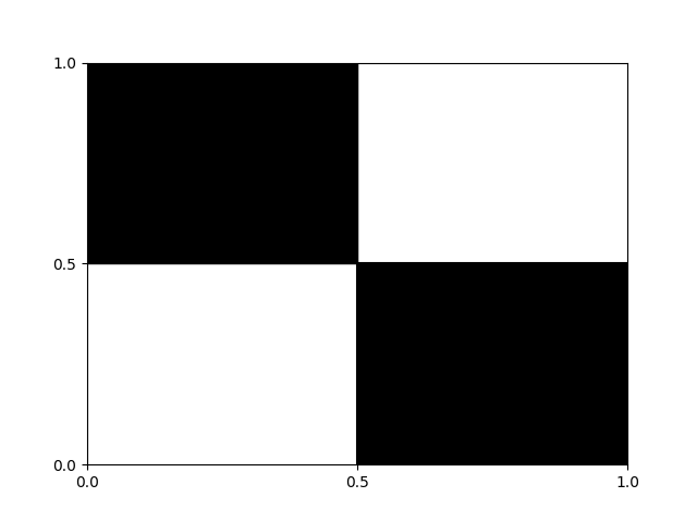
(a) Kernel $k$ defined in (16).

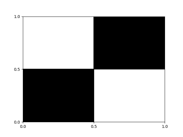
(b) Kernel $2\,k^{\otimes 2}$.

Figure 5. Support of some $\{0,1\}$-valued kernels.

For $A\subset\Omega$ measurable and $S$ be positive operators on $L^{p}$ with $p\in(1,+\infty)$, we denote by $S(A)$ the support (which is defined a.e.) of $Sf$, where $f\in L^{p}$ is any nonnegative function whose support is a.e. equal to $A$ (notice the support of $Sf$ is defined up to an a.e.  equivalence). More formally: the class $\mathcal{P}=\{B\in\mathcal{F}\,\colon\,k_{S}(B,A)=0\}$, where $k_{S}$ is defined in (8), is stable by countable union; thus Lemma 2.2 implies the existence of a maximal set for $\mathcal{P}$; then by definition its complementary is equal to $S(A)$. We now state some corresponding preliminary properties in the next two lemmas.

Lemma 3.43 (Basic properties of $T(A)$).

Let $T,S$ be positive operators on $L^{p}$ with $p\in(1,+\infty)$, and $A$ a measurable set. We have the following properties.

1. $\operatorname{supp}(T(f))=T(\operatorname{supp}(f))$ a.e. for any $f\in L^{p}_{+}$. In particular, if $\mathbb{1}_{A}$ belongs to $L^{p}$, then we have $T(A)=\operatorname{supp}(T(\mathbb{1}_{A}))$ a.e..

2. $T(S(A))=(TS)(A)$ a.e. and $(T+S)(A)=T(A)\cup S(A)$ a.e..

3. If $A\subset B$ a.e., with $B$ a measurable set, then we have $T(A)\subset T(B)$ a.e..

4. Let $(A_{i})_{i\in I}$ be an at most countable family of measurable sets. We have:

   $$T\left(\bigcup\limits_{i\in I}A_{i}\right)=\bigcup\limits_{i\in I}T(A_{i})\text{ a.e.}\quad\text{and}\quad T\left(\bigcap\limits_{i\in I}A_{i}\right)\subset\bigcap\limits_{i\in I}T(A_{i})\text{ a.e.}.$$

Proof.

Let $f^{\prime}\in L^{p}$ such that $f^{\prime}>0$ and $\mathbb{1}_{\operatorname{supp}(f)}f^{\prime}=f$. Then, by (7), we have for any measurable set $B$ that $k_{T}(B,\operatorname{supp}(f))=0$ if and only if $B\cap\operatorname{supp}\left(T\left(\mathbb{1}_{\operatorname{supp}(f)}f^{\prime}\right)\right)=\emptyset$. This gives Point i. Point ii is a direct consequence of Point i applied to $f\mathbb{1}_{A}$ for any positive function $f\in L^{p}$. Point iii is a direct consequence of the positivity of $T$.

We now prove Point iv. Let $B$ be a measurable set. As the map $k_{T}(B,.)$ is non-decreasing and $\sigma$-additive on $\mathcal{F}$, we have $k_{T}\left(B,\bigcup_{i\in I}A_{i}\right)=0$ if and only if for all $i\in I$, we have $k_{T}(B,A_{i})=0$. Thus the maximal set $B$ that satisfies $k_{T}\left(B,\bigcup_{i\in I}A_{i}\right)=0$ is $\bigcap_{i\in I}T(A_{i})^{c}$, that is, $T\left(\bigcup_{i\in I}A_{i}\right)=\bigcup_{i\in I}T(A_{i})$. The property $T\left(\bigcap_{i\in I}A_{i}\right)\subset\bigcap_{i\in I}T(A_{i})$ is a direct consequence of Point iii. We thus have Point iv. ∎

Lemma 3.44 ($T^{k}(A)$ and invariance/irreducibility).

Let $T$ be a positive operator on $L^{p}$ with $p\in(1,+\infty)$. Let $A$ be a measurable set, and $n\in\operatorname{\mathbb{N}}^{*}$. We have the following properties.

1. The set $A$ is $T$-invariant if and only if $T(A)\subset A$ a.e..

2. If the set $A$ is $T^{n}$-invariant, then for all $k\in\operatorname{\mathbb{N}}$, the set $T^{k}(A)$ is $T^{n}$-invariant.

3. If $T$ is a non-zero irreducible operator and $\mu(A)>0$, then we have $\mu(T(A))>0$. Moreover, we have $T(\Omega)=\Omega$ a.e..

Proof.

By definition the set $A$ is $T$-invariant if and only if $A^{c}\cap TA=\emptyset$; this gives Point i. Let the set $A$ be $T^{n}$-invariant and $k\in\operatorname{\mathbb{N}}$. Then by Lemma 3.43 ii, we have $T^{n}(T^{k}(A))=T^{k}(T^{n}(A))$. Since we have $T^{n}(A)\subset A$, we deduce that $T^{n}(T^{k}(A))\subset T^{k}(A)$. This gives Point ii.

Assume that $T$ is a non-zero irreducible operator and that $\mu(T(A))=0$. The latter condition implies that $A$ is $T$-invariant, and by irreducibility of $T$, that $A=\emptyset$ or $A=\Omega$. As $T$ is a non-zero operator, we get the latter case is impossible and thus we have $\mu(A)=0$. As the set $T(\Omega)$ is $T$-invariant with positive measure, we deduce that $T(\Omega)=\Omega$ by the previous argument. This gives Point iii. ∎

The following corollary provides an interesting link between the future of a set and the exponential of $T$.

Corollary 3.45 (Future and $\mathrm{e}^{T}$).

Let $T$ be a positive operator on $L^{p}$ with $p\in(1,+\infty)$ and $A$ a measurable set. We have:

$$\mathrm{e}^{T}(A)=\bigcup_{n\in\operatorname{\mathbb{N}}}T^{n}(A)=F(A)\quad\text{a.e.}.$$

Proof.

The first equality is elementary, using the same arguments as for Lemma 3.43 ii. We prove the second equality. The set $\bigcup_{n\in\operatorname{\mathbb{N}}}T^{n}(A)$ is clearly $T$-invariant by Lemma 3.44 i and contains $A$, we therefore have $F(A)\subset\bigcup_{n\in\operatorname{\mathbb{N}}}T^{n}(A)$. As $F(A)$ is a $T$-invariant set, it is a $T^{n}$-invariant set for any $n\in\operatorname{\mathbb{N}}$ by Lemma 3.5. We get that for any $n\in\operatorname{\mathbb{N}}$, $T^{n}(F(A))\subset F(A)$ by Lemma 3.44 i, and thus $\bigcup_{n\in\operatorname{\mathbb{N}}}T^{n}(A)\subset\bigcup_{n\in\operatorname{\mathbb{N}}}T^{n}(F(A))\subset F(A)$. This gives the second equality. ∎

We give the following result on the restriction of $T^{n}$ on a convex set.

Lemma 3.46 (Power of a restricted operator on a convex set).

Let $T$ be a positive operator on $L^{p}$ for $p\in(1,+\infty)$ and $A$ a convex set. Then we have $(T_{A})^{n}=(T^{n})_{A}$ for any $n\in\operatorname{\mathbb{N}}^{*}$.

For $n\in\operatorname{\mathbb{N}}^{*}$, we will thus use the notation $T^{n}_{A}$ for $(T_{A})^{n}=(T^{n})_{A}$ when $A$ is a convex set.

Proof.

Let $n\in\operatorname{\mathbb{N}}^{*}$. We have:

$$(T^{n})_{A}=M_{A}T^{n}M_{A}=M_{A}T^{n-1}M_{A}TM_{A}+M_{A}T^{n-1}M_{F^{*}(A)}TM_{A}=(T^{n-1})_{A}\,T_{A},$$

where we used that $T(A)\subset F(A)=A\cup F^{*}(A)$ for the second equality, and that $F^{*}(A)$ is $T$-invariant (as $A$ is convex, see Lemma 3.23) and thus $T^{n-1}$-invariant, so that $M_{A}T^{n-1}M_{F^{*}(A)}=0$ for the last. We conclude by iteration. ∎

The following result on the decomposition of atoms is also related to [25, Theorem 8] which states that the eigenvalues of $T$ (when $T$ is compact) whose modulus are equal to the spectral radius of $T$ are roots of unity. We say that a family of measurable sets $(A_{i})_{i\in I}$ forms an a.e. partition of a measurable set $B$ if we have: $A_{i}\cap A_{j}=\emptyset$ a.e.  for any $i\neq j$, and $B=\bigcup_{i\in I}A_{i}$ a.e..

Proposition 3.47 (Atoms of powers of $T$).

Let $T$ be a positive operator on $L^{p}$ with $p\in(1,+\infty)$ and $n\in\operatorname{\mathbb{N}}^{*}$. We have the following properties.

1. If $A$ is a $T^{n}$-atom, then there exists a $T$-atom $B$ such that $A\subset B$.

2. Let $B$ be a $T$-atom. There exists a $T^{n}$-atom $A\subset B$ and a divisor $\mathrm{d}$ of $n$ such that the family $(A_{k})_{0\leq k\leq\mathrm{d}-1}$, where $A_{k}=T^{k}(A)\cap B$, forms an a.e. partition of $A$ in $T^{n}$-atoms.

The second point is slightly more technical; its proof is given in the next section.

Proof of Point i.

Let $A$ be a $T^{n}$ atom. The family $\mathcal{P}=\{B\in\mathcal{A}(T)\,\colon\,A\subset B\}$ of measurable sets is clearly stable by countable intersection. Let $A^{\prime}$ denote a minimal set for $\mathcal{P}$, given by Lemma 2.2. Let $B\in\mathcal{A}(T)$ such that $B\subset A^{\prime}$. As $B\in\mathcal{A}(T^{n})$ by Lemma 3.39 i, we get that either $A\subset B$ or $A\cap B=\emptyset$. By the minimality of $A^{\prime}$, we deduce in the former case that $A^{\prime}=B$ and in the latter case that $A^{\prime}\cap B=\emptyset$, and thus $B=\emptyset$. This gives that $A^{\prime}$ is a $T$-atom which contains $A$. ∎

3.11. Proof of Proposition 3.47 ii

Thanks to Lemma 3.46 (with $A$ replaced by $B$), it is enough to consider the case where $\Omega$ is a $T$-atom, that is, $T$ is irreducible. The case $T=0$ being trivial, we shall assume in this section only that $T$ is a positive irreducible operator on $L^{p}$ for $p\in(1,+\infty)$ and $T\neq 0$. In particular, we have $T(\Omega)=\Omega$ a.e. (see Lemma 3.44 iii) and $F(A)=\Omega$ a.e.  for any measurable set $A$ with positive measure. Motivated by Corollary 3.45, we define, for any measurable set $A$ with positive measure, the quantity:

$$n_{A}=\inf\left\{m\in\operatorname{\mathbb{N}}^{*}\cup\{\infty\}\,\colon\,\bigcup_{j=0}^{m-1}T^{j}(A)=\Omega\quad\text{a.e.}\right\}.$$

If $A$ is a $T^{n}$ invariant set with positive measure, the set $\bigcup_{j=0}^{n-1}T^{j}A$ is $T$-invariant and contains $A$; by irreducibility it must be equal to $\Omega$, so $n_{A}\leq n$. It is also elementary to check that if $A\subset B$ a.e. for a measurable set $B$, then $n_{A}\geq n_{B}\geq 1$.

Let $\mathcal{I}_{n}^{*}$ be the family of $T^{n}$-invariant sets with positive measure. This set is non empty as it contains $\Omega$, and we have $n\geq n_{A}\geq 1$ for all $A\in\mathcal{I}^{*}_{n}$. We have the following technical properties.

Lemma 3.48 (Elementary properties).

Let $n\in\operatorname{\mathbb{N}}^{*}$ and $A\in\mathcal{I}^{*}_{n}$ (i.e., a non trivial $T^{n}$-invariant set).

1. Let $\ell\in\operatorname{\mathbb{N}}$. We have for $k\in\operatorname{\mathbb{N}}^{*}$:

   $$\bigcup_{j=\ell}^{k+\ell-1}T^{j}(A)=\Omega\quad\text{a.e.}\quad\Longleftrightarrow\quad n_{A}\leq k.$$

   In particular, we have $n_{T^{\ell}(A)}=n_{A}$.

2. Set $B=A\bigcap\left(\bigcup_{j=1}^{n_{A}-1}T^{j}(A)\right)$ (notice the indices $j$ are positive). We have:

   $$\mu(B)>0\quad\Longrightarrow\quad n_{B}>n_{A}.$$

Proof.

We prove Point i. The set $B=\bigcup_{j=0}^{k-1}T^{j}(A)$ is $T^{n}$-invariant as union of $T^{n}$-invariant sets, see Lemma 3.44 ii, and thus $T^{n}(B)\subset B$. If $T^{\ell}(B)=\Omega$, then we get, as $(\ell+1)n-\ell\geq 0$ and $T(\Omega)=\Omega$:

$$\Omega=T^{(\ell+1)n-\ell}(\Omega)=T^{(\ell+1)n}(B)\subset B,$$

and thus $B=\Omega$ and $n_{A}\leq k$. On the other hand, if $n_{A}\leq k$, then we have $B=\Omega$ and $T^{\ell}(B)=\Omega$.

We prove Point ii. The set $B=A\bigcap\left(\bigcup_{j=1}^{n_{A}-1}T^{j}(A)\right)$ is $T^{n}$-invariant, and thus belongs to $\mathcal{I}^{*}_{n}$ as $\mu(B)>0$. Using $B\subset A$ and thus $T^{j}(B)\subset T^{j}(A)$ for all the terms $j\geq 0$, we get:

$$\bigcup_{j=0}^{n_{A}-1}T^{j}(B)\subset\bigcup_{j=1}^{n_{A}-1}T^{j}(A).$$

By Point i (with $\ell=1$), the latter set is not a.e. equal to $\Omega$, which in turns, using Point i again (but with $\ell=0$), implies that $n_{B}>n_{A}$. ∎

Let $n\geq 2$. The supremum $n_{\max}=\sup\left\{n_{A}\,\colon\,A\in\mathcal{I}_{n}^{*}\right\}$ is less or equal than $n$ and is thus a maximum.

We can directly deduce Proposition 3.47 ii from the next lemma.

Lemma 3.49.

Let $A$ be a $T^{n}$-invariant set with positive measure such that $n_{A}=n_{\max}$. We have, with $A_{k}=T^{k}(A)$ for $k\in\operatorname{\mathbb{N}}$:

1. $n_{A}$ is a divisor of $n$.

2. $T^{n_{A}}(A_{k})=A_{k}$ a.e. for all $k\in\operatorname{\mathbb{N}}$.

3. $A_{k}\cap A_{\ell}=\emptyset$ a.e. for all $k\neq\ell$ in $\{0,\ldots,n_{A}-1\}$.

4. The sets $(A_{k})_{k\in\{0,\ldots n_{A}-1\}}$ are $T^{n}$-atoms.

Proof.

Let $A$ be $T^{n}$-invariant such that $n_{A}=n_{\max}$. Set $A^{*}_{k}=\bigcup_{j\in\{0,\ldots,n_{A}-1\}\setminus\{k\}}A_{j}$ for $k\in\{0,\ldots,n_{A}-1\}$ (so that $A_{k}\cup A_{k}^{*}=\Omega$ by definition of $n_{A}$) and $B=A\cap A^{*}_{0}$. The set $B$ is invariant. We assume that $\mu(B)>0$. Since $B\subset A$, we get $n_{B}\geq n_{A}$ and thus $n_{B}=n_{A}$ by maximality of $n_{A}$. Then, Lemma 3.48 ii implies that $\mu(B)=0$. By contradiction, we deduce that $\mu(B)=0$, that is:

$$A\cap A_{0}^{*}=\emptyset.$$

Using that $T(\Omega)=\Omega$ as $T$ is irreducible, we get:

$$A\sqcup A^{*}_{0}=\Omega=T(\Omega)=T^{n_{A}}(A)\cup A^{*}_{0}.$$

This implies that $A\subset T^{n_{A}}(A)$. Writing $n=kn_{A}+r$ with $r\in\{0,\ldots,n_{A}-1\}$, we get:

$$T^{r}(A)\subset T^{r+n_{A}}(A)\subset T^{r+kn_{A}}(A)=T^{n}(A)\subset A.$$

If $r>0$, this would imply that $n_{A}\leq r$. As $r<n_{A}$, we thus deduce that $r=0$, that is Point i, and then that $A=T^{n_{A}}(A)$. This gives Point ii for $k=0$ and thus for any $k$, as the $T^{n}$-invariant set $A_{k}$ is also maximal in the sense that $n_{A_{k}}=n_{A}=n_{\max}$ by Lemma 3.48 i.

Using again that $A_{k}$ is maximal and that $T^{n_{A}}(A_{j})=A_{j}$, we can apply the previous argument to get that $A_{k}\cap A^{*}_{k}=\emptyset$ for all $k\in\{0,\ldots,n_{A}-1\}$. This readily implies that the $A_{k}$ for $k\in\{0,\ldots,n_{A}-1\}$ are pairwise disjoint, that is, Point iii.

To conclude, it is enough to check Point iv for $k=0$. As $A$ is $T^{n}$-invariant, to prove it is a $T^{n}$-atom, it is enough to check that if $B\subset A$ is a $T^{n}$-invariant set with positive measure, then $B=A$. Consider such a set $B$. Notice that $n_{B}$ is finite (as $B\in\mathcal{I}^{*}_{n}$) and that $n_{B}\geq n_{A}$, that is $n_{B}=n_{A}$ by maximality of $n_{A}$. We thus have:

$$A\sqcup A^{*}_{0}=\Omega=B\bigcup\left(\bigcup_{j=1}^{n_{A}-1}T^{j}(B)\right)\,\subset\,B\cup A^{*}_{0}.$$

This readily implies that $A\subset B$ and thus $B=A$. ∎

4. Atoms and nonnegative eigenfunctions

Until the end of this section, $T$ is a power compact (that is, there exists $k\in\operatorname{\mathbb{N}}^{*}$ such that the operator $T^{k}$ is compact) positive operator on $L^{p}$, where $p\in(1,+\infty)$ and $(\Omega,\mathcal{F},\mu)$ is a measured space with $\mu$ $\sigma$-finite and non-zero. The purpose of this section is to study the intricate links between the ordered set of atoms and spectral properties of $T$. Especially, we study links between atoms and nonnegative eigenfunctions of $T$. We also provide some criteria of monatomicity of $T$. The power compactness hypothesis opens access to different results, giving the existence and uniqueness under irreducibility of nonnegative eigenfunctions for a positive operator.

4.1. On positive power compact operators

Recall that $\rho(T)$ defined in (1) denote the spectral radius of the operator $T$. The algebraic multiplicity of $\lambda\in\operatorname{\mathbb{C}}$ of $T$ is defined by:

(17) $$\operatorname{m}(\lambda,T)=\dim\left(\bigcup\limits_{k\in\operatorname{\mathbb{N}}^{*}}\mathrm{Ker}\,(T-\lambda\operatorname{Id})^{k}\right).$$

The complex number $\lambda\in\operatorname{\mathbb{C}}$ is an eigenvalue of $T$ when $\operatorname{m}(\lambda,T)\geq 1$, it is simple when $\operatorname{m}(\lambda,T)=1$. When $T$ is power compact, the multiplicity $\operatorname{m}(\lambda,T)$ is finite for $\lambda\in\operatorname{\mathbb{C}}^{*}$, see [18, Theorem p. 21]. Notice that for power compact operators the multiplicity of $\lambda\in\operatorname{\mathbb{C}}^{*}$ is also the dimension of the range of the spectral projection (which is the definition used in [25] and [11]) thanks to [11, Theorems VII.4.5-6].

For a measurable set $A\subset\Omega$, when there is no ambiguity on the operator $T$, we simply write $\rho(A)=\rho(T_{A})$, see Section 2.3, and $\operatorname{m}(\lambda,A)=\operatorname{m}(\lambda,T_{A})$ for the spectral radius and multiplicity of $\lambda$ for $T_{A}=M_{A}TM_{A}$, see (3), the operator $T$ restricted to $A$.

The following lemma proves that the restriction of a power compact operator is also power compact.

Lemma 4.1 (Restriction of a power compact operator).

Let $T$ be a positive power compact operator on $L^{p}$. Then there exists $k\in\operatorname{\mathbb{N}}^{*}$ such that for any measurable set $\Omega^{\prime}$, the operator $(T_{\Omega^{\prime}})^{k}$ is compact.

Proof.

Let $n\in\operatorname{\mathbb{N}}^{*}$ such that $T^{n}$ is compact. We have $0\leq(T_{\Omega^{\prime}})^{n}\leq T^{n}$. Since $T^{n}$ is compact, we get thanks to [3, Theorem 5.13] that $(T_{\Omega^{\prime}})^{3n}$ is compact. ∎

We say that the atom $A\subset\Omega$ is non-zero if $\rho(A)>0$, and denote by $\mathfrak{A}^{*}$ be the (at most countable) set of non-zero atoms:

(18) $$\mathfrak{A}^{*}=\{A\in\mathfrak{A}\,\colon\,\rho(A)>0\}.$$

Notice that $\operatorname{m}(\lambda,A)=0$ for all atoms $A\in\mathfrak{A}\setminus\mathfrak{A}^{*}$ and $\lambda\in\operatorname{\mathbb{C}}^{*}$.

We recall in our framework the classical results related to power compact operators.

Theorem 4.2.

Let $T$ be a positive power compact operator on $L^{p}$ with $p\in(1,+\infty)$.

1. Krein-Rutman. If $\rho(T)$ is positive then $\rho(T)$ is an eigenvalue of $T$, and there exists a corresponding nonnegative right eigenfunction denoted $v_{T}$.

2. de Pagter. If $T$ is irreducible then $\rho(T)$ is positive unless $T=0$ and $\dim(L^{p})=1$, that is, if $A$ is measurable then either $\mu(A)=0$ or $\mu(A^{c})=0$.

3. Perron-Jentzsch. If $T$ is irreducible with $\rho(T)>0$, then $\rho(T)$ is simple, $v_{T}$ is positive a.e., and $v_{T}$ is the unique nonnegative right eigenfunction of $T$.

4. Schwartz. We have for $\lambda\in\operatorname{\mathbb{C}}^{*}$:

   (19) $$\operatorname{m}(\lambda,T)=\sum_{A\in\mathfrak{A}^{*}}\operatorname{m}(\lambda,A)\quad\text{and}\quad\rho(T)=\max_{A\in\mathfrak{A}^{*}}\rho(A).$$

Remark 4.3.

In the Perron-Jentzsch result and in what follows, uniqueness of eigenfunctions is understood up to a multiplicative constant.

Proof.

We first recall the vocabulary used by Grobler [14]. For any $v\in L^{p}$, we denote by $E_{v}$ the smallest band (therefore the smallest subspace of the form $L^{p}_{A}$ with $A\in\mathcal{F}$) that contains $v$, that is $L^{p}_{\operatorname{supp}(v)}$. We say that $v\in L^{p}$ is quasi-interior if the closure of $E_{v}$ is equal to $L^{p}$, that is if $v>0\text{ a.e.}$.

Point i is given by [14, Theorem 3], and Point ii by [14, Theorem 12 (1)]. To prove Point iii, by [14, Theorem 12 (1)], since $T$ is irreducible, $\rho(T)$ is a simple eigenvalue and the corresponding eigenfunction is a quasi-interior point of $L^{p}$, that is a positive eigenfunction. By [24, Theorem 5.2 (iv), p. 329] (that can be applied as $T$ is power compact, see Corollary p. 329), $\rho(T)$ is the only eigenvalue related to a nonnegative eigenfunction. As $\rho(T)$ is simple, $v_{T}$ is the unique nonnegative eigenfunction of $T$.

Point 19 is an extension of [25, Theorem 7] (stated for $\mu$ finite and $T$ compact), and its proof is very similar. We provide a short proof for completeness. Let $h\in L^{1}$ with $1\geq h>0\text{ a.e.}$; thus the measure $h.\mu$, defined by $h.\mu(A)=\int_{A}h(s)\mu(\mathrm{d}s)$ for $A\in\mathcal{F}$, is finite. Following the proof of [25, Theorem 7], it is enough to check that Lemmas 4, 11 and 12 therein also hold by replacing $\mu$ by $h.\mu$ in their statement and when the operator $T$ is power compact.

For Lemma 11, the proof given by [25] is also valid when the operator $V$ given therein is power compact, as every point of $\operatorname{Sp}(V)\backslash\{0\}$ is isolated and as for any $\lambda\neq 0$, the quantity $\operatorname{m}(\lambda,V)$ is finite, see [11, Section VII.4]. For Lemma 12, the proof given by [25] holds for any positive operator, and also holds when we replace $\mu$ in the statement by the finite measure $h.\mu$.

Lemma 4 states that if $\mu$ is finite and $T$ is a positive compact operator, then for all $\lambda>0$ there exists $\delta>0$ such that for all measurable set $A\in\mathcal{F}$ such that $\mu(A)<\delta$ we have $\rho(T_{A})<\lambda$. An elementary adaptation of the proof of Lemma 4, gives that the result also holds if $\mu$ is $\sigma$-finite provided we replace the condition $\mu(A)<\delta$ by $h.\mu(A)<\delta$. We now assume that the operator $T$ is power compact, and let $k\in\operatorname{\mathbb{N}}^{*}$ be such that the operator $T^{k}$ is compact. For $\lambda>0$, there exists $\delta>0$ such that for all measurable set $A\in\mathcal{F}$ with $h.\mu(A)<\delta$ we have $\rho((T^{k})_{A})<\lambda^{k}$. Since $0\leq(T_{A})^{k}\leq(T^{k})_{A}$, we deduce that $\rho((T_{A})^{k})\leq\rho((T^{k})_{A})<\lambda^{k}$, that is $\rho(T_{A})<\lambda$ thanks to [18, Theorem p. 21]. This readily gives the extension of Lemma 4 to $\mu$ $\sigma$-finite and $T$ positive power compact. This concludes the proof of Point 19. ∎

Let us stress that Theorem 4.2 also applies to $T^{\star}$. Indeed, the operator $T$ is irreducible (resp. positive, resp. power compact) if and only if the operator $T^{\star}$ is irreducible (resp. positive, resp. power compact). By [18, Theorem p. 21], when $T$ is power compact, we have $\rho(T^{\star})=\rho(T)$ as well as $\operatorname{m}(\lambda,T^{\star})=\operatorname{m}(\lambda,T)$ for all $\lambda\in\operatorname{\mathbb{C}}^{*}$.

The following result is a direct consequence of Theorem 4.2, as any atom is irreducible by Theorem 3.34. The function $v_{A}$ below will be called the Perron-like eigenfunction of $T_{A}$.

Corollary 4.4 (Perron-like eigenfunctions for $T_{A}$).

Let $T$ be a positive power compact operator on $L^{p}$ with $p\in(1,+\infty)$ and $A$ a non-zero atom. Then $\rho(A)$ is a simple positive eigenvalue of $T_{A}$ and there exists a unique nonnegative right eigenfunction of $T_{A}$, say $v_{A}$; furthermore its support is $A$, that is, $\operatorname{supp}(v_{A})=A$ a.e., and we have $\rho(v_{A})=\rho(A)$: $T_{A}v_{A}=\rho(A)v_{A}$.

For $\lambda>0$, let $\mathfrak{A}(\lambda)$ be the set of atoms with spectral radius $\lambda$:

(20) $$\mathfrak{A}(\lambda)=\{A\in\mathfrak{A}^{*}\,\colon\,\rho(A)=\lambda\}.$$

We have the following elementary result, with the convention $\max\emptyset=0$.

Lemma 4.5 (Spectral radius of restricted operators).

Let $T$ be a positive power compact operator on $L^{p}$ with $p\in(1,+\infty)$.

1. For any $\lambda>0$, there exists a finite number of atoms with a spectral radius larger than $\lambda$.

2. If $\Omega^{\prime}$ is admissible, then we have:

   (21) $$\rho(\Omega^{\prime})=\max_{A\in\mathfrak{A}^{*},\,A\subset\Omega^{\prime}}\rho(A).$$

3. If $\rho(T)$ is positive, then we have $\operatorname{m}(\rho(T),T)=\operatorname{card}(\mathfrak{A}(\rho(T))$.

Proof.

By Corollary 4.4, any atom with a spectral radius $\rho(A)>0$ satisfies $\operatorname{m}(\rho(A),A)=1$. If $\lambda$ is positive, then by [11], the set $\{z\in\operatorname{\mathbb{C}},|z|\geq\lambda,\operatorname{m}(z,T)\neq 0\}$ is finite (notice that $\operatorname{m}(z,T)\in\operatorname{\mathbb{N}}$ by [18, Theorem p. 21]). Therefore, by Theorem 4.2 19, only a finite number of atoms $A$ may satisfy $\rho(A)\geq\lambda$, that is Point i. Point ii then follows from (19), since the atoms of $T_{\Omega^{\prime}}$ are precisely the atoms of $T$ that are included in $\Omega^{\prime}$, by Proposition 3.32 ii.

Finally, for any atom $A$, we have $\rho(A)\leq\rho(T)$, therefore the only atoms with $\operatorname{m}(\rho(T),A)>0$ are exactly those with $\rho(A)=\rho(T)$. By Corollary 4.4, these atoms satisfy $\operatorname{m}(\lambda,A)=1$, thus we deduce Point iii from (19). ∎

We directly deduce from ii the following result.

Lemma 4.6 (The operator is quasi-nilpotent outside the non-zero atoms).

The restriction $T_{\Omega^{\prime}}$ of $T$ to $\Omega^{\prime}$, the complement set of $\bigcup_{A\in\mathfrak{A}^{*}}A$, is quasi-nilpotent, that is, $\rho(\Omega^{\prime})=0$.

4.2. Nonnegative eigenfunctions

The goal of this section is to describe exactly the set of nonnegative eigenfunctions and prove Theorem 3. We start by two elementary results.

Lemma 4.7.

If $C$ is convex, and $\operatorname{supp}(v)\subset F(C)$, then we have $T_{C}v=\mathbb{1}_{C}Tv$.

Proof.

Since $C$ is convex, $F(C)=C\sqcup F^{*}(C)$ where $F^{*}(C)$ is invariant by Lemma 3.23. Since $\operatorname{supp}(v)\subset F(C)$, we have $v=v\mathbb{1}_{C}+v\mathbb{1}_{F^{*}(C)}$. The statement follows by checking that, by Lemma 3.3, $\mathbb{1}_{C}T(v\mathbb{1}_{F^{*}(C)})=0$. ∎

Lemma 4.8 (Nonnegative eigenfunctions on an atom).

Let $T$ be a positive operator on $L^{p}$ for $p\in(1,+\infty)$ and $A$ a non-zero atom. If $v$ is a nonnegative right eigenfunction with $A\subset\operatorname{supp}(v)\subset F(A)$, then $v$ coincides on $A$ with the Perron like right eigenfunction: $\mathbb{1}_{A}v=\mathrm{c}v_{A}$ for some $\mathrm{c}>0$, and $\rho(v)=\rho(A)$, that is, $Tv=\rho(A)v$.

Proof.

Let $\lambda\geq 0$ with $Tv=\lambda v$. Since $\operatorname{supp}(v)\subset F(A)$, we may apply Lemma 4.7 to the atom $A$, which is convex by Theorem 3.34, to get $T_{A}(\mathbb{1}_{A}v)=T_{A}v=\mathbb{1}_{A}Tv=\lambda\mathbb{1}_{A}v,$ that is, $\mathbb{1}_{A}v$ is a nonnegative eigenfunction of $T_{A}$. Since $A\subset\operatorname{supp}(v)$, we get $\mathbb{1}_{A}v$ is non-zero. By Corollary 4.4, we have $\lambda=\rho(A)$ and $\mathbb{1}_{A}v=\mathrm{c}v_{A}$ for some $\mathrm{c}>0$, as claimed. ∎

We need an adaptation of [20, Theorem 4], a result originally stated for kernel operators, and which concerns subsolutions to the eigenvalue equation, that is, functions $f$ that satisfy:

(22) $$Tf\leq\lambda f.$$

Proposition 4.9 (Nelson: Nonnegative subsolutions are Perron eigenfunctions).

Let $T$ be a positive power compact irreducible operator on $L^{p}$ with $p\in(1,+\infty)$. If $f\in L^{p}_{+}$ satisfies (22) for some $\lambda\in(0,\rho(T)]$, then we have $Tf=\rho(T)f$.

Proof.

Let $f\in L^{p}_{+}$ be a solution of (22). Without loss of generality we may assume $\lambda=\rho(T)$. By the Perron-Jentzch theorem (Theorem 4.2 iii), there exists a nonnegative left eigenfunction $h\in L^{q}_{+}$ with left eigenvalue $\rho(T)$ such that $h>0$ a.e.. Taking the bracket of (22) with the nonnegative function $h$, and using the fact that it is a left eigenfunction of $T$, we get:

$$\rho(T)\langle h,f\rangle=\langle h,Tf\rangle\leq\langle h,\rho(T)f\rangle=\rho(T)\langle h,f\rangle,$$

where the inequality holds by positivity of $T$ and nonnegativity of $f$ and $h$. Therefore we have $\langle h,Tf\rangle=\langle h,\rho(T)f\rangle$, so $\langle h,\rho(T)f-Tf\rangle=0$. Since $\rho(T)f-Tf$ is nonnegative and $h>0\text{ a.e.}$, this implies $Tf=\rho(T)f$. ∎

As a first consequence, we give details on which atoms may appear in the support of a nonnegative eigenfunction. Recall that, for a non-zero atom $A$, the Perron like eigenfunction $v_{A}$ is the right eigenfunction of $T_{A}$ given by Corollary 4.4. For $v\in L^{p}_{+}$ a nonnegative eigenfunction of $T$, we consider the following subset of the atoms $\mathfrak{A}(\rho(v))$:

$$\mathfrak{A}_{m}(v):=\{A\in\mathfrak{A}\,\colon\,A\subset\operatorname{supp}(v)\quad\text{and}\quad\rho(v)=\rho(A)\}.$$

Corollary 4.10 (A dichotomy for atoms and nonnegative eigenfunctions).

Let $T$ be a positive power compact operator on $L^{p}$ with $p\in(1,+\infty)$. Let $v\in L^{p}_{+}$ be a nonnegative eigenfunction of $T$ with $\lambda=\rho(v)>0$.

1. For any atom $A$ with $A\subset\operatorname{supp}(v)$ a.e., exactly one of the following holds:

   • $\rho(A)<\lambda$ ;

   • $\rho(A)=\lambda$, that is, $A\in\mathfrak{A}_{m}(v)$, $\mathbb{1}_{A}v=\mathrm{c}v_{A}$ for some $\mathrm{c}>0$ and $\operatorname{supp}(v)\cap P^{*}(A)=\emptyset$ a.e..

2. The set of atoms $\mathfrak{A}_{m}(v)$ is a nonempty finite antichain, and:

   $$\rho(v)=\rho(\operatorname{supp}(v)).$$

3. If $A\in\mathfrak{A}_{m}(v)$, $B\in\mathfrak{A}$ and $B\prec A$, then we have $\rho(B)<\rho(A)$.

Proof.

We start by proving i. Let $v$, $\lambda$ satisfy the hypotheses, and consider an atom $A$ such that $A\subset\operatorname{supp}(v)$. If $\rho(A)<\lambda$ we are in the first case and there is nothing to prove. We now assume $\lambda\leq\rho(A)$. Since $T$ is a positive operator and $v$ is nonnegative, we have:

(23) $$T_{A}(v\mathbb{1}_{A})=\mathbb{1}_{A}T(v\mathbb{1}_{A})\leq\mathbb{1}_{A}T(v\mathbb{1}_{A})+\mathbb{1}_{A}T(v\mathbb{1}_{A^{c}})=\mathbb{1}_{A}Tv=\lambda\mathbb{1}_{A}v.$$

Since $\lambda\leq\rho(A)$, and $A$ is irreducible, Proposition 4.9 applied to $T_{|A}$ implies $T_{A}v_{A}=\rho(A)v_{A}$. Since we have $A\subset\operatorname{supp}(v)$, $v_{A}$ is not the zero function, thus, by Corollary 4.4, we have $\lambda=\rho(A)$ and $\mathbb{1}_{A}v=\mathrm{c}v_{A}$ for some $\mathrm{c}>0$. Going back to (23), we see that the inequality there is in fact an equality, so $\mathbb{1}_{A}T(v\mathbb{1}_{A^{c}})=0$. By (7), we thus have $k_{T}(A,\operatorname{supp}(v)\cap A^{c})=0$. By Lemma 3.6, the set $\operatorname{supp}(v)$ is invariant, thus by additivity of the kernel we also have:

$$k_{T}(A\cup\operatorname{supp}(v)^{c},\operatorname{supp}(v)\cap A^{c})=0,$$

so that $\operatorname{supp}(v)\cap A^{c}$ is invariant. We then write $F(\operatorname{supp}(v)\cap A^{c})\cap A=(\operatorname{supp}(v)\cap A^{c})\cap A=\emptyset,$ which implies by Lemma 3.14 that:

(24) $$\operatorname{supp}(v)\cap P^{*}(A)=\operatorname{supp}(v)\cap A^{c}\cap P(A)=\emptyset.$$

This completes the proof of Point i

We now turn to the proof of ii. If two atoms $A$ and $B$ are in $\mathfrak{A}_{m}(v)$, Equation (24) shows that $B$ cannot be a subset of $P^{*}(A)$; symmetrically $A$ cannot be included in $P^{*}(B)$. By the alternate formulation of $\preccurlyeq$ from Lemma 3.37, $A$ and $B$ are not comparable, so $\mathfrak{A}_{m}(v)$ is an antichain. It is finite by Lemma 4.5 i. Moreover, as $T(v)=\lambda v$, we get that $T_{\operatorname{supp}(v)}(v)=\lambda v$, and thus $\rho(\operatorname{supp}(v))\geq\lambda$. As the set $\operatorname{supp}(v)$ is invariant by Lemma 3.6 (and thus admissible), by (21), there exists an atom $A\subset\operatorname{supp}(v)$ with $\rho(A)\geq\lambda$, and thus $\rho(A)=\lambda$ by Point i. This implies that the finite antichain $\mathfrak{A}_{m}(v)$ is not empty.

Finally, if $A\in\mathfrak{A}_{m}(v)$ and $B\prec A$, then we get $B\subset F(A)\subset\operatorname{supp}(v)$ since $\operatorname{supp}(v)$ is invariant. Applying the dichotomy from Point i, and noting that $B$ cannot be in $\mathfrak{A}_{m}(v)$ since it is an antichain, we deduce that $\rho(B)<\rho(A)=\lambda$. ∎

The last statement of Corollary 4.10 motivate the following definition, we refer to Figure 6 for a pictorial representation.

Definition 4.11 (Distinguished atoms and eigenvalues).

Let $T$ be a positive power compact operator on $L^{p}$ with $p\in(1,+\infty)$. A non-zero atom $A$ of $T$ is called right distinguished if $\rho(B)<\rho(A)$ for any atom $B$ such that $B\prec A$.

The set of right distinguished atoms of radius $\lambda>0$ is denoted by $\mathfrak{A}_{\mathrm{dist}}(\lambda)$.

An eigenvalue $\lambda$ is called right distinguished if $\mathfrak{A}_{\mathrm{dist}}(\lambda)\neq\emptyset$.

One has a similar definition for left distinguished atoms/eigenvalues. When there is no ambiguity, we shall simply write distinguished for right distinguished.

By Corollary 4.10 ii, if $v$ is a nonnegative eigenvalue, all atoms in $\mathfrak{A}_{m}(v)$ are distinguished:

(25) $$\mathfrak{A}_{m}(v)\subset\mathfrak{A}_{\mathrm{dist}}.$$

In the other direction, we now show that for any distinguished atom, we may associate a nonnegative eigenfunction. Recall that, for a non-zero atom $A$, $v_{A}$ denotes the Perron-like eigenfunction of $T_{A}$ given by Corollary 4.4.

Proposition 4.12 (Nonnegative eigenfunctions associated to distinguished atoms).

Let $T$ be a positive power compact operator on $L^{p}$ with $p\in(1,+\infty)$, and $A$ a non-zero atom. The following statements are equivalent:

1. $A$ is a distinguished atom.

2. $\rho(F^{*}(A))<\rho(A)$.

3. There exists a nonnegative eigenfunction $w_{A}\in L^{p}_{+}$ such that $\operatorname{supp}(w_{A})=F(A)$ and $\mathbb{1}_{A}w_{A}=v_{A}$.

If they hold, then we have $\rho(w_{A})=\rho(A)$.

The condition $\mathbb{1}_{A}w_{A}=v_{A}$ in iii corresponds to a particular choice of normalizing constant, see Lemma 4.8.

Diagram of the ordered set of atoms. Following the classical convention (see [6, p. 4]), each circle represents an atom $A$, and is labeled with its radius $\rho(A)$. An arrow from atom $A$ to atom $B$ signifies that $B\prec A$ and there is no atom in between.

The distinguished atoms are those circled in a thick line.

Note that a family of similar “finite” pictures may always be drawn in the general case, by considering only atoms with radius larger than a positive constant $\lambda$.

Figure 6. Distinguished atoms

Proof.

Suppose that Point iii holds, and let $w_{A}$ be a nonnegative eigenfunction with $\operatorname{supp}(w_{A})=F(A)$. By Lemma 4.8, we have $\rho(w_{A})=\rho(A)$, so $A\in\mathfrak{A}_{m}(w_{A})$, and by (25), it is distinguished. Therefore Point iii implies Point i.

Suppose that Point i holds. By (21), either $\rho(F^{*}(A))=0$, or there exists an atom $B\subset F^{*}(A)$ such that $\rho(F^{*}(A))=\rho(B)$. By Lemma 3.37, this $B$ satisfies $B\prec A$. Since $A$ is distinguished, $\rho(B)<\rho(A)$, so Point ii holds.

We now prove that Point ii implies Point iii. Set $B=F^{*}(A)$. By assumption, the invariant set $B$ satisfies $\rho(B)<\rho(A)$. By Lemma 3.7, the operator $(\rho(A)\operatorname{Id}-T_{B})$ is invertible and its inverse is a positive operator. Let $w_{A}=v_{A}+f_{B}$, where $f_{B}=(\rho(A)\operatorname{Id}-T_{B})^{-1}(\mathbb{1}_{B}Tv_{A})$. Note that, by the expression of $(\rho(A)\operatorname{Id}-T_{B})^{-1}$ as a Neumann series, we have $\operatorname{supp}(f_{B})\subset B$, and thus $\mathbb{1}_{A}w_{A}=v_{A}$. Then we have:

(26) $$Tw_{A}=Tv_{A}+Tf_{B}=\mathbb{1}_{A}Tv_{A}+\mathbb{1}_{A^{c}}Tv_{A}+Tf_{B}.$$

As $\operatorname{supp}(f_{B})$ is a subset of the invariant set $B$, we know by Lemma 3.3 that $Tf_{B}=T_{B}f_{B}$. Moreover, as $\operatorname{supp}(v_{A})\subset A$, we have $\mathbb{1}_{A}Tv_{A}=T_{A}v_{A}=\rho(A)v_{A}$ by definition of $v_{A}$. Finally, as the set $F(A)$ is invariant and as we have $\operatorname{supp}(v_{A})\subset A\subset F(A)$, we have $\mathbb{1}_{F(A)^{c}}Tv_{A}=0$, thus $\mathbb{1}_{A^{c}}Tv_{A}=\mathbb{1}_{B}Tv_{A}$. Plugging this in (26) yields:

$$Tw_{A} =\rho(A)v_{A}+\mathbb{1}_{B}Tv_{A}+\rho(A)f_{B}-\rho(A)f_{B}+T_{B}f_{B}$$

$$=\rho(A)w_{A}+\mathbb{1}_{B}Tv_{A}-(\rho(A)\operatorname{Id}-T_{B})(f_{B})$$

$$=\rho(A)w_{A}$$

by definition of $f_{B}$. So $w_{A}$ is a nonnegative eigenfunction (with $\rho(w_{A})=\rho(A)$). In particular, $\operatorname{supp}(w_{A})$ is an invariant set that contains $A$, so $F(A)\subset\operatorname{supp}(w_{A})$. Since $\operatorname{supp}(v_{A})$ and $\operatorname{supp}(f_{B})\subset B$ are both subsets of $F(A)$, we get $F(A)=\operatorname{supp}(w_{A})$. This proves Point iii. ∎

The previous result shows that, to any distinguished $\lambda$, we may associate a family $(w_{A})_{A\in\mathfrak{A}_{\mathrm{dist}}(\lambda)}$ composed of nonnegative eigenfunctions. We now completely describe the set of nonnegative eigenfunctions associated to $\lambda$, say $V_{+}(\lambda)$, as the conical hull of this family (that is linear combinations with nonnegative coefficients).

Theorem 4.13 (Characterization of nonnegative right eigenfunctions).

Let $T$ be a positive power compact operator on $L^{p}$ with $p\in(1,+\infty)$. Let $\lambda>0$. We have the following properties.

1. There exists a nonnegative eigenfunction of $T$ associated to $\lambda$ if and only if $\lambda$ is a distinguished eigenvalue.

2. The set $\mathfrak{A}_{\mathrm{dist}}(\lambda)$ is a (possibly empty) finite antichain of atoms, and the family $(w_{A})_{A\in\mathfrak{A}_{\mathrm{dist}}(\lambda)}$ is linearly independent.

3. If $v$ is a nonnegative eigenfunction with $\rho(v)=\lambda$, then $\lambda=\rho(\operatorname{supp}(v))$ and:

   $$v=\sum_{A\in\mathfrak{A}_{m}(v)}\mathrm{c}_{A}w_{A}\quad\text{with}\quad\mathrm{c}_{A}>0.$$

   So the cone $V_{+}(\lambda)$ is the conical hull of $\{w_{A}\,\colon\,A\in\mathfrak{A}_{\mathrm{dist}}(\lambda)\}$.

Remark 4.14.

The last point shows in particular that if $w$ is a nonnegative eigenfunction such that $\operatorname{supp}(w)=F(A)$, where $A$ is a non-zero atom (see Lemmas 3.6 and 4.8), then $A$ is distinguished, $\rho(w)=\rho(\operatorname{supp}(w))=\rho(A)$ and $w=\mathrm{c}w_{A}$ with $\mathrm{c}>0$.

The elementary adaptation of the theorem to nonnegative left eigenfunction is left to the reader.

Proof.

If $\lambda$ is distinguished, then by definition there is an atom $A\in\mathfrak{A}_{\mathrm{dist}}(\lambda)$, and $w_{A}$ provides a nonnegative eigenfunction associated to $\lambda$. Conversely, if there is a nonnegative eigenfunction $w$ associated to $\lambda$, then $\mathfrak{A}_{m}(w)$ is nonempty and consists of distinguished atoms by Corollary 4.10, so $\lambda$ is distinguished. This proves Point i.

Let us prove Point ii. If $A$ and $B$ belongs to $\mathfrak{A}_{\mathrm{dist}}(\lambda)$, then $\rho(A)=\rho(B)$, so they are not comparable by definition of distinguished atoms. Therefore $\mathfrak{A}_{\mathrm{dist}}(\lambda)$ is an antichain. It is also finite by Lemma  4.5 i. To prove the linear independence property, assume that $\sum_{B\in\mathfrak{A}_{\mathrm{dist}}(\lambda)}\mathrm{c}_{B}w_{B}=0$. Multiplying by $\mathbb{1}_{A}$ for $A\in\mathfrak{A}_{\mathrm{dist}}(\lambda)$ yields $\mathrm{c}_{A}v_{A}=0$, since for $B\neq A$, $\operatorname{supp}(w_{B})=F(B)$ is disjoint from $A$. Since $v_{A}$ is positive, $\mathrm{c}_{A}=0$. Since this is true for all $A$, the family $(w_{A})_{A\in\mathfrak{A}_{\mathrm{dist}}(\lambda)}$ is linearly independent.

We now prove Point iii. Since the $w_{A}$ are all in the cone $V_{+}(\lambda)$, their conical hull is included in $V_{+}(\lambda)$, so that we only need to prove the reverse inclusion. Let $v\in V_{+}(\lambda)$. By Corollary 4.10, there is an antichain $\mathfrak{A}_{m}(v)\subset\mathfrak{A}_{\mathrm{dist}}(\lambda)$ of distinguished atoms of radius $\lambda$ in the support of $w$, and all other atoms in this support satisfy $\rho(B)<\lambda$. Define:

$$B=\operatorname{supp}(v)\bigcap\bigg{(}\bigcup_{A\in\mathfrak{A}_{m}(v)}P(A)\bigg{)}^{c}=\operatorname{supp}(v)\bigcap\bigg{(}\bigcup_{A\in\mathfrak{A}_{m}(v)}A\bigg{)}^{c},$$

where the second equality follows from the fact that $\operatorname{supp}(v)\cap P^{*}(A)=\emptyset$ for all $A\in\mathfrak{A}_{m}(v)$, by Corollary 4.10. The first equality shows that $B$ is invariant.

Still following Corollary 4.10, there exist $\mathrm{c}_{A}>0$ such that $v\mathbb{1}_{A}=\mathrm{c}_{A}v_{A}$ for $A\in\mathfrak{A}_{m}(v)$. Consider the function $w=v-\sum_{A\in\mathfrak{A}_{m}(v)}\mathrm{c}_{A}w_{A}$. Since $\operatorname{supp}(w_{A})=F(A)\subset\operatorname{supp}(v)$, $\operatorname{supp}(w)$ is included in $\operatorname{supp}(v)$. Since $w$ vanishes by construction on all atoms $A\in\mathfrak{A}_{m}(v)$, we have in fact $\operatorname{supp}(w)\subset B$. Now, $Tw=\lambda w$ since $v$ and the $w_{A}$ are eigenfunctions. Since $B$ is invariant and $\operatorname{supp}(w)\subset B$, we get that $T_{B}w=\lambda w$. However, by construction, $B$ cannot contain atoms of radius greater than or equal to $\lambda$, so $\rho(B)<\lambda$. Therefore $\lambda$ cannot be an eigenvalue of $T_{B}$, and $w$ must be identically zero, so that $v=\sum_{A\in\mathfrak{A}_{m}(v)}\mathrm{c}_{A}w_{A}$. Since $\mathfrak{A}_{m}(v)\subset\mathfrak{A}_{\mathrm{dist}}(\lambda)$, we get that $v$ is in the conical hull of the $(w_{A})_{A\in\mathfrak{A}_{\mathrm{dist}}}$. This finishes the proof. ∎

4.3. Monatomic operators: definition and characterization

In this section we shall consider positive power compact operators having only one non-zero atom, which are called monatomic operators ($T$ is monatomic if $\operatorname{card}\mathfrak{A}^{*}=1$ with $\mathfrak{A}^{*}$ defined in (18)). We give in the next theorem a characterization of the monatomic positive power compact operators, see Theorem 2.

Theorem 4.15 (Characterization of monatomic operators).

Let $T$ be a positive power compact operator on $L^{p}$ with $p\in(1,+\infty)$ such that $\rho(T)>0$. The following properties are equivalent.

1. The operator $T$ is monatomic.

2. There exist a unique right and a unique left nonnegative eigenfunctions of $T$ with non-zero eigenvalues, and $\rho(T)$ is a simple eigenvalue of $T$.

3. There exist a unique right and a unique left nonnegative eigenfunctions of $T$ with non-zero eigenvalues, say $u$ and $v$, and $\operatorname{supp}(u)\cap\operatorname{supp}(v)$ has positive measure.

Furthermore, when the operator $T$ is monatomic, we have $\rho(u)=\rho(v)=\rho(T)$ and $\operatorname{supp}(u)\cap\operatorname{supp}(v)$ is the non-zero atom of $T$.

(a) Graph associated to a kernel operator

$\begin{pmatrix}1&0\\ 1&1\\ \end{pmatrix}$

(b) Matrix associated to a kernel operator

Figure 7. Example of associated graph and associated matrix of a kernel operator on $\Omega=\{1,2\}$

Example 4.16 (On the condition $\rho(T)$ simple and $\operatorname{supp}(u)\cap\operatorname{supp}(v)$ with positive measure).

If $T$ has a unique right and a unique left eigenfunction, then $T$ is not monatomic in general. Indeed, consider the example given by Fig. 7 with $\Omega=\{1,2\}$ endowed with the counting measure. The positive kernel operator $T$ associated to the matrix given in Fig. 7(b) has only one right eigenfunction $u=(0,1)$ and one left eigenfunction $v=(1,0)$, but it is not monatomic, as its non-zero atoms are $\{1\}$ and $\{2\}$. Here, we have $\operatorname{supp}(u)\cap\operatorname{supp}(v)=\emptyset$ and $\rho(T)=1$ is not a simple eigenvalue.

To prove Theorem 4.15, we use the following lemma.

Lemma 4.17 (Existence of minimal distinguished atoms).

Let $A$ be a non-zero atom. Then there exists a right (resp. left) distinguished atom smaller (resp. larger) than $A$ for $\preccurlyeq$, say $B$, such that $\rho(B)\geq\rho(A)$.

Proof.

Recall that $T$ and $T^{\star}$ have the same spectral radius and that they share the same atoms, so we only need to prove the lemma for right distinguished atoms for $T$, as it will then hold for left distinguished atoms for $T$ as they are right distinguished atoms for $T^{\star}$.

Since $A$ is a non-zero atom, $\rho(A)$ is positive. The set:

$$\mathcal{A}=\{C\in\mathfrak{A}^{*}\,\colon\,\rho(C)\geq\rho(A),C\preccurlyeq A\}$$

is finite thanks to Lemma 4.5 i and is non empty as it contains $A$. Thus it has at least one minimal element for the order $\preccurlyeq$, say $B$. If an atom $C$ satisfies $C\prec B$, then $C\preccurlyeq A$ by transitivity, but $C$ cannot be in $\mathcal{A}$ by minimality of $B$, so $\rho(C)<\rho(A)$. Since $B\in\mathcal{A}$, we have $\rho(B)\geq\rho(A)$, and so $\rho(C)<\rho(B)$. Since this holds for any $C$ such that $C\prec B$, we obtain the atom $B$ is distinguished. ∎

Proof of Theorem 4.15.

We assume that $T$ is monatomic and prove Point ii. Let $A$ be the only non-zero atom. By Lemma 4.5 iii, as $\operatorname{m}(\rho(T),T)\geq 1$ and $\mathfrak{A}^{*}$ is reduced to $\{A\}$, we get that $\rho(T)$ is simple and $\rho(A)=\rho(T)$ by (21).

We now prove the existence and uniqueness of a nonnegative right eigenfunction. Since there is no other non-zero atom, using directly Definition 4.11 we see that $A$ is distinguished, and is the only distinguished atom. Still by definition, $\rho(A)$ is the only distinguished eigenvalue. By Theorem 4.13, the set of nonnegative eigenfunctions is the cone $\mathbb{R}_{+}w_{A}$, which proves uniqueness (up to a positive multiplicative constant). Applying the same proof to $T^{\star}$ gives Point ii and the first part of the last sentence of the theorem.

We assume Point ii and prove Point iii. Since $\rho(T)>0$ is simple, we deduce from (19) that there exists a unique atom, say $A$, such that $\rho(A)=\rho(T)$. In particular, all other atoms must satisfy $\rho(B)<\rho(A)$, so that $A$ is right (and left) distinguished. Therefore, by Proposition 4.12, the unique right (resp. left) nonnegative eigenfunction, whose existence is given by our Assumption, is in fact $w_{A}$ (resp. the nonnegative eigenfunction $w_{A}^{\star}$ obtained from $T^{\star}$). Since $\operatorname{supp}(w_{A})\cap\operatorname{supp}(w_{A}^{\star})=F(A)\cap P(A)=A$ by convexity of the atom $A$, we obtain Point iii and the last part of the last sentence of the theorem.

We assume Point iii and prove that the operator $T$ is monatomic. Since $\rho(T)>0$, there exists an atom, say $A$, such that $\rho(A)=\rho(T)$. Looking for a contradiction, we assume there exists an other non-zero atom $B$ and without loss of generality that it is not smaller than $B$ for $\preccurlyeq$ (that is, either $A\preccurlyeq B$ or $A$ and $B$ are not comparable), equivalently $F(A)\cap B=\emptyset$. By Lemma 3.14, this is also equivalent to $F(A)\cap P(B)=\emptyset$.

Then, using Lemma 4.17, there exists a right (resp. left) distinguished atom $A^{\prime}$ (resp. $B^{\prime}$) such that $A^{\prime}\preccurlyeq A$ (resp. $B\preccurlyeq B^{\prime}$). By Proposition 4.12, the unique non negative right eigenfunction $v$ must satisfy $\operatorname{supp}(v)=F(A^{\prime})$, and similarly the unique non negative left eigenfunction $u$ must satisfy $\operatorname{supp}(u)=P(B^{\prime})$. By construction, we have $F(A^{\prime})\subset F(A)$ and $P(B^{\prime})\subset P(B)$, and thus $\operatorname{supp}(v)\cap\operatorname{supp}(u)=F(A^{\prime})\cap P(B^{\prime})\subset F(A)\cap P(B)=\emptyset$. As this is in contradiction with the assumption of Point iii, we deduce that $A$ is the only non-zero atom, that is $T$ is monatomic. ∎

5. Generalized eigenspace at the spectral radius

5.1. Framework and main theorem

The purpose of this section is to restate [17, Theorem V.1 (2)] on the ascent of $T$ in our framework of $L^{p}$-spaces, with a shorter proof based on convex sets.

Let us first recall a few classical definitions, see [11] and [18]. For $T$ an bounded operator on a Banach space and $\lambda\in\operatorname{\mathbb{C}}$, we call generalized eigenspace of $T$ at $\lambda$, and denote by $K(\lambda,T)$, the linear subspace:

$$K(\lambda,T)=\bigcup\limits_{k\in\operatorname{\mathbb{N}}}\mathrm{Ker}\,(T-\lambda\operatorname{Id})^{k}.$$

We now focus on the spectral radius $\lambda=\rho(T)$, and write $K(T)=K(\rho(T),T)$ the corresponding generalized eigenspace. We define the index of a generalized eigenvector $u\in K(T)$, as $\inf\{k\in\operatorname{\mathbb{N}}\,\colon\,u\in\mathrm{Ker}\,(T-\rho(T)\operatorname{Id})^{k}\}$, and, with the convention $\inf\emptyset=+\infty$, the ascent of $T$ at $\rho(T)$ as:

$$\alpha_{T}=\inf\{k\in\operatorname{\mathbb{N}}:\mathrm{Ker}\,(T-\rho(T)\operatorname{Id})^{k}=\mathrm{Ker}\,(T-\rho(T)\operatorname{Id})^{k+1}\}.$$

Notice that $\alpha_{T}$ is positive if $\rho(T)$ is an eigenvalue and that $K(T)=\mathrm{Ker}\,(T-\rho(T)\operatorname{Id})^{\alpha_{T}}$ when $\alpha_{T}$ is finite. When the operator $T$ is power compact, then the ascent $\alpha_{T}$ is finite, see [18, Lemma 1.a.2, Theorem p. 21] (it is also equal to the descent $\delta_{T}=\inf\{k\in\operatorname{\mathbb{N}}:\operatorname{Im}(T-\rho(T)\operatorname{Id})^{k}=\operatorname{Im}(T-\rho(T)\operatorname{Id})^{k+1}\}$).

Let $T$ be a positive power compact operator on $L^{p}$ with $p\in(1,+\infty)$, and assume $\rho(T)>0$, and thus $\alpha_{T}\in\operatorname{\mathbb{N}}^{*}$. By Lemma 4.5 iii, $K(T)$ is finite dimensional, and:

$$\dim(K(T))=m(\rho(T),T)=\operatorname{card}({\mathfrak{A}_{\mathrm{crit}}}),$$

where ${\mathfrak{A}_{\mathrm{crit}}}$ is the set of critical atoms:

(27) $${\mathfrak{A}_{\mathrm{crit}}}=\{A\in\mathfrak{A}\,\colon\,\rho(A)=\rho(T)\}.$$

By definition of $\alpha_{T}$, the sequence $(\dim(\mathrm{Ker}\,((T-\rho(T)\operatorname{Id})^{k})))_{1\leq k\leq\alpha_{T}}$ is (strictly) increasing, so we have the following trivial bounds:

(28) $$\dim\left(\mathrm{Ker}\,(T-\rho(T)\operatorname{Id})^{k}\right)\geq k,\quad\text{for all}\quad 1\leq k\leq\alpha_{T},$$

and in particular $\dim(K(T))=\operatorname{card}({\mathfrak{A}_{\mathrm{crit}}})\geq\alpha_{T}$.

The set ${\mathfrak{A}_{\mathrm{crit}}}$ may be equipped with the partial order $\preccurlyeq$. Recall that we write $B\prec A$ if $B\preccurlyeq A$ and $B\neq A$. We recall a few classical definitions for posets, that is, partially ordered sets (see e.g. [6, Section I.3, p. 4]).

Definition 5.1 (Covering).

Let $A$ and $B$ be critical atoms. If $B\prec A$, and if there is no critical atom $C$ such that $B\prec C\prec A$, then $A$ is said to cover $B$.

For $n\geq 1$, a chain of length $n$ is a sequence $(A_{0},\dots,A_{n})$ of elements of ${\mathfrak{A}_{\mathrm{crit}}}$ such that $A_{i+1}\prec A_{i}$ for all $0\leq i<n$. The height $h(A)$ of a critical atom $A$, is one plus the maximum length of a chain starting at $A$.

Remark 5.2 (Terminology - off by one).

Our definition of length is consistent with [6, Section I.3]. The “off by one” is due to the fact that height, in [6], is formally defined for posets with a least element. Our height coincides with Birkhoff’s height on the poset $({\mathfrak{A}_{\mathrm{crit}}}\sqcup\{\mathbf{0}\},\preccurlyeq)$ where $\mathbf{0}$ is an additional element that satisfies $\mathbf{0}\preccurlyeq A$ for all $A\in{\mathfrak{A}_{\mathrm{crit}}}$.

We now restate [17, Theorem V.1 (1, 2)] in our framework; its proof is given in Section 5.2. Recall $v_{A}$ the Perron-like eigenfunction of $T_{A}$ and the set of critical atoms ${\mathfrak{A}_{\mathrm{crit}}}$ from (27).

Theorem 5.3 (A basis of $K(T)$).

Let $T$ be a positive power compact operator on $L^{p}$ with $p\in(1,+\infty)$ with a spectral radius $\rho(T)>0$. Then there exists a basis $\mathcal{W}=(w_{A})_{A\in{\mathfrak{A}_{\mathrm{crit}}}}$ of $K(T)$ satisfying the following properties:

1. For all $A$, $A\subset\operatorname{supp}(w_{A})\subset F(A)$, and $\mathbb{1}_{A}w_{A}=v_{A}$ ; moreover if $A$ is distinguished then $w_{A}$ is the nonnegative eigenfunction introduced in Proposition 4.12.

2. If $M=(M_{A,B})$ is the matrix representing, on the basis $\mathcal{W}$, the endomorphism induced on $K(T)$ by $T$, then for $A,B\in{\mathfrak{A}_{\mathrm{crit}}}$, we have:

   $$M_{AB}=\begin{cases}0&\text{ if }B\npreccurlyeq A,\\ \rho(T)&\text{ if }A=B,\\ >0&\text{ if }A\text{ covers }B.\end{cases}$$

3. For any $A\in{\mathfrak{A}_{\mathrm{crit}}}$, the index of $w_{A}$ is the height $h(A)$.

Moreover, Properties ii and iii hold for any basis of $K(T)$ satisfying i.

Since the ascent is the maximum index of functions in $K(T)$, we easily get the following result.

Corollary 5.4 (Ascent and maximal height).

The ascent of $T$ at its spectral radius $\rho(T)$ is equal to the maximal height of the critical atoms:

$$\alpha_{T}=\max_{A\in{\mathfrak{A}_{\mathrm{crit}}}}h(A).$$

5.2. Existence of an adapted basis and proof of Theorem 5.3

We first state a key technical result.

Lemma 5.5 (Generalized eigenspaces for restrictions).

Let $A$ be a convex set and $\lambda\in\operatorname{\mathbb{C}}$.

1. If $v\in K(\lambda,T)$ and $\operatorname{supp}(v)\subset F(A)$, then we have $(\mathbb{1}_{A}\,v)\in K(\lambda,T_{A})$.

2. If furthermore $A$ is invariant, and $\lambda\neq 0$, then we have $K(\lambda,T_{A})\subset K(\lambda,T)$.

Proof.

If $\operatorname{supp}(v)\subset F(A)$, then by Lemma 4.7, we have $\mathbb{1}_{A}Tv=T_{A}(\mathbb{1}_{A}\,v)$. An easy induction using the identity $(T^{j})_{A}=(T_{A})^{j}$ from Lemma 3.46 yields $\mathbb{1}_{A}T^{j}v=T_{A}^{j}(\mathbb{1}_{A}\,v)$ for all $j\geq 1$, and since this still holds for $j=0$, we get:

(29) $$\mathbb{1}_{A}(T-\lambda\operatorname{Id})^{j}v=(T_{A}-\lambda\operatorname{Id})^{j}(\mathbb{1}_{A}\,v).$$

This proves the first item.

If $(T_{A}-\lambda\operatorname{Id})^{k}v=0$, the expression $(-\lambda)^{k}v=-\sum_{j=1}^{k}\binom{k}{j}(-\lambda)^{k-j}T_{A}^{j}v$ shows that $\operatorname{supp}(v)\subset A$. By invariance this implies $\operatorname{supp}(T^{j}v)\subset A$, so $(T-\lambda\operatorname{Id})^{k}v=\mathbb{1}_{A}(T-\lambda\operatorname{Id})^{k}v$. We may now apply (29), as invariant sets are convex, and get $\mathbb{1}_{A}(T-\lambda\operatorname{Id})^{k}v=(T_{A}-\lambda\operatorname{Id})^{k}v=0$, which concludes the proof. ∎

Corollary 5.6.

Let $A\in{\mathfrak{A}_{\mathrm{crit}}}$, $B=\bigcup_{C\in{\mathfrak{A}_{\mathrm{crit}}},C\prec A}C$, and $\tilde{A}=F(A)\setminus F(B)$.

1. The set $\tilde{A}$ contains $A$, it is convex, $F^{*}(\tilde{A})=F(B)$ and $F(A)=\tilde{A}\sqcup F^{*}(\tilde{A})$.

2. There exists a nonnegative eigenfunction $w_{\tilde{A}}$ of $T_{\tilde{A}}$ such that $\operatorname{supp}(w_{\tilde{A}})=\tilde{A}$, $\mathbb{1}_{A}\,w_{\tilde{A}}=v_{A}$, and $\rho(w_{\tilde{A}})=\rho(T)$.

3. If $w\in K(T)$ satisfies $\operatorname{supp}(w)\subset F(A)$, then there exists $\mathrm{c}\in\mathbb{R}$ such that $\mathbb{1}_{\tilde{A}}w=\mathrm{c}w_{\tilde{A}}$.

Proof.

The set $\tilde{A}$ is convex, since it is the intersection of the invariant set $F(A)$ with the co-invariant set $F(B)^{c}$. The set $A$ cannot intersect $F(B)$, since this would imply $A\prec A$, so $\tilde{A}$ contains $A$. By definition of $F(B)$, $\tilde{A}$ contains no other critical atoms. Therefore $A$ is distinguished for $T_{\tilde{A}}$, which yields the existence of $w_{\tilde{A}}$ by Proposition 4.12; moreover $K(\rho(T),T_{\tilde{A}})=\operatorname{Vect}(w_{\tilde{A}})$ as $\rho(T)$ is simple for $T_{\tilde{A}}$. By Lemma 5.5 (i), the function $\mathbb{1}_{\tilde{A}}\,w$ belongs to $K(\rho(T),T_{\tilde{A}})$ and is therefore proportional to $w_{\tilde{A}}$, as claimed. ∎

We are now in a position to prove Theorem 5.3. We proceed in several steps.

5.2.1. Existence of a basis satisfying i

We prove the existence of a basis satisfying Theorem 5.3 i by induction on the number of critical atoms of $T$.

If $T$ has one critical atom $A$, then $A$ is necessarily distinguished. The nonnegative eigenfunction $w_{A}$ given by Proposition 4.12 is a non-zero vector in the one-dimensional vector space $K(T)$, so it is indeed a basis.

For the induction step, assume that for any positive power compact operator $U$ on $L^{p}$ with at most $n$ critical atoms, there exists a basis of $K(U)$ satisfying i. Let $T$ be a positive power compact operator on $L^{p}$ with $n+1$ critical atoms.

We first claim that, for each critical atom $A$ of $T$, there exists $w_{A}\in K(T)$ such that $A\subset\operatorname{supp}(w_{A})\subset F(A)$. Indeed, there are two cases. If $T_{F(A)}$ has $n$ atoms or less, then the induction hypothesis applied to $U=T_{F(A)}$ gives the existence of $w_{A}\in K(U)$ such that $A\subset\operatorname{supp}(w_{A})\subset F(A)$, $\mathbb{1}_{A}\,w_{A}=v_{A}$, and by Lemma 5.5 (ii), $w_{A}$ is in fact in $K(T)$, proving the claim in this case. If $T_{F(A)}$ has $n+1$ atoms, then all critical atoms of $T$ are in the future of $A$. Notice that $\rho(T_{F(A)})=\rho(F(A))=\rho(T)$ and by Lemma 5.5 (ii) $K(T_{F(A)})\subset K(T)$. Furthermore, all the critical atoms of $T$ belongs to $F(A)$ and are thus the critical atoms of $T_{F(A)}$; this implies that $\dim(K(T_{F(A)}))=\operatorname{card}({\mathfrak{A}_{\mathrm{crit}}})=\dim(K(T))$. We deduce that $K(T_{F(A)})=K(T)$. Let $\tilde{A}$ be defined by Corollary 5.6, and let $U=T_{F^{*}(\tilde{A})}$. Let $w\in K(T)=K(T_{F(A)})$. We thus have $\operatorname{supp}(w)\subset F(A)$. By Corollary 5.6 ii-iii, if $w$ vanishes on $A$, then it must be identically zero on $\tilde{A}$. Therefore we get $\operatorname{supp}(w)\subset F^{*}(\tilde{A})$ and $w\in K(U)$ by Lemma 5.5 (i), since $F^{*}(\tilde{A})$ is convex. As a consequence, since by Lemma 4.5 iii, $\dim(K(T))=n+1>n=\dim(K(U))$, at least one element of $K(T)$ is non-zero on $A$. By Corollary 5.6 iii we may assume without loss of generality that $\mathbb{1}_{\tilde{A}}\,w=w_{\tilde{A}}$. In particular, $\mathbb{1}_{A}\,w=v_{A}$, and the claim is proved.

Now, a family $\mathcal{W}=(w_{A})_{A\in{\mathfrak{A}_{\mathrm{crit}}}}$ satisfying the claim must be linearly independent. Indeed, assume that $\sum_{A\in{\mathfrak{A}_{\mathrm{crit}}}}\mathrm{c}_{A}w_{A}=0$. If the $\mathrm{c}_{A}$ do not vanish, let $B$ be a maximal element (for $\preccurlyeq$) among the atoms for which $\mathrm{c}_{B}\neq 0$. For any atom $A\neq B$, either $B\npreccurlyeq A$ and $w_{A}$ is zero on $B$, or $B\prec A$ and $\mathrm{c}_{A}=0$ by maximality of $B$. Therefore $0=0\mathbb{1}_{B}=(\sum_{A}\mathrm{c}_{A}w_{A})\mathbb{1}_{B}=\mathrm{c}_{B}w_{B}\mathbb{1}_{B}$, so $\mathrm{c}_{B}=0$, a contradiction. Therefore all $\mathrm{c}_{A}$ must vanish, and the family $\mathcal{W}$ is linearly independent.

This independence and the fact that $\operatorname{card}({\mathfrak{A}_{\mathrm{crit}}})=\dim(K(T))$ ensure that $\mathcal{W}$ is a basis: this completes the induction and proves Point i.

5.2.2. Proof of ii: the two-atoms case

We first prove Theorem 5.3 ii under the additional assumption that $T$ has only two critical atoms $A$ and $B$, and that $B\prec A$.

By the trivial bound (28), the ascent is either equal to $1$, in which case $\mathrm{Ker}\,(T-\rho(T))=K(T)$ is two-dimensional, or equal to $2$, in which case $1=\dim(\mathrm{Ker}\,(T-\lambda\operatorname{Id}))<\dim(\mathrm{Ker}\,((T-\lambda\operatorname{Id})^{2}))=\dim(K(T))=2$. Let $(w_{A},w_{B})$ be a basis of $K(T)$ given by Point i.

Note that $K(T)$ is stable by $T$, so there exist four coefficients such that:

$$Tw_{A} =M_{AA}w_{A}+M_{AB}w_{B},$$

$$Tw_{B} =M_{BA}w_{A}+M_{BB}w_{B}.$$

Since $B$ is distinguished, $w_{B}$ is the nonnegative eigenvector given by Proposition 4.12, so $M_{BB}=\rho(T)$ and $M_{BA}=0$.

The support of $w_{A}$ is included in the future of the convex set $A$, so by Lemma 4.7 we get $T_{A}(\mathbb{1}_{A}w_{A})=T_{A}(w_{A})=\mathbb{1}_{A}Tw_{A}=M_{AA}\mathbb{1}_{A}\,w_{A}$, since $w_{B}=0$ on $A$. Since $w_{A}=v_{A}$ on $A$, we see that $M_{AA}=\rho(T)$. We may therefore write:

(30) $$(T-\rho(T)\operatorname{Id})w_{A}=M_{AB}w_{B},$$

and establishing Theorem 5.3 ii in this case consists in proving that $M_{AB}$ is positive. Let $v_{B}^{\star}$ be a positive Perron eigenvector of $T_{B}^{\star}$. Since the future of $B$ for $T^{\star}$ is $P(B)$, we have:

$$T^{\star}v_{B}^{\star}=T^{\star}_{B}v_{B}^{\star}+\mathbb{1}_{P^{*}(B)}T^{\star}v_{B}^{\star}=\rho(T)v_{B}^{\star}+\mathbb{1}_{P^{*}(B)}T^{\star}v_{B}^{\star}.$$

Taking the scalar product with $v_{B}^{\star}$ in (30) yields:

$$M_{AB}\langle v_{B}^{\star},w_{B}\rangle =\langle v_{B}^{\star},(T-\rho(T))w_{A}\rangle$$

$$=\langle T^{\star}v_{B}^{\star}-\rho(T)v_{B}^{\star},w_{A}\rangle$$

$$=\langle\mathbb{1}_{P^{*}(B)}T^{\star}v_{B}^{\star},w_{A}\rangle$$

$$=\langle v_{B}^{\star},T(\mathbb{1}_{P^{*}(B)}\,w_{A})\rangle.$$

By Corollary 5.6, $\mathbb{1}_{P^{*}(B)}\,w_{A}$ is nonnegative, and positive on $\tilde{A}=F(A)\setminus F(B)$, so the last expression is nonnegative. Since the scalar product $\langle v_{B}^{\star},w_{B}\rangle$ is positive, $M_{AB}$ is nonnegative. Assume for a moment that $M_{AB}=0$, so that $\langle v_{B}^{\star},T(w_{A}\mathbb{1}_{P^{*}(B)})\rangle=0$, and by (7), $k_{T}(B,\tilde{A})=0$. Using the partition $\Omega=F(A)^{c}\sqcup\tilde{A}\sqcup B\sqcup F^{*}(B)$ and the invariance of $F(A)$, we easily check that $k_{T}(B\cup F(A)^{c},\tilde{A}\cup F^{*}(B))=0$, so $\tilde{A}\cup F^{*}(B)$ is invariant. Since it contains $A$, it must contain $F(A)$, and therefore $B$, a contradiction. This shows that $M_{AB}>0$, concluding the proof of the two-atoms case. Note that $M_{AB}\neq 0$ also shows that $w_{A}\notin\mathrm{Ker}\,(T-\rho(T)\operatorname{Id})$, so that the ascent is necessarily equal to two.

5.2.3. Proof of ii: general case

By definition, for all $A$, we have:

(31) $$Tw_{A}=\sum_{B\in{\mathfrak{A}_{\mathrm{crit}}}}M_{AB}w_{B}=\sum_{B\in{\mathfrak{A}_{\mathrm{crit}}},B\prec A}M_{AB}w_{B}+M_{AA}w_{A}+\sum_{B\in{\mathfrak{A}_{\mathrm{crit}}},B\npreccurlyeq A}M_{AB}w_{B}.$$

Since $\operatorname{supp}(w_{A})\subset F(A)$, we have $w_{A}\in K\left(\rho(T),T_{F(A)}\right)$, so Point i applied to $T_{F(A)}$ shows that $M_{AB}=0$ if $B\npreccurlyeq A$. Then, multiplying (31) by $\mathbb{1}_{A}$ and applying Corollary 5.6 yields $\rho(T)v_{A}=M_{AA}v_{A}$, so $M_{AA}=\rho(T)$.

Assume now that $A$ covers $B_{0}$, and let $C$ be the convex set $F(A)\cap P(B_{0})$: by definition, the only critical atoms in $C$ are $A$ and $B_{0}$. For any other atom $B$, either $B\nprec A$ and $M_{AB}=0$, or $B\prec A$ but $B_{0}\nprec B$, so $F(B)\cap C=\emptyset$, and $w_{B}$ is zero on $C$. Therefore, multiplying by $\mathbb{1}_{C}$ in (31) yields:

$$\mathbb{1}_{C}\,Tw_{A}=\rho(T)\mathbb{1}_{C}\,w_{A}+M_{AB_{0}}\mathbb{1}_{C}\,w_{B_{0}}.$$

Using Lemma 4.7, and the fact that $\mathbb{1}_{C}\,w_{B_{0}}=\mathbb{1}_{B_{0}}\,w_{B_{0}}=v_{B_{0}}$, we get $T_{C}(\mathbb{1}_{C}w_{A})=\rho(T)(\mathbb{1}_{C}w_{A})+M_{AB_{0}}v_{B_{0}}$, so $M_{AB_{0}}$ is a term of the matrix of $T_{C}$ in the basis $(\mathbb{1}_{C}w_{A},v_{B_{0}})$ of $K(T_{C},\rho(T_{C}))$, and its positivity follows from the two-atoms case.

5.2.4. Conclusion

To check that Point iii of Theorem 5.3 holds, note that the matrix $N$ of $S=T-\rho(T)\operatorname{Id}$ on the basis $\mathcal{W}$ satisfies $N_{AB}=0$ unless $B\prec A$, and $N_{AB}>0$ if $A$ covers $B$. Thus, we get:

$$(N^{k})_{AB}=\sum_{A=A_{0}\succ A_{1}\cdots\succ A_{k}=B}\prod_{j}N_{A_{j},A_{j+1}}.$$

If $k>h(A)$, there is no chain of length $k$ starting down from $A$, so $N^{k}w_{A}=0$. If $k=h(A)$, the sum is non-empty, the only chains appearing in the sum are of maximal length so $A_{j}$ must cover $A_{j+1}$, the corresponding products are all positive, so $N^{k}w_{A}=\sum_{B}\mathrm{c}_{B}w_{B}$ for some non-zero numbers $\mathrm{c}_{B}$, and $N^{k}w_{A}\neq 0$. Therefore the index of $w_{A}$ is $h(A)$.

Notice the proof of Points ii and iii are done under the condition that the basis only satisfies Point i. This completes the proof of Theorem 5.3.

References

- [1] Y. A. Abramovich and C. D. Aliprantis. An invitation to operator theory, volume 50 of Graduate Studies in Mathematics. American Mathematical Society, Providence, RI, 2002.
- [2] C. D. Aliprantis and K. C. Border. Infinite dimensional analysis. Springer, Berlin, third edition, 2006. A hitchhiker’s guide.
- [3] C. D. Aliprantis and O. Burkinshaw. Positive operators. Springer, Dordrecht, 2006. Reprint of the 1985 original.
- [4] B. A. Barnes. Spectral properties of linear Volterra operators. J. Operator Theory, 24(2):365–382, 1990.
- [5] J. Bernik, L. W. Marcoux, and H. Radjavi. Spectral conditions and band reducibility of operators. J. Lond. Math. Soc. (2), 86(1):214–234, 2012.
- [6] G. Birkhoff. Lattice theory. Third (new) ed, volume 25 of Colloq. Publ., Am. Math. Soc. American Mathematical Society (AMS), Providence, RI, 1967.
- [7] B. Bollobás, S. Janson, and O. Riordan. The phase transition in inhomogeneous random graphs. Random Structures Algorithms, 31(1):3–122, 2007.
- [8] J.-F. Delmas, D. Dronnier, and P.-A. Zitt. An infinite-dimensional metapopulation SIS model. J. Differential Equations, 313:1–53, 2022.
- [9] J.-F. Delmas, D. Dronnier, and P.-A. Zitt. Effective reproduction number: convexity, concavity and invariance. Journal of the European Mathematical Society, To appear.
- [10] H. R. Dowson. Spectral theory of linear operators, volume 12 of London Mathematical Society Monographs. Academic Press, Inc. [Harcourt Brace Jovanovich, Publishers], London-New York, 1978.
- [11] N. Dunford and J. T. Schwartz. Linear operators. Part I. Wiley Classics Library. John Wiley & Sons, Inc., New York, 1988. General theory, With the assistance of William G. Bade and Robert G. Bartle, Reprint of the 1958 original, A Wiley-Interscience Publication.
- [12] T. Figiel, T. Iwaniec, and A. Peł czyński. Computing norms and critical exponents of some operators in -spaces. Studia Math., 79(3):227–274, 1984.
- [13] H. Föllmer and A. Schied. Stochastic finance. De Gruyter Graduate. De Gruyter, Berlin, 2016. An introduction in discrete time, Fourth revised and extended edition of [ MR1925197].
- [14] J. J. Grobler. A note on the theorems of Jentzsch-Perron and Frobenius. Nederl. Akad. Wetensch. Indag. Math., 49(4):381–391, 1987.
- [15] R. Jang and H. D. Victory, Jr. Frobenius decomposition of positive compact operators [Zbl 772:47019]. In Positive operators, Riesz spaces, and economics (Pasadena, CA, 1990), pages 195–224. Springer, Berlin, 1991.
- [16] R.-J. Jang. On the peripheral spectrum of order continuous, positive operators. Positivity, 4(2):119–130, 2000.
- [17] R.-J. Jang-Lewis and H. D. Victory, Jr. On the ideal structure of positive, eventually compact linear operators on Banach lattices. Pacific J. Math., 157(1):57–85, 1993.
- [18] H. König. Eigenvalue distribution of compact operators, volume 16 of Operator Theory: Advances and Applications. Birkhäuser Verlag, Basel, 1986.
- [19] I. Marek. Frobenius theory of positive operators: Comparison theorems and applications. SIAM J. Appl. Math., 19:607–628, 1970.
- [20] P. Nelson, Jr. The structure of a positive linear integral operator. J. London Math. Soc. (2), 8:711–718, 1974.
- [21] M. Omladič and V. Omladič. Positive root vectors. Proc. Roy. Soc. Edinburgh Sect. A, 125(4):701–717, 1995.
- [22] J. R. Ringrose. Super-diagonal forms for compact linear operators. Proc. London Math. Soc. (3), 12:367–384, 1962.
- [23] W. Rudin. Real and complex analysis. McGraw-Hill Book Co., New York, third edition, 1987.
- [24] H. H. Schaefer. Banach lattices and positive operators. Die Grundlehren der mathematischen Wissenschaften, Band 215. Springer-Verlag, New York-Heidelberg, 1974.
- [25] J. Schwartz. Compact positive mappings in Lebesgue spaces. Comm. Pure Appl. Math., 14:693–705, 1961.
- [26] B.-S. Tam. A cone-theoretic approach to the spectral theory of positive linear operators: the finite-dimensional case. Taiwanese J. Math., 5(2):207–277, 2001.
- [27] H. D. Victory, Jr. On linear integral operators with nonnegative kernels. J. Math. Anal. Appl., 89(2):420–441, 1982.
- [28] H. D. Victory, Jr. The structure of the algebraic eigenspaces to the spectral radius of eventually compact, nonnegative integral operators. J. Math. Anal. Appl., 90(2):484–516, 1982.
- [29] H. D. Victory, Jr. On nonnegative solutions of matrix equations. SIAM J. Algebraic Discrete Methods, 6(3):406–412, 1985.
- [30] H. Vogt and J. Voigt. Bands in -spaces. Math. Nachr., 290(4):632–638, 2017.