Estimating the dimension of the Thurston Spine

Abstract.

For $g\geq 2$, the Thurston spine $\mathcal{P}_{g}$ is the subspace of Teichmüller space $\mathcal{T}_{g}$, consisting of the marked surfaces for which the set of shortest curves, the systoles, cuts the surface into polygons. Our main result is the existence of an infinite set $A$ of integers $g\geq 2$ such that

$\mathrm{codim}\,\mathcal{P}_{g}\in o(g/\sqrt{\log g})$,

when $g\in A$ goes to $\infty$. This proves the recent conjecture of M. Fortier Bourque.

Introduction

0.1 General Introduction

Let $g\geq 2$. The Teichmüller space $\mathcal{T}_{g}$ is the space of all marked closed hyperbolic surfaces of genus $g$. (Precise definitions used in the introduction can be found in Section 1.) It is a smooth variety homeomorphic to $\mathbb{R}^{6g-6}$, see e.g. [5][6], on which the mapping class group $\Gamma_{g}$ acts properly. By Harer’s Theorem [7], $\Gamma_{g}$ has virtual cohomological dimension $4g-5$. This leads to the question, raised in [4]-can we find an equivariant deformation retraction of $\mathcal{T}_{g}$ onto a subcomplex of dimension $4g-5$, or equivalently, of codimension $2g-1$?

In a remarkable note [17], Thurston considered the subspace ${\mathcal{P}}_{g}\subset\mathcal{T}_{g}$ consisting of marked surfaces for which the systoles fill the surface, i.e. the systoles cut the surface into polygons. In loc. cit., he proved that $\mathcal{P}_{g}$ is an equivariant deformation retract of $\mathcal{T}_{g}$. Since, $\mathcal{P}_{g}$ is called the Thurston spine. It follows from [17] that $\dim\mathcal{P}_{g}\geq 4g-5$, or, equivalently, that $\mathrm{codim}\mathcal{P}_{g}\leq 2g-1$.

It was shown in Theorem 44 of [16] and verified by a Sage computation in [8] that $\dim\mathcal{P}_{2}=3$, which is the virtual cohomological dimension of $\Gamma_{2}$. Therefore, one could have expected that $\mathcal{P}_{g}$ has codimension $2g-1$ for all $g$. In that direction, P. Schmutz Schaller provided examples of surfaces of genus $g$ which are cut by a minimal set of $2g$ systoles. (We could expect that ${\mathcal{P}}_{g}$ has locally codimension $2g-1$, as it will be explained in Subsection 0.2.) A year ago, the breakthrough paper [3] showed that $\mathrm{codim}\mathcal{P}_{g}<2g-1$, for infinitely many $g$. Nevertheless, I. Irmer proved that $\mathcal{P}_{g}$ admits a $\Gamma_{g}$-equivariant deformation retract into a subcomplex of minimal dimension $4g-5$, see [9].

More precisely, M. Fortier Bourque proved in [3] that

$\liminf_{g\to\infty}{\mathrm{codim}\,P_{g}/g}\leq 1$.

Moreover he had conjectured earlier [2] that

$\liminf_{g\to\infty}\mathrm{codim}\mathcal{P}_{g}/g=0$.

Our paper provides a proof of his conjecture with, in addition, some explicit bound.

Theorem 1.

There exists an infinite set $A$ of integers $g\geq 2$ such that

$\mathrm{codim}\,\mathcal{P}_{g}<{38\over\sqrt{\ln\ln\ln g}}\,\,{g\over\sqrt{\ln g}}$,

for any $g\in A$.

This leads to the concrete question -which is the smallest $g$ for which $\mathrm{codim}\,\mathcal{P}_{g}<2g-1$? In the last section, we will see that, for $g=17$, we have $\mathrm{codim}\,\mathcal{P}_{17}<32$. However, we do not know if $g=17$ is the smallest $g$ answering the question.

0.2 Organization of the paper and the main idea of the proof

The starting point of the proof is based on the main result of [10], that we now recall.

A regular right-angled hexagon $H$ of the Poincaré half plane $\mathbb{H}$ is called decorated if it is oriented and its sides are cyclically indexed by $\mathbb{Z}/6\mathbb{Z}$. Up to direct isometries, there are two such hexagons $\mathcal{H}$ and $\overline{\mathcal{H}}$, with opposide orientations.

A tesselation of a closed oriented hyperbolic surface $S$ is called a standard tesselation if each tile is isometric to $\mathcal{H}$ or $\overline{\mathcal{H}}$. Of course, it is presumed that the tiles are glued along edges with the same index, therefore a tile isometric to $\mathcal{H}$ is surrounded by six tiles isometric to $\overline{\mathcal{H}}$ and conversely. A vertex of a standard tesselation is an intersection point of two perpendicular geodesics. Therefore, the $1$-skeleton of a standard tesselation consists of a finite family of closed geodesics, called the curves of the tesselation.

For a hyperbolic surface $S$, denote by $\mathrm{Syst}(S)$ the set of systoles of $S$.

Theorem (Theorem 25 of [10]).

There exists an infinite set $A$ of integers $g\geq 2$, and, for any $g\in A$ a closed oriented hyperbolic surface $S_{g}$ of genus $g$ endowed with a standard tesselation $\tau_{g}$ such that

• the systoles of $S_{g}$ are exactly the curves of $\tau_{g}$, and

• we have

  $$\mathrm{Card\,}\,\mathrm{Syst}(S_{g})\leq{57\over\sqrt{\ln\ln\ln g}}\,\,{g\over\sqrt{\ln g}}.$$

The index of a curve of the tesselation $\tau_{g}$ is the common index of its edges. It is clear that the subset ${\mathcal{C}}$ of curves of index $\neq 1$ or $2$ fills the surface and $\mathrm{Card\,}\,{\mathcal{C}}=2/3\,\mathrm{Card\,}\mathrm{Syst}(S_{g})$.

Let ${\mathrm{Sys}}\,({\mathcal{C}})$ be the set of marked hyperbolic surfaces $S$ of genus $g$ such that $\mathrm{Syst}(S)={\mathcal{C}}$. For any curve, or free homotopy class, $C$ of $S_{g}$, let $L(C)$ be its length, viewed as a function on the Teichmüller space $\mathcal{T}_{g}$. Set ${\mathcal{C}}=\{C_{1},C_{2}\dots\}$. The subspace ${\mathrm{Sys}}\,({\mathcal{C}})$ is defined by the $\mathrm{Card\,}\,{\mathcal{C}}-1$ equations

$L(C_{1})=L(C_{2})=\dots$

together with some inequalities. Intuitively, our result should follow from the following two facts

• In ${\mathcal{T}}_{g}$, the point $S_{g}$ is adjacent to ${\mathrm{Sys}}\,({\mathcal{C}})$, and

• for any point $x\in S({\mathcal{C}})$ closed to $S_{g}$, we have $\mathrm{codim}_{x}\,S({\mathcal{C}})=\mathrm{Card\,}\,{\mathcal{C}}-1$

If we assume that the differentials $\{\mathrm{d}L(C)\mid c\in\mathrm{Syst}(S_{g})\}$, are linearly independent at the point $S_{g}$, the previous two facts would follow from the submersion theorem. However, an argument in Theorem 36 of [16] shows that these differentials are often linearly dependent at $S_{g}$. For this reason, the cardinality of ${\mathcal{C}}$ does not determine the local codimension of ${\mathrm{Sys}}\,({\mathcal{C}})$.

Following an idea of Sanki [15], we can deform the angles of the tiles, by alternately replacing the right angles by angles of value $\epsilon$ and $\pi-\epsilon$, for any $\epsilon\in]0,\pi[$. In this way we obtain a path $\sigma:]0,\pi[\to\mathcal{T}_{g}$, such that $\sigma(\pi/2)$ is the hyperbolic surface $S_{g}$. We will called it the Sanki path of the tesselation $\tau_{g}$. The main idea of the proof is the following

Theorem 2 (see Section 5).

The set of differentials

$\{\mathrm{d}L(C)\ |C\in\mathrm{Syst}(S_{g})\}$

is linearly independent at $\sigma(\epsilon)$, except for finitely many values of $\epsilon$.

It implies that the assertions (1) and (2) are correct for $x=\sigma(\epsilon)$, where $\epsilon\neq\pi/2$ is closed enough to $\pi/2$.

The proof of Theorem 2 is based on a duality, which is expressed in terms of the Poisson product associated with the Weil-Petersson symplectic structure on ${\mathcal{T}}_{g}$. For any curve $B$ of the tesselation, we define a dual function $L(B^{*})$ which is a linear combination (with coefficients $\pm 1/2$) of lengths of three curves, which are the boundary components of a well-chosen pair of pants.

It results from an asymptotic analysis of Wolpert’s formula [19] that

(1) $$\lim_{\epsilon\to 0}\,\,\{L(B),L(A^{*})\}(\sigma(\epsilon))=\delta_{A,B}$$

for any two curves $A$, $B$ of the tesselation, where, as usual, $\delta_{A,B}$ denotes the Kronecker’s symbol. Since $\delta:=\det(\{L(B),L(A^{*})\})$ is an analytic function, it follows that $\delta(\sigma(\epsilon))$ is not zero for any $\epsilon\neq\pi/2$ closed to $\pi/2$.

In fact the proof of equation (1) is based on elementary but lengthy trigonometric computations of Sections 2-4. To present the computations and the figures as simply as possible, we have restricted ourself to hexagonal tesselations. However similar results hold for tesselations by $2p$-gons for any $p\geq 3$.

1. Background and Definitions

1.1 Marking of surfaces and the Teichmüller space

Let $g\geq 2$. By definition, the Teichmüller space ${\mathcal{T}}_{g}$ is the space of all marked oriented closed hyperbolic surfaces of genus $g$. It means that ${\mathcal{T}}_{g}$ parametrizes the set of those hyperbolic surfaces, where the marking is a datum that distinguishes isometric surfaces corresponding to distinct paramaters.

There are various equivalent definitions of the marking [5]. Here we will adopt the most convenient for our purpose. Let $\Pi_{g}$ be the group given by the following presentation

$$\langle a_{1},b_{1},\dots,a_{g},b_{g}\mid(a_{1},b_{1})(a_{2},b_{2})\dots(a_{g},b_{g})=1\rangle.$$

Then a point $x$ of the Teichmuller space is a loxodromic (i.e. faithfull with discrete image) representation $\rho_{x}:\Pi_{g}\to{\mathrm{PSL}}(2,\mathbb{R})$ modulo linear equivalence. At the point $x$, the corresponding hyperbolic surface is $S_{x}:=\mathbb{H}/\rho_{x}(\Pi_{g})$. With this definition, ${\mathcal{T}}_{g}$ is a connected component of a real algebraic variety.

Formally, a curve $c$ is a nontrivial conjugacy class of $\Pi_{g}$. For a hyperbolic surface, any free homotopy class has a unique geodesic representative. Thus $c$ defines a closed geodesic $c_{x}$ of $S_{x}$, for any $x\in{\mathcal{T}}_{g}$. Here closed geodesics are nonoriented, so we will not distinguish the conjugacy classes of $c$ and $c^{-1}$. Concretely, the marking of the surface $S_{x}$ means that each geodesic $C$ of $S_{x}$ is marked by a conjugacy class in $\Pi_{g}$.

In this setting, the mapping class group $\Gamma_{g}$ is the group of all outer automorphisms of $\Pi_{g}$ which act trivially on $H^{2}(\Pi_{g})\simeq\mathbb{Z}$. It acts on $\mathcal{T}_{g}$ by changing the marking, or, more formally, by twisting the representation of $\Pi_{g}$.

1.2 Length of curves

The length of an arc, or a closed geodesic, $e$ will be denoted $l(e)$. When there is no possibility of confusion, we will use the same letter for an arc $e$ and its length. For example the expression $\cosh\,H$ in the proof of Lemma 4 stands for $\cosh\,l(H)$.

Let $x\in{\mathcal{T}}_{g}$. Given a curve $c$, set $L(c)(x)=l(c_{x})$ where $c_{x}$ is the geodesic representative of $c$ at $x$. The formula $2\operatorname{ch}(L(c(x)))=|{\mathrm{Tr}}(\rho_{x}(c))|$ shows that the function $L(c):{\mathcal{T}}_{g}\to\mathbb{R}$ is analytic. Let $C$ be a closed geodesic of $S_{x}$. We set $L(C)=L(c)$, where $c$ is the curve marking $C$.

1.3 The Thurston’s spine $\mathcal{P}_{g}$

In riemannian geometry, a systole is an essential closed geodesic of minimal length. In fact, for a hyperbolic surface, any closed geodesic is essential. Let $\mathcal{P}_{g}$ be the set of all points $x\in\mathcal{T}_{g}$ such that the set of systoles fills $S_{x}$, i.e. it cuts $S_{x}$ into polygons. The subspace $\mathcal{P}_{g}$ is called the Thurston spine, see [17].

By definition, the Thurston spine $\mathcal{P}_{g}$ is a semi-analytic subset [17], and therefore it admits a triangulation by [12]. In particular, the dimension $\dim_{x}\,\mathcal{P}_{g}$ at any point $x\in\mathcal{P}_{g}$ is well defined. Set

$$\dim\,\mathcal{P}_{g}=\mathrm{Max}_{x\in\mathcal{P}_{g}}\,\dim_{x}\,\mathcal{P}_{g}\text{ and }\mathrm{codim}\mathcal{P}_{g}:=\dim\,\mathcal{T}_{g}-\dim\,\mathcal{P}_{g}.$$

1.4 Orientation of the boundary components

In what follows, all surfaces $S$ are given with an orientation. When $S$ has a boundary $\partial S$, it is oriented by the rule that, while moving forward along $\partial S$, the interior of $S$ is on the right. With this convention, when a circle of the plane is viewed as the boundary of its interior, it is oriented in the clockwise direction.

1.5 Angles

Let $C$, $D$ be two distinct geodesic arcs of a surface and let $P$ be an intersection point. The angle of $C$ and $D$ at $P$, denoted $\angle_{P}CD$ is measured anticlockwise from $T_{P}C$ to $T_{P}D$, where $T_{P}C$ and $T_{P}D$ are the tangent line at $P$ of $C$ and $D$. By definition $\angle_{P}CD$ belongs to $]0,\pi[$. When we permutes $C$ and $D$ there is the formula

$\angle_{P}DC=\pi-\angle_{P}CD$.

In what follows, it will be convenient to set $\overline{\alpha}=\pi-\alpha$ for any $\alpha\in[0,\pi]$. Also it will be convenient to use the notation $\angle DC$ when the point $P$ is unambiguously defined.

The notion of inner angles is different. Let $S$ be a surface whose boundary $\partial S$ is piecewise geodesic. Let $c$ and $d$ be two consecutive geodesic arcs of $\partial S$ meeting at a point $P$. The inner angle is a real number $\alpha\in]0,2\pi[$. We have $\alpha<\pi$ when $S$ is locally convex around $P$. In that case, the equality $\angle\,cd=\alpha$ means that the arc $c$ preceeds $d$ when going forward along $\partial S$.

2. Trigonometry in $\mathbb{H}$

As stated in the Introduction, the analysis of Sanki’s paths, defined in Section 5, is based on many trigonometric computations. This section involves trigonometric computations in the Poincaré half-plane $\mathbb{H}$. Subsequent computations in the pairs of pants $\Pi(k,\epsilon)$ will be done in Section 4.

Let $d_{\mathbb{H}}$ be the hyperbolic distance on $\mathbb{H}$. By definition, a line is a complete geodesic $\Delta$ of $\mathbb{H}$. For any $P,Q\in\Delta$, the closed arc between $P$ and $Q$ is called a segment and it will be denoted $PQ$. When necessary, the segment $PQ$ is oriented from $P$ to $Q$.

Given three points $A,B$ and $C\in\mathbb{H}$, we denote by $ABC$ the triangle $T$ whose sides are $AB$, $BC$ and $CA$. By our convention, $\partial T$ is oriented clockwise, but we do not require a specific orientation of the sides. Given four points $A,B,C$ and $D\in\mathbb{H}$, we define in the same way the quadrilateral $ABCD$, not ruling out the possibility that one pair of opposite sides intersects.

For the whole section, we will fix an angle $\epsilon\in]0,\pi[$. In the pictures, we will assume that $\epsilon<\pi/2$.

2.1 The $\epsilon$-pencil $\mathcal{F}_{\epsilon}(\Delta)$ in $\mathbb{H}$

Let $\Delta\subset\mathbb{H}$ be a line. For any $P\in\Delta$, let $F(P)$ be the line passing through $P$ with $\angle\Delta F(P)=\epsilon$, see Section 1.5 for our convention concerning angles. Since no triangle has two angles of values $\epsilon$ and $\overline{\epsilon}$, any two lines $F(P)$ and $F(P^{\prime})$ are parallel. The set $\mathcal{F}_{\epsilon}(\Delta):=\{F(P)\mid P\in\Delta\}$ will be called the $\epsilon$-pencil along the line $\Delta$.

Let $\Delta^{\prime}$ be a geodesic arc of $\mathbb{H}$ with $\Delta\cap\Delta^{\prime}=\emptyset$. When $F(P)$ meets $\Delta^{\prime}$, set $\Omega(P)=F(P)\cap\Delta^{\prime}$ and

$\omega(P):=\angle\Delta^{\prime}F(P)$.

The line $\Delta$ is oriented by the convention that, while going forward, the arc $\Delta^{\prime}$ is on the right. Therefore the notion of an increasing function $f:\Delta\to\mathbb{R}$ is well-defined.

In contrast with the Euclidean geometry, the angle $\omega(P)$ is not constant. On the contrary, it can vary from $0$ to $\pi$, as it will now be shown.

Lemma 3.

We have:

1. The set $I:=\{P\in\Delta\mid F(P)\cap\Delta^{\prime}\neq\emptyset\}$ is an interval of $\Delta$. Moreover, the map $\omega:I\to]0,\pi[$ is increasing.

2. Furthermore, if $\Delta^{\prime}$ is a line of $\mathbb{H}$ and $d_{\mathbb{H}}(\Delta^{\prime},\Delta)\neq 0$, then $\omega$ is bijective.

Proof of claim (1). Let PP’ be a positively oriented arc of $I$. Consider the quadrilateral $Q:=PP^{\prime}\Omega(P^{\prime})\Omega(P)$. With our conventions, its inner angles are $\epsilon,\overline{\epsilon},\overline{\omega(P^{\prime})}$ and $\omega(P)$. Since the area of $Q$ is

$2\pi-[\epsilon+\overline{\epsilon}+\overline{\omega(P^{\prime})}+\omega(P)]=\omega(P^{\prime})-\omega(P)$,

the function $\omega$ is increasing.

Next let $P^{\prime\prime}$ in the interior of the segment $PP^{\prime}$. Since the line $F(P^{\prime\prime})$ enters $Q$ at $P^{\prime\prime}$, it should left $Q$ at another point. Since $F(P^{\prime\prime})$ is parallel to $F(P)$ and $F(P^{\prime})$, the exit point lies in the segment $\Omega(P)\Omega(P^{\prime})$, hence $P^{\prime\prime}$ belongs to $I$. Since $I$ contains a segment whenever it contains its two extremal points, $I$ is an interval.

Proof of Claim (2). We can assume that $\Delta=\mathbb{R}i$. By the assumption that $d_{\mathbb{H}}(\Delta,\Delta^{\prime})>0$, the lines $\Delta$ and $\Delta^{\prime}$ do not intersect and their endpoints in $\partial\mathbb{H}$ are distinct. Therefore the endpoints $a,\,b$ of $\Delta^{\prime}$ in $\partial\mathbb{H}$ are real numbers with same signs. Without loss of generality, we can also assume that $0<a<b$, as shown in Figure 1.

There is a line $F^{+}$ (resp. $F^{-}$) in $\mathcal{F}_{\epsilon}(\Delta)$ whose the endpoint in $\mathbb{R}_{>0}$ is $b$ (resp. $a$). Set

$P^{\pm}=\Delta\cap F^{\pm}$.

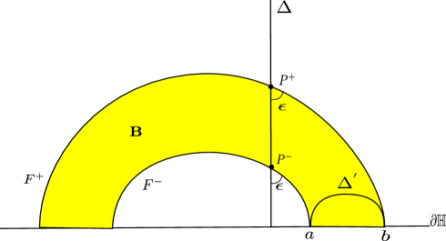
Figure 1. The band ${\bf B}$

Let ${\bf B}$ be the open band delimited by $F^{+}$ and $F^{-}$. When $P$ belongs to the interior of $P^{-}P^{+}$, the line $F(P)$ lies in the interior of the band ${\bf B}$ and $F(t)$ meets $\Delta^{\prime}$. It is clear from the definition of $F^{\pm}$ that

$$\lim_{P\to P_{-}}\,\omega(P)=0\,\,{\mathrm{a}nd}\lim_{P\to P_{+}}\,\omega(P)=\pi.$$

Hence by Assertion (1), $\omega$ is bijective.

∎

2.2 The $\epsilon$-edge

Let $\epsilon\in]0,\pi[$ and let $\Delta$, $\Delta^{\prime}$ be two lines with $d_{\mathbb{H}}(\Delta^{\prime},\Delta)>0$. Let $H$ be the the common perpendicular arc to $\Delta$ and $\Delta^{\prime}$ and let $S\in\Delta$ and $S^{\prime}\in\Delta^{\prime}$ be its endpoints.

By Lemma 3 there is a unique $P\in\Delta$ such that $\omega(P)=\epsilon$. The edge $e=P\Omega(P)$ will be called the $\epsilon$-edge of $\Delta$ and $\Delta^{\prime}$. For $\epsilon=\pi/2$, the $\epsilon$-edge is the perpendicular arc $H$.

Lemma 4.

Set $L=d_{\mathbb{H}}(P,P^{\prime})$ where $P^{\prime}=\Omega(P)$. If $\epsilon\neq\pi/2$, then

1. $H$ and $e$ intersect at their midpoints.

2. $d_{\mathbb{H}}(P,S)=d_{\mathbb{H}}(P^{\prime},S^{\prime})<L/2$.

Moreover the segment $SP$ is positively oriented whenever $\epsilon<\pi/2$.

Proof.

We have $\angle\Delta e=\epsilon$ and $\angle e\Delta^{\prime}=\overline{\epsilon}$. The sum of the four angles of the quadrilateral $Q:=SP\Omega(P)S^{\prime}$ is $2\pi$. It follows that a pair of opposite edges must intersect, so $e$ meets $H$ at some point $M$. The two triangles $SPM$ and $M\Omega(P)S^{\prime}$ have the same three angles, and are therefore isometric. In particular $d_{\mathbb{H}}(P,S)=d_{\mathbb{H}}(P^{\prime},S^{\prime})$.

It follows that $e$ and the arc $H=SS^{\prime}$ intersect at their midpoint $M$, thus we have $d_{\mathbb{H}}(P,M)=L/2$. Since $PM$ is the hypothenuse of the right-angled triangle $PSM$, we have $d_{\mathbb{H}}(P,S)<L/2$. The second claim follows. ∎

2.3 Hexagon trigonometry and edge colouring

Lemma 5.

Up to isometry, there exists a unique hyperbolic hexagon $H(\epsilon)$ whose sides all have the same length $L=L(\epsilon)$ and whose inner angles are alternately $\epsilon$ and $\overline{\epsilon}$.

Moreover we have

$$\cosh L=1+{1\over\sin\epsilon}.$$

Proof of the existence of $H(\epsilon)$ and of the formula for $\cosh L$.

Let $T$ be an oriented triangle whose angles are $\epsilon/2$, ${\overline{\epsilon}}/2$ and $\pi/3$ and let $X$ be the vertex at the $\pi/3$-angle. Let $\overline{T}$ be the triangle isometric to $T$ with opposite orientation. Let $H(\epsilon)$ be the hexagon obtained by alternately gluing three copies of $T$ and three copies of $\overline{T}$ around $X$. This hexagon satisfies the required conditions, so the existence is proved.

By the law of cosines for the triangle $T$, we have

$$\cosh L={\cos\epsilon/2\cos{\overline{\epsilon}}/2+\cos\pi/3\over\sin\epsilon/2\sin{\overline{\epsilon}}/2}$$

$$=1+{1\over 2\sin\epsilon/2\cos\epsilon/2}$$

$$=1+{1\over\sin\epsilon}.$$

Proof of the uniqueness.

Let $H$ be a hexagon whose sides all have the same length l, and whose angles are alternately $\epsilon$ and $\overline{\epsilon}$. Let $(A_{i})_{i\in\mathbb{Z}/6\mathbb{Z}}$ be the six vertices, arranged in a cyclic order. Moreover, we will assume that the angles at $A_{2}$, $A_{4}$ and $A_{6}$ are $\overline{\epsilon}$.

The triangles $A_{1}A_{2}A_{3}$, $A_{3}A_{4}A_{5}$ and $A_{5}A_{6}A_{1}$ have the same angles at the point $A_{2}$, $A_{4}$ and $A_{6}$, and the two sides originating from these points have the same length $l$. Hence they are isometric. It follows that the triangle $A_{1}A_{3}A_{5}$ is equilateral.

Let $X$ be the center of $A_{1}A_{3}A_{5}$, and let $T^{\prime}=A_{1}XA_{2}$ and ${\overline{T}}^{\prime}=A_{2}A_{3}X$. Since $T^{\prime}$ and ${\overline{T}}^{\prime}$ have same side lengths they are isometric, with opposite orientations. Hence $H$ is obtained by alternately gluing three copies of $T^{\prime}$ and three copies of $\overline{T}^{\prime}$ around $X$. It follows that the angles of $T^{\prime}$ are $\epsilon/2$, ${\overline{\epsilon}}/2$ and $\pi/3$. Therefore $T^{\prime}$ is isometric the the triangle $T$ of the existence proof. Hence $H$ is isometric to $H(\epsilon)$, proving uniqueness. ∎

We can alternately assign the colours blue and red to the sides of $H(\epsilon)$, as follows: If $S$, $S^{\prime}$ are consecutive sides with $\angle\mathrm{S\,S^{\prime}}=\epsilon$, then $S$ is red and $S^{\prime}$ is blue, or, quickly speaking, $\angle\mathrm{red\,blue}=\epsilon$. For $\epsilon\neq\pi/2$ this colouring is unique.

2.4 The Saccheri quadrilateral in $H(\pi/2)$

In the hexagon $H(\pi/2)$, let $S_{1},S_{2}$ and $S_{3}$ be three consecutive sides and let $D$ be the arc joining the vertex of $S_{1}{\smallsetminus}S_{2}$ and the vertex of $S_{3}{\smallsetminus}S_{2}$. Thus $S_{1}$, $S_{2}$, $S_{3}$ and $D$ are the four sides of a Saccheri quadrilateral. Set $L^{\prime}=l(D)$.

Lemma 6.

We have

$L^{\prime}<2L(\pi/2)$.

Proof.

Set $L=L(\pi/2)$. The perpendicular line at the middle of $S_{2}$ cuts the Saccheri quadrilateral into two isometric Lambert quadrilaterals. It follows that

$\sinh L^{\prime}/2=\cosh L/2\,\sinh L/2$,

or equivalently $\sinh^{2}L^{\prime}/2=4\sinh^{2}L/2$, which implies that $\cosh L^{\prime}=5$. On another hand $\cosh 2L=2\cosh^{2}2L-1=7$. It follows that $L^{\prime}<2L$. ∎

3. The three-holed sphere $\Sigma(k,\epsilon)$ and the pair of pants $\Pi(k,\epsilon)$

From now on, let $k\geq 3$ be an integer and let $\epsilon\in]0,\pi[$. We will often think of $\epsilon$ as being an acute angle, as in the figures of this section.

In this section, we will define a pair of pants $\Pi(k,\epsilon)$ endowed with a certain tesselation. We will first consider a three-holed sphere $\Sigma(k,\epsilon)$ which has two geodesic boundary components $C$ and $C^{\prime}$ and one piecewise geodesic boundary component $\mathcal{D}$. Since the inner angles of $\mathcal{D}$ are $<\pi$, it is homotopic to a unique geodesic $D$. Then $\Pi(k,\epsilon)$ is the pair of pants lying in $\Sigma(k,\epsilon)$, whose boundary components are $C,C^{\prime}$ and $D$.

3.1 The tesselated three-holed sphere $\Sigma(k,\epsilon)$

Let us start with the planar graph $\Gamma$ represented in Figure 2.

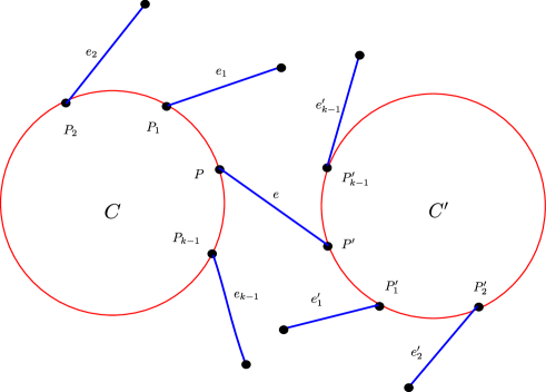
Figure 2. The graph $\Gamma$

It consists of two cycles $C$ and $C^{\prime}$ of length $k$, which are connected by an edge $e$ with endpoints $P\in C$ and $P^{\prime}\in C^{\prime}$. Starting from $P$ in an anticlockwise direction, the other points of $C$ are denoted by $P_{1},\dots,P_{k-1}$. For each $1\leq i\leq k-1$ there is an additional edge $e_{i}$, pointing outwards from $C$. One endpoint of $e_{i}$ is $P_{i}$ and the other endpoint has valency one. The vertices $P^{\prime}_{1},\dots,P^{\prime}_{k-1}$ of $C^{\prime}$ and the edges $e^{\prime}_{i}$ are defined similarly.

The edges of the cycles $C$ and $C^{\prime}$ are coloured in red, the other edges are coloured in blue. Now we will attach $2k-2$-hexagons $H(\epsilon)$ along the edges of $\Gamma$ to obtain a hyperbolic surface $\Sigma(\epsilon,k)$. It will be convenient to define a metric on $\Gamma$ by requiring that each edge, red or blue, has length $L=1+1/\sin\epsilon$.

First we attach two copies of $H(\epsilon)$ along five consecutive edges of $\Gamma$. The first copy, denoted $H_{1}(\epsilon)$, is glued along the edges $e_{k-1},\,P_{k-1}P,\,e,\,P^{\prime}P^{\prime}_{1}$ and $e^{\prime}_{1}$. The second copy, denoted $H_{2}(\epsilon)$, is glued along the edges $e^{\prime}_{k-1},\,P^{\prime}_{k-1}P^{\prime},\,e,\,PP_{1}$ and $e_{1}$, see Figure 3.

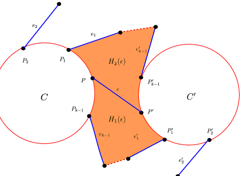
Figure 3. Gluing two the first two copies $H_{1}(\epsilon)$ and $H_{2}(\epsilon)$ to $\Gamma$

Next we attach the remaining $2k-4$ hexagons along three edges. Indeed, for each integer $i$ with $1\leq i\leq k-2$, we glue one copy of $H(\epsilon)$ along the edges $e_{i},\,P_{i}P_{i+1}$ and $e_{i+1}$ and, symmetrically, we glue another copy along $e_{i}^{\prime},\,P_{i}^{\prime\prime}P_{i+1}$ and $e_{i+1}^{\prime}$, see Figure 4.

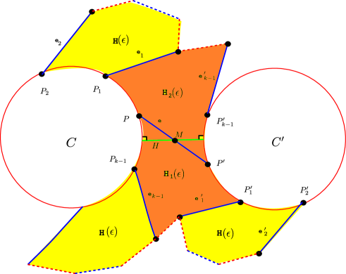
Figure 4. Gluing the remaining hexagons $H(\epsilon)$ to $\Gamma$

It is tacitly assumed that all gluings respect the metric and the colours of edges.

This defines a hyperbolic surface $\Sigma(k,\epsilon)$ which is homeomorphic to the 3-holed sphere $S_{0,3}$. Two boundary boundary components $C$ and $C^{\prime}$ of $\Sigma(k,\epsilon)$ are geodesics. The third component, call it $\mathcal{D}$, is piecewise geodesic.

Lemma 7.

The boundary component $\mathcal{D}$ is freely homotopic to a unique geodesic $D$. Moreover

1. $D$ lies in the interior of $\Sigma(k,\epsilon)$,

2. $D$ meets each arc $e_{i}$ and $e^{\prime}_{i}$ exactly once, and

3. $D$ does not intersect $e$.

Proof.

The curve $\mathcal{D}$ is piecewise geodesic. It is alternatively composed of $2(k-2)$ blue arcs and $2(k-2)$ red arcs. Since $k\geq 3$, $\mathcal{D}$ is not a geodesic. The inner angles of $\mathcal{D}$ are each less than $\pi$, therefore $\mathcal{D}$ is freely homotopic to a unique geodesic $D$ lying in the interior of $\Sigma(k,\epsilon)$.

Let $d$ be a blue edge. There is a 1-parameter family of curves $(\mathcal{D}_{t})_{t\in[0,1]}$, realizing a homotopy from $\mathcal{D}=\mathcal{D}_{0}$ to $D=\mathcal{D}_{1}$, such that the number of bigons formed by $d$ and $D=\mathcal{D}_{t}$ does not increase. Since there are no bigons formed by $d$ and $\mathcal{D}_{0}$, the geometric intersection numbers $i(d,\mathcal{D}_{t})$ is constant, which proves the last two claims. ∎

3.2 The pair of pants $\Pi(k,\epsilon)$ and its central octogon ${\bf Q}(\epsilon)$

The geodesic $D$ decomposes $\Sigma(k,\epsilon)$ into two pieces. The component $\Pi(k,\epsilon)\subset\Sigma(k,\epsilon)$ with geodesic curves $C$, $C^{\prime}$ and $D$ is a pair of pants.

The blue arcs decompose $\Pi(k,\epsilon)$ into two hexagons adjacent to the central edge $e$ and $2k-4$ quadrilaterals. Let ${\bf H}_{1}(\epsilon):=H_{1}(\epsilon)\cap\Pi(k,\epsilon)$ and ${\bf H}_{2}(\epsilon):=H_{2}(\epsilon)\cap\Pi(k,\epsilon)$ be the two hexagons of the decomposition. Their union ${\bf Q}(\epsilon):={\bf H}_{1}(\epsilon)\cup{\bf H}_{2}(\epsilon)$ is a convex octogon.

Let $H$ be the unique perpendicular arc joining $C$ and $C^{\prime}$ and let $S\in C$ and $S^{\prime}\in C^{\prime}$ be its endpoints. For $\epsilon=\pi/2$, we have $H=e$. Otherwise $H$ and $e$ meet as shown in the next lemma.

Lemma 8.

The arc $H$ lies in the octogon ${\bf Q}(\epsilon)$. When $\epsilon\neq\pi/2$, $H$ and $e$ intersect at their midpoint.

Moreover we have

1. $d(P,S)<L/2$, and

2. for $\epsilon<\pi/2$, the point $P$ belongs to ${\bf H}(\epsilon)$.

Proof.

The inner angles of ${\bf Q}(\epsilon)$ are less than $\pi$, hence there is an isometric embedding

$\pi:{\bf Q}(\epsilon)\to\mathbb{H}$.

Let $\Delta$ and $\Delta^{\prime}$ be the lines of $\mathbb{H}$ containing, respectively, the arcs $\pi\bigl{(}C\cap{\bf Q}(\epsilon)\bigr{)}$ and $\pi\bigl{(}C^{\prime}\cap{\bf Q}(\epsilon)\bigr{)}$. Let $\overline{H}$ be the common perpendicular arc to $\Delta$ and $\Delta^{\prime}$ and let $\overline{S}:=\overline{H}\cap\Delta$ and $\overline{S}^{\prime}:=\overline{H}\cap\Delta^{\prime}$ be its feet. By Lemma 4, we have

$d_{\mathbb{H}}(\pi(P),\overline{S})<L/2$.

Since $\pi\bigl{(}C\cap{\bf Q}(\epsilon)\bigr{)}$ is the geodesic arc of $\Delta$, centered at $\pi(P)$, of length $2L$, it follows that $\overline{S}$ is on the boundary of $\pi\bigl{(}C\cap{\bf Q}(\epsilon)\bigr{)}$. Similarly $\overline{S}^{\prime}$ is on the boundary of $\pi\bigl{(}C\cap{\bf Q}(\epsilon)\bigr{)}$. By convexity, the arc $\overline{H}$ lies in $\pi\bigl{(}{\bf Q}(\epsilon)\bigr{)}$.

Hence $H=\pi^{-1}(\overline{H})$ belongs to ${\bf Q}(\epsilon)$. The other claims follow from Lemma 4 and the fact that $\pi$ is an isometry. ∎

4. Trigonometry in the pair of pants $\Pi(k,\epsilon)$

Let $k\geq 3$ be an integer and let $\epsilon\in]0,\pi[$.

The pair of pants $\Pi(k,\epsilon)$ from the previous section is endowed with an $\epsilon$-edge $e$ joining $C$ and $C^{\prime}$, whose endpoints are $P\in C$ and $P^{\prime}\in C^{\prime}$. Recall that the length of $e$ is $L=\mathrm{arcosh}(1+1/\sin\,\epsilon)$. Let $H$ (resp. $h$, resp. $h^{\prime}$) be the unique common perpendicular arc to $C$ and $C^{\prime}$ (resp. to $C$ and $D$, resp. to $C^{\prime}$ and $D$). Cutting $\Pi(k,\epsilon)$ along $H\cup h\cup h^{\prime}$ provides the usual decomposition of the pair of pants into two right-angled hexagons.

4.1 Formula for $\cosh H$

As usual, we will use the same letter for an arc and for its length. As a matter of notation, let $S\in C$ and $S^{\prime}\in C^{\prime}$ be the endpoints of $H$.

Lemma 9.

We have

$$\cosh H=1+\sin\epsilon.$$

Proof.

When $\epsilon=\pi/2$, we have $e=H$ and $\cosh H=\cosh L=2$. Therefore we can assume that $\epsilon\neq\pi/2$.

By Lemma 8, $e$ and $H$ belong to the octogon ${\bf Q}(\epsilon)$ and intersect at their midpoint $M$. It follows that $SM=H/2$ and $PM=L/2$. By the sine law applied to the triangle $PSM$, we have

$$\sinh H/2=\sin\epsilon\sinh L/2.$$

From the identities $2\sinh^{2}H/2=\cosh H-1$ and $2\sinh^{2}L/2=\cosh L-1$, it follows that

$$\cosh H=1+\sin^{2}\epsilon\,(\cosh L-1).$$

By Lemma 5, we have $\cosh L-1=1/\sin\epsilon$, from which it follows that $\cosh H=1+\sin\epsilon$. ∎

4.2 Conventions concerning the asymptotics of angle functions

In what follows, we will consider analytic functions $f:]0,\pi[\to\mathbb{R}$. In order to study their asymptotic growth near $0$, we will use the following simplified notations. For any pair of functions $A,\,B:]0,\pi[\to\mathbb{R}$, the expression

$$A\sim B$$

means that

$$\lim_{\epsilon\to 0}{A\over B}=1.$$

Moreover the expression

$$A\sim*B$$

means that $A\sim aB$ for some positive real number $a$. Similarly, the expression $A<<B$ means that

$$\lim_{\epsilon\to 0}{A\over B}=0.$$

4.3 Length estimates

Lemma 10.

We have

$\cosh L\sim*\epsilon^{-1}$,

$H\sim*\epsilon^{1/2}$,

$d(S,P)=L/2+o(1)$.

Moreover, the lengths $h$ and $h^{\prime}$ are equal and we have

$h\sim*\epsilon^{k-1\over 2}$.

Proof.

Since by definition $\cosh L=1+1/\sin\epsilon$, we have $\cosh L\sim*\epsilon^{-1}$. By Lemma 9, we have $H\sim*\epsilon^{1/2}$ . By Lemma 8, $H$ and $e$ intersect at their midpoint $M$. Since

$|d(P,S)-d(P,M)|\leq d(S,M)=H$

we also have $|d(P,S)-L/2|\in o(1)$, which proves the third claim.

The perpendicular arcs $H,h$ and $h^{\prime}$ decompose the pair of pants $\Pi(k,\epsilon)$ into two isometric right-angled hexagons (see [5], Proposition 3.1.5) and let ${\bf A}$ be one of them.

Set $d=l(D)/2$. In an anticlockwise direction, the hexagon ${\bf A}$ has sides $h^{\prime},kL/2,H,kL/2,h$ and $d$. By the law of sines

$${\sinh kL/2\over\sinh h^{\prime}}={\sinh kL/2\over\sinh h}$$

and therefore $h=h^{\prime}$.

In order to prove the final statement, we first estimate $\cosh d$. By the law of cosines, we have

$$\cosh H={\cosh^{2}kL/2+\cosh d\over\sinh^{2}kL/2}$$

$$=1+{1+\cosh d\over\sinh^{2}kL/2}.$$

It follows that

$$1+\cosh d=\sinh^{2}kL/2(\cosh H-1),$$

and $\cosh d\sim*e^{kL}H^{2}\sim*\epsilon^{1-k}$. By the law of sines, we have

$$\sinh h={\sinh H\sinh kL/2\over\sinh d}$$

and therefore $h\sim\sinh h\sim*\epsilon^{(k-1)/2}$. ∎

4.4 The angles $\omega_{i}$ and $\omega_{i}^{\prime}$

By Lemma 7, the geodesic $D$ meets the arcs $e_{i}$ and $e_{i}^{\prime}$ exactly once each, so we can define

$\omega_{i}:=\angle De_{i}$ and $\omega^{\prime}_{i}:=\angle De^{\prime}_{i}$.

Lemma 11.

We have

1. $\omega_{i}=\omega^{\prime}_{i}$, for any $1\leq i\leq k-1$.

2. $\omega_{1}<\omega_{2}<\dots<\omega_{k-1}$.

Proof.

By definition of $\Sigma(k,\epsilon)$ and $\Pi(k,\epsilon)$, there is a isometric rotation of angle $\pi$ around the midpoint $M$ of the arc $PP^{\prime}$. It follows that $\omega_{i}=\omega^{\prime}_{i}$ for any $i$.

The pair of arcs $e_{1}$ and $e_{k-1}$ decompose $\Pi(k,\epsilon)$ into two connected components. Let ${\bf Q}_{0}$ be the contractible component, which is a quadrilateral whose sides are $e_{1}$, $e_{k-1}$, an arc of $C$ and an arc of $D$. It is larger than the quadrilateral ${\bf Q}$ of Figure 5, because the top edge is $e_{1}$ instead of $h$.

Let $\pi:{\bf Q}_{0}\to\mathbb{H}$ be a isometric embedding. Set $\Delta^{\prime}=\pi(D\cap{\bf Q})$ and let $\Delta$ be the line of $\mathbb{H}$ containing the arc $\pi(C\cap{\bf Q}_{0})$. The arcs $\pi(e_{1}),\dots,\pi(e_{k-1})$ belongs to the $\epsilon$-pencil $\mathcal{F}_{\epsilon}(\Delta)$ of the line $\Delta$. The second claim therefore follows from Lemma 3 (1). ∎

4.5 Angle estimates

Lemma 12.

For any $i=1,2,\dots,k-1$, we have

$$\lim_{\epsilon\to 0}\omega_{i}=\lim_{\epsilon\to 0}\omega^{\prime}_{i}=0.$$

Proof.

By Lemma 11, it is enough to show that $\lim_{\epsilon\to 0}\omega_{k-1}=0$.

The pair of arcs $h$ and $e_{k-1}$ cut $\Pi(k,\epsilon)$ into two connected components, where ${\bf Q}$ is the contractible component, as shown in Figure 5. Then ${\bf Q}$ is a convex quadrilateral whose vertices are the endpoints of $h$, namely $N:=h\cap C$ and $\Omega:=h\cap D$ and the endpoints of $e_{k-1}$, namely $\Omega_{k-1}:=e_{k-1}\cap D$ and $P_{k-1}$.

Let $v$ be the diagonal of ${\bf Q}$ joining $P_{k-1}$ and $\Omega$. Set

$\epsilon^{-}=\angle Cv$, $\epsilon^{+}=\angle ve_{k-1}$, $\gamma^{-}=\angle hv$ and $\gamma^{+}=\angle vD$. By definition we have

$\epsilon^{-}+\epsilon^{+}=\epsilon$, and $\gamma^{-}+\gamma^{+}=\pi/2$.

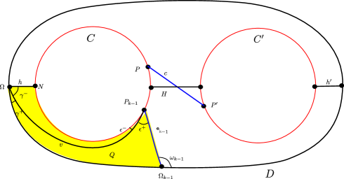
Figure 5. This figure illustrates the notation from the proofs of Lemmas 12 and 11.

First, we look at the trigonometry of the triangle $P_{k-1}N\Omega$. Set $a=d(N,P_{k-1})$. We have $a=(k/2-1)L+d(S,P)$. By Lemma 9, we have $d(S,P)=L/2+o(1)$, therefore $a=uL+o(1)$, where $u=(k-1)/2$. It follows that

$$\cosh a\sim*\epsilon^{-u}.$$

Since $\cosh v=\cosh a\cosh h$, it follows from Lemma 10 that

$$\cosh v\sim\cosh a\sim*\epsilon^{-u}.$$

By the sine law, we have $\sin\epsilon^{-}=\sinh h/\sinh v$. It follows from Lemma 10 and the previous estimate that $\epsilon^{-}\sim*\epsilon^{2u}$. Since $k\geq 3$, we have $\epsilon^{-}<<\epsilon$ and therefore

$$\epsilon^{+}\sim\epsilon.$$

By combining the cosine and sine laws, we have $\cos\gamma^{-}=\sin\epsilon^{-}\cosh a=\sinh h\cosh a/\sinh v$, and therefore

$$\cos\gamma^{-}\sim*\epsilon^{u}.$$

Next, we will look at the trigonometry of the triangle $P_{k-1}\Omega\Omega_{k-1}$. Since $\sin\gamma^{+}=\cos\gamma^{-}$, we have

$$\gamma^{+}\sim\sin\gamma^{+}\sim*\epsilon^{u}.$$

Using the cosine law, we have $\cos{\overline{\omega}_{k-1}}=\sin\epsilon^{+}\sin\gamma^{+}\cosh v-\cos\epsilon^{+}\cos\gamma^{+})$. Adding one on each side and using that $\cos{\overline{\omega}_{k-1}}=-\cos\omega_{k-1}$, we obtain

$$1-\cos\omega_{k-1}=\sin\epsilon^{+}\sin\gamma^{+}\cosh v+(1-\cos\epsilon^{+}\cos\gamma^{+}).$$

We will now estimate the right term of the previous identity. Using a Taylor expansion, it is clear that

$$1-\cos\epsilon^{+}\cos\gamma^{+}\in O(\epsilon^{2})+O(\epsilon^{2u})=O(\epsilon^{2}).$$

On the other hand, we have

$$\sin\epsilon^{+}\sin\gamma^{+}\cosh v\sim*\epsilon.$$

Hence we have $1-\cos\omega_{k-1}\sim*\epsilon$, i.e.

$$\omega_{k-1}\sim*\epsilon^{1/2},$$

and therefore we have proved that $\lim_{\epsilon\to 0}\omega_{k-1}=0$.

∎

5. Sanki’s paths and curve duality

For the whole section, we assume given an oriented topological closed manifold $\mathcal{S}$ of genus $g$ endowed with an isomorphism $\rho:\Pi_{g}\to\pi_{1}({\mathcal{S}})$, defined modulo the inner conjugations. It will be called the marking of the topological surface $\mathcal{S}$.

We will consider a set $\mathrm{Tess}(\mathcal{S})$ of hexagonal tesselations of $\mathcal{S}$, which are defined by a set $\mathcal{C}_{R}$ of red curves and a set $\mathcal{C}_{B}$ of blue curves. Following an idea of [15][2], we define, for each $\tau\in\mathrm{Tess}(\mathcal{S})$, a path, called a Sanki’s path, $\sigma:]0,2\pi[\rightarrow\mathcal{T}_{g}$. Intuitively, Sanki’s path are infinitesimal analogs of Penner’s construction [13] of quasi-Anosov homeomorphisms.

When $\tau$ satisfies some additional properties, we define, for each blue curve $B$ a dual object $B^{*}$, which is a linear combination of three curves with coefficients $\pm 1/2$. Of course, $B^{*}$ is not a multicurve, but its length function $L(B^{*})$ is well defined. The first result of the paper is Theorem 15, showing a kind of duality between $B$ and $B^{*}$. It is expressed in terms of the Poisson bracket $\{L(A),L(B^{*})\}$ relative to the Weil-Petersson symplectic form [19].

5.1 The set of hexagonal tesselations $\mathrm{Tess}(\mathcal{S})$

Let $\mathcal{H}$ be an oriented topological hexagon whose six sides are alternatively coloured in red and blue. Strictly speaking $\mathcal{H}$ is a closed disc whose boundary is divided into six components, but the terminology hexagon is more suggestive.

Let $\mathrm{Tess}(\mathcal{S})$ be the set of all tesselations $\tau$ of $\mathcal{S}$ satisfying the following two axioms:

(AX1) The tiles are homeomorphic to $\mathcal{H}$ and they are glued pairwise along edges of the same colour.

(AX2) Each vertex of the tesselation has valence four.

The last axiom implies that each vertex is the endpoint of four edges, which are alternately red and blue. The graph consisting of red edges is a disjoint union of cycles. Those cycles are called the red curves of the tesselation and the set of red curves is denoted $\mathcal{C}_{red}$. Similarly, we define the blue curves of the tesselation and the set $\mathcal{C}_{blue}$ of blue curves. The set $\mathrm{Curv}(\tau):=\mathcal{C}_{red}\cup\mathcal{C}_{blue}$ is called the set of curves of the tesselation.

5.2 Sanki paths

We will now define the Sanki’s path of a tessalation $\tau\in\mathrm{Tess}(\mathcal{S})$. Let $\epsilon\in]0,\pi[$. Define a metric on the $1$-skeleton $\tau_{1}$ of $\tau$ by requiring that all edges have length $L$. Recall that $L=\mathrm{arcosh}(1+1/\sin\epsilon)$ is the side lengths of the hexagon $H(\epsilon)$ defined in Subsection 2.3.

For each closed face $f$ of the tesselation, let $\phi_{f}:H(\epsilon)\to f$ be a homeomorphism such that its restriction to the boundary $\delta f:\partial H(\epsilon)\to\partial f$ preserves the metric and the colour of the edges.

A tesselation of $\mathcal{S}$ is obtained where each tile is endowed with a hyperbolic structure. Along each edge of $\tau_{1}$, two geodesic arcs have been glued isometrically. Around each vertex of $\tau_{1}$, the four angles are alternatively $\epsilon$ and $\overline{\epsilon}$, hence their sum is $2\pi$. By Theorem 1.3.5 of [5], there is a hyperbolic metric on $\mathcal{S}$ extending the metric of the tiles. Together with the marking $\rho$ of ${\mathcal{S}}$, we obtain a well defined marked hyperbolic surface $S_{\tau}(\epsilon)$.

The idea of deforming right-angled regular polygons by polygons with angles of value alternatively $\epsilon$ and $\pi-\epsilon$ first appeared in [15] and it was used in [2]. Therefore the corresponding path $\sigma_{\tau}:]0,\pi[\rightarrow\mathcal{T}_{g}$, $\epsilon\mapsto S_{\tau}(\epsilon)$ will be called the Sanki’s path of the tessalation $\tau$. Since the function $\cosh L=1+1/\sin\epsilon$ is analytic, the path $\sigma_{\tau}$ is analytic.

It should be noted that, around each vertex the colours, blue or red, and the angles, $\epsilon$ or $\overline{\epsilon}$, of the edges alternate. Therefore the blue curves and the red curves are geodesics with respect to the hyperbolic metric on $S_{\tau}(\epsilon)$.

5.3 $k$-regular tesselations

For a closed oriented surface $\mathcal{S}$, $(AX1)$ and $(AX2)$ is the minimal set of axioms required to define the Sanki’s path. We will now define more axioms. The axiom (AX3) will ensure that the curves have the same length, while the axioms (AX4) and (AX5) are connected with the duality construction.

Let $k\geq 2$ be an integer and let $\mathcal{S}$ be a closed surface. A tesselation $\tau\in{\mathrm{Tess}}(\mathcal{S})$ is called a $k$-regular tesselation iff it satisfies the following axiom

(AX3) Each curve of $\tau$, blue or red, consists of exactly $k$ edges.

Denote by Tess$(\mathcal{S},k)$ the set of all $k$-regular tesselations. For any $k$-regular tesselation $\tau$, we will consider two additional axioms. The first axiom is

(AX4) A blue edge and a red curve meet at most once.

Assume now that $\tau\in\mathrm{Tess}(\mathcal{S},k)$ satisfies (AX4). Let $R$ be a red curve, let $b,b^{\prime}$ be two blue edges adjacent to $R$ and let $N$ be a small regular neigborhood of $R$. Since $\mathcal{S}$ is oriented, $N{\smallsetminus}R$ consists of two open annuli, $N^{\pm}$. By axiom (AX4), $b$ has only one endpoint in $R$, therefore $b$ intersect either $N^{+}$ or $N^{-}$. Similarly, $b^{\prime}$ intersect either $N^{+}$ or $N^{-}$. We say that $b,b^{\prime}$ are adjacent on the same side of $C$ if they both intersect $N^{+}$ or if they both intersect $N^{-}$. Our last axiom is

(AX5) Two distinct blue edges are adjacent on the same side of at most one red curve.

Denote by $\mathrm{Tess}_{45}(\mathcal{S},k)$ the set of $k$-regular tesselations satisfying the axioms (AX4) and (AX5).

4.4 The isometric embedding $\pi_{b}:\Pi(k,\epsilon)\to S_{\tau}(\epsilon)$

From now on, assume that $k\geq 3$. Let $\tau\in\mathrm{Tess}_{45}(\mathcal{S},k)$. In order to define the duality, we first associate to each blue edge a pair of pants $\Pi(k,\epsilon)\subset S_{\tau}(\epsilon)$.

Let $b$ be a blue edge with endpoints $Q$ and $Q^{\prime}$, and let $R$ and $R^{\prime}$ be the red curves passing through $Q$ and $Q^{\prime}$. By axiom (AX4), the two curves $R$ and $R^{\prime}$ are distinct, so the graph $\Gamma_{0}:=R\cup R^{\prime}\cup b$ is a union of two circles connected by an edge. Since $\mathcal{S}$ is oriented, a small normal open neighbourhood $N$ of $\Gamma_{0}$ is a thickened eight. Then $R\cup R^{\prime}$ cuts $N$ into three components, two of them are homeomorphic to annuli and the third one, call it $\Omega$, contains $b$.

In a planar representation of $\Gamma_{0}$, $\Omega$ is the exterior of $R\cup R^{\prime}$. Since $R$ and $R^{\prime}$ are boundary components of $\Omega$, these curves inherit an orientation. By axiom (AX3), $R$ contains $k$ vertices of the tesselation. Starting from $Q$ in the anticlockwise direction, the other $k-1$ points of $R$ are denoted by $Q_{1},\dots,Q_{k-1}$. For each $1\leq i\leq k-1$ let $b_{i}$ be the blue edge starting at $Q_{i}$ on the same side as $b$. The points $Q^{\prime}_{1},\dots,Q^{\prime}_{k-1}$ of $R^{\prime}$ and the edges $b^{\prime}_{i}$ are defined similarly. Adding the edges $b_{i},b^{\prime}_{i}$ to the graph $\Gamma_{0}$, we obtain a graph $\overline{\Gamma}$.

Let $\epsilon\in]0,\pi[$ and recall that $S_{\tau}(\epsilon)$ is the tesselated surface $S_{g}$ representing a point in $\mathcal{T}_{g}$.

Let $\Gamma$ be the graph defined in Section 4.1. There is a local isometry $\pi:\Gamma\to\overline{\Gamma}$ such that $\pi(P)=Q$, $\pi(P_{i})=Q_{i}$, $\pi(e_{i})=b_{i}$, $\pi(C)=R$, $\pi(P^{\prime})=Q^{\prime}$, $\pi(P^{\prime}_{i})=Q^{\prime}_{i}$, $\pi(e_{i})=b_{i}$ and $\pi(C^{\prime})=R^{\prime}$. Clearly, it can be extended uniquely to a local isometry $\pi:\Pi(k,\epsilon)\to S_{\tau}(\epsilon)$. Let $\pi_{b}$ be its restriction to $\Pi(k,\epsilon)$.

Lemma 13.

The map $\pi_{b}:\Pi(k,\epsilon)\to S_{\tau}(\epsilon)$ is an isometric embedding.

Proof.

Since $b$ joins $R$ and $R^{\prime}$, it follows from Axiom (Ax4) that $R$ and $R^{\prime}$ are distinct. By Axioms (Ax4) and (Ax5), the point $Q_{i}$, respectively $Q^{\prime}_{j}$ is the unique endpoint of $b_{i}\cap\Omega$, respectively of $b^{\prime}_{j}\cap\Omega$. Hence the blue edges $b$, $b_{i}$ and $b^{\prime}_{j}$ are all distinct. For any two edges $e\neq e^{\prime}$ of $\Gamma\cap\Pi(k,\epsilon)$, we therefore have $\pi(e)\neq\pi(e^{\prime})$.

Let $F,F^{\prime}$ be two faces of $\Pi(k,\epsilon)$ such that $\pi(F)=\pi(F^{\prime})$. Since each face $F$ or $F^{\prime}$ has at least two blue edges in $\Gamma$, it follows that $F$ and $F^{\prime}$ contain a common blue edge $e\subset\Gamma$. It follows easily that $F=F^{\prime}$.

Consequently, the restriction of $\pi$ to $\Pi(k,\epsilon){\smallsetminus}\mathcal{D}$ is injective. By Lemma 7, $\Pi(k,\epsilon)$ lies in $\Sigma(k,\epsilon){\smallsetminus}\mathcal{D}$. Therefore $\pi$ induces an isometric embedding $\pi_{b}:\Pi(k,\epsilon)\to S_{\tau}(\epsilon)$. ∎

5.5 The dual functions $L(B^{*})$

Let $\tau\in\mathrm{Tess}_{45}(\mathcal{S},k)$ for some integer $k\geq 3$.

We are now going to define the dual function $L(B^{*})$, for any blue curve of $B$ of the tesselation. Choose anf fix one edge $b$ of $B$. Let $R$, $R^{\prime}$ be the two red curves containing the endpoints of $b$ and set $D_{b}=\pi_{b}(D)$. Set

$$L(B^{*})={1\over 2}(L(R)+L(R^{\prime})-L(D_{b})).$$

Informally speaking, $L(B^{*})$ is the length function associated with the “dual curve” $B^{*}=1/2(R+R^{\prime}-D_{b})$. Strictly speaking, the function $L(B^{*})$ depends of the choice of the edge $b$.

For any $F,G\in C^{\infty}(\mathcal{T}_{g})$, let $\{F,G\}$ be their Poisson bracket induced by the the Weil-Petersson symplectic form on $\mathcal{T}_{g}$, see e.g. [19]. The duality between $B$ and $B^{*}$ is demonstrated in the next lemma.

Lemma 14.

Let $\tau\in\mathrm{Tess}_{45}(\mathcal{S},k)$ and let $\sigma_{\tau}:]0,\pi[\rightarrow\mathcal{T}_{g}$ be the associated Sanki path.

For any $A,\,B\in\mathcal{C}_{blue}$, we have

$$\lim_{\epsilon\to 0}\{L(A),L(B^{*})\}(\sigma_{\tau}(\epsilon))=\delta_{A,B},$$

where $\delta_{A,B}$ is the Kronecker delta.

Proof.

Let $B\in\mathcal{C}_{blue}$. By definition there is an edge $b$ of $B$ such that $2L(B^{*})=L(R)+L(R^{\prime})-L(D_{b})$ where $R$ and $R^{\prime}$ are the two red curves containing the endpoints of $b$.

Set $\overline{\Pi}=\pi_{b}({\Pi}(k,\epsilon))$ and $\overline{D}=\pi_{b}(D_{b})$. For each $i\in\{1,2,\dots,k-1\}$, set

$\beta_{i}=c_{i}\cap\overline{\Pi}(k,\epsilon)$ and $\beta_{i}^{\prime}=c_{i}^{\prime}\cap\overline{\Pi}(k,\epsilon)$.

By Lemma 13, $\beta_{i}$ is an arc, with one endpoint $P_{i}$ in $R$ and the other endpoint $\Omega_{i}$ on $\overline{D}$. Similarly, $\beta_{i}^{\prime}$ is an arc, with one endpoint $Q_{i}^{\prime}$ in $R^{\prime}$ and the other endpoint, say $\Omega_{i}^{\prime}$, belongs to $\overline{D}$. We have

1. $\beta_{i}$ does not intersect $R^{\prime}$,

2. $\beta_{i}\cap R=Q_{i}$ and $\angle R\beta_{i}=\epsilon$

3. $\beta_{i}\cap\overline{D}=\Omega_{i}$ $\angle\overline{D}\beta_{i}=\omega_{i}$,

where the angles $\omega_{i}$ are defined in Section 4.4. Similarly, we have

1. $\beta_{i}^{\prime}$ does not intersect $R$,

2. $\beta_{i}^{\prime}\cap R^{\prime}=P_{i}^{\prime}$ and $\angle R\beta_{i}=\epsilon$

3. $\beta_{i}^{\prime}\cap\overline{D}=\Omega_{i}$ $\angle\overline{D}\beta_{i}^{\prime}=\omega_{i}^{\prime}$.

Let $A\in\mathcal{C}_{blue}$ be another blue curve. Set

$I=\{i\mid 1\leq i\leq k-1\,\mathrm{and}\,\beta_{i}\subset A\}$, and

$I^{\prime}=\{i\mid 1\leq i\leq k-1\,\,\mathrm{and}\beta_{i}^{\prime}\subset A\}$.

When $A\neq B$, the curve $A$ meets $R\cup R^{\prime}\cup D_{b}$ exactly at the points $P_{i},\Omega_{i}$ for $i\in I$ and $P_{i}^{\prime},\Omega_{i}^{\prime}$ for $i\in I$. Therefore by Wolpert’s formula [18], we have

$\{L(A),L(R)+L(R^{\prime})-L(D_{b})\}(\sigma_{\tau}(\epsilon))$

$=[\sum_{i\in I}\cos\epsilon-\cos\omega_{i}]+[\sum_{i\in I^{\prime}}\cos\epsilon-\cos\omega_{i}^{\prime}]$.

By Lemma 12, we have

$$\lim_{\epsilon\to 0}\omega_{i}=0,$$

and therefore

$$\lim_{\epsilon\to 0}\{L(A),L(B^{*})\}(\sigma_{\tau}(\epsilon))=0$$

When $A=B$, the computation is similar except that, in addition to the arcs $\beta_{i}$ for $i\in I$ and $\beta^{\prime}_{i}$ for $i\in I^{\prime}$, the geodesic $A$ contains $b$. Therefore, one obtains

$\{L(A),L(R)+L(R^{\prime})-L(D_{b})\}(\sigma_{\tau}(\epsilon))$

$=2\cos\epsilon+[\sum_{i\in I}\cos\epsilon-\cos\omega_{i}]+[\sum_{i\in I}\cos\epsilon-\cos\omega_{i}^{\prime}]$,

and therefore

$$\lim_{\epsilon\to 0}\{L(A),L(A^{*})\}(\sigma_{\tau}(\epsilon))=1.$$

∎

5.6 The duality theorem

Suppose $k\geq 3$ and choose $\tau\in\mathrm{Tess}(\mathcal{S},k)$. Recall that $\sigma_{\tau}:]0,\pi[\to\mathcal{T}_{g}$ is the Sanki path.

Theorem 15.

Assume that $\tau$ satisfies the axioms (AX4) and AX(5). Then for any $\epsilon\in]0,\pi[$ outside some finite set $F$, the set

$$\{\mathrm{d}L(C)\mid C\in\mathrm{Curv}(\tau)\}$$

is linearly independent at the point $\sigma_{\tau}(\epsilon)$.

Proof.

For $\epsilon\in]0,\pi[$, let $\delta(\epsilon)$ be the determinant of the square matrix

$$(\{L(A),L(B^{*})\}(\sigma_{\tau}(\epsilon)))_{A,B\in\mathcal{C}_{blue}},$$

and set $F=\{\epsilon\in]0,\pi[\,\mid\delta(\epsilon)=0\}$.

By Lemma 14, we have $\lim_{\epsilon\to 0}\,\delta(\epsilon)=1$. Moreover, changing the orientation of $\mathcal{S}$ amounts to replacing $\epsilon$ by $\overline{\epsilon}$, so we also have $\lim_{\epsilon\to\pi}\,\delta(\epsilon)=\pm 1$. Since $\delta$ is an analytic function on $]0,\pi[$, it follows that $F$ is finite.

It remains to show that, for $\epsilon\notin F$, the differentials at $\sigma_{\tau}(\epsilon)$ of the set of length functions $\{L(C)\mid C\in\mathrm{Curv}(\tau)\}$ are linearly independent.

Let $\epsilon\notin F$. Let $(a_{A})_{A\in\mathrm{Curv}(\tau)}$ be an element of $\mathbb{R}^{|\mathrm{Curv}(\tau)|}$ such that

$$\sum_{A\in\mathrm{Curv}(\tau)}\,a_{A}dL(A)|_{\sigma_{\tau}(\epsilon)}=0.$$

Let $B\in\mathcal{C}_{blue}$. Recall that $B^{*}$ is a linear combination of two red curves $R,R^{\prime}$ and a certain geodesic $D_{b}$. Neither the geodesics $D_{b}$ nor the red curves meet any red curve transversally. Hence we have $\{L(C),L(B^{*})\}=0$ for any red curve $C$. It follows that

$$\sum_{A\in\mathcal{C}_{blue}}\{a_{A}L(A),L(B^{*})\}$$

is zero at $\sigma_{\tau}(\epsilon)$. Since $\delta(\epsilon)\neq 0$, we have $a_{A}=0$ for any $A\in\mathcal{C}_{blue}$.

Therefore, it follows that

$$\sum_{A\in\mathcal{C}_{red}}\,a_{A}dL(A)|_{\sigma_{\tau}(\epsilon)}=0.$$

Since it is a subset of some Fenchel-Nielsen coordinates, the set of differentials $\{\mathrm{d}L(A)\mid A\in\mathcal{C}_{red}\}$ is linearly independent. Therefore we also have $a_{A}=0$ for any $A\in\mathcal{C}_{red}$.

Hence the differentials $(\mathrm{d}L(A))_{A\in\mathrm{Curv}(\tau)}$ are linearly independent at $\sigma_{\tau}(\epsilon)$. ∎

6. Local structure of ${\mathcal{P}}_{g}$ along a Sanki’s path

Our previous work [10] provides a systematic construction of $k$-regular tesselations $\tau$. To apply Theorem 15, we first show that the axioms $(AX4)$ and $(AX5)$ are automatically satisfied when the curves of $S_{\tau}(\pi/2)$ are the systoles.

Then we deduce the local structure of the Thurston’s spine along a Sanki’s path.

To prove the main result, we will apply Theorem 15 to the tesselations $\tau_{g}$ of the surface $S_{g}$ obtained in [10]. Obviously they satisfy the axioms $(AX1-3)$ and it remains to prove that the tesselations $\tau_{g}$ also satisfy $(AX4)$ and $(AX5)$.

6.1 Verification of the axioms $(AX4)$ and $(AX5)$

As usual, suppose $\mathcal{S}$ is a surface of genus $g\geq 2$, $k\geq 3$ and $\tau\in{\mathrm{Tess}}(\mathcal{S},k)$.

Lemma 16.

Assume that the set of systoles of $S_{\tau}(\pi/2)$ is the set of curves of $\tau$. Then the tesselation $\tau$ satisfies the axioms (AX4) and (AX5).

Proof.

By a well-known lemma of riemannian geometry, two distinct systoles intersect in at most one point, therefore (AX4) is satisfied.

The proof of Axiom (AX5) is more delicate. Let $C,C^{\prime}\in\mathcal{C}$ and let $c,d$ be two distinct blue edges connecting $C$ and $C^{\prime}$ on the same side. Let $(P,P^{\prime})\in C\times C^{\prime}$ be the endpoints of $c$, and let $(Q,Q^{\prime})\in C\times C^{\prime}$ be the endpoints of $d$, as shown in Figure 6.

Since $c$ and $d$ are adjacent to $C$ on the same side, there is a planar representation of $C$ and $C^{\prime}$ where $c$ and $d$ are on the exterior of $C$. This planar representation provides an orientation of $C$ and $C^{\prime}$, called the direct orientation.

Let $F_{1}$ and $F_{2}$ be the two hexagons containing $d$. Set $f_{1}=F_{1}\cap C$, $f_{2}=F_{1}\cap C$, $f_{1}^{\prime}=F_{1}\cap C$, $f_{2}^{\prime}=F_{1}\cap C$. By definition, $f^{\prime}_{1},d$ and $f_{1}$ are consecutive edges of $F_{1}$. We can assume $f^{\prime}_{1},d$ and $f_{1}$ are ordered relative to the direct orientation. Consequently $f_{2}$ follows $f_{1}$ relative to the orientation of $C$. Since $\mathcal{S}$ is oriented, $f^{\prime}_{1}$ follows $f^{\prime}_{2}$ in the direct orientation of $C^{\prime}$. Therefore the relative position of $F_{1}$ and $F_{2}$ along $C$ and $C^{\prime}$ is as in Figure 6.

Figure 6. Respective positions of $F_{1}$ and $F_{2}$. They appear on the left side and the right sides of the figure: it should be understood that they lie on a cylinder.

For $i=1$ or $2$, let $\gamma_{i}$ be the arc of $C$ from $Q$ to $P$ and containing $f_{i}$. Similarly let $\gamma_{i}^{\prime}$ be the arc of $C^{\prime}$ from $P^{\prime}$ to $Q$ and containing $f_{i}^{\prime}$. Let us orient $c$ from $P$ to $P^{\prime}$ and $d$ from $Q^{\prime}$ to $Q$.

The arc $\gamma_{1}$, $\gamma_{2}$, $\gamma_{1}^{\prime}$ and $\gamma_{2}^{\prime}$ cover $C\cup C^{\prime}$, therefore we have

$L(\gamma_{1})+L(\gamma_{1}^{\prime})+L(\gamma_{2})+L(\gamma_{2}^{\prime})=2kL$.

It is possible to assume without loss of generality that

$L(\gamma_{1})+L(\gamma_{1}^{\prime})\leq kL$.

The path $\gamma_{1}$ consists of $L(\gamma_{1})/L$ edges. Let $g_{1}$ be the last edge of $\gamma_{1}$. Similarly, let $g_{1}^{\prime}$ be the first edge of $\gamma_{1}^{\prime}$. By definition, $g_{1}$ contains $P$ and $g_{1}^{\prime}$ contains $P^{\prime}$. Let $G_{1}$ be the hexagon with the three consecutive edges $g_{1}$, $c$ and $g_{1}^{\prime}$.

Now $f_{1}\neq g_{1}$ and $f_{1}^{\prime}\neq g_{1}^{\prime}$, otherwise the edge $d$ would join $g_{1}$ and $g^{\prime}_{1}$. Hence we have $F_{1}\neq G_{1}$. Therefore there is a factorization $\gamma_{1}=f_{1}*\delta_{1}*g_{1}$, where $\delta_{1}$ is the geodesic arc between $f_{1}$ and $g_{1}$ and where the notation $*$ stands for the concatenation of paths. Similarly, there is a factorization $\gamma_{1}^{\prime}=f_{1}*\delta_{1}^{\prime}*g_{1}$.

We show now that the loop

$\gamma:=\gamma_{1}*c*\gamma_{1}^{\prime}*d$,

is not null-homotopic. Assume otherwise. Set $S_{g}=S_{\tau}(\pi/2)$, let $\pi:\mathbb{H}\to S_{g}$ be the universal cover of $S_{g}$ and let $\tilde{\gamma}$ be a lift of $\gamma$ in $\mathbb{H}$. Since $\gamma$ is composed of four geodesic arcs, and the angles between them are $\pi/2$, the lift $\tilde{\gamma}$ would bound a quadrilateral whose inner angles are all $\pi/2$ or $3\pi/2$ which is impossible. It follows that $\gamma$ is not null-homotopic.

The hexagon $F_{1}$ contains a Saccheri quadrilateral whose basis is $d$ and with feet given by $f_{1}$ and $f^{\prime}_{1}$. Let $d^{\prime}$ be the fourth side, oriented from $f^{\prime}_{1}$ to $f_{1}$. As a path, $d^{\prime}$ is homotopic to $f^{\prime}_{1}*d*f_{1}$.

Similarly, let $c^{\prime}$ be the last side, oriented from $g_{1}$ to $g^{\prime}_{1}$, of the Saccheri quadrilateral in $G_{1}$ whose basis is $c$ and whose feet are $g_{1}$ and $g^{\prime}_{1}$. Similarly, $c^{\prime}$ is homotopic to $g_{1}*d*g^{\prime}_{1}$.

Up to a reparametrization, we have

$\gamma=\delta_{1}*g_{1}*c*g^{\prime}_{1}*\delta_{1}^{\prime}*f_{1}^{\prime}*d*f_{1}$.

Hence $\gamma$ is homotopic to $\tilde{\gamma}=\delta_{1}*c^{\prime}*\delta_{1}^{\prime}*d^{\prime}$. Since we have $L(c^{\prime})=L(d^{\prime})=L^{\prime}$, we have

$L(\tilde{\gamma})=L(\gamma_{1})+L(\gamma_{1}^{\prime})+2L^{\prime}-4L<kL$

by Lemma 6, which contradicts that $\mathcal{C}$ is the set of systoles. ∎

6.2 Two corollaries

We will now derive two corollaries concerning the structure of ${\mathcal{P}}_{g}$ at the neighborhood of a Sanki’s path.

Given a finite set of curves ${\mathcal{C}}=\{C_{1},C_{2},\dots,C_{n}\}$, let $E({\mathcal{C}})$ be the set of $x\in{\mathcal{T}}_{g}$ such that

$L(C_{1})(x)=L(C_{2})(x)=\dots=L(C_{n})(x)$.

Also let ${\mathrm{Sys}}\,({\mathcal{C}})$ be the set of points $x\in{\mathcal{P}}_{g}$ such that ${\mathcal{C}}$ is the set of systoles at $x$.

Let $X\subset{\mathcal{P}}_{g}$ be a locally closed subset, and let $x\in\overline{X}$. We say that $X$ is locally a smooth manifold at $x$ if $U\cap X$ is a smooth manifold for some open neighborhod of $X$. When it is the case, the local codimension $\mathrm{codim}_{x}\,X$ is well defined. Our previous definition do not require that $x$ belongs to $X$.

Corollary 17.

Let $\tau\in{\mathrm{Tess}}(\mathcal{S},k)$ for some $k\geq 3$ such that $\mathrm{Curv}(\tau)$ is the set of systoles of $S_{\tau}(\pi/2)$.

Let $\mathcal{C}\subset\mathrm{Curv}(\tau)$ be any filling subset. Then for any $\epsilon\neq\pi/2$ closed to $\pi/2$, we have

(i) $\sigma_{\tau}(\epsilon)$ belongs to $\overline{{\mathrm{Sys}}\,(\mathcal{C})}$,

(ii) ${\mathrm{Sys}}\,(\mathcal{C})$ is a smooth manifold in the neighborhood of $\sigma_{\tau}(\epsilon)$, and

(iii) $\mathrm{codim}_{\sigma_{\tau}(\epsilon)}\,{\mathrm{Sys}}\,(\mathcal{C})=\mathrm{Card\,}\mathcal{C}-1$.

Proof.

By Lemma 16, the tesselation $\tau$ belongs to ${\mathrm{Tess}}_{45}(\mathcal{S},k)$. Hence by Theorem 15, the map

$L(\mathcal{C}):\mathcal{T}(\mathcal{S})\to\mathbb{R}^{\mathcal{C}},x\mapsto(L(C)(x))_{C\in\mathrm{Curv}(\tau)}$

is a submersion at the point $\sigma_{\tau}(\epsilon)$ for all $\epsilon\neq\pi/2$ closed to $\pi/2$. By the submersion theorem, $E(\mathcal{C})$ is smooth of codimension $\mathrm{Card\,}\,\mathcal{C}-1$ around the point $\sigma_{\tau}(\epsilon)$ and $\sigma_{\tau}(\epsilon)$ is adherent to the set $E^{+}({\mathcal{C}})$ of all $x\in E({\mathcal{C}})$ defined by the inequations

$L(C)(x)<L(C^{\prime})(x)$, for all $C\in{\mathcal{C}}$ and $C^{\prime}\in\mathrm{Curv}(\tau){\smallsetminus}{\mathcal{C}}$.

Thus Assertion (ii) and (iii) follows from the fact that ${\mathrm{Sys}}\,(\mathcal{C})$ is an open set of $E(\mathcal{C})$, see [16][17]. ∎

Corollary 18.

Under the hypothesis of Corollary 17, the point $\sigma_{\tau}(\pi/2)$ is adherent to ${\mathrm{Sys}}\,(\mathcal{C})$ and we have

$\mathrm{codim}\,{\mathrm{Sys}}\,(\mathcal{C})<\mathrm{Card\,}(\mathcal{C})$.

6.3 The main result from [10]

A decoration of the hexagon $H(\pi/2)$ is a cyclic indexing of it six sides by $\mathbb{Z}/6\mathbb{Z}$. Up to direct isometries, there are exactly two decorated hexagons, say ${\mathcal{H}}$ and $\overline{\mathcal{H}}$.

Let $S$ be a closed hyperbolic surface. A standard hexagonal tesselation $\tau$ of $S$ is a tesselation of $S$, where each tile is isomorphic to ${\mathcal{H}}$ or $\overline{\mathcal{H}}$. Of course, it is assumed that tiles are glued along edges of the same index.

Theorem (Theorem 25 of [10]).

There exists an infinite set $A$ of integers $g\geq 2$, and, for any $g\in A$, a closed oriented hyperbolic surface $S_{g}$ of genus $g$ endowed with a standard tesselation $\tau_{g}$ satisfying the following assertions

• the systoles of $S_{g}$ are the curves of $\tau_{g}$, and

• we have

  $$\mathrm{Card\,}\,\mathrm{Syst}(S_{g})\leq{57\over\sqrt{\ln\ln\ln g}}\,\,{g\over\sqrt{\ln g}}.$$

6.4 Proof of Theorem 1

Theorem 1.

There exists an infinite set $A$ of integers $g\geq 2$ such that

$\mathrm{codim}\,\mathcal{P}_{g}<{38\over\sqrt{\ln\ln\ln g}}\,\,{g\over\sqrt{\ln g}}$,

for any $g\in A$.

Proof.

Let $A$ be the set of the of the theorem of Subsection 6.3. Let $g\in A$ and let $\tau_{g}$ be the corresponding tesselation.

By hypotheses, any curve $C$ of $\tau$ consists of edges of the same index. By extension it will be called the index of the curve. Let ${\mathcal{C}}$ be the set of all curves of index $3,4,5$ or $6$. We claim that ${\mathcal{C}}$ fills the surface.

Let $P$ be a vertex at the intersection of two curves of index $1$ and $2$. Let ${\bf Q}$ be the union of the four hexagons surrounding $P$. It turns out that ${\bf Q}$ is a $12$-gon whose edges have indices distinct from $1$ and $2$. It follows that ${\mathcal{C}}$ cuts the surface into these $12$-gons.

It is clear that $\mathrm{Card\,}\,{\mathcal{C}}=2/3\,\mathrm{Card\,}\,\mathrm{Syst}(S_{g})$. To finish the proof, it is enough to show that $\tau_{g}$ satisfies the hypothesis of Corollary 18.

We can assign the red colour to the edges of $\tau_{g}$, of index $1,2$ or $3$ and the blue colour to other edges. Moreover, since all curves have the same length, the tesselation is $k$-regular for some $k$. The case $k=2$ was excluded from consideration in [10] so we have $k\geq 3$. In fact, the decoration implies that $k$ is even [10], so we have $k\geq 4$. It follows that $\tau_{g}$ belongs to ${\mathrm{Tess}}(\mathcal{S},k)$ for some $k\geq 4$.

It follows from Corollary 18 that

$\mathrm{codim}\,\mathcal{P}_{g}<{38\over\sqrt{\ln\ln\ln g}}\,\,{g\over\sqrt{\ln g}}$.

∎

7. Examples

Before [3], it was a challenging question to know if $\mathrm{codim}{\mathcal{P}}_{g}$ was less than $2g-1$. Since the bounds in [3] are not explicit, it is still interesting to know the smallest $g$ for which $\mathrm{codim}{\mathcal{P}}_{g}<2g-1$. We will describe our construction for $g=17$ and show that $\mathrm{codim}{\mathcal{P}}_{17}<33$.

We will first briefly explain the case $2k=2$ which was excluded from consideration in order to avoid some specificity.

7.1 Standard $2k$-regular tesselations

We will briefly explain the construction of all standard $2k$-regular tesselations, following [10]. Let ${\mathcal{H}}$ be a decorated right-angled regular hexagon of the Poincaré half-plane $\mathbb{H}$. For each $i\in\mathbb{Z}/6\mathbb{Z}$, let $s_{i}$ be the reflection in the line $\Delta_{i}$ containing the side of index $i$ of ${\mathcal{H}}$. The group $W$ generated by these reflections is a Coxeter group with presentation

$$\langle s_{i}\mid(s_{i}s_{i+1})^{2}=1,\forall i\in\mathbb{Z}/6\mathbb{Z}\rangle.$$

By a theorem of Poincaré, the collection of hexagons $\{w.{\mathcal{H}}\}$ is the set of tiles of a tesselation of $\tau$ of $\mathbb{H}$.

Let $W^{+}$ be the subgroup of index two consisting of products of an even number of generators. Let $k\geq 1$. Let $H$ be a subgroup of $W$ satisfying

1. $H$ is a finite index subgroup of $W^{+}$,

2. $H^{w}\cap\langle s_{i},s_{i+1}\rangle=\{1\}$, and

3. $H^{w}\cap\langle s_{i}s_{i+1}\rangle=\langle(s_{i}s_{i+1})^{k}\rangle$,

for any $i\in\mathbb{Z}/6\mathbb{Z}$ and $w\in W$, where $H^{w}$ stands for $wHw^{-1}$.

Then $\mathbb{H}/H$ is a closed oriented hyperbolic surface endowed with a $2k$-regular standard tesselation. Conversely, any such tesselated surface is isometric to $\mathbb{H}/H$, where $H$ satisfies the previous conditions, see [10], Theorem 12. This leads to the question, only partially answered by Criterion 18 of [10] - when the curves of the tesselation are the systoles of the surface?

7.2 Schmutz’s genus two surface.

The case $2k=2$ is simple, but it has been excluded because of its particularity. In fact, the three-holed sphere $\Sigma(2,\epsilon)$ is equal to $\Pi(2,\epsilon)$.

There is only one subgroup $H$ of $W$ satisfying the previous three conditions, and we have $W/H\simeq(\mathbb{Z}/2\mathbb{Z})^{2}$. The corresponding surface $S_{2}:=\mathbb{H}/H$ is the genus $2$ surface tesselated by $4$ hexagons, see Figure 7. It has been proved in [16] that the set ${\mathcal{C}}$ of the curves of the tesselation are the systoles.

The curve $S_{2}$ has six points $P_{i}$, for $i\in\mathbb{Z}/6\mathbb{Z}$, which are fixed by the hyperelleptic invotion. Denote by $C_{i,i+1}$ the curve of ${\mathcal{C}}$ containing $P_{i}$ and $P_{i+1}$.

Tedious computations show that ${\mathcal{C}}$ is the set of systoles at the point $\sigma(\epsilon)$ for any $\epsilon\in]\pi/4,\pi/2$. The limit point $\sigma(\pi/4)$ is the Bolza’s surface with $12$-systoles [1]. Let ${\mathcal{C}}^{\prime}$ be the six new systoles of $\sigma(\pi/4)$. Each of these systoles contains the hyperelliptice point $P_{i}$ and $P_{i+2}$ for some $i$. For $\epsilon<\pi/4$, ${\mathcal{C}}^{\prime}$ is the set of systoles at the point $\sigma(\epsilon)$. Since ${\mathcal{C}}^{\prime}$ does not fill, $\sigma(\epsilon)$ is no more in ${\mathcal{P}}_{g}$ for $\epsilon<\pi/4$.

A similar analysis can be carried for $\epsilon\geq\pi/2$. The limit points at $\pi/4$ and $3\pi/4$ are Bolza’s surface with distinct markings.

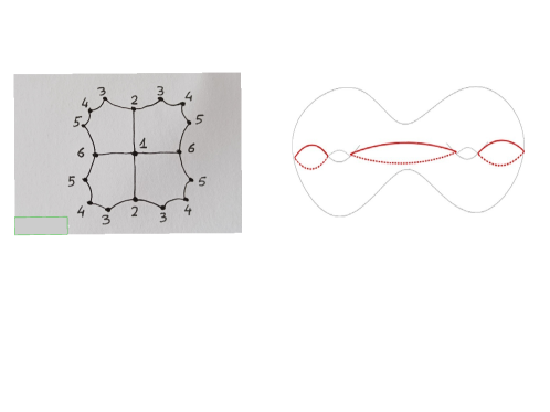
Figure 7. Up to repetition, there are only six vertices on the left side of this figure, which are the points $P_{i}$ indexed by $1,2,\dots,6$. They are located on the $x$-axis of the figure on the right. The hyperelliptic involution is a $180$-degree rotation around this axis. Three systoles are located on the vertical plane and the other three are on the horizontal plane.

7.3 An exemple of genus $17$.

When $2k=4$, the analysis is more complicated. We will describe a surface of genus $17$ endowed with a $4$-regular tesselation.

Let $H\subset W$ be the normal subgroup generated by the elements $(s_{i}s_{i+3})^{2}$ and set $S_{17}=\mathbb{H}/H$. The quotient $\Gamma:=W/H$ is isomorphicto $(\mathbb{Z}/2\mathbb{Z})^{6}$, hence $S_{17}$ is tesselated by $64$ hexagons. It follows that $S_{17}$ has genus $17$.

Lemma 19.

The systoles of $S_{17}$ are exactly the curves of the given tesselation.

Proof.

This specific example does not fully satisfies the hypotheses of criterion 18 of [10], so we will briefly explain the proof.

The group $\Gamma$ is given with $6$ generators, and its Caley graph $\mathrm{Cay}\,\Gamma$ is the one-skeleton of a $6$-dimensional cube. There is an embedding of $\mathrm{Cay}\,\Gamma$ in $S_{17}$. The vertices are the centers of the hexagons and the edges are the geodeosic arcs connecting two vertices belonging to two adjacent faces and crossing their common edge.

A loop in $\mathrm{Cay}\,\Gamma$ is a word $w$ on the letters $(s_{i})_{i\in\mathbb{Z}/6\mathbb{Z}}$ representing $1$ in $\Gamma$. The letters $s_{1},s_{3}$ and $s_{5}$ are called the red letters, and the other three are called the blue letters. For any word $w$, let $l_{R}(w)$, resp. $l_{B}(w)$, be the number of occurences of red letters, resp. of blue letters. Also set $l(w)=l_{R}(w)+l_{B}(w)$.

As in Lemma 14 of [10], any closed geodesic $\gamma$ is freely homotopic to a loop $\omega(\gamma)$ in $\mathrm{Cay}\,\Gamma$. Indeed if $\gamma$ crosses sucessively some edges of index $i_{1}$, $i_{2}$, $\dots i_{n}$ then $\omega(\gamma)$ is the word $s_{i_{1}}s_{i_{2}}\dots s_{i_{n}}$. If at some point $\gamma$ crosses a vertex at the intersection of two edges of indices $i$ and $i+1$, the previous definition is ambiguous. By convention, we will consider that $\gamma$ crosses first an edge of index $i$ and then an edge of index $i+1$.

We claim that the systoles of $S_{17}$ are the curves of the tesselation, which have length $4L$, where $L=\mathrm{arcosh}\,2$. Let $\gamma$ be a closed geodesic. Note that $l_{R}(\omega(\gamma)$ and $l_{B}(\omega(\gamma)$ are even.

First assume that $l(\omega(\gamma)>4$. We have $l_{R}(\omega(\gamma)\geq 4$ or $l_{B}(\omega(\gamma)\geq 4$ and $\gamma$ is not a curve of the tesselation. Therefore $\gamma$ has length bigger that $4L$ by Lemma 17 of [10].

Next assume that $l(\omega(\gamma)\leq 4$ It is obvious that $l(\omega(\gamma)$ is bigger than $2$, so we have $l(\omega(\gamma))=4$.

Note that $\omega(\gamma)$ cannot contains two identical consecutive letters, so $\omega(\gamma)=s_{i}s_{j}s_{i}s_{j}$ for some $i\neq j$. Note also that the words $s_{i}s_{i+1}s_{i}s_{i+i}$ are null-homotopic in $S_{17}$. If $\omega(\gamma)=s_{i}s_{i+2}s_{i}s_{i+2}$, then $\gamma$ is a curve of the tesselation. If $\omega(\gamma)=s_{i}s_{i+3}s_{i}s_{i+3}$, then $\gamma$ is a concatenation of four arcs which connects the middles of a side of index $i$ to a side of index $i+3$. If $c$ is one of these arcs, it cut an hexagon into two right-angled pentagons. By the formula of Theorem 3.5.10 of [14], we have $l(c)=\mathrm{arcosh}3$, therefore $l(\gamma)=4\mathrm{arcosh}3$ is bigger than $4L$. Since $\gamma$ is defined up to an orientation, we have treated all cases where $l(\omega(\gamma))=4$. ∎

The next lemma shows $\mathrm{codim}\,{\mathcal{P}}_{g}<2g-1$ for $g=17$.

Lemma 20.

We have $\mathrm{codim}\,{\mathcal{P}}_{17}<33$.

Proof.

The surface $S_{17}$ has $48$ curves. Let ${\mathcal{C}}$ be the set of all curves of index 3,4,5, or 6. As in the proof of Theorem 1, the set ${\mathcal{C}}$ fills the surface. Since $\mathrm{Card\,}{\mathcal{C}}=32$, we have $\mathrm{codim}\,{\mathcal{P}}_{17}<32$ by Corollary 18. ∎

Remark. The set ${\mathcal{C}}$ of the proof is not a minimal filling subset. Intuitive computations suggest that the minimal filling subsets have cardinality $25$, and that $\mathrm{codim}\,{\mathcal{P}}_{17}=24$.

References

[1]
O. Bolza.
On binary sextics with linear transformations between themselves.
Amer. J. Math., 10:47–70, 1888.
[2]
M. Fortier Bourque.
Hyperbolic surfaces with sublinearly many systoles that fill.
Commentarii Mathematici Helvetici, 95:515–534, 2020.
[3]
M. Fortier Bourque.
The dimension of Thurston’s spine.
Int. Math. Res. Not., pages 1–10, 2023.
[4]
M. Bridson and K. Vogtmann.
Automorphism groups of free groups, surface groups and free abelian
groups.
In Problems on mapping class groups and related topics,,
volume 74 of Proceedings of Symposia in Pure Mathematics, pages
301–316. American Mathematical Society, 2006.
[5]
P. Buser.
Geometry and Spectra of Compact Riemann Surfaces,
volume 106 of Progress in Mathematics.
Birkhäuser, 1992.
[6]
B. Farb and D. Margalit.
A primer on mapping class groups, volume 49 of Princeton
Mathematical Series.
Princeton University Press, Princeton, NJ, 2012.
[7]
J. Harer.
The virtual cohomological dimension of the mapping class group of an
orientable surface.
Inventiones Mathematicae, 84:157–176, 1986.
[8]
I. Irmer.
An explicit deformation retraction of the genus 2 moduli space.
To appear.
[9]
I. Irmer.
The differential topology of the Thurston spine.
arXiv:2211.03429, 2022.
[10]
I. Irmer and O. Mathieu.
Small systole sets and Coxeter groups.
Preprint, 2023.