An Optimal Ansatz Space for
Moving Least Squares Approximation on Spheres

Abstract

We revisit the moving least squares (MLS) approximation scheme on the sphere $\mathbb{S}^{d-1}\subset{\mathbb{R}}^{d}$, where $d>1$. It is well known that using the spherical harmonics up to degree $L\in{\mathbb{N}}$ as ansatz space yields for functions in $C^{L+1}(\mathbb{S}^{d-1})$ the approximation order ${\mathcal{O}}\left(h^{L+1}\right)$, where $h$ denotes the fill distance of the sampling nodes.

In this paper we show that the dimension of the ansatz space can be almost halved, by including only spherical harmonics of even or odd degree up to $L$, while preserving the same order of approximation. Numerical experiments indicate that using the reduced ansatz space is essential to ensure the numerical stability of the MLS approximation scheme as $h\xrightarrow{\ \ }0$. Finally, we compare our approach with an MLS approximation scheme that uses polynomials on the tangent space as ansatz space.

Introduction

Spherical data appears in many different scientific applications, such as geography and geodesy, astronomy, computer graphics and even in biology in protein docking simulation. This explains the need for fast and stable algorithms for the reconstruction of spherical functions from discrete data.

One approach is to use spherical harmonics up to a fixed degree as global ansatz space and to determine the coefficients by minimizing some error functional, see e.g. [1]. The choice of the polynomial degree as well as of the error functional are crucial to ensure the stability of the approximation process [7, 13, 8]. A second issue is the efficient numerical solution of the minimization problem which has been tackled, e.g., with the fast nonequispaced spherical Fourier transform [18, 12] or the double Fourier sphere method [16, 15]. A completely different approach are local approximation schemes, where many local approximations are computed instead of one global one. This avoids the costly solution of a large system of equations and stability can be resolved locally. Radial basis function approximation is a method that can be applied in a global schema [9, 11] as well as in a local one [10].

In this paper we revisit the moving least squares (MLS) approximation schema [14, 20, 22, 23] on the Euclidean sphere which is a purely local method. Assume that $f\colon{\mathbb{S}}^{d-1}\xrightarrow{\ \ }{\mathbb{C}}$ is a function from the $d-1$ dimensional sphere ${\mathbb{S}}^{d-1}=\{y\in{\mathbb{R}}^{d}\mid\lVert y\rVert=1\}$ to the complex numbers with known values on the nodes $y_{1},\dots,y_{N}\in{\mathbb{S}}^{d-1}$. Let $w\colon{\mathbb{S}}^{d-1}\times{\mathbb{S}}^{d-1}\xrightarrow{\ \ }{\mathbb{R}}_{\geq 0}$ denote a weight function and let ${\mathcal{G}}\subset{\mathcal{C}}\left({\mathbb{S}}^{d-1}\right)$ be a finite dimensional, linear ansatz space over ${\mathbb{C}}$. Under mild assumptions, cf. [14], there exists a unique function $g_{y}\in{\mathcal{G}}$ solving the weighted least squares problem

$$\min\limits_{g\in{\mathcal{G}}}\sum\limits_{i=1}^{N}w(y_{i},y)|f(y_{i})-g(y_{i})|^{2}.$$ (1)

The ansatz space ${\mathcal{G}}$ is usually chosen very low dimensional, which allows the weight function $w(\cdot,y)$ to be localized around $y\in\Omega$ with only few nodes $y_{i}$ close to the center $y$ satisfying $w(y_{i},y)>0$. As a result $g_{y}$ is only a local approximation to $f$ that is very fast to compute. In order to guarantee the stable solution of (1), the weight function needs to be carefully adapted to the nodes $y_{i}$ and the function space ${\mathcal{G}}$.

The MLS approximation ${\mathcal{M}}f(y)$ of $f$ is obtained by solving the local minimization problem (1) separately for each evaluation point $y\in\Omega$ and setting ${\mathcal{M}}f(y)\coloneqq g_{y}(y)$. An overview on the properties of the MLS approximation can be found in [6, chapter 22-25] and in [14].

In our paper we consider the asymptotic behavior of the approximation error

$$\|f-{\mathcal{M}}f\|_{\infty}=\sup\limits_{y\in{\mathbb{S}}^{d-1}}|f(y)-{\mathcal{M}}f(y)|$$ (2)

of the MLS approximation as the number $N$ of nodes increases, which simultaneously allows the weight function $w$ to become more and more localized. In order to bound the approximation error (2), the nodes $y_{i}$ need to be distributed sufficiently homogeneous in $\Omega$. The homogeneity of the nodes can be quantified by the ratio of their separation distance $q$ and their fill distance $h$, see Definition 4.2, which refer to the smallest distance between two nodes and the radius of the biggest hole, respectively. For $\Omega\subset{\mathbb{R}}^{d}$ it is well known, cf. [14, 22], that for $f\in C^{L+1}(\Omega)$ and $h\xrightarrow{\ \ }0$ we have $\|f-{\mathcal{M}}f\|_{\infty}={\mathcal{O}}\left(h^{L+1}\right)$, if the homogeneity $h/q$ is bounded by some constant $c$ and ${\mathcal{G}}$ consists of all polynomials up to degree $L$.

A similar result for ${\mathbb{S}}^{d-1}$ was shown by Wendland [23]. In his work he proved the asymptotic bound $\|f-{\mathcal{M}}f\|_{\infty}={\mathcal{O}}\left(h^{L+1}\right)$ whenever $f\in C^{L+1}({\mathbb{S}}^{d-1})$ and ${\mathcal{G}}$ consists of all spherical harmonics up to degree $L$.

In our paper we are going to show, that the dimension of the ansatz space ${\mathcal{G}}$ can be almost halved while preserving the same order of approximation. To be precise, if $L$ is even it will be sufficient to only use the spherical harmonics of even degree up to $L$, and if $L$ is odd it will be sufficient to only use the spherical harmonics of odd degree up to $L$, in order to obtain approximation order ${\mathcal{O}}\left(h^{L+1}\right)$ for $h\xrightarrow{\ \ }0$. This is possible, because the spherical harmonics up to degree $L$ are linearly independent from a global point of view, but they asymptotically become linearly dependent on a local scale. This is not the case anymore if we use only spherical harmonics of every second degree. Therefore, the smaller ansatz space also increases the numerical stability.

An alternative idea to keep the ansatz space ${\mathcal{G}}$ well suited for approximation problems that are more and more localized around some center $y$, is to allow it to vary with $y$ as well, i.e. to solve (1) with respect to a local ansatz space ${\mathcal{G}}_{y}$. A natural choice for such an ansatz space are the projections of the polynomials on the tangent space of the sphere at the center $y$ onto the sphere. This approach was already discussed for general manifolds in [20]. We show, that this method possesses the same approximation order ${\mathcal{O}}\left(h^{L+1}\right)$ for $h\xrightarrow{\ \ }0$ as our global ansatz space.

Our findings are organized as follows. In section 2 we give a quick introduction into moving least squares approximation. The essential point is that the approximation error can be bounded by the product of some Lebesgue constant and the error of the local best approximation, cf. Theorem 2.5. Local approximation on the sphere is discussed in section 3. In particular, we prove in LABEL:lem:Phi(G)_=_all_polynomials_up_to_degreeL conditions on the ansatz space $\mathcal{G}$, that guarantee that the error of the local best approximation of a function $f\in C^{L+1}({\mathbb{S}}^{d-1})$ within a $\delta$-ball around $y$ decays as $\mathcal{O}(\delta^{L+1})$. Subsequently, we show that these conditions are satisfied by the spaces of spherical harmonics of even, respectively odd, degree up to $L$ and summarize in Theorem 3.9 the local approximation properties of both spaces.

Section 4 is devoted to the computation of the Lebesgue constant for the spaces of spherical harmonics of even, respectively odd, degree up to $L$ generalizing a result of Wendland, cf. [23]. In Theorem 4.5 we give conditions on the separation distance and on the fill distance of the nodes $y_{i}$, as well as on the localization of the weight function $w$, such that the Lebesgue constant is uniformly bounded. Combining all these ingredients we end up with our final approximation result in Corollary 4.6.

Section 5 considers the case of a local ansatz space $\mathcal{G}_{y}$, which consists of the projections of polynomials on the tangent space onto the sphere. The two important factors, namely the error of the local best approximation and the Lebesgue constant, are estimated in Lemma 5.2 and LABEL:lem:tangent_lebesgueconstant_bounded, respectively. The final approximation result can be found in Corollary 5.4.

Eventually, in section 6, we numerically compare the three choices of the ansatz space: all spherical harmonics up to degree $L$, only the even, respectively odd, spherical harmonics up to degree $L$, and all polynomials up to degree $L$ on the tangent space of the sphere. Our numerical experiments indicate, that while all three approaches attain the approximation error proven in this paper, the latter two approaches result in much more stable algorithms, especially if the basis is chosen carefully.

Moving Least Squares Approximation

We start by giving an explicit definition of moving least squares approximation which dates back to Shepard [19].

Definition 2.1.

Let a function $f\colon{\mathbb{S}}^{d-1}\xrightarrow{\ \ }{\mathbb{C}}$ and a center $y\in{\mathbb{S}}^{d-1}$ be given. Further, let $y_{1},\dots,y_{N}\in{\mathbb{S}}^{d-1}$ be nodes, ${\mathcal{G}}=\operatorname{span}\left\{g_{1},\dots,g_{M}\colon{\mathbb{S}}^{d-1}\xrightarrow{\ \ }{\mathbb{R}}\right\}$ a linear ansatz space over ${\mathbb{C}}$ and $w\colon{\mathbb{S}}^{d-1}\times{\mathbb{S}}^{d-1}\xrightarrow{\ \ }{\mathbb{R}}_{\geq 0}$ a weight function, such that the minimization problem

$$\min\limits_{g\in{\mathcal{G}}}\,\sum\limits_{i=1}^{N}w(y,y_{i})\,|f(y_{i})-g(y_{i})|^{2}$$ (3)

possesses a unique solution $g_{y}\in{\mathcal{G}}$. Then ${\mathcal{M}}f(y)\coloneqq g_{y}(y)$ is the MLS approximation of $f$ in $y$.

Remark 2.2.

Of course the ansatz space ${\mathcal{G}}$ can be chosen as a linear space over ${\mathbb{R}}$ instead of ${\mathbb{C}}$ if $f$ is real-valued. Throughout the paper we will not distinguish between both cases. The ansatz space and all polynomial spaces defined throughout this paper should always be seen as linear spaces over the same field that $f$ maps into.

It is easy to check that the solution of (3) exists and is unique, if and only if the nodes $\left\{y_{i}\,\big{|}\,w(y_{i},y)>0\right\}$ are unisolvent with respect to ${\mathcal{G}}$, that is $g\equiv 0$ is the only function in ${\mathcal{G}}$ that vanishes on all these nodes. In this case, the MLS approximation coincides with the Backus-Gilbert approximation [3, 4]. For a proof of the following theorem see [14, Prop. 1].

Theorem 2.3 (Backus-Gilbert Approximation).

The MLS approximation can be written as

$${\mathcal{M}}f(y)=\sum_{w(y_{i},y)>0}a_{i}^{\ast}(y)f(y_{i}),$$ (4)

where the coefficients $a_{i}^{\ast}(y)\in{\mathbb{C}}$ are the unique solution of the minimization problem

$$\min\limits_{a_{i}(y)\in{\mathbb{C}}}\sum\limits_{w(y_{i},y)>0}\frac{1}{w(y_{i},y)}|a_{i}(y)|^{2}$$ (5)

subject to $$\sum\limits_{w(y_{i},y)>0}a_{i}(y)\,g(y_{i})=g(y)\quad,\,g\in{\mathcal{G}}.$$ (6)

From (6) we immediately conclude that ${\mathcal{M}}f=f$ for all $f\in{\mathcal{G}}$. This formulation of the MLS approximation is also called the Backus-Gilbert approximation and enables us to state an explicit upper bound for the error of the MLS approximation. This upper bound will depend on the error of the local best approximation of $f$.

Lets us first introduce some notations. The distance between two points $y,z\in{\mathbb{S}}^{d-1}$ on the sphere is measured via the great circle distance

$$d(y,z)=\arccos\left(\langle y,z\rangle\right),$$

where $\langle y,z\rangle=y_{1}z_{1}+\dots+y_{d}z_{d}$ denotes the euclidean inner product on ${\mathbb{R}}^{d}$. The open spherical cap $C_{\delta}(y)$ with radius $\delta>0$ around the center $y\in{\mathbb{S}}^{d-1}$ is defined as

$$C_{\delta}(y)\coloneqq\left\{z\in{\mathbb{S}}^{d-1}\,\middle|\,d(y,z)<\delta\right\}.$$

Definition 2.4.

Let $f\colon{\mathbb{S}}^{d-1}\xrightarrow{\ \ }{\mathbb{C}}$ be a spherical function, $y\in{\mathbb{S}}^{d-1}$ and $\delta>0$. Then the error of the local best approximation of $f$ from ${\mathcal{G}}$ on the spherical cap $C_{\delta}(y)$ is defined as

$$E_{\delta}({\mathcal{G}},f,y)\coloneqq\inf\limits_{g\in{\mathcal{G}}}\sup\limits_{z\in C_{\delta}(y)}|f(z)-g(z)|$$ (7)

A proof of the following theorem can be found in [6, 14].

Theorem 2.5.

Let ${\mathcal{M}}f(y)$ be the MLS approximation of $f$ in $y\in{\mathbb{S}}^{d-1}$ and let

$$\delta\coloneqq\max\limits_{w(y_{i},y)>0}d(y_{i},y)$$

denote the largest distance to the center $y$ among all nodes with positive weight. The error of the MLS approximation is bounded by

$$|f(y)-{\mathcal{M}}f(y)|\leq E_{\delta}({\mathcal{G}},f,y)\left(1+\sum\limits_{w(y_{i},y)>0}|a_{i}^{\ast}(y)|\right).$$ (8)

The sum $\sum_{w(y_{i},y)>0}|a_{i}^{\ast}(y)|$ is called the Lebesgue constant. As the number of nodes $N$ goes to infinity we can make the weight function more localized, so that simultaneously $\delta$ approaches $0$ in the above theorem. It is easy to check, that $\delta\xrightarrow{\ \ }0$ also implies $E_{\delta}({\mathcal{G}},f,y)\xrightarrow{\ \ }0$ and the error $|{\mathcal{M}}f(y)-f(y)|$ inherits this decay if at the same time the Lebesgue constant remains bounded. In the following section we will find for every $L\in{\mathbb{N}}_{0}$ an ansatz space ${\mathcal{G}}$, such that $E_{\delta}({\mathcal{G}},f,y)={\mathcal{O}}\left(\delta^{L+1}\right)$ for $\delta\xrightarrow{\ \ }0$. In section 4 we give sufficient conditions on the weight function and on the nodes, which guarantee that the Lebesgue constant is uniformly bounded for all centers $y\in{\mathbb{S}}^{d-1}$. Overall this will give the desired approximation order $\|{\mathcal{M}}f-f\|_{\infty}={\mathcal{O}}\left(\delta^{L+1}\right)$ of the MLS approximation.

A Minimal Ansatz Space for Local Approximation on Spheres

The goal of this section is to find for given $L\in{\mathbb{N}}_{0}$ an ansatz space ${\mathcal{G}}\subset{\mathcal{C}}^{\infty}({\mathbb{S}}^{d-1})$, such that for all functions $f\in{\mathcal{C}}^{L+1}({\mathbb{S}}^{d-1})$ and centers $y\in{\mathbb{S}}^{d-1}$ the error of the local best approximation of $f$ on the spherical cap $C_{\delta}(y)$ with functions from ${\mathcal{G}}$ decays with order ${\mathcal{O}}\left(\delta^{L+1}\right)$ for $\delta\xrightarrow{\ \ }0$, i.e.

$$E_{\delta}\left({\mathcal{G}},f,y\right)={\mathcal{O}}\left(\delta^{L+1}\right).$$ (9)

Additionally the dimension of ${\mathcal{G}}$ should be as small as possible.

Our idea is to utilize Taylor series to obtain the desired result. This requires a local projection between the sphere ${\mathbb{S}}^{d-1}$ and its tangent space ${\mathbb{R}}^{d-1}$. Thanks to symmetry it will be sufficient to only consider the projection around the north pole $e_{d}=(0,\dots,0,1)\in{\mathbb{S}}^{d-1}$.

Definition 3.1.

The orthogonal projection from the open ball $B_{1}(\bm{0})\subset{\mathbb{R}}^{d-1}$ with radius $1$ around $\bm{0}\in{\mathbb{R}}^{d-1}$ onto the open spherical cap $C_{\frac{\pi}{2}}(e_{d})\subset{\mathbb{S}}^{d-1}$ with radius $\frac{\pi}{2}$ around the north pole $e_{d}\in{\mathbb{S}}^{d-1}$ is defined as

$$\pi\colon B_{1}(\bm{0})\xrightarrow{\ \ }C_{\frac{\pi}{2}}(e_{d}),\,(x_{1},\dots,x_{d-1})\mapsto\left(x_{1},\dots,x_{d-1},\sqrt{1-\|x\|_{2}^{2}}\right).$$ (10)

It is easy to check that this projection is bijective with inverse

$$\pi^{-1}\colon C_{\frac{\pi}{2}}(e_{d})\xrightarrow{\ \ }B_{1}(\bm{0}),\,(y_{1},\dots,y_{d})\mapsto(y_{1},\dots,y_{d-1}).$$ (11)

For a given function $f\in{\mathcal{C}}({\mathbb{S}}^{d-1})$, the projection $\pi$ naturally defines the pullback function

$$f^{\ast}\coloneqq{f}\circ{}{\pi}\colon B_{1}(\bm{0})\xrightarrow{\ \ }{\mathbb{C}},$$

which possesses the same order of differentiability as $f$ itself. Indeed, for $f\in{\mathcal{C}}^{L}({\mathbb{S}}^{d-1})$ we obtain

$$f^{\ast}(x)=f\circ\pi(x)=f\left(x_{1},\dots,x_{d-1},\sqrt{1-\|x\|_{2}^{2}}\right)$$

and the variable substitution $x_{d}\mapsfrom\sqrt{1-\|x\|_{2}^{2}}$ does not affect the order of differentiability for $x\in B_{1}(\bm{0})$. This allows us to utilize the Taylor series of the pullback function $f^{\ast}$ as a substitute of the Taylor series of $f$ itself. To this end we denote by

$$\operatorname{Hom}_{\ell}({\mathbb{R}}^{d})=\operatorname{span}\left\{\bm{x}^{\bm{\alpha}}\colon{\mathbb{R}}^{d}\xrightarrow{\ \ }{\mathbb{R}},\,x\mapsto\prod\limits_{i=1}^{d}x_{i}^{\alpha_{i}}\,\middle|\,\bm{\alpha}\in{\mathbb{N}}_{0}^{d},\,|\bm{\alpha}|=\alpha_{1}+\dots+\alpha_{d}=\ell\right\}.$$

the space of homogeneous polynomials of degree $\ell\in{\mathbb{N}}_{0}$ on ${\mathbb{R}}^{d}$. The dimension is given by

$$\dim\left(\operatorname{Hom}_{\ell}({\mathbb{R}}^{d-1})\right)=\binom{d-1+\ell}{\ell},$$ (12)

see [5, Proposition 4.2]. Further we denote their direct sum up to degree $L\in{\mathbb{N}}_{0}$ by

$${\mathcal{P}}_{L}({\mathbb{R}}^{d-1}):=\bigoplus_{\ell=0}^{L}\operatorname{Hom}_{\ell}({\mathbb{R}}^{d-1})$$

Definition 3.2.

For $L\in{\mathbb{N}}_{0}$ we define the mapping

$$T_{L}\colon{\mathcal{C}}^{L}({\mathbb{S}}^{d-1})\xrightarrow{\ \ }{\mathcal{P}}_{L}({\mathbb{R}}^{d-1}),\,f\mapsto T_{L}\left(f\right)=\sum\limits_{\bm{\alpha}\in{\mathbb{N}}_{0}^{d-1},\,|\bm{\alpha}|\leq L}\frac{\left(f^{\ast}\right)^{(\bm{\alpha})}(\bm{0})}{\bm{\alpha}!}\bm{x}^{\bm{\alpha}},$$

that maps every function $f\in{\mathcal{C}}^{L}({\mathbb{S}}^{d-1})$ to the Taylor series of order $L$ of its pullback $f^{\ast}={f}\circ{}{\pi}$.

Note, that the truncated Taylor series $T_{L}(g)$ of arbitrary degree $L\in{\mathbb{N}}_{0}$ is well defined for all ansatz functions $g\in{\mathcal{G}}\subset{\mathcal{C}}^{\infty}({\mathbb{S}}^{d-1})$. Investigating the image $T_{L}({\mathcal{G}})\subset{\mathcal{P}}_{L}({\mathbb{R}}^{d-1})$ allows us to state a sufficient condition, which ensures that the error $E_{\delta}({\mathcal{G}},f,y)$ of the local best approximation decays with order ${\mathcal{O}}\left(\delta^{L+1}\right)$ for $\delta\xrightarrow{\ \ }0$.

Lemma 3.3.

Let $L\in{\mathbb{N}}_{0}$ be given and let ${\mathcal{G}}\subset{\mathcal{C}}^{\infty}({\mathbb{S}}^{d-1})$ be an ansatz space, such that

1. ${\mathcal{G}}$ is rotational invariant, i.e. $\left\{g\circ\bm{R}\,\middle|\,g\in{\mathcal{G}}\right\}={\mathcal{G}}$ for all rotation matrices $\bm{R}\in\mathcal{SO}(d)$ and

2. every $p\in{\mathcal{P}}_{L}({\mathbb{R}}^{d-1})$ is the Taylor series of the pullback function $g^{\ast}$ of some $g\in{\mathcal{G}}$, i.e.

   $$T_{L}\left({\mathcal{G}}\right)={\mathcal{P}}_{L}({\mathbb{R}}^{d-1}).$$ (13)

Then for all $f\in{\mathcal{C}}^{L+1}({\mathbb{S}}^{d-1})$ and $y\in{\mathbb{S}}^{d-1}$ the error $E_{\delta}({\mathcal{G}},f,y)$ of the local best approximation of $f$ from the ansatz space ${\mathcal{G}}$ on the spherical cap $C_{\delta}(y)$ vanishes with order $L+1$ as $\delta$ goes to $0$:

$$E_{\delta}({\mathcal{G}},f,y)={\mathcal{O}}(\delta^{L+1}).$$

Proof.

First we prove the statement in the north pole $y=e_{d}$. To this end let $f\in{\mathcal{C}}^{L+1}({\mathbb{S}}^{d-1})$ be given. By assumption 2), there exists a function $g\in{\mathcal{G}}$, such that $T_{L}(g)=T_{L}(f)$. We show, that $g$ locally approximates $f$ with order ${\mathcal{O}}\left(\delta^{L+1}\right)$ as $\delta$ goes to zero.

For $\delta\xrightarrow{\ \ }0$ we may assume $\delta<\frac{\pi}{2}$, so that the inverse projection ${\pi}^{-1}(y)$ is well defined for all $y\in C_{\delta}(e_{d})$. Let us choose $y\in C_{\delta}(e_{d})$ and set $x\coloneqq\pi^{-1}(y)$. From $y\in C_{\delta}(e_{d})$ we obtain $y_{d}>\cos\delta$ and the definition of the projection $\pi$ yields:

$$\|x\|_{2}^{2}=y_{1}^{2}+\dots+y_{d-1}^{2}=1-y_{d}^{2}<1-\cos^{2}\delta=\sin^{2}\delta.$$

Thus $x$ is contained in the ball $B_{\sin\delta}(\bm{0})$ with radius $\sin\delta$ around the center $\bm{0}$. Using the Taylor series of order $L\in{\mathbb{N}}_{0}$ and the corresponding remainder term, we can write the pullback function $f^{\ast}(x)=f\circ\pi(x)$ as

$$f^{\ast}(x)=\left(T_{L}(f)\right)(x)+\sum\limits_{\bm{\alpha}\in{\mathbb{N}}_{0}^{d-1},\,|\bm{\alpha}|=L+1}\frac{\left(f^{\ast}\right)^{(\bm{\alpha})}(\xi_{f,x})}{\bm{\alpha}!}\bm{x}^{\bm{\alpha}}$$

with some $\xi_{f,x}\in B_{\sin\delta}(\bm{0})$, that depends on the function $f$ and the point $x$. The same can be applied to $g$. Because of $T_{L}(f)=T_{L}(g)$ this yields for all $y\in C_{\delta}(e_{d})$:

$$\left|f(y)-g(y)\right|=\left|f^{\ast}(x)-g^{\ast}(x)\right|=\left|\sum\limits_{\bm{\alpha}\in{\mathbb{N}}_{0}^{d-1},\,|\bm{\alpha}|=L+1}\frac{(f^{\ast})^{(\bm{\alpha})}(\xi_{f,x})-(g^{\ast})^{(\bm{\alpha})}(\xi_{g,x})}{\bm{\alpha}!}\bm{x}^{\bm{\alpha}}\right|.$$

Since $x\in B_{\sin\delta}(\bm{0})$, each component of $x$ is bounded by $\sin\delta$ and hence $|\bm{x}^{\bm{\alpha}}|\leq\sin^{L+1}(\delta)$. Further

$$K:=\sup\limits_{x\in B_{\sin\delta}(\bm{0})}\sum\limits_{\bm{\alpha}\in{\mathbb{N}}_{0}^{d-1},\,|\bm{\alpha}|=L+1}\left|\frac{{\left(f^{\ast}\right)}^{(\bm{\alpha})}(\xi_{f,x})-{\left(g^{\ast}\right)}^{(\bm{\alpha})}(\xi_{g,x})}{\bm{\alpha}!}\right|<\infty$$

because of $f,\,g\in{\mathcal{C}}^{L+1}({\mathbb{S}}^{d-1})$. This leads for $\delta\xrightarrow{\ \ }0$ to the error estimate

$$\sup\limits_{y\in C_{\delta}(e_{d})}|f(y)-g(y)|\leq K\,\sin^{L+1}(\delta)\leq K\,\delta^{L+1}$$

and since $K$ is decreasing as $\delta$ goes to zero this proves the statement for the north pole $e_{d}$. For general $y\in{\mathbb{S}}^{d-1}$ the statement follows from the rotational invariance of ${\mathcal{G}}$.

A well known ansatz space ${\mathcal{G}}$ that satisfies the conditions of Lemma 3.3 are the spherical polynomials

$${\mathcal{H}}_{L}({\mathbb{S}}^{d-1}):=\bigoplus_{\ell=0}^{L}\operatorname{Harm}_{\ell}({\mathbb{S}}^{d-1})$$

up to a certain degree $L\in{\mathbb{N}}$ where

$$\operatorname{Harm}_{\ell}({\mathbb{S}}^{d-1})=\left\{h\big{|}_{{\mathbb{S}}^{d-1}}\colon{\mathbb{S}}^{d-1}\xrightarrow{\ \ }{\mathbb{C}}\,\middle|\,h\in\operatorname{Hom}_{\ell}({\mathbb{R}}^{d}),\,\Delta_{d}(h)\equiv 0\right\},$$

denotes the harmonic space of degree $\ell\in{\mathbb{N}}$ and $\Delta_{d}$ the Laplace operator in $d$ dimensions. The elements of $\operatorname{Harm}_{\ell}({\mathbb{S}}^{d-1})$ are called spherical harmonics of degree $\ell$.

Let us collect some properties of the harmonic spaces. The dimension of one harmonic space is given by

$$\dim\left(\operatorname{Harm}_{\ell}({\mathbb{S}}^{d-1})\right)=\dim\left(\operatorname{Hom}_{\ell}({\mathbb{R}}^{d-1})\right)+\dim\left(\operatorname{Hom}_{\ell-1}({\mathbb{R}}^{d-1})\right),\,\ell\geq 1$$ (14)

and $\dim\left(\operatorname{Hom}_{0}({\mathbb{R}}^{d-1})\right)=1$ respectively, see [17, Equation 7]. By Theorem 5.7 from [2], every $p\in\operatorname{Hom}_{L}({\mathbb{R}}^{d})$ can be uniquely written as

$$p=h_{L}+\|x\|_{2}^{2}\,h_{L-2}+\dots+\|x\|_{2}^{L-\sigma}h_{\sigma},$$

where $\sigma\coloneqq L\mkern 4.0mu({\operator@font mod}\mkern 6.0mu2)$ and $h_{\ell}\in\operatorname{Hom}_{\ell}({\mathbb{R}}^{d})$ with $\Delta_{d}\,h_{\ell}=0,\,\ell=L,L-2,\dots,\sigma$. Restricting the above representation of $p$ to the sphere proves the following lemma.

Lemma 3.4.

For every monomial $\bm{x}^{\bm{\alpha}}\in\operatorname{Hom}_{L}({\mathbb{R}}^{d})$ of degree $L=|\bm{\alpha}|=\alpha_{1}+\dots+\alpha_{d}$

$$\bm{x}^{\bm{\alpha}}(x)=\prod\limits_{i=1}^{d}x_{i}^{\alpha_{i}},\quad x\in{\mathbb{R}}^{d}$$

there exist spherical harmonics $h_{\ell}\in\operatorname{Harm}_{\ell}({\mathbb{S}}^{d-1})$ of degree $\ell=L,L-2,\dots,\sigma\coloneqq L\mkern 4.0mu({\operator@font mod}\mkern 6.0mu2)$, such that the restriction of $\bm{x}^{\bm{\alpha}}$ to the sphere equals the sum of the spherical harmonics $h_{\ell}$:

$$\bm{x}^{\bm{\alpha}}(y)=h_{L}(y)+h_{L-2}(y)+\dots+h_{\sigma}(y),\quad y\in{\mathbb{S}}^{d-1}.$$

Using this lemma we can quickly verify that $T_{L}\left({\mathcal{H}}_{L}({\mathbb{S}}^{d-1})\right)={\mathcal{P}}_{L}({\mathbb{R}}^{d-1})$ and of course ${\mathcal{H}}_{L}({\mathbb{S}}^{d-1})$ inherits the rotational invariance from the harmonic spaces, hence $E_{\delta}({\mathcal{G}},f,y)={\mathcal{O}}\left(\delta^{L+1}\right)$ for all $f\in{\mathcal{C}}({\mathbb{S}}^{d-1})$ and for all $y\in{\mathbb{S}}^{d-1}$ as $\delta\xrightarrow{\ \ }0$ because of Lemma 3.3.

However, we also want the dimension of the ansatz space to be as small as possible. With respect to the condition $T_{L}\left({\mathcal{G}}\right)={\mathcal{P}}_{L}({\mathbb{R}}^{d-1})$ of LABEL:lem:Phi(G)_=_all_polynomialsup_to_degree_L, the dimension of the ansatz space is bounded from below by $\dim\left({\mathcal{G}}\right)\geq\dim\left({\mathcal{P}}_{L}({\mathbb{R}}^{d-1})\right)$. In comparison, from (14) we obtain

$$\dim\left({\mathcal{H}}_{L}({\mathbb{S}}^{d-1})\right)=\dim\left({\mathcal{P}}_{L}({\mathbb{R}}^{d-1})\right)+\dim\left({\mathcal{P}}_{L-1}({\mathbb{R}}^{d-1})\right),\,L\geq 1$$

and $\dim\left({\mathcal{H}}_{0}({\mathbb{S}}^{d-1})\right)=1$ respectively, which is almost twice as big as the lower bound.

We will now drastically reduce the dimension of the ansatz space by leaving out the harmonic spaces of every second degree and showing, that both conditions of LABEL:lem:Phi(G)_=_allpolynomials_up_to_degree_L remain satisfied.

Definition 3.5.

For $L\in{\mathbb{N}}_{0}$ we denote the direct sum of the harmonic spaces of even, respectively odd, degree up to $L$ by

$${\mathcal{H}}_{L,2}({\mathbb{S}}^{d-1})\coloneqq\bigoplus\limits_{\ell\leq L,\,\ell\equiv L\mkern 4.0mu({\operator@font mod}\mkern 6.0mu2)}\operatorname{Harm}_{\ell}({\mathbb{S}}^{d-1}).$$ (15)

We can use (14) to easily verify that the dimension of this new ansatz space even attains the lower bound with respect to Lemma 3.3:

$$\dim\left({\mathcal{H}}_{L,2}({\mathbb{S}}^{d-1})\right)=\dim\left({\mathcal{P}}_{L}({\mathbb{R}}^{d-1})\right).$$ (16)

Since ${\mathcal{H}}_{L,2}({\mathbb{S}}^{d-1})$ is the direct sum of harmonic spaces, it is still rotational invariant and thus we only have to show, that the condition $T_{L}\left({\mathcal{H}}_{L,2}({\mathbb{S}}^{d-1})\right)={\mathcal{P}}_{L}({\mathbb{R}}^{d-1})$ remains satisfied. To this end we introduce a basis of both ${\mathcal{H}}_{L,2}({\mathbb{S}}^{d-1})$ and ${\mathcal{P}}_{L}({\mathbb{R}}^{d-1})$. For the latter one, we utilize the monomial basis

$$\left\{\bm{x}^{\bm{\alpha}}\colon{\mathbb{R}}^{d-1}\xrightarrow{\ \ }{\mathbb{R}}\,\middle|\,\bm{\alpha}\in{\mathbb{N}}_{0}^{d-1},\,|\bm{\alpha}|\leq L\right\}.$$ (17)

The harmonic spaces are usually equipped with an $L^{2}$-orthogonal basis. However, for our purpose the following monomial basis of ${\mathcal{H}}_{L,2}({\mathbb{S}}^{d-1})$ is more suitable.

Lemma 3.6.

Let $L\in{\mathbb{N}}_{0}$ be given. The set of all $d$-variate monomials whose degree is less or equal to $L$ and has the same parity as $L$, and whose exponent in the last variable is $0$ or $1$

$${\mathcal{B}}_{L,2}\coloneqq\left\{\bm{y}^{\bm{\alpha}}\colon{\mathbb{S}}^{d-1}\xrightarrow{\ \ }{\mathbb{R}}\,\middle|\,\bm{\alpha}\in{\mathbb{N}}_{0}^{d},\,|\bm{\alpha}|\leq L,\,|\bm{\alpha}|\equiv L\mkern 4.0mu({\operator@font mod}\mkern 6.0mu2),\,\alpha_{d}\leq 1\right\}$$

is a basis of the even, respectively odd, harmonic spaces ${\mathcal{H}}_{L,2}({\mathbb{S}}^{d-1})$ up to degree $L$.

Proof.

First we are going to verify, that the number of elements in ${\mathcal{B}}_{L,2}$ equals the dimension of the space ${\mathcal{H}}_{L,2}({\mathbb{S}}^{d-1})$. After that we show, that ${\mathcal{H}}_{L,2}({\mathbb{S}}^{d-1})$ is the span of ${\mathcal{B}}_{L,2}$. Together this implies, that ${\mathcal{B}}_{L,2}$ is a basis of ${\mathcal{H}}_{L,2}({\mathbb{S}}^{d-1})$. For the first step, we count the elements in ${\mathcal{B}}_{L,2}$, which gives

$$\begin{split}|{\mathcal{B}}_{L,2}|&=\left|\left\{\bm{\alpha}\in{\mathbb{N}}_{0}^{d}\,\middle|\,|\bm{\alpha}|\leq L,\,|\bm{\alpha}|\equiv L\mkern 4.0mu({\operator@font mod}\mkern 6.0mu2),\,\alpha_{d}=0\right\}\right|\\ &\quad\hskip 85.35826pt+\left|\left\{\bm{\alpha}\in{\mathbb{N}}_{0}^{d}\,\middle|\,|\bm{\alpha}|\leq L,\,|\bm{\alpha}|\equiv L\mkern 4.0mu({\operator@font mod}\mkern 6.0mu2),\,\alpha_{d}=1\right\}\right|\\ &=\left|\left\{\widetilde{\bm{\alpha}}\in{\mathbb{N}}_{0}^{d-1}\,\middle|\,|\widetilde{\bm{\alpha}}|\leq L,|\widetilde{\bm{\alpha}}|\equiv L\mkern 4.0mu({\operator@font mod}\mkern 6.0mu2)\right\}\right|\\ &\quad\hskip 85.35826pt+\left|\left\{\widetilde{\bm{\alpha}}\in{\mathbb{N}}_{0}^{d-1}\,\middle|\,|\widetilde{\bm{\alpha}}|\leq L-1,\,|\widetilde{\bm{\alpha}}|\equiv L-1\mkern 4.0mu({\operator@font mod}\mkern 6.0mu2)\right\}\right|\\ &=\left|\left\{\widetilde{\bm{\alpha}}\in{\mathbb{N}}_{0}^{d-1}\,\middle|\,|\widetilde{\bm{\alpha}}|\leq L\right\}\right|=\dim\left({\mathcal{P}}_{L}({\mathbb{R}}^{d-1})\right)=\dim\left({\mathcal{H}}_{L,2}({\mathbb{S}}^{d-1})\right),\end{split}$$ (18)

where we used (16) in the last step.

For the second part of the proof we first note that $\operatorname{span}\left\{{\mathcal{B}}_{L,2}\right\}\subseteq{\mathcal{H}}_{L,2}({\mathbb{S}}^{d-1})$ by Lemma 3.4. For the other inclusion, let $h\in{\mathcal{H}}_{L,2}({\mathbb{S}}^{d-1})$ be given and denote $\sigma\coloneqq L\mod 2$. By the definition of ${\mathcal{H}}_{L,2}({\mathbb{S}}^{d-1})$ we may write $h=h_{L}+h_{L-2}+\dots+h_{\sigma}$ with $h_{\ell}\in\operatorname{Harm}_{\ell}({\mathbb{S}}^{d-1}),\,\ell=L,L-2,\dots,\sigma$. Further, by the definition of the harmonic spaces, there exist homogeneous polynomials $H_{\ell}\in\operatorname{Hom}_{\ell}({\mathbb{R}}^{d})$, such that $h_{\ell}=H_{\ell}\big{|}_{{\mathbb{S}}^{d-1}}$ for $\ell=L,L-2,\dots,\sigma$ and we may write the sum as

$$H\coloneqq H_{L}+H_{L-2}+\dots+H_{\sigma}=\sum\limits_{\bm{\alpha}\in{\mathbb{N}}_{0}^{d},\,|\bm{\alpha}|\leq L,\,|\bm{\alpha}|\equiv L\mkern 4.0mu({\operator@font mod}\mkern 6.0mu2)}c_{\alpha}\bm{y}^{\bm{\alpha}}$$

with coefficients $c_{\alpha}\in{\mathbb{C}}$. If the coefficients are $0$ for all monomials $\bm{y}^{\bm{\alpha}}$ with $\alpha_{d}\geq 2$ then there exists an element $g\in\operatorname{span}\left\{{\mathcal{B}}_{L,2}\right\}$ with $g=H\big{|}_{{\mathbb{S}}^{d-1}}=h$ and we are done. If not, we repeat substitution of the identity $y_{d}^{2}=1-y_{1}^{2}+\dots+y_{d}^{2}$

$$\bm{y}^{\bm{\alpha}}(y) =y_{1}^{\alpha_{1}}\cdot\dots\cdot y_{d}^{\alpha_{d}}=y_{1}^{\alpha_{1}}\cdot\dots\cdot y_{d-1}^{\alpha_{d-1}}y_{d}^{\alpha_{d}-2}\left(1-y_{1}^{2}-\dots-y_{d-1}^{2}\right)$$

$$=y_{1}^{\alpha_{1}}\cdot\dots\cdot y_{d-1}^{\alpha_{d-1}}y_{d}^{\alpha_{d}-2}-\sum\limits_{i=1}^{d-1}y_{i}^{2}\cdot y_{1}^{\alpha_{1}}\cdot\dots\cdot y_{d-1}^{\alpha_{d-1}}y_{d}^{\alpha_{d}-2},\,y\in{\mathbb{S}}^{d-1}$$

until the highest remaining exponent in the $d$-th variable is $1$ or $0$. Note that the value of $H$ remains unchanged on ${\mathbb{S}}^{d-1}$. Since the substitution always yields monomials of the same degree or $2$ less, the condition $|\bm{\alpha}|\leq L,\,|\bm{\alpha}|\equiv L\mkern 4.0mu({\operator@font mod}\mkern 6.0mu2)$ remains satisfied in all monomials $\bm{y^{\bm{\alpha}}}$ too. Hence there exists an element $g\in\operatorname{span}\left\{{\mathcal{B}}_{L,2}\right\}$ with $g=H\big{|}_{{\mathbb{S}}^{d-1}}=h$ and thus ${\mathcal{H}}_{L,2}\subseteq\operatorname{span}\left\{{\mathcal{B}}_{L,2}\right\}$.

Remark 3.7.

It is straightforward to see, that ${\mathcal{H}}_{L}({\mathbb{S}}^{d-1})={\mathcal{H}}_{L,2}({\mathbb{S}}^{d-1})\oplus{\mathcal{H}}_{L-1,2}({\mathbb{S}}^{d-1})$ and hence the union ${\mathcal{B}}_{L,2}\cup{\mathcal{B}}_{L-1,2}$ constitutes a monomial basis of ${\mathcal{H}}_{L}({\mathbb{S}}^{d-1})$. This basis has also been mentioned in [9].

The monomial basis ${\mathcal{B}}_{L,2}$ enables us to show, that the second condition of LABEL:lem:Phi(G)_=_all_polynomials_upto_degree_L is satisfied as well.

Lemma 3.8.

Let $L\in{\mathbb{N}}_{0}$ be given. The linear mapping

$$T_{L}\colon{\mathcal{H}}_{L,2}({\mathbb{S}}^{d-1})\xrightarrow{\ \ }{\mathcal{P}}_{L}({\mathbb{R}}^{d-1}),\quad g\mapsto\sum\limits_{\bm{\alpha}\in{\mathbb{N}}_{0}^{d-1},\,|\bm{\alpha}|\leq L}\frac{\left(g^{\ast}\right)^{(\bm{\alpha})}(\bm{0})}{\bm{\alpha}!}\bm{x}^{\bm{\alpha}},$$

that maps every function $g\in{\mathcal{H}}_{L,2}({\mathbb{S}}^{d-1})$ to the truncated Taylor series of order $L$ of the pullback function $g^{\ast}=g\circ\pi$ satisfies condition 2) of LABEL:lem:Phi(G)_=_allpolynomials_up_to_degree_L, i.e. $T_{L}\left({\mathcal{H}}_{L,2}({\mathbb{S}}^{d-1})\right)={\mathcal{P}}_{L}({\mathbb{R}}^{d-1})$.

Proof.

We equip ${\mathcal{H}}_{L,2}({\mathbb{S}}^{d-1})$ with the basis ${\mathcal{B}}_{L,2}$ from Lemma 3.6 and ${\mathcal{P}}_{L}({\mathbb{R}}^{d-1})$ with the monomial basis from (17). Let $\bm{M}_{L}=m_{L}^{\bm{\alpha},\bm{\beta}}$ denote the corresponding matrix representation of $T_{L}$, where $\bm{\alpha}\in{\mathbb{N}}_{0}^{d},\,|\bm{\alpha}|\leq L,\,|\bm{\alpha}|\equiv L\mkern 4.0mu({\operator@font mod}\mkern 6.0mu2),\,\alpha_{d}\leq 1$ and $\bm{\beta}\in{\mathbb{N}}_{0}^{d-1},\,|\bm{\beta}|\leq L$. From

$$T_{L}(\bm{y}^{\bm{\alpha}})=\sum\limits_{\bm{\beta}\in{\mathbb{N}}_{0}^{d-1},\,|\bm{\beta}|\leq L}\frac{\left(\bm{y}^{\bm{\alpha}}\circ\pi\right)^{(\bm{\beta})}(\bm{0})}{\bm{\beta}!}\bm{x}^{\bm{\beta}}$$

we can read off the matrix entries of $\bm{M}_{L}$:

$$m_{L}^{\bm{\alpha},\bm{\beta}}=\frac{\left(\bm{y}^{\bm{\alpha}}\circ\pi\right)^{(\bm{\beta})}(\bm{0})}{\bm{\beta}!}.$$ (19)

Let $\bm{y}^{\bm{\alpha}}\in{\mathcal{B}}_{L,2}$ be a basis element and denote $\widetilde{\bm{\alpha}}:=(\alpha_{1},\dots,\alpha_{d-1})\in{\mathbb{N}}_{0}^{d-1}$ and $\bm{\alpha}=(\widetilde{\bm{\alpha}},\alpha_{d})$. Recall that, by the definition of ${\mathcal{B}}_{L,2}$, the multi-index $\bm{\alpha}$ satisfies $\alpha_{d}\in\{0,1\}$. We are going to compute $m_{L}^{\bm{\alpha},\bm{\beta}}$ for $\alpha_{d}=0$ and $\alpha_{d}=1$ separately.

First we consider $\alpha_{d}=0$. For $x\in B_{1}(\bm{0})$ the pullback of the basis element $\bm{y}^{(\widetilde{\bm{\alpha}},0)}\in{\mathcal{B}}_{L,2}$ can be written as

$$\bm{y}^{(\widetilde{\bm{\alpha}},0)}\circ\pi(x)=\bm{y}^{(\widetilde{\bm{\alpha}},0)}(x_{1},\dots,x_{d-1},\sqrt{1-\|x\|_{2}^{2}})=\left(x_{1},\dots,x_{d-1}\right)^{\widetilde{\bm{\alpha}}}=x^{\widetilde{\bm{\alpha}}},$$

hence $\bm{y}^{(\widetilde{\bm{\alpha}},0)}\circ\pi=\bm{x}^{\bm{\widetilde{\alpha}}}$ on $B_{1}(\bm{0})$. In order to evaluate the matrix entry (19), we have to take the derivative with respect to some $\bm{\beta}\in{\mathbb{N}}_{0}^{d-1},\,|\bm{\beta}|\leq L$ and evaluate it in the point $\bm{0}\in{\mathbb{R}}^{d-1}$. Since the evaluation of any non-constant monomial in the point $\bm{0}\in{\mathbb{R}}^{d-1}$ always gives $0$, we get

$$m_{L}^{(\widetilde{\bm{\alpha}},0),\bm{\beta}}=\frac{\left(\bm{y}^{(\widetilde{\bm{\alpha}},0)}\circ\pi\right)^{(\bm{\beta})}(\bm{0})}{\bm{\beta}!}=\frac{\left(\bm{x}^{\widetilde{\bm{\alpha}}}\right)^{(\bm{\beta})}\left(\bm{0}\right)}{\bm{\beta}!}=\begin{cases}1&:\widetilde{\bm{\alpha}}=\bm{\beta}\\ 0&:\widetilde{\bm{\alpha}}\neq\bm{\beta}\end{cases}.$$ (20)

Now we consider the case $\alpha_{d}=1$. For $x\in B_{1}(\bm{0})$ the pullback of the basis element $\bm{y}^{(\widetilde{\bm{\alpha}},1)}\in{\mathcal{B}}_{L,2}$ can be written as

$$\bm{y}^{(\widetilde{\bm{\alpha}},1)}\circ\pi(x)=\bm{y}^{(\widetilde{\bm{\alpha}},1)}\left(x_{1},\dots,x_{d-1},\sqrt{1-\|x\|_{2}^{2}}\right)=x^{\widetilde{\bm{\alpha}}}\,\sqrt{1-\|x\|_{2}^{2}}.$$

Let us denote $W(x):=\sqrt{1-\|x\|_{2}^{2}}$. The Leibniz rule allows us to compute the derivative with respect to $\bm{\beta}\in{\mathbb{N}}_{0}^{d-1}$ as follows:

$$\left(\bm{x}^{\widetilde{\bm{\alpha}}}\,W\right)^{(\bm{\beta})}\left(\bm{0}\right)=\left(\sum\limits_{\bm{\gamma}\in{\mathbb{N}}_{0}^{d-1},\,\bm{\gamma}\leq\bm{\beta}}\binom{\bm{\beta}}{\bm{\gamma}}\left(\bm{x}^{\widetilde{\bm{\alpha}}}\right)^{(\bm{\gamma})}W^{(\bm{\beta}-\bm{\gamma})}\right)\left(\bm{0}\right)=\begin{cases}\binom{\bm{\beta}}{\widetilde{\bm{\alpha}}}\,\widetilde{\bm{\alpha}}!\,W^{(\bm{\beta}-\widetilde{\bm{\alpha}})}\left(\bm{0}\right)&\colon\widetilde{\bm{\alpha}}\leq\bm{\beta}\\ \hfil 0&\colon\widetilde{\bm{\alpha}}\nleq\bm{\beta}\end{cases},$$ (21)

where we used (20) in the second step. We want to show that the matrix $\bm{M}_{L}$ is similar to an lower triangle matrix with ones on the diagonal. Then $|\det\left(\bm{M}_{L}\right)|=1$ and thus $T_{L}$ is bijective. To this end it will be sufficient to evaluate (21) for $|\widetilde{\bm{\alpha}}|\geq|\bm{\beta}|$. But then $\widetilde{\bm{\alpha}}\leq\bm{\beta}$ never happens, except if $\widetilde{\bm{\alpha}}=\bm{\beta}$, thus we obtain

$$m_{L}^{(\widetilde{\bm{\alpha}},1),\bm{\beta}}=\frac{\left(\bm{x}^{\widetilde{\bm{\alpha}}}\,W\right)^{(\bm{\beta})}(\bm{0})}{\bm{\beta}!}=\begin{cases}1&:\widetilde{\bm{\alpha}}=\bm{\beta}\\ 0&:\widetilde{\bm{\alpha}}\neq\bm{\beta},\,|\widetilde{\bm{\alpha}}|\geq|\bm{\beta}|\end{cases}.$$ (22)

Let us identify the rows and columns with the multi-indice $\bm{\beta}\in{\mathbb{N}}_{0}^{d-1}$ corresponding to the derivatives and the exponents $\bm{\alpha}\in{\mathbb{N}}_{0}^{d}$ of the basis elements $\bm{y}^{\bm{\alpha}}\in{\mathcal{B}}_{L}$, respectively. Using the formulas (20) and (22) we rearrange the rows and columns of $\bm{M}_{L}$ in order to obtain a lower triangle matrix with ones on the diagonal. Let $\bm{\alpha}_{1},\dots,\bm{\alpha}_{N_{L}}$ be an arrangement of the columns, such that $|\bm{\alpha}_{j}|$ increases or stays constant, as the column index $j$ increases. Additionally we arrange the rows such that $\bm{\beta}_{j}=\widetilde{\bm{\alpha}}_{j}$ for $j=1,\dots,N_{L}$. It can be seen from (18) that this is possible. Now $j\geq i$ implies $|\widetilde{\bm{\alpha}}_{j}|\geq|\bm{\beta}_{i}|$ and by applying the formulas (20) and (22) we thus get

$$m_{L}^{\bm{\alpha}_{j},\bm{\beta}_{i}}=\begin{cases}1&:j=i\\ 0&:j>i\end{cases},$$

hence the described ordering leads to a lower triangle matrix with ones on the main diagonal.

Combining the previous results we obtain the concluding theorem of this section.

Theorem 3.9.

Let $L\in{\mathbb{N}}_{0}$ be given and let

$${\mathcal{H}}_{L,2}({\mathbb{S}}^{d-1})=\bigoplus\limits_{\ell\leq L,\,\ell\equiv L\mkern 4.0mu({\operator@font mod}\mkern 6.0mu2)}\operatorname{Harm}_{\ell}({\mathbb{S}}^{d-1})$$

be the direct sum of the harmonic spaces of even, respectively odd, degree up to $L$. For all $f\in{\mathcal{C}}^{L+1}({\mathbb{S}}^{d-1})$ and $y\in{\mathbb{S}}^{d-1}$ the error $E_{\delta}({\mathcal{H}}_{L,2}({\mathbb{S}}^{d-1}),f,y)$ of the local best approximation of $f$ on the spherical cap $C_{\delta}(y)$ from ${\mathcal{H}}_{L,2}({\mathbb{S}}^{d-1})$ decays with order ${\mathcal{O}}(\delta^{L+1})$ as $\delta$ goes to zero:

$$E_{\delta}({\mathcal{H}}_{L,2}({\mathbb{S}}^{d-1}),f,y)={\mathcal{O}}(\delta^{L+1}).$$

Proof.

Since ${\mathcal{H}}_{L,2}({\mathbb{S}}^{d-1})$ is the direct sum of harmonic spaces, it is rotational invariant. Further, Lemma 3.8 states $T_{L}\left({\mathcal{H}}_{L,2}({\mathbb{S}}^{d-1})\right)={\mathcal{P}}_{L}({\mathbb{R}}^{d-1})$. The assertion follows directly from Lemma 3.3.

A Uniform Bound for the Lebesgue Constant

Let a function $f\in{\mathcal{C}}^{L+1}({\mathbb{S}}^{d-1})$ and a center $y\in{\mathbb{S}}^{d-1}$ be given and let ${\mathcal{M}}f(y)$ be the MLS approximation of $f$ in $y$ with respect to the ansatz space ${\mathcal{G}}\subset{\mathcal{C}}({\mathbb{S}}^{d-1})$. If the weight function $w$ vanishes for $d(y_{i},y)\geq\delta$, then by Theorem 2.5 the error of the MLS approximation can be estimated by

$$|f(y)-{\mathcal{M}}f(y)|\leq E_{\delta}({\mathcal{G}},f,y)\left(1+\sum\limits_{w(y_{i},y)>0}|a_{i}^{\ast}(y)|\right),$$ (23)

where the coefficients $a_{i}^{\ast}(y)\in{\mathbb{C}}$ are the unique solution of the minimization problem

$$\min\limits_{a_{i}(y)\in{\mathbb{C}}}\sum\limits_{w(y_{i},y)>0}\frac{1}{w(y_{i},y)}|a_{i}(y)|^{2}$$ (24)

subject to $$\sum\limits_{w(y_{i},y)>0}a_{i}(y)g(y_{i})=g(y),\,g\in{\mathcal{G}}.$$ (25)

Definition 4.1.

The Lebesgue constant with respect to the ansatz space ${\mathcal{G}}$, the weight function $w$, the nodes $Y=\left\{y_{1},\dots,y_{N}\right\}\subset{\mathbb{S}}^{d-1}$ and the center $y\in{\mathbb{S}}^{d-1}$ is defined as

$${\mathcal{L}}\left({\mathcal{G}},w,Y,y\right)\coloneqq\sum\limits_{w(y_{i},y)>0}|a_{i}^{\ast}(y)|,$$ (26)

where the dependencies are defined by the optimization problem (24), (25).

Recall, that we are interested in the decay rate of the error

$$\|f-{\mathcal{M}}f\|_{\infty}=\sup\limits_{y\in{\mathbb{S}}^{d-1}}|f(y)-{\mathcal{M}}f(y)|$$

as the number $N$ of nodes increases to $\infty$. In order to keep the size of the local minimization problem (24), (25) bounded, we simultaneously have to make the weight function $w$ more localized, thus we may assume $\delta\xrightarrow{\ \ }0$. From Theorem 3.9 we know, that the error $E_{\delta}\left({\mathcal{H}}_{L,2}({\mathbb{S}}^{d-1}),f,y\right)$ of the local best approximation vanishes with order ${\mathcal{O}}\left(\delta^{L+1}\right)$ for $\delta\xrightarrow{\ \ }0$. By the error estimate (23), the MLS approximation inherits this approximation order, if the corresponding Lebesgue constant is uniformly bounded for all $y\in{\mathbb{S}}^{d-1}$. Thus, the goal of this section is to state for all $y\in{\mathbb{S}}^{d-1}$ a uniform bound $C>0$ of the Lebesgue constant with respect to the ansatz space ${\mathcal{H}}_{L,2}({\mathbb{S}}^{d-1})$, i.e.

$${\mathcal{L}}\left({\mathcal{H}}_{L,2}({\mathbb{S}}^{d-1}),w,Y,y\right)\leq C.$$

To this end we have to impose some assumptions on the weight function $w$ and on the distribution of the nodes $Y=\left\{y_{1},\dots,y_{N}\right\}$. As proposed in [23] we consider radial weight functions of the form

$$w\colon{\mathbb{S}}^{d-1}\times{\mathbb{S}}^{d-1}\xrightarrow{\ \ }[0,\infty),\,w(y,z)=\phi\left(\frac{d(y,z)}{\delta}\right),$$ (27)

where $\phi\colon[0,\pi]\xrightarrow{\ \ }[0,\infty)$ is a continuous function with

$$\phi(r) >0\colon 0\leq r\leq\frac{1}{2},$$ (28)

$$\phi(r) =0\colon r\geq 1.$$ (29)

The radiality is not necessary, but it simplifies the following considerations. Note, that property (29) ensures $w(y_{i},y)=0$ whenever $d(y_{i},y)\geq\delta$, which we will later combine with Theorem 2.5. On the other hand, property (28) guarantees that the support of the weight function is not too small. Its necessity will become clear in the proof of LABEL:lem:target_functionbounded. Let us now discuss the nodes.

Definition 4.2.

Let $y_{1},\dots,y_{N}\in{\mathbb{S}}^{d-1}$ be nodes on the sphere. The fill distance

$$h:=\sup\limits_{y\in{\mathbb{S}}^{d-1}}\min\limits_{i=1,\dots,N}d(y_{i},y)$$

is the maximal distance of a point $y\in{\mathbb{S}}^{d-1}$ to the nearest node $y_{i}$ and the separation distance

$$q\coloneqq\frac{1}{2}\min\limits_{i\neq j}d(y_{i},y_{j})$$

is half of the minimal distance between $2$ nodes.

With the restriction to weight functions of the form (27) and the reduction of the nodes $Y=\left\{y_{1},\dots,y_{N}\right\}$ to their fill distance $h$ and separation distance $q$, we are now prepared to deal with the Lebesgue constant. Our starting point is the estimate

$${\mathcal{L}}\left({\mathcal{G}},w,Y,y\right)\leq\left(\sum\limits_{w(y_{i},y)>0}\frac{1}{w(y_{i},y)}|a_{i}^{\ast}(y)|^{2}\right)^{\frac{1}{2}}\,\left(\sum\limits_{w(y_{i},y)>0}w(y_{i},y)\right)^{\frac{1}{2}}.$$ (30)

We are going to bound both factors individually and we start with the first one, which is exactly the minimal value of the target function (24) with respect to the reconstruction constraints (25).

The statement of the following lemma can be found in [23] for the special case ${\mathcal{G}}={\mathcal{H}}_{L}({\mathbb{S}}^{d-1})$. Here we present a generalization for arbitrary subspaces ${\mathcal{G}}\subseteq{\mathcal{H}}_{L}({\mathbb{S}}^{d-1})$. For the proof of this generalization we can almost use the exact same argumentation as in [23]. We still think that it is important to present the proof here, so that one can see where the generalization takes place and also understand the necessity of the assumptions.

Lemma 4.3.

Let $\phi\colon[0,\pi]\xrightarrow{\ \ }[0,\infty)$ be a continuous function satisfying (28), (29) and let

$$w(y,z)=\phi\left(\frac{d(y,z)}{\delta}\right)$$

be the corresponding weight function. For every subspace ${\mathcal{G}}\subseteq{\mathcal{H}}_{L}({\mathbb{S}}^{d-1})$ there exist constants $h_{0},r,C(\phi)>0$, such that for arbitrary nodes $y_{1},\dots,y_{N}$ with fill distance $h\leq h_{0}$ and any $\delta\geq r\,h$ the optimal value of the minimization problem (24), (25) satisfies

$$\sum\limits_{w(y_{i},y)>0}\frac{1}{w(y_{i},y)}|a_{i}^{\ast}(y)|^{2}\leq C(\phi)\quad,\,y\in{\mathbb{S}}^{d-1}.$$ (31)

Proof.

By [11, Theorem 1.4] there exist for every $L\in{\mathbb{N}}_{0}$ constants $h_{0},C_{1},C_{2}>0$, such that for arbitrary nodes $y_{1},\dots,y_{N}\in{\mathbb{S}}^{d-1}$ with fill distance $h\leq h_{0}$ there exist coefficients $\hat{a}_{i}(y),\,i=1,\dots,N$ with the following properties:

1. The reproduction constraints (25) are satisfied, i.e.

   $$\sum\limits_{i=1}^{N}\hat{a}_{i}(y)g(y_{i})=g(y)\quad\text{for all}\quad g\in{\mathcal{H}}_{L}({\mathbb{S}}^{d-1}).$$

2. They are compactly supported, i.e. $\hat{a}_{i}(y)=0$ for all $y\in{\mathbb{S}}^{d-1}$ with $d(y_{i},y)>C_{1}\,h$.

3. The sum of the absolute values is uniformly bounded by $C_{2}$: $\sum\limits_{i=1}^{N}|\hat{a}_{i}(y)|<C_{2}$.

This is where the generalization to arbitrary subspaces of ${\mathcal{H}}_{L}({\mathbb{S}}^{d-1})$ takes place. The property 1) is satisfied for the whole space ${\mathcal{H}}_{L}({\mathbb{S}}^{d-1})$, thus it is certainly satisfied for the subspace ${\mathcal{G}}$. Since the coefficients $a_{i}^{\ast}(y)$ of the MLS approximation minimize the target function (24) with respect to the reconstruction constraints (25), we obtain:

$$\sum\limits_{w(y_{i},y)>0}\frac{|a_{i}^{\ast}(y)|^{2}}{w(y_{i},y)}\leq\sum\limits_{w(y_{i},y)>0}\frac{|\hat{a}_{i}(y)|^{2}}{w(y_{i},y)}.$$

We now choose the constant $r$ as $r=2\,C_{1}$ . For arbitrary $\delta\geq r\,h$ this yields

$$C_{1}\,h=\frac{2\,C_{1}\,h}{2}=\frac{r\,h}{2}\leq\frac{\delta}{2},$$

so that property 2) of the coefficients $\hat{a}_{i}(y)$ implies $\hat{a}_{i}(y)=0$ for all nodes $y_{i}$ with $d(y_{i},y)>\frac{\delta}{2}$. By property (28) of the function $\phi$ that defines the weight function $w$, we obtain

$$\min\limits_{d(y_{i},y)\leq\frac{\delta}{2}}w(y_{i},y)=\min\limits_{d(y_{i},y)\leq\frac{\delta}{2}}\phi\left(\frac{d(y_{i},y)}{\delta}\right)=\min\limits_{t\in[0,\frac{1}{2}]}\phi(t)=:c_{\phi}>0.$$

This allows us to continue the estimation of the target function via

$$\sum\limits_{w(y_{i},y)>0}\frac{|\hat{a}_{i}(y)|^{2}}{w(y_{i},y)}=\sum\limits_{d(y_{i},y)\leq\frac{\delta}{2}}\frac{|\hat{a}_{i}(y)|^{2}}{w(y_{i},y)}\leq\frac{1}{c_{\phi}}\sum\limits_{d(y_{i},y)\leq\frac{\delta}{2}}|\hat{a}_{i}(y)|^{2}$$

and putting everything together leads to

$$\sum\limits_{w(y_{i},y)>0}\frac{|a_{i}^{\ast}(y)|^{2}}{w(y_{i},y)}\leq\frac{1}{c_{\phi}}\sum\limits_{d(y_{i},y)\leq\frac{\delta}{2}}|\hat{a}_{i}(y)|^{2}\leq\frac{1}{c_{\phi}}\left(\sum\limits_{d(y_{i},y)\leq\frac{\delta}{2}}|\hat{a}_{i}(y)|\right)^{2}\leq\frac{1}{c_{\phi}}C_{2}^{2}\eqqcolon C(\phi),$$

where $C_{2}$ comes from property 3) of the coefficients $\hat{a}_{i}(y)$.

Let us now consider the second factor in (30), which is the sum of all (positive) weights $w(y_{i},y)$ with respect to the center $y$. For a weight function of the form (27) we get:

$$\sum\limits_{w(y_{i},y)>0}w(y_{i},y)=\sum\limits_{w(y_{i},y)>0}\phi\left(\frac{d(y_{i},y)}{\delta}\right)\leq\left|\left\{i\in\{1,\dots,N\}\,\middle|\,d(y_{i},y)<\delta\right\}\right|\cdot\max\limits_{t\in[0,1]}\phi(t).$$ (32)

Hence it only remains to show, that under the conditions of LABEL:lem:targetfunction_bounded the number of nodes $y_{i}$ that are contained in the spherical cap $C_{\delta}(y)$ is uniformly bounded for all $y\in{\mathbb{S}}^{d-1}$. The following estimate results from geometrical arguments and it can be found in the proof of [23, Theorem 3].

Lemma 4.4.

Let $y_{1},\dots,y_{N}\in{\mathbb{S}}^{d-1}$ be nodes with separation distance $q$. For every center $y\in{\mathbb{S}}^{d-1}$ the number of nodes $y_{i}$, that are contained in the spherical cap $C_{\delta}(y)$, is bounded by

$$\left|\left\{i\in\{1,\dots,N\}\,\middle|\,y_{i}\in C_{\delta}(y)\right\}\right|\leq\left(\frac{q+\delta}{q}\right)^{d-1}\,\left(\frac{\pi}{2}\right)^{d-2}.$$ (33)

Let us take a closer look at the expression $\nicefrac{{(q+\delta)}}{{\delta}}$. By Lemma 4.3 the constant $\delta$ should be chosen as a sufficiently large multiple of the fill distance $h$, i.e. $\delta=R\,h$ for some $R\geq r$, thus

$$\frac{q+\delta}{q}=\frac{q+Rh}{q}=1+R\,\frac{h}{q}.$$ (34)

The ratio $\nicefrac{{h}}{{q}}$ of the fill distance and the separation distance is essentially the ratio between the radius of the biggest hole in the nodes and the minimal distance between two nodes. This can be seen as a measure for how homogeneously the nodes are spread, hence we call $\nicefrac{{h}}{{q}}$ the homogeneity of the nodes.

Theorem 4.5.

Let $\phi\colon[0,\infty)\xrightarrow{\ \ }[0,\infty)$ be a continuous function satisfying (28), (29) and let

$$w(y,z)=\phi\left(\frac{d(y,z)}{\delta}\right)$$

be the corresponding weight function. For every subspace ${\mathcal{G}}\subseteq{\mathcal{H}}_{L}({\mathbb{S}}^{d-1})$ and every $c>0$ there exist constants $h_{0},r,C(\phi,c)>0$, such that for arbitrary node sets $Y=\left\{y_{1},\dots,y_{N}\right\}$ with fill distance $h\leq h_{0}$ and homogeneity $\nicefrac{{h}}{{q}}\leq c$ and $\delta=R\,h$ with $R\geq r$ the Lebesgue constant is uniformly bounded by $C(\phi,c)$

$${\mathcal{L}}\left({\mathcal{G}},w,Y,y\right)\leq C(\phi,c)\quad,\,y\in{\mathbb{S}}^{d-1}.$$

Proof.

This follows directly from combining (30) with LABEL:lem:targetfunction_bounded, (32) and LABEL:lem:bound_for_numberof_neighbors and inserting (34).

We conclude this section by combining the uniform bound for the Lebesgue constant with the results of the previous section. Recall, that we are interested in the decay of the error $\|f-{\mathcal{M}}f\|_{\infty}$ of the MLS approximation as the number $N$ of nodes goes to infinity. Using a packing argument one can easily verify, that for $N\xrightarrow{\ \ }\infty$ the separation distance $q$ must go to zero. If additionally the homogeneity $\nicefrac{{h}}{{q}}$ is bounded, the fill distance must go to zero too. This motivates the following corollary about the error of the MLS approximation for $h\xrightarrow{\ \ }0$.

Corollary 4.6.

Let $f\in{\mathcal{C}}^{L+1}({\mathbb{S}}^{d-1})$ and let $\left(Y^{\ell}=\{y_{1}^{\ell},\dots,y_{N_{\ell}}^{\ell}\}\right)_{\ell\in{\mathbb{N}}}$ be a family of node-sets with bounded homogeneity $\nicefrac{{h_{\ell}}}{{q_{\ell}}}\leq c,\,\ell\in{\mathbb{N}}$, such that the fill distance $h_{\ell}$ goes to zero for $\ell\xrightarrow{\ \ }\infty$. Further let $\phi\colon[0,\infty)\xrightarrow{\ \ }[0,\infty)$ be a continuous function satisfying (28), (29) and let

$$w_{\ell}(y,z)=\phi\left(\frac{d(y,z)}{\delta_{\ell}}\right)$$

be the corresponding weight function. We denote the MLS approximation of $f$ with respect to the ansatz space ${\mathcal{H}}_{L,2}({\mathbb{S}}^{d-1})$, the nodes $Y^{\ell}$ and the weight function $w_{\ell}$ by $f^{\ell}\coloneqq{\mathcal{M}}f$. Let $r>0$ be the constant from LABEL:lem:targetfunction_bounded, choose $R\geq r$ and set $\delta_{\ell}\coloneqq R\,h_{\ell},\,\ell\in{\mathbb{N}}$. The MLS approximation possesses approximation order ${\mathcal{O}}\left(h^{L+1}\right)$ for $\ell\xrightarrow{\ \ }\infty$ and $h_{\ell}\xrightarrow{\ \ }0$, i.e.

$$\|f-f^{\ell}\|_{\infty}={\mathcal{O}}\left({h_{\ell}}^{L+1}\right).$$

Proof.

First we recognize, that all conditions of Theorem 4.5 are satisfied. Since $h_{\ell}$ goes to zero, we may assume that the fill distance is smaller than the constant $h_{0}$ and the requirements with respect to the support radius are satisfied too. Thus the Lebesgue constant is uniformly bounded by $C(\phi,c)$, i.e.

$${\mathcal{L}}\left({\mathcal{H}}_{L,2}({\mathbb{S}}^{d-1}),w_{\ell},Y^{\ell},y\right)\leq C(\phi,c).$$

Now $\delta_{\ell}\xrightarrow{\ \ }0$ for $\ell\xrightarrow{\ \ }\infty$ and by Theorem 3.9 the error $E_{\delta_{\ell}}\left({\mathcal{H}}_{L,2}({\mathbb{S}}^{d-1}),f,y\right)$ of the local best approximation of $f$ from ${\mathcal{H}}_{L,2}({\mathbb{S}}^{d-1})$ on the spherical cap $C_{\delta_{\ell}}(y)$ vanishes with order ${\mathcal{O}}\left(\delta_{\ell}^{L+1}\right)$ for all functions $f\in{\mathcal{C}}^{L+1}({\mathbb{S}}^{d-1})$ and for all centers $y\in{\mathbb{S}}^{d-1}$. With the error estimate (23) of the MLS approximation we finally obtain for all $y\in{\mathbb{S}}^{d-1}$:

$$|f(y)-f^{\ell}(y)| \leq E_{\delta_{\ell}}\left({\mathcal{H}}_{L,2}({\mathbb{S}}^{d-1}),f,y\right)\cdot{\mathcal{L}}\left({\mathcal{H}}_{L,2}({\mathbb{S}}^{d-1}),w_{\ell},y_{i}^{\ell},y\right)$$

$$\leq E_{\delta_{\ell}}\left({\mathcal{H}}_{L,2}({\mathbb{S}}^{d-1}),f,y\right)\cdot C(\phi,c)=C(\phi,c)\cdot{\mathcal{O}}\left(\delta_{\ell}^{L+1}\right)$$

$$=C(\phi,c)\cdot{\mathcal{O}}\left((R\,h_{\ell})^{L+1}\right)=C(\phi,c)\cdot R^{L+1}\cdot{\mathcal{O}}\left({h_{\ell}}^{L+1}\right).$$

MLS Approximation with Polynomials on the Tangent Space of the Sphere

The most natural way to perform MLS approximation on a manifold is to locally transfer the problem to the tangent space and use the ansatz space of multivariate polynomials. This was already shortly discussed in [20, Section 3.1]. We want to apply this approach to our spherical setting and show, that the corresponding MLS approximation possesses approximation order ${\mathcal{O}}\left(h^{L+1}\right)$ for $h\xrightarrow{\ \ }0$, if the ansatz space consists of polynomials up to degree $L$.

Let us first discuss this new apporach if the center is the north pole, i.e. $y=e_{d}\in{\mathbb{S}}^{d-1}$, where the tangent space is given by

$$T_{e_{d}}{\mathbb{S}}^{d-1}=\left\{y\in{\mathbb{R}}^{d}\,\middle|\,y_{d}=0\right\}\cong{\mathbb{R}}^{d-1}.$$

To this end we recall the inverse projection (11) from the sphere to the ball

$${{\pi}^{-1}}\colon{C_{\frac{\pi}{2}}(e_{d})}\xrightarrow{\ \ }{B_{1}(\bm{0})},\,{\pi}^{-1}(y_{1},\dots,y_{d})=(y_{1},\dots,y_{d-1}).$$

Assume that $w\colon{\mathbb{S}}^{d-1}\times{\mathbb{S}}^{d-1}\xrightarrow{\ \ }{\mathbb{R}}$ is a weight function and $y_{1},\dots,y_{N}\in{\mathbb{S}}^{d-1}$ are nodes, such that

$$\min\limits_{p\in{\mathcal{P}}_{L}({\mathbb{R}}^{d-1})}\sum\limits_{w(y_{i},e_{d})>0}w(y_{i},e_{d})\,|f(y_{i})-{p}\circ{}{{\pi}^{-1}}(y_{i})|^{2}$$

possesses a unique minimum $p_{e_{d}}\in{\mathcal{P}}_{L}({\mathbb{R}}^{d-1})$. Then analogous to Definition 2.1 we may define the MLS approximation with respect to polynomials on the local tangent space as ${\mathcal{M}}f(y)\coloneqq p_{e_{d}}(\bm{0})$. This can also be interpreted as the MLS approximation with respect to the ansatz space

$${{\mathcal{P}}_{L}({\mathbb{R}}^{d-1})}\circ{}{{\pi}^{-1}}\coloneqq\left\{{p}\circ{}{{\pi}^{-1}}\,\middle|\,p\in{\mathcal{P}}_{L}({\mathbb{R}}^{d-1})\right\},$$ (35)

which is just the composition of all polynomials with ${\pi}^{-1}$. Note, that this ansatz space is dependent on the specific choice of the local projection.

We want to generalize the above approach to arbitrary $y\in{\mathbb{S}}^{d-1}$. To this end we rotate the center $y\in{\mathbb{S}}^{d-1}$ and its neighbors into the north pole and proceed in the same manner as before.

Definition 5.1.

Let a function $f\colon{\mathbb{S}}^{d-1}\xrightarrow{\ \ }{\mathbb{C}}$ and a center $y\in{\mathbb{S}}^{d-1}$ be given and let $\bm{R}_{y}\in\mathcal{SO}(d)$ be a rotation matrix, such that $y$ gets mapped to the north pole, i.e. $\bm{R}_{y}y=e_{d}$. Further, let $y_{1},\dots,y_{N}\in{\mathbb{S}}^{d-1}$ be nodes and let $w\colon{\mathbb{S}}^{d-1}\times{\mathbb{S}}^{d-1}\xrightarrow{\ \ }{\mathbb{R}}_{\geq 0}$ be a weight function, such that the minimization problem

$$p_{y}=\operatorname*{\arg\!\min}\limits_{p\in{\mathcal{P}}_{L}({\mathbb{R}}^{d-1})}\sum\limits_{w(y_{i},y)>0}w(y_{i},y)\,|f(y_{i})-{p}\circ{}{{\pi}^{-1}}\circ{}{\bm{R}_{y}}(y_{i})|^{2}$$ (36)

possesses a unique solution $p_{y}\in{\mathcal{P}}({\mathbb{R}}^{d-1})$. Then ${\mathcal{M}}f(y)\coloneqq p_{y}(\bm{0})$ is the MLS approximation of $f$ in $y$ with respect to polynomials on the tangent space.

This can be seen as MLS approximation on the sphere with respect to the ansatz space

$$\widetilde{{\mathcal{P}}}_{L}({\mathbb{R}}^{d-1},\pi,y)\coloneqq{{\mathcal{P}}_{L}({\mathbb{R}}^{d-1})}\circ{}{{\pi}^{-1}}\circ{}{\bm{R}_{y}}\coloneqq\left\{{p}\circ{}{{\pi}^{-1}}\circ{}{\bm{R}_{y}}\,\middle|\,p\in{\mathcal{P}}_{L}({\mathbb{R}}^{d-1})\right\},$$ (37)

which now depends on the center $y\in{\mathbb{S}}^{d-1}$ and on the local projection $\pi$. Note, that all following arguments regarding the space $\widetilde{{\mathcal{P}}}_{L}({\mathbb{R}}^{d-1},\pi,y)$ do not depend on the specific matrix $\bm{R}_{y}\in\mathcal{SO}(d)$, but only on the property $\bm{R}_{y}\,y=e_{d}$. As discussed after Definition 2.1 the minimization problem (36) possesses a unique solution, if and only if the nodes $\left\{y_{i}\,\middle|\,w(y_{i},y)>0\right\}$ with positive weight are unisolvent with respect to the ansatz space (37).

We want to show, that the MLS approximation from Definition 5.1 also attains the approximation order ${\mathcal{O}}\left(h^{L+1}\right)$ if the conditions of Corollary 4.6 are satisfied. By LABEL:lem:MLS_errorestimate it is sufficient to check, that the corresponding ansatz space (37) has local approximation order ${\mathcal{O}}\left(\delta^{L+1}\right)$ for $\delta\xrightarrow{\ \ }0$ and that the related Lebesgue constant can be uniformly bounded. We validate both statements in the following two lemmata.

Lemma 5.2.

For all functions $f\in{\mathcal{C}}^{L+1}({\mathbb{S}}^{d-1})$ and for all centers $y\in{\mathbb{S}}^{d-1}$ the error of the local best approximation of $f$ on the spherical cap $C_{\delta}(y)$ with respect to the ansatz space $\widetilde{{\mathcal{P}}}_{L}({\mathbb{R}}^{d-1},\pi,y)$ from (37) decays with order $L+1$ as $\delta$ goes to zero:

$$E_{\delta}(\widetilde{{\mathcal{P}}}_{L}({\mathbb{R}}^{d-1},\pi,y),f,y)={\mathcal{O}}(\delta^{L+1}).$$

Proof.

Let us first consider the case $y=e_{d}$, where the ansatz space is given by

$$\widetilde{{\mathcal{P}}}_{L}({\mathbb{R}}^{d-1},\pi,e_{d})=\left\{p\circ{\pi}^{-1}\circ{\rm id}\;\middle|\;p\in{\mathcal{P}}({\mathbb{R}}^{d-1})\right\}=\left\{p\circ{\pi}^{-1}\;\middle|\;p\in{\mathcal{P}}({\mathbb{R}}^{d-1})\right\}.$$ (38)

The pullback function of one element ${p}\circ{}{{\pi}^{-1}}$ is $\left({p}\circ{}{{\pi}^{-1}}\right)^{\ast}={p}\circ{}{{\pi}^{-1}}\circ{}{\pi}=p$ and hence the truncated Taylor series of order $L$ of the pullback of ${p}\circ{}{{\pi}^{-1}}$ simplifies to

$$T_{L}({p}\circ{}{{\pi}^{-1}})=\sum\limits_{\bm{\alpha}\in{\mathbb{N}}_{0}^{d-1},\,|\bm{\alpha}|\leq L}\frac{\left(({p}\circ{}{{\pi}^{-1}})^{\ast}\right)^{(\bm{\alpha})}}{\bm{\alpha}!}\bm{x}^{\bm{\alpha}}=\sum\limits_{\bm{\alpha}\in{\mathbb{N}}_{0}^{d-1},\,|\bm{\alpha}|\leq L}\frac{p^{(\bm{\alpha})}}{\bm{\alpha}!}\bm{x}^{\bm{\alpha}}=p.$$

As a direct consequence we obtain $T_{L}\left({{\mathcal{P}}_{L}({\mathbb{R}}^{d-1})}\circ{}{{\pi}^{-1}}\right)={\mathcal{P}}_{L}({\mathbb{R}}^{d-1})$ and by the proof of LABEL:lem:Phi(G)_=_all_polynomials_up_todegree_L this verifies the desired approximation order for the north pole for $\delta\xrightarrow{\ \ }0$:

$$E_{\delta}({{\mathcal{P}}_{L}({\mathbb{R}}^{d-1})}\circ{}{{\pi}^{-1}},f,e_{d})={\mathcal{O}}\left(\delta^{L+1}\right),\quad f\in{\mathcal{C}}^{L+1}({\mathbb{S}}^{d-1}).$$

Now assume $y\neq e_{d}$ and let $\bm{R}_{y}\in\mathcal{SO}(d)$ be a rotation matrix with $\bm{R}_{y}y=e_{d}$, then we obtain:

$$E_{\delta}\left(\widetilde{{\mathcal{P}}}_{L}({\mathbb{R}}^{d-1},\pi,y),f,y\right) =\inf\limits_{p\in{\mathcal{P}}_{L}({\mathbb{R}}^{d-1})}\sup\limits_{z\in C_{\delta}(y)}|f(z)-p\circ\pi^{-1}\circ\bm{R}_{y}(z)|$$

$$=\inf\limits_{p\in{\mathcal{P}}_{L}({\mathbb{R}}^{d-1})}\sup\limits_{z\in C_{\delta}(e_{d})}|{f}\circ{}{{\bm{R}}^{-1}_{y}}(z)-p\circ\pi^{-1}(z)|$$

$$=E_{\delta}\left({{\mathcal{P}}_{L}({\mathbb{R}}^{d-1})}\circ{}{{\pi}^{-1}},f\circ\bm{R}^{-1}_{y},e_{d}\right)$$

and by the first part of the proof the last term decays with order ${\mathcal{O}}(\delta^{L+1})$ for $\delta\xrightarrow{\ \ }0$ since $f\circ\bm{R}_{y}\in{\mathcal{C}}^{L+1}({\mathbb{S}}^{d-1})$.

It remains to give a uniform bound for the Lebesgue constant. By Theorem 4.5 it is sufficient to show, that the ansatz space $\widetilde{{\mathcal{P}}}_{L}({\mathbb{R}}^{d-1},\pi,y)$ is contained in the space ${\mathcal{H}}_{L}({\mathbb{S}}^{d-1})$ of spherical harmonics up to degree $L$. Since a function $\widetilde{p}\in\widetilde{{\mathcal{P}}}_{L}({\mathbb{R}}^{d-1},\pi,y)$ is not defined on the whole sphere, but only on the spherical cap $C_{\frac{\pi}{2}}(y)$, we must instead show a slightly different statement, namely that $\widetilde{p}$ is the restriction of a spherical harmonic $h\in{\mathcal{H}}_{L}({\mathbb{S}}^{d-1})$ to the spherical cap $C_{\frac{\pi}{2}}(y)$.

Lemma 5.3.

Let $L\in{\mathbb{N}}_{0}$ and $y\in{\mathbb{S}}^{d-1}$ be given. Every function from the ansatz space $\widetilde{{\mathcal{P}}}_{L}({\mathbb{R}}^{d-1},\pi,y)$ is the restriction of a spherical harmonic of degree $\leq L$ to the domain of this function, i.e. for every $\widetilde{p}\in\widetilde{{\mathcal{P}}}_{L}({\mathbb{R}}^{d-1},\pi,y)$ there exists $h\in{\mathcal{H}}_{L}({\mathbb{S}}^{d-1})$, such that

$$\widetilde{p}(y)=h(y),\quad y\in C_{\frac{\pi}{2}}(y).$$

Proof.

First assume $y=e_{d}$. By (38) every function $\widetilde{p}\in\widetilde{{\mathcal{P}}}_{L}({\mathbb{R}}^{d-1},\pi,e_{d})$ possesses the form $\widetilde{p}=p\circ{\pi}^{-1},\ p\in{\mathcal{P}}({\mathbb{R}}^{d-1})$. For $y\in C_{\frac{\pi}{2}}(e_{d})$ the function $\widetilde{p}$ can be written as

$$p\circ{\pi}^{-1}(y)=p(y_{1},\dots,y_{d-1})=\sum\limits_{\widetilde{\bm{\alpha}}\in{\mathbb{N}}_{0}^{d-1},\,|\widetilde{\bm{\alpha}}|\leq L}c_{\alpha}(y_{1},\dots,y_{d-1})^{\widetilde{\bm{\alpha}}}=\sum\limits_{\bm{\alpha}\in{\mathbb{N}}_{0}^{d},\,|\alpha|\leq L,\,\alpha_{d}=0}c_{\alpha}y^{\bm{\alpha}}.$$ (39)

Hence $\widetilde{p}$ is the restriction of a spherical harmonic by Lemma 3.4.

For $y\neq e_{d}$ the ansatz space $\widetilde{{\mathcal{P}}}_{L}({\mathbb{R}}^{d-1},\pi,y)$ contains the same functions as $\widetilde{{\mathcal{P}}}_{L}({\mathbb{R}}^{d-1},\pi,e_{d})$, just preceded by some rotation matrix $\bm{R}_{y}\in\mathcal{SO}(d)$ with $\bm{R}_{y}y=e_{d}$, see (37). Because every harmonic space is rotational invariant this does not affect, that $\widetilde{p}\in\widetilde{{\mathcal{P}}}_{L}({\mathbb{R}}^{d-1},\pi,y)$ may represented by spherical harmonics on its domain.

Hence all conditions of Corollary 4.6 with respect to the ansatz space are satisfied and we can transfer the result to the MLS approximation with respect to polynomials on the tangent space.

Corollary 5.4.

The MLS approximation with respect to the ansatz space

$$\widetilde{{\mathcal{P}}}_{L}({\mathbb{R}}^{d-1},\pi,y)=\left\{p\circ{\pi}^{-1}\circ\bm{R}_{y}\,\middle|\,p\in{\mathcal{P}}({\mathbb{R}}^{d-1}),\bm{R}_{y}\in\mathcal{SO}(d),\,\bm{R}_{y}y=e_{d}\right\},$$

from (37) possesses the approximation order ${\mathcal{O}}\left(h^{L+1}\right)$ for $h\xrightarrow{\ \ }0$ under the same constraints as for the ansatz space ${\mathcal{H}}_{L,2}({\mathbb{S}}^{d-1})$, see Corollary 4.6.

Numerical Comparison

In this section we perform MLS approximation on the two sphere ${\mathbb{S}}^{2}$ with respect to the 3 ansatz spaces of the previous sections: the even, respectively odd spherical harmonics up to degree $L\in{\mathbb{N}}$, see (15), all spherical harmonics up to degree $L$, and polynomials on the tangent space up to degree $L$, see (37). The goal is to verify the theoretical approximation order ${\mathcal{O}}\left(h^{L+1}\right)$ for $\delta\xrightarrow{\ \ }0$ for all 3 ansatz spaces and analyse the numerical behavior.

We will only present the results for polynomial degree $L=3$. The numerical experiments for $L=1,2,4$ showed similar characteristics. Higher polynomial degrees are not well suited for MLS approximation, since the goal is the fast computation of many local approximations of low degree. For $L=0$ all three ansatz spaces are identical.

Let us first consider only the spaces ${\mathcal{H}}_{3,2}({\mathbb{S}}^{2})$ and ${\mathcal{H}}_{3}({\mathbb{S}}^{2})$. Let

$$Y_{\ell}\coloneqq\left\{Y_{\ell}^{m}\,\middle|\,m=-\ell,\dots,\ell\right\}$$

be an $L^{2}$-orthonormal basis of $\operatorname{Harm}_{\ell}({\mathbb{S}}^{2})$, see [21, Section 5.2]. We utilize the bases

$$Y_{L}\coloneqq\bigcup\limits_{\ell=0}^{L}Y_{\ell}\,,\qquad\qquad Y_{L,2}\coloneqq\bigcup\limits_{\ell\leq L,\,\ell=L\mkern 4.0mu({\operator@font mod}\mkern 6.0mu2)}^{L}Y_{\ell}$$

for ${\mathcal{H}}_{L}({\mathbb{S}}^{2})$ and ${\mathcal{H}}_{L,2}({\mathbb{S}}^{2})$, respectively.

By (16), (14), (12) the dimensions of the ansatz spaces are given by $\dim\left({\mathcal{H}}_{3,2}({\mathbb{S}}^{2})\right)=10$ and $\dim\left({\mathcal{H}}_{3}({\mathbb{S}}^{2})\right)=16$. Further we utilize the weight function

$$w\colon{\mathbb{S}}^{2}\times{\mathbb{S}}^{2}\xrightarrow{\ \ }[0,1],\,w(y,z):=\max\left\{\left(1-\frac{d(y,z)}{\delta}\right)^{2},0\right\},$$

which satisfies the requirements (27), (28) and (29). Regarding LABEL:thm:lebesgueconstant_bounded we have to choose $\delta=R\,h$ as a sufficiently large multiple of the fill distance $h$ of the nodes in order to guarantee the existence of the MLS approximation. On the other hand, from the proof of Corollary 4.6 we can read off that the approximation error grows with $R\xrightarrow{\ \ }\infty$. For ${\mathcal{H}}_{3,2}({\mathbb{S}}^{2})$ a reasonable factor is $R=3.5$. As ${\mathcal{H}}_{3}({\mathbb{S}}^{2})$ has higher dimension we need to choose here $R=4.5$.

We use the test function $f\colon{\mathbb{S}}^{2}\xrightarrow{\ \ }{\mathbb{R}}$ from [11, 23] which is a superposition of $5$ exponentials

$$f(y)=\sum\limits_{i=1}^{5}f_{i}(y)=\sum\limits_{i=1}^{5}c_{i}\cdot\exp\left({-\alpha_{i}\left(1-\langle p_{i},y\rangle\right)}\right).$$

The parameters are provided in Table 1.

Figure 1: Parameters defining the test function $f$

$i$	$p_{i,1}$	$p_{i,2}$	$p_{i,3}$	$n_{i}$	$\alpha_{i}$	$c_{i}$
1	0	0	1	1	5	2
2	0.932039	0	0.362358	1	7	0.5
3	-0.362154	0.61228	0.696707	2	6	-2
4	0.904035	0.279651	-0.32329	1	5	-2
5	-0.0479317	-0.424684	-0.904072	1	2.1	0.2

Figure 2: Fill distance $h$ and separation distance $q$ in degree and the resulting homogeneity $\nicefrac{{h}}{{q}}$ for Fibonacci grids with $N=2n+1$ nodes, where $n\in\{5\cdot 2^{0},5\cdot 2^{1},\dots,5\cdot 2^{26}\}$

$N$		$h$		$q$		$\nicefrac{{h}}{{q}}$		$N$		$h$		$q$		$\nicefrac{{h}}{{q}}$
$21$		$33$	$.8179$	$19$	$.6790$	$1$	$.72$	$163{,}841$		$0$	$.3539$	$0$	$.2188$	$1$	$.62$
$41$		$24$	$.2987$	$13$	$.9551$	$1$	$.74$	$327{,}681$		$0$	$.2461$	$0$	$.1547$	$1$	$.59$
$81$		$17$	$.2516$	$9$	$.8848$	$1$	$.75$	$655{,}361$		$0$	$.1746$	$0$	$.1094$	$1$	$.60$
$161$		$12$	$.0852$	$6$	$.9961$	$1$	$.73$	$1{,}310{,}721$		$0$	$.1241$	$0$	$.0774$	$1$	$.60$
$321$		$8$	$.6072$	$4$	$.9494$	$1$	$.74$	$2{,}621{,}441$		$0$	$.0866$	$0$	$.0547$	$1$	$.58$
$641$		$6$	$.0951$	$3$	$.5006$	$1$	$.74$	$5{,}242{,}881$		$0$	$.0620$	$0$	$.0387$	$1$	$.60$
$1{,}281$		$4$	$.0756$	$2$	$.4756$	$1$	$.65$	$10{,}485{,}761$		$0$	$.0433$	$0$	$.0274$	$1$	$.58$
$2{,}561$		$2$	$.9744$	$1$	$.7506$	$1$	$.70$	$20{,}971{,}521$		$0$	$.0312$	$0$	$.0193$	$1$	$.61$
$5{,}121$		$2$	$.1485$	$1$	$.2379$	$1$	$.74$	$41{,}943{,}041$		$0$	$.0218$	$0$	$.0137$	$1$	$.59$
$10{,}241$		$1$	$.4000$	$0$	$.8754$	$1$	$.60$	$83{,}886{,}081$		$0$	$.0154$	$0$	$.0097$	$1$	$.59$
$20{,}481$		$1$	$.0630$	$0$	$.6190$	$1$	$.72$	$167{,}772{,}161$		$0$	$.0109$	$0$	$.0068$	$1$	$.60$
$40{,}961$		$0$	$.7056$	$0$	$.4377$	$1$	$.61$	$335{,}544{,}321$		$0$	$.0078$	$0$	$.0048$	$1$	$.61$
$81{,}921$		$0$	$.4956$	$0$	$.3095$	$1$	$.60$	$671{,}088{,}641$		$0$	$.0055$	$0$	$.0034$	$1$	$.60$

It remains to construct node-sets with decreasing fill distance $h$ and bounded homogeneity $\nicefrac{{h}}{{q}}$ in order to verify the approximation order ${\mathcal{O}}\left(h^{4}\right)$ from Corollary 4.6. Here we utilize Fibonacci grids [19] with $2n+1$ nodes, $n\in\left\{5\cdot 2^{0},5\cdot 2^{1},\dots,5\cdot 2^{26}\right\}$. The characteristics of these grids can be found in Table 2.

In order to estimate the error of the MLS approximation we use a discrete approximation of the supremum norm

$$L_{\infty}:=\max\limits_{t_{i}\in T}|f(t_{i})-{\mathcal{M}}f(t_{i})|\approx\sup\limits_{y\in{\mathbb{S}}^{2}}|f(y)-{\mathcal{M}}f(y)|,$$

where $T\subset{\mathbb{S}}^{2}$ is a set of uniformly distributed random points of cardinality $|T|=10^{5}$. These error estimates are depicted by the dashed lines in Fig. 3(b) for the bases $Y_{3}$ and $Y_{3,2}$ and decreasing fill distances. For $h>3$ degrees in the case of $Y_{3}$ and for $h>0.2$ degrees in the case of $Y_{3,2}$ the theoretical approximation order ${\mathcal{O}}({h}^{4})$ is attained very precisely. For $h<3$ degrees the basis $Y_{3}$ becomes locally linearly depended which results in a badly conditioned Gram matrix. Since the space $\mathcal{H}_{L,2}({\mathbb{S}}^{2})$ is much better adopted to local approximation its basis $Y_{3,2}$ remains stable for smaller values of $h$.

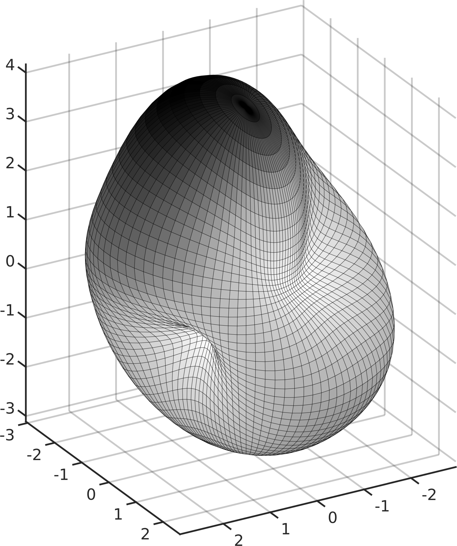
(a) Surface Plot of $(3+f(y))\cdot y$

(b) Decay of the $L_{\infty}$ error (23) of the MLS approximation of $f$ w.r.t. different ansatz spaces and bases as the fill distance goes to zero.

An easy and effective way to obtain a stable approximation process is to replace the global basis $Y_{3,2}$ of $\mathcal{H}_{L,2}({\mathbb{S}}^{2})$ by a local basis of the same space. To this end we consider the monomial basis ${\mathcal{B}}_{3,2}$ from Lemma 3.6 and utilize for $y\in{\mathbb{S}}^{2}$ an arbitrary rotation $\bm{R}_{y}\in\mathcal{SO}(3)$ that maps $y$ into the north pole, i.e. $\bm{R}_{y}y=e_{3}$ to define a local basis

$${\mathcal{B}}_{3,2}(y)\coloneqq\left\{g\circ\bm{R}_{y}\,\middle|\,g\in{\mathcal{B}}_{3,2}\right\}.$$

of the same space. The corresponding approximation error $L_{\infty}$ is depicted by the red line in Fig. 3(b) and decays all the way down to almost machine accuracy.

A similar approximation error is obtained when using the local ansatz spaces $\widetilde{{\mathcal{P}}}_{3}({\mathbb{R}}^{2},{\pi}^{-1},y)$ as introduced in Section 5. Here we consider the monomial basis (17) on the tangent space $T_{e_{3}}{\mathbb{S}}^{2}$ to the sphere at the north pole $e_{3}$ and use the rotation $\bm{R}_{y}$ and the projection $\pi\colon T_{e_{3}}{\mathbb{S}}^{2}\xrightarrow{\ \ }{\mathbb{S}}^{2}$ to derive local ansatz spaces for each $y\in{\mathbb{S}}^{2}$. The most significant difference to the previous setting is that not only the basis changes with the local point of approximation but the entire ansatz space.

References

[1]K. Atkinson and W. Han
“Spherical Harmonics and Approximations on the Unit Sphere: An Introduction” 2044, Lecture Notes in Mathematics
Springer, Heidelberg, 2012, pp. x+244
DOI: 10.1007/978-3-642-25983-8
[2]S.. Axler
“Harmonic Function Theory” 137, Springer eBook Collection Mathematics and Statistics
New York, NY: Springer, 2001
DOI: 10.1007/978-1-4757-8137-3
[3]G. Backus and F. Gilbert
“Numerical applications of a formalism for geophysical inverse problems”
In Geophys. J. R. Astron. Soc.13, 1967, pp. 247–276
[4]L. Bos and K. Salkauskas
“Moving least-squares are backus-gilbert optimal”
In J. Approx. Theory59, 1989, pp. 267–275
[5]C.. Efthimiou and C. Frye
“Spherical harmonics in p dimensions”
SingaporeHackensack, N.J: World Scientific Pub. Co, 2014
[6]G.. Fasshauer
“Meshfree approximation methods with MATLAB” 6, Interdisciplinary mathematical sciences
New Jersey: World Scientific, 2008
[7]F. Filbir and W. Themistoclakis
“Polynomial approximation on the sphere using scattered data”
In Math. Nachr.281, 2008, pp. 650–668
[8]F. Filbir, R. Hielscher, T. Jahn and T. Ullrich
“Marcinkiewicz–Zygmund inequalities for scattered and random data on the -sphere”, 2023
arXiv:2303.00045 [math.NA]
[9]M. Golitschek and W.. Light
“Interpolation by Polynomials and Radial Basis Functions on Spheres”
In Constructive Approximation17.1, 2001, pp. 1–18
DOI: 10.1007/s003650010028
[10]K. Hesse and Q.. Gia
“Local radial basis function approximation on the sphere”
In Bulletin of the Australian Mathematical Society77, 2008, pp. 197–224
DOI: 10.1017/S0004972708000087
[11] K. Jetter, J. Stöckler and J. D. Ward
“Error estimates for scattered data interpolation on spheres”
In Math. Comput.68, 1999, pp. 733–747
[12]J. Keiner and D. Potts
“Fast evaluation of quadrature formulae on the sphere”
In Math. Comput.77, 2008, pp. 397–419
DOI: 10.1090/S0025-5718-07-02029-7
[13]S. Kunis
“A note on stability results for scattered data interpolation on Euclidean spheres”
In Adv. Comput. Math.30, 2009, pp. 303–314
[14]D. Levin
“The approximation power of moving least-squares”
In Mathematics of Computation67.224, 1998, pp. 1517–1531
[15]S. Mildenberger and M. Quellmalz
“A double Fourier sphere method for d-dimensional manifolds”
In Sampling Theory, Signal Processing, and Data Analysis21, 2023
DOI: 10.1007/s43670-023-00064-8
[16]S. Mildenberger and M. Quellmalz
“Approximation Properties of the Double Fourier Sphere Method”
In Journal of Fourier Analysis and Applications28, 2022
DOI: 10.1007/s00041-022-09928-4
[17]C. Müller
“Spherical Harmonics” 17, Springer eBook Collection Mathematics and Statistics
Berlin, Heidelberg: Springer Berlin Heidelberg, 1966
DOI: 10.1007/BFb0094775
[18]D. Potts, G. Steidl and M. Tasche
“Fast and stable algorithms for discrete spherical Fourier transform”
In Linear Algebra and its ApplicationsNew York, NY: American Elsevier Publ., 1998, pp. 433–450
URL: https://madoc.bib.uni-mannheim.de/13625/
[19]D. Shepard
“A two-dimensional interpolation function for irregularly spaced points”
In Proc. 1968 Assoc. Comput. Machinery National Conference, 1968, pp. 517–524
[20]Barak Sober, Yariv Aizenbud and David Levin
“Approximation of functions over manifolds: A Moving Least-Squares approach”
In Journal of Computational and Applied Mathematics383, 2021, pp. 113140
DOI: https://doi.org/10.1016/j.cam.2020.113140
[21]D.. Varshalovich, A.. Moskalev and V.. Khersonskii
“Quantum Theory of Angular Momentum”
Singapore: World Scientific, 1988
[22]H. Wendland
“Local polynomial reproduction and moving least squares approximation”
In IMA Journal of Numerical Analysis21.1, 2001, pp. 285–300
DOI: 10.1093/imanum/21.1.285
[23]H. Wendland