Visually Grounded Continual Language Learning with Selective Specialization

Abstract

A desirable trait of an artificial agent acting in the visual world is to continually learn a sequence of language-informed tasks while striking a balance between sufficiently specializing in each task and building a generalized knowledge for transfer. Selective specialization, i.e., a careful selection of model components to specialize in each task, is a strategy to provide control over this trade-off. However, the design of selection strategies requires insights on the role of each model component in learning rather specialized or generalizable representations, which poses a gap in current research. Thus, our aim with this work is to provide an extensive analysis of selection strategies for visually grounded continual language learning. Due to the lack of suitable benchmarks for this purpose, we introduce two novel diagnostic datasets that provide enough control and flexibility for a thorough model analysis. We assess various heuristics for module specialization strategies as well as quantifiable measures for two different types of model architectures. Finally, we design conceptually simple approaches based on our analysis that outperform common continual learning baselines. Our results demonstrate the need for further efforts towards better aligning continual learning algorithms with the learning behaviors of individual model parts.

1 Introduction

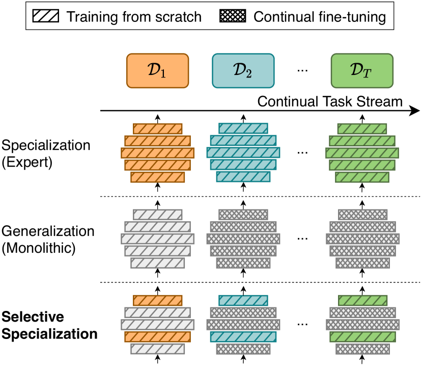
Figure 1: The specialization-generalization trade-off in a continual learning setting. Expert solutions train a copy of the network for each new task, while monolithic networks make unrestricted updates to all parameters. In this paper, we focus on selective specialization to strike a balance between full specialization and generalization.

Grounding language in visual perception is a crucial step towards agents that effectively understand and interact with the physical world (Bisk et al., 2020). In a realistic setting, such an agent would require the ability to continuously integrate novel experience and skills with existing knowledge in an open-ended process, a challenge commonly known as Continual Learning (CL) (Chen and Liu, 2018; Parisi et al., 2019; Wang et al., 2023).

Ideally, the underlying neural model of an agent would sufficiently solve each isolated task (i.e., specialization) while harnessing the shared structure and subproblems underlying all tasks to create generalizable representations for knowledge transfer (i.e., generalization). A strategy to provide control over this trade-off is to introduce task-specific parameters to a carefully selected subset of model components (i.e., selective specialization), as can be seen in Fig. 1.

Understanding which model components (here referred to as modules) are suited for task-specialization requires insights on their role in solving each task, which prior works on continual Vision-Language (VL) grounding fail to explain. At the same time, there is a lack of suitable benchmarks that allow for a fine-grained model analysis, as existing CL scenarios for language grounding based on synthetic images are too simplistic concerning the CL problem (e.g., only one distributional shift) (Greco et al., 2019) or the VL grounding problem (e.g., single-object, trivial language) (Skantze and Willemsen, 2022), while those based on real-world images (Srinivasan et al., 2022; Jin et al., 2020) may encourage models to take shortcuts in the vision-language reasoning process, which leaves the generalizability of statements derived from any model analysis questionable. To this end, we introduce the LIfelong LAnguage Compositions (LILAC) benchmark suite that comprises two diagnostic VL datasets that allow for investigating the continual learning behavior of the models with a high degree of control and flexibility while being challenging enough to require object localization, spatial reasoning, concept learning, and language grounding capabilities of the continual learner.

Based on the two proposed LILAC benchmarks, we conduct a fine-grained analysis of two different vision-language model architectures in this work that comprises the following steps: (i) We analyze whether selective specialization generally benefits from dividing the learning process into the two intermittent stages of task adaptation, where only the specialized parameters are being updated, and knowledge consolidation, where only the shared parameters are updated with respect to the task-specific learned representations. (ii) We derive and evaluate heuristics from prior literature about introducing task-specific parameters with respect to different layer depths and specific VL network modules. (iii) We assess the suitability of parameter importance measures from pruning research as indicators of the efficacy of module selection strategies.

We conclude our work by demonstrating the superior performance of module selection strategies found in our analysis, when trained under the adaptation-consolidation (A&C) procedure as described above, over common CL baselines. Thus, we summarize the contributions made in our work as follows:

1. We propose two novel datasets for visually grounded continual language learning whose problem spaces have a well-defined shared structure, thus inherently promoting a careful selection of specialized modules (cf. Sec. 3).

2. We provide a thorough analysis of the efficacy of different selective specialization strategies for two representative vision-language architectures (cf. Sec. 4.2.1–Sec. 4.2.3).

3. We show that carefully balancing the trade-off between generalization and specialization via selective specialization helps us design simple approaches that outperform CL baselines (cf. Sec. 4.2.4), ultimately demonstrating the importance of aligning CL methods with the learning behavior of individual model components.

2 Background

2.1 Continual Learning Setting

An overview of the learning setting is provided in Fig. 2. We consider a VL model composed of a language encoder $g(\cdot)$, a visual feature extractor $h(\cdot)$, a VL fusion network $f_{\theta}(\cdot)$, and a decoder $d(\cdot)$. We initialize the model at time $t_{\text{init}}$ and freeze $g$, $h$, and $d$ afterwards. After initialization, the model learns an ordered sequence of tasks from their training sets $\mathcal{D}_{t}$ for $t\in\{1,2,\dots,T\}$ and updates VL fusion parameters $\theta$ to perform well on the test sets. We assume access to the task identity of every model input during training and testing. Each data point in $\mathcal{D}_{t}$ is composed of visual observations and input instructions $(\mathbf{l}_{t},\mathbf{o}_{t},(\mathbf{o}_{t}^{+},\mathbf{o}_{t}^{-}))$ where $\mathbf{o}_{t}^{+}$ and $\mathbf{o}_{t}^{-}$ denote the visual scenes corresponding to a correct and a wrong execution of the instruction $\mathbf{l}_{t}$ upon observing $\mathbf{o}_{t}$, respectively. This setting is an extension of Natural Language Inference (Bowman et al., 2015) towards visual language grounding that can be approached using contrastive learning (Li et al., 2023), where we consider $(\mathbf{o}_{t},\mathbf{l}_{t})$ to be an image-text premise and $\mathbf{o}_{t}^{+},\mathbf{o}_{t}^{-}$ to be visual hypotheses.

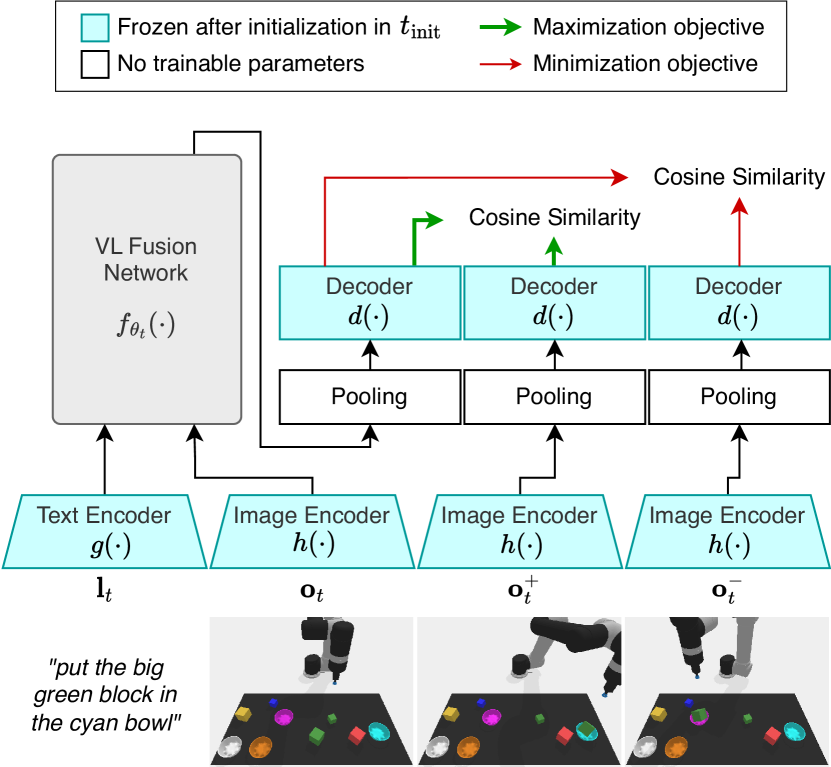
Figure 2: Overview of the model training on a LILAC-3D example. Each of the $L$ vision-language fusion layers (gray box) contains modules $m$ that are candidates for specialization.

2.2 The Specialization-Generalization Trade-off

Let $\theta_{t}$ denote the set of parameters that contains a subset of parameters specific to task $t$. Then we can express the learning objective as finding parameter values $\theta_{1},\dotsc,\theta_{T}$ for network $f_{\theta_{t}}$ that maximize the average accuracy across all test sets. From this objective arises a parameter-sharing trade-off between specialization and generalization that can be addressed by different design choices for $f$ (Ostapenko et al., 2021).

One approach is to use a monolithic network with parameters to be fully shared across tasks such that $\theta=\theta_{t}\ \forall\ t\in\{1,\dotsc,T\}$ (Kirkpatrick et al., 2017; Chaudhry et al., 2019b), which facilitates knowledge transfer between tasks at the cost of forgetting. The opposite approach is to train task-specific expert solutions (Aljundi et al., 2017; Rusu et al., 2016) such that $\theta_{i}\cap\theta_{j}=\emptyset$ for $i,j\in\{1,\dotsc,T\}$ with $i\neq j$, which alleviates forgetting at high memory most and impeded transfer. van de Ven and Tolias (2019) propose to balance this trade-off by learning task-specific “multi-headed” output layers. However, this approach assumes a uniform feature space and does not work for VL fusion networks that are trained continually.

Inspired by works on modular continual learning (Ostapenko et al., 2021; Mendez and Eaton, 2021; Mendez et al., 2022), we consider $f$ as a set $\mathcal{M}$ of modules, where a module $m$ in this context can be any kind of self-contained parametric function in $f$ (e.g., a convolutional layer or a batch normalization layer). Our aim is to find a strategy for selecting a subset $\mathcal{S}\subset\mathcal{M}$ of modules that is task-specific and parameterized by $\theta_{t}^{\mathcal{S}}$ for $t\in\{1,\dotsc,T\}$, while keeping the remaining modules shared across tasks, thus parameterized by $\theta^{\mathcal{M}\backslash\mathcal{S}}$, yielding $\theta_{t}=\{\theta^{\mathcal{S}}_{t},\theta^{\mathcal{M}\backslash\mathcal{S}}\}$. Notably, $\mathcal{S}=\emptyset$ for a monolithic (or fully shared) network and $\mathcal{S}=\mathcal{M}$ for the expert solutions.

2.3 Intermittent Adaptation and Consolidation (A&C)

We apply a simplified version of the lifelong compositional learning scheme introduced in Mendez and Eaton (2021) that is inspired by Piaget’s theories on intellectual development (Piaget, 1976) and has been successfully applied in CL of neural architectures with specialized modules: Instead of updating $\theta_{t}$ jointly upon learning task $t$, we repeatedly alternate between multiple adaptation steps (here, epochs) to update the task-specific parameters $\theta^{\mathcal{S}}_{t}$ (assimilation, fast learning) and a single consolidation step that updates the shared parameters $\theta^{\mathcal{M}\backslash\mathcal{S}}$ (accommodation, slow learning). We show in Sec. 4.2.1 that the adaptation-consolidation (A&C) learning scheme can consistently improve performance over joint optimization of $\theta_{t}$. The algorithm pseudocode can be found in Sec. A.5.

3 LILAC Datasets

In what follows, we propose two benchmark datasets that explicitly model the compositional nature of a problem, thus maintaining a high degree of overlap across tasks. This should encourage the models to use as few task-specific parameters as possible and facilitate the exploration of a reasonable selection strategy for specialized modules. During training, the model receives as input three images representing objects in a simulated environment, along with a templated language instruction. Examples of the two proposed datasets can be found in Fig. 2 and Fig. 3.

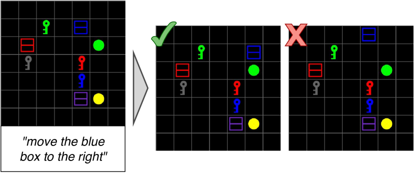
Figure 3: Example of the LILAC-2D dataset. Based on the instruction and the visual premise, a model learns to separate the two visual hypotheses (true target image, false target image) corresponding to a right and a wrong understanding of the instruction, respectively.

LILAC-2D tasks.

This dataset is based on the minigrid (Chevalier-Boisvert et al., 2018) environments. For each example, three to nine objects are randomly placed in a $7\times 7$ grid. Each instruction describes a desired interaction with a designated target object and takes the form of “move the <color> <object> <direction>”, where we choose from a set of six colors, three object types, and four directions. All three subproblems described by the instruction can be orthogonally combined, yielding $6\times 3\times 4=72$ distinct instructions. False target images are generated by randomly choosing one of the three subproblems to be wrongly solved, e.g., a blue key is moved down, although a green key was supposed to be moved down. The LILAC-2D dataset comprises 500 train, 100 validation, and 100 test samples per instruction, yielding a total of 36,000 train and 7,200 validation and test samples, respectively. For the continual learning stream, we construct $T=10$ tasks comprising training samples of six different instructions each and keep samples from the remaining 12 instructions for model initialization at time $t_{\text{init}}$.

LILAC-3D tasks.

To further narrow the gap to real 3D images while maintaining a high degree of control and flexibility for model analysis, we additionally propose LILAC-3D, a dataset with increased spatial complexity and distracting information. It is based on the simulated Ravens (Zeng et al., 2021) benchmark and its extension towards language instructions (Shridhar et al., 2022). Images show a tabletop scenario, where between five and eight blocks and between three and four bowls are randomly placed within the range of a robot arm. Instructions describe a pick-and-place operation with a target block and a target bowl and take the form of “put the <size> <color1> block in the <color2> bowl”, where we choose from a set of two different sizes, six block colors, and six bowl colors, thus yielding a total of $2\times 6\times 6=72$ distinct instructions. The sets of colors for blocks and bowls are fully disjoint to allow the objects to be clearly distinguished from one another. False target images are designed in a way that either the wrong block and the right bowl or the right block and the wrong bowl are chosen for interaction. The dataset statistics as well as the continual stream design are similar to those of the LILAC-2D dataset.

4 Evaluations

4.1 Experimental Setup

Model architectures.

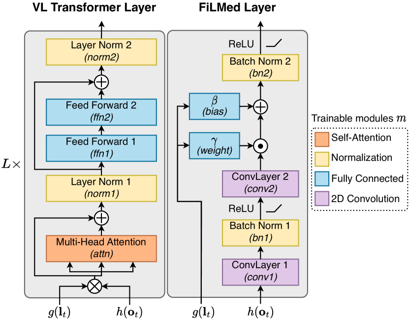
Figure 4: The two VL fusion networks $f_{\theta_{t}}(\cdot)$ used in our experiments consist of $L$ consecutive VL transformer or FiLMed layers. Each network receives as input the encoded language input and vision input to produce a joint representation $f_{\theta_{t}}(g(\mathbf{l}_{t}),h(\mathbf{o}_{t}))$. Each colored box is a module $m$ and one or multiple modules can be part of a selection strategy $\mathcal{S}$.

We conduct experiments with a transformer encoder (Vaswani et al., 2017) and a feature-wise linear modulation (FiLM) network (Perez et al., 2018) as our VL fusion networks $f_{\theta_{t}}(\cdot)$, which are both well established in research on visual language grounding both in supervised and imitation learning settings (cf. Tan and Bansal, 2019; Chen et al., 2020; Panos et al., 2023; Hui et al., 2020; Lee et al., 2022). An overview of the two VL fusion networks can be found in Fig. 4, where we also indicate the modules that we consider for selection strategies in the experiments. We use the first block of a ResNet-18 (He et al., 2016) as image encoder $h(\cdot)$. For the VL transformer, $g(\cdot)$ is the concatenation of word embeddings of the input instruction, whereas for the FiLMed network, $g(\cdot)$ is a sequence encoding by a single-layer Gated Recurrent Unit (GRU) (Cho et al., 2014). The projection decoder $d(\cdot)$ is a linear fully-connected layer. The VL fusion is followed by a max-pooling operation for FiLM and a mean-pooling operation for the transformer. All model configurations were found based on extensive hyperparameter tuning to achieve maximum performance on each validation set in the i.i.d. training setting and are described in detail in Appendix A.

Baselines.

We compare to the following baselines: Sequential fine-tuning (SFT) performs unrestricted updates on a monolithic architecture with all module parameters shared across tasks and is usually considered as a lower bound for CL model performance. Experience replay (ER) (Chaudhry et al., 2019b) is an extension to SFT which stores samples in a fixed-size buffer via reservoir sampling, from which samples are drawn for rehearsal. Elastic Weight Consolidation (EWC) (Kirkpatrick et al., 2017) is another extension to SFT that regularizes parameter updates depending on their relative importance. For our experiments, we use the Online EWC version (Schwarz et al., 2018) that does not require storing a separate approximation of the Fisher information matrix per task. Considering a potential upper bound for model performance, multi-task training (MTL) optimizes a monolithic architecture on all tasks in the i.i.d. training setting and independent experts (Expert) train a randomly initialized set of modules separately for each task.

Evaluation metrics.

We report the average accuracy across all tasks under a choice of parameters $\theta$ as $\text{ACC}^{(\theta)}$ (or, $\text{ACC}^{(\theta_{1:T})}$ for the set of all task-specific parameters $\theta_{1:T}=\{\theta_{1},\dots,\theta_{T}\}$). Furthermore, we measure the accuracy gain under a specialization strategy $\mathcal{S}$ compared with using a monolithic network as

$$\Delta\text{ACC}(\mathcal{S})=\text{ACC}^{(\theta_{1:T})}-\text{ACC}^{(\theta)},$$ (1)

where $\theta_{1:T}=\{\theta^{\mathcal{S}}_{1:T},\theta^{\mathcal{M}\backslash\mathcal{S}}\}$. Both $\text{ACC}^{(\theta_{1:T})}$ and $\Delta\text{ACC}(\mathcal{S})$ are measured after training on the last task $T$.

4.2 Results

In what follows, we first examine whether the A&C learning scheme is useful for training with a module selection strategy $\mathcal{S}$ (cf. Sec. 2.2), such that we can use A&C throughout our experiments (Sec. 4.2.1). Next, we analyze different selection strategies and compare the results with findings from prior literature (Sec. 4.2.2). We then assess whether the efficacy of selection strategies can be quantified using importance scores from pruning research (Sec. 4.2.3). Finally, we compare several selection strategies with CL baselines (Sec. 4.2.4). Each experiment is run ten times with different random seeds that affect parameter initialization and task order in the continual stream.

4.2.1 Does the A&C learning scheme benefit training with a module selection strategy?

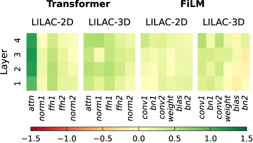
Figure 5: Difference between accuracy gains from isolating each module between A&C (cf. Alg. 1) and joint training of all shared and task-specific modules. Green values indicate the superiority of A&C over joint training.

To assess the effectiveness of the A&C learning scheme, we measure the difference in accuracy gain under the selection strategy $\mathcal{S}=\{m\}$ for each module $m\in\mathcal{M}$, as shown in Fig. 5. Overall, we observe a positive effect of introducing A&C for the majority of specialized FiLM modules and even consistently across all VL transformer modules. This indicates that despite being updated less frequently, the shared network modules learn the subproblem underlying all tasks sufficiently well while being less prone to forgetting.

4.2.2 Does the performance of different module selection strategies align with insights about general model behavior from prior literature?

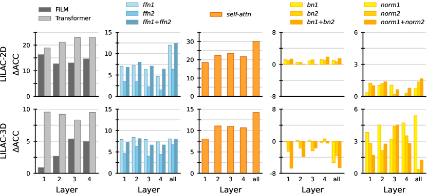
Figure 6: Evaluation of different selection strategies $\mathcal{S}$ trained with A&C for specialization. 1st column: Layer-depth analysis. 2nd+3rd column: Transformer feed-forward and multi-head attention modules. 4th+5th column: Normalization scaling factors.

Specialization at different layer depths.

To analyze the effect of isolating task parameters at different layer depths for specialization, we construct one model for each of the transformer and FiLMed layers to be specialized, respectively. The results can be found in the first column of Fig. 6.

For the VL transformer, we observe that specialization of late layers yields a higher accuracy gain than specialization of early layers. This indicates that parameters of early transformer layers benefit from being shared across tasks, as such layers learn transferable representations that should be slowly learned via infrequent updates. Such findings confirm prior research on transformers for natural language processing (Hao et al., 2019; Tenney et al., 2019) claiming that late layers capture most local syntactic phenomena, while early layers capture more general semantics.

In their analysis of FiLMed networks, Perez et al. (2018) claim that early layers perform low-level reasoning, such as querying attributes of an object, while late layers perform high-level reasoning, such as comparing two objects. As solving the LILAC-2D tasks requires the model to identify and interact with a single object, whereas for solving the LILAC-3D tasks, two objects would have to be identified and put into a shared context, we hypothesize that specialization on LILAC-2D tasks happens early and specialization on the LILAC-3D tasks happens late in the FiLMed network. As shown in the first column of Fig. 6, introducing task specialization to the first layer yields the highest accuracy gain for LILAC-2D, while the highest accuracy gain for LILAC-2D can be achieved by introducing specialized parameters to the penultimate or the last layer, which confirms our hypothesis.

Transformer feed-forward and self-attention blocks.

Geva et al. (2021) consider the outputs of the feed-forward networks to be a composition of their key-value memories and discover that such layers learn some semantic patterns, especially in early layers. Consequently, such layers can be suitable candidates for specialization during CL. The results of our experiments can be found in the second column of Fig. 6. We make two key observations, which are roughly consistent across datasets: First, isolating the first transformer feed-forward layer alone (ffn1) is as effective as isolating the entire feed-forward block (ffn1+ffn2). Second, a selective specialization of this layer improves performance most if applied in the early layers (particularly, isolation at the second transformer encoder layer yields the best performance throughout). These observations show that, when chosen carefully, selection strategies can achieve high effectiveness with only a small amount of specialized parameters.

In a recent work on parameter-efficient transfer-learning methods, Smith et al. (2023) show the efficacy of adapting self-attention blocks in a vision transformer to downstream image classification tasks while keeping the remaining transformer parameters frozen. To assess whether their findings can be transferred to our CL setting, we conduct experiments with specialized self-attention modules and report our results in the third column of Fig. 6. We observe a substantial increase in accuracy, especially for specialization in intermediate transformer layers, albeit the greatest increase ($\sim$30% on LILAC-2D, $\sim$14% on LILAC-3D) is achieved by specializing self-attention parameters across all layers. Although it is worth noting that self-attention modules account for about 73% of the parameters in each transformer layer, the results indicate a clear benefit from including self-attention parameters in specialization strategies.

Normalization scaling factors.

Bilen and Vedaldi (2017) argue that specialized instance, layer, or batch normalization scaling factors can reduce task-specific biases, allowing them to intercept distributional shifts at low additional memory cost. However, as can be seen in the penultimate column of Fig. 6, specializing batch normalization parameters of the FiLMed network hardly improves (LILAC-2D) or even degrades (LILAC-3D) performance compared with fully shared batch normalization parameters. Nevertheless, introducing task-specific layer normalization parameters in the VL transformer can slightly improve accuracy on the LILAC-2D tasks and achieves a performance gain of more than 5% on the LILAC-3D tasks. We additionally find that specializing layer normalization parameters that follow the multihead-attention operation (norm1) is generally more effective than specializing those that follow the feed-forward block (norm2), and even outperforms specializing both (norm1+norm2) on the LILAC-3D dataset.

4.2.3 Can we find quantifiable measures for the effectiveness of module selection strategies?

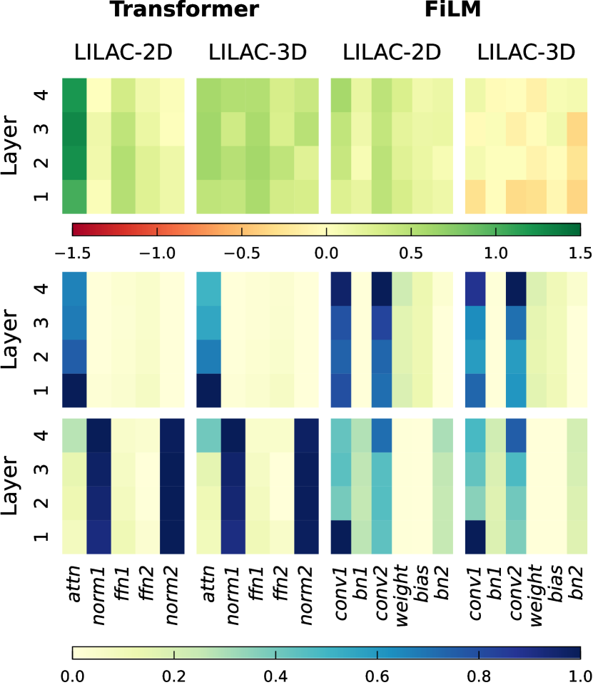
Figure 7: 1st row: Accuracy gain of each specialized module $m\in\mathcal{M}$ over fine-tuning a monolithic network. Each field represents an experiment with $\mathcal{S}=\{m\}$. 2nd row: Normalized gradient-based importance score $\text{IS}_{\text{grad}}(m)$. 3rd row: Normalized activation-based importance score $\text{IS}_{\text{act}}(m)$.

Quantifying the importance of neural connections to construct specialized weight masks is common practice in neural pruning research for CL (Molchanov et al., 2019). We aim to evaluate whether such importance scores can not only measure the suitability of specialization for single parameters but also for entire network modules. Therefore, we will compare two commonly used types of measurements for calculating the importance score (IS) of each module in the network: Gradient-based ($\text{IS}_{\text{grad}}$) and activation-based ($\text{IS}_{\text{act}}$) (cf. Wang et al., 2022; Gurbuz and Dovrolis, 2022; Jung et al., 2020). Let $\theta^{m}$ denote the parameters of network module $m$ during training and let $\theta^{m}_{t}$ denote the parameters of the $m$-th module after training on the $t$-th task.

The gradient-based importance score $\text{IS}_{\text{grad}}(m)$ of a module is computed as the sum of the $L_{1}$-norm of each parameter $w$ of $m$ and the accumulated absolute gradients arriving at $w$ during training on each task:

$$\text{IS}_{\text{grad}}(m):=\alpha\sum_{t=1}^{T}\sum_{w\in\theta_{m}}|w|+\frac{1}{2}\left|\frac{\partial\mathcal{L}(\mathcal{D}_{t};\theta)}{\partial w}\right|,$$ (2)

where the constant $\alpha=1/(T\cdot\text{log}(|\theta^{m}|))$ is used for averaging across all tasks and normalizing by the magnitude of the parameter count of $m$.

The activation-based importance score $\text{IS}_{\text{act}}(m)$ is computed as the total activation at module $m$ with the same normalization constant $\alpha$ as used above:

$$\text{IS}_{\text{act}}(m):=\alpha\sum_{t=1}^{T}\sum_{(\mathbf{l}_{t},\mathbf{o}_{t})\in\mathcal{D}_{t}}\left|f_{\theta^{m}_{t}}\left(g(\mathbf{l}_{t}),h(\mathbf{o}_{t})\right)\right|$$ (3)

We calculate the Pearson coefficient (Pearson, 1895) between the importance scores $\text{IS}_{\text{grad}}(m)$ and $\text{IS}_{\text{act}}(m)$ of each network module $m\in\mathcal{M}$ (cf. Fig. 7, second and third row) and the relative accuracy gain yielded from isolating this module for task specialization ($\mathcal{S}=\{m\}$) (cf. Fig. 7, top row).

The Pearson values for the gradient-based importance score (FiLM/Transformer) indicate a strong positive correlation for the LILAC-2D tasks ($0.91$/$0.90$) and a weak positive correlation for the LILAC-3D tasks ($0.09$/$0.40$), respectively. Conversely, there is no conclusive evidence from the activation-based importance score (2D: $0.48$/$-0.53$, 3D: $-0.09$/$-0.32$). Our results suggest that the magnitude of the gradients on the parameters of a module is a better indicator of the performance gain from specializing the whole module than the activation of the module during training. As shown in Fig. 7 (second row), the 2D convolutions in the last FiLMed layer and the attention modules in the VL transformer have high importance and thus seem to be particularly suited for specialization.

4.2.4 How does the performance of different specialization strategies compare against CL baselines?

Based on the analyses conducted in Sec. 4.2.2 and Sec. 4.2.3, our aim is to determine whether selective task specialization can outperform CL baselines for the proposed LILAC datasets. Given that all possible selection strategies form a power set that grows exponentially with the number of modules in a network, we choose the following strategies for baseline comparison: In line with the findings on specialization at different layer depths, we compare with specialization of the first layer ($\mathcal{S}_{\text{first-layer}}$) and last layer ($\mathcal{S}_{\text{last-layer}}$) for transformer and FiLMed blocks, respectively. As we found the selection of the first feed-forward network in a transformer block to be particularly effective, we further compare with the specialization of such layer across all blocks ($\mathcal{S}_{\text{all-ffn1}}$). Finally, we add the two selection strategies of specializing self-attention modules in the transformer encoder ($\mathcal{S}_{\text{all-attn}}$) and the convolutions in the last FiLMed layer ($\mathcal{S}_{\text{conv-last-layer}}$) for comparison, as the corresponding modules yield the highest $\text{IS}_{\text{grad}}$ scores. The results are reported in Tab. 1.

Table 1: ACC scores of baselines for the proposed datasets and model architectures. All selective specialization baselines are trained with A&C learning. Results from other selection strategies as well as forgetting and forward transfer measures can be found in Appendix B.

	Transformer		FiLM
Baseline	2D	3D	2D	3D
Expert	$85.9$	$88.4$	$76.5$	$78.7$
MTL	$88.3$	$95.4$	$87.1$	$80.1$
SFT	$51.1$	$67.0$	$52.1$	$63.2$
ER	$52.4$	$77.7$	$53.1$	$66.9$
EWC	$55.5$	$79.0$	$56.1$	$69.0$
$\mathcal{S}_{\text{first-layer}}$	$70.0$	$76.5$	$68.4$	$64.2$
$\mathcal{S}_{\text{last-layer}}$	$74.2$	$76.5$	$66.8$	$68.2$
$\mathcal{S}_{\text{all-ffn1}}$	$63.1$	$75.0$	-	-
$\mathcal{S}_{\text{conv-last-layer}}$	-	-	$59.4$	$62.5$
$\mathcal{S}_{\text{all-attn}}$	$81.2$	$81.2$	-	-
$\mathcal{S}_{\text{all-attn}}$ + ER	$85.7$	$88.5$	-	-
$\mathcal{S}_{\text{all-attn}}$ + EWC	$87.1$	$87.9$	-	-

Multiple selection strategies exhibit superior performance compared to CL baselines on LILAC-2D tasks. However, the sole strategy that surpasses all baselines on LILAC-3D is the specialization of attention across all layers. A possible explanation is that learning LILAC-2D tasks is generally more brittle and subject to forgetting than learning LILAC-3D tasks, as can be seen in Fig. 8. Thus, a reasonable module specialization strategy significantly increases a model’s robustness to forgetting.

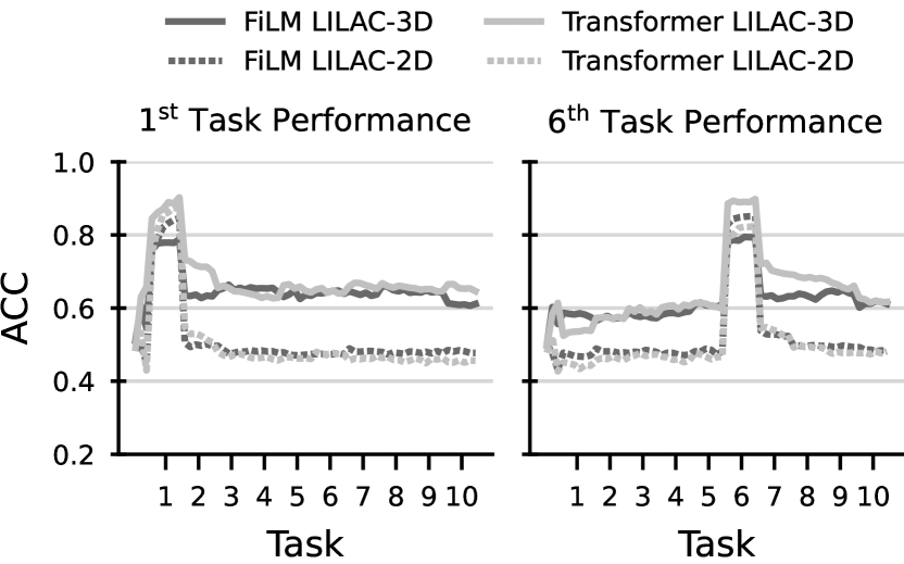
Figure 8: Accuracy of the SFT baseline on the first and the sixth task during training. LILAC-2D tasks are almost completely unlearned during training of the following tasks. Conversely, after training on LILAC-3D tasks, model performance has a slower decrease and tasks are not fully unlearned despite a lack of means to prevent forgetting.

An advantage of selective specialization is that it can be orthogonally combined with CL methods following the paradigms of replay or regularization. We find in our experiments that combining the most successful specialization strategy $\mathcal{S}_{\text{all-attn}}$ with ER or EWC by performing rehearsal or regularization during the consolidation phase of A&C learning reaches an accuracy close to the network of experts and even outperforms it by a $1.2\%$ margin ($\mathcal{S}_{\text{all-attn}}$ + EWC on LILAC-2D). Such results indicate that a combination of selective specialization with other CL methods is not only robust to forgetting but actually promotes transfer between shared modules, thus successfully striking the balance between specialization and generalization.

5 Related Work

Continual learning.

In a CL scenario, an agent is exposed to a sequence of tasks with the objective of learning to solve the currently seen task while maintaining high performance on previous tasks. Approaches to CL can be broadly categorized into regularization (Kirkpatrick et al., 2017; Zenke et al., 2017; Li and Hoiem, 2018; Aljundi et al., 2018) that restrict parameter updates to bound plasticity, (pseudo-)rehearsal (Rebuffi et al., 2017; Chaudhry et al., 2019a; Buzzega et al., 2021), where data that are either retrieved from a memory buffer or synthetically generated from previous distributions are periodically replayed to the model, and dynamic architectures (Rusu et al., 2016; Yoon et al., 2018), where models are gradually expanded in response to distributional shifts.

A few works explore the intersection of continual learning and visually grounded language learning with diagnostic (Skantze and Willemsen, 2022; Greco et al., 2019) and real-world (Srinivasan et al., 2022; Jin et al., 2020) datasets. All works conclude that common CL baselines struggle with striking a balance between forgetting and cross-task knowledge transfer, yet do not provide any insights on how this struggle is connected with the learning behaviors of the architecture used.

Introducing task-specific parameters.

Research on continual neural pruning assigns some model capacity to each task by iteratively pruning and retraining (sub-)networks that are specialized to each task (Mallya and Lazebnik, 2018; Geng et al., 2021; Dekhovich et al., 2023; Kang et al., 2022; Hung et al., 2019; Gurbuz and Dovrolis, 2022; Jung et al., 2020; Wang et al., 2022). However, while such methods are effective in overcoming forgetting, the evolution and learning behavior of pruned subnetworks provides little interpretability regarding the role of individual parts of the network in solving CL problems.

Another line of research is modular CL, which trains a structural combination of independent parameterized components under the common assumption that each component solves a subproblem of each given task (Mendez and Eaton, 2021; Mendez et al., 2022; Ostapenko et al., 2021; Veniat et al., 2021). Similarly to neural pruning, approaches to modular CL fail to explain which role the interplay between learnable structural configurations and shared components takes in solving the tasks. In this topic area, the analysis provided by Csordás et al. (2021) is closely related to our work, except that we analyze model behavior on the level of entire modules rather than isolated parameters.

In an effort to promote parameter-efficient transfer in CL with foundation models, recent works utilize task-specific plugins such as capsule networks (Ke et al., 2021a) or adapters (Ke et al., 2021b; Zhao et al., 2022; Ermis et al., 2022) that leverage the pretrained representations as shared structure. This line of research is parallel to ours rather than competing, as we analyze existing parts of a trainable model rather than adding additional components to pretrained networks.

6 Conclusion

Striking a balance between specialization and generalization poses a challenge for agents that learn a sequence of language-conditioned tasks grounded in a visual environment. In this work, we consider vision-language models as a composition of modules and propose two datasets that allow us to analyze and compare strategies to selectively specialize modules to continual tasks with respect to different layer depths and module types. We further establish a gradient-based importance measure that quantifies the suitability of modules for specialization. Finally, we show that the module specialization strategies found in our analysis outperforms common CL baselines when trained under a conceptually simple adaptation-consolidation learning scheme. With this work, we show the merit of designing CL methods based on a careful analysis of selective specialization. Beyond introducing specialization to existing model parts, we plan to leverage our insights for the design of parameter isolation CL methods that introduce additional parameters into a pretrained model for future work.

Limitations

Generally, we consider the results and analyses provided in this paper to be merely a cornerstone towards gaining more knowledge about model behavior during learning, an insight that can be used to better understand where in a model to introduce task-specific parameters. Nevertheless, we recognize the following limitations of our work: First, we conduct our experiments with two established vision-language architectures with just one model configuration each. More notably, the architectures we use are smaller and conceptually simpler than those used for large-scale realistic datasets on visual language grounding. Second, introducing task specialization to network modules naturally has a linear growth with the number of tasks. This can, however, be mitigated by choosing smaller modules for specialization with reasonable performance to strike a balance between parameter size and model performance.

Appendix A Experimental Settings

A.1 LILAC-2D and LILAC-3D Datasets

Examples of both datasets are provided in Fig. 2 and Fig. 3. For the LILAC-2D dataset, object colors are {blue, green, grey, purple, red, yellow}, object types are {ball, box, key}, and directions are {down, to the left, to the right, up}. For the LILAC-3D dataset, blocks have the colors {blue, green, grey, purple, red, yellow}, bowls have the colors {brown, cyan, orange, petrol, pink, white}, and block sizes are {big, small}.

A.2 Model Architectures

In the following, we describe further details about the two model architectures used in our experiments.

FiLM.

The FiLMed layer is illustrated in the left part of Fig. 4. We largely follow the architectural design of the FiLMed layers as suggested in Hui et al. (2020): Each FiLMed layer consists of a ConvBlock and the linear modulation fully-connected layers $\gamma$ (weight) and $\beta$ (bias) that condition the feature maps of the convolutional layers by scaling by the factor $\gamma$ and shifting by the value $\beta$. The ConvBlock consists of two two-dimensional convolutional layers with a kernel size of $3$, a stride of $1$, and a padding of $1$, and two batch norm layers. Features of visual observations $\mathbf{o}_{t}$, $\mathbf{o}_{t}^{+}$, and $\mathbf{o}_{t}^{-}$ are initially extracted by the first block of a ResNet-18 (this configuration yielded better performance on both datasets than using the feature extractor as proposed in Hui et al. (2020)). Subsequently, the visual features of the premise observation $\mathbf{o}_{t}$ are passed through the first convolutional layer, followed by batch normalization, rectified linear unit (ReLU) activation, and the second convolutional layer. The language instruction $\mathbf{l}_{t}$ is passed through a word embedding layer, followed by a single-layer GRU. The embedded instruction sequence is passed through the two fully connected layers $\beta$ and $\gamma$, the output of which is used to modulate the visual features from the second convolutional layer. Finally, the modulated features are passed through a second batch normalization layer and ReLU activation. After passing $L$ FiLMed blocks, the features are max-pooled across the height and width of the feature maps and finally passed through a linear projection layer. In contrast to the ‘premise’ observation $\mathbf{o}_{t}$, ResNet-18 features of the visual observations $\mathbf{o}_{t}^{+}$ and $\mathbf{o}_{t}^{-}$ are directly max-pooled and passed through the linear projection layer.

Vision-Language Transformer.

The right part of Fig. 4 provides an overview of the transformer architecture used in our experiments. Each transformer encoder layer follows the original design as proposed in Vaswani et al. (2017) and consists of a multi-head attention operation, two normalization layers, and two fully connected feed-forward layers. Similarly to the FiLM model, visual features of $\mathbf{o}_{t}$, $\mathbf{o}_{t}^{+}$, and $\mathbf{o}_{t}^{-}$ are extracted from the first block of a ResNet-18 encoder and passed through an additional linear encoder layer to match the latent dimension of the word embeddings from the input instruction $\mathbf{l}_{t}$. Word embeddings of $\mathbf{l}_{t}$ and visual features of $\mathbf{o}_{t}$ are then concatenated and fed to a multi-head attention layer, followed by a residual adding operation layer normalization. Afterwards, the latent VL features are passed through two fully connected linear layers, i.e., the feed-forward blocks of the network, which is again followed by a residual operation and layer normalization. After passing the total of $L$ transformer encoder layers, the features are mean-pooled across the height and width of the language-conditioned feature maps and fed to a linear projection layer. In the same way as with the FiLM architecture, visual features of $\mathbf{o}_{t}^{+}$ and $\mathbf{o}_{t}^{-}$ from the ResNet-18 are directly pooled and passed through the projection layer.

A.3 Hyperparameter Configuration

An overview of the design choices and selected parameters for the model architectures can be found in Tab. 2.

Table 2: Overview of the hyperparameters selected for the model architectures with respect to the two datasets. We used the Weights&Biases (https://wandb.ai/site) sweep with Bayes optimizer.

	Transformer		FiLM		Search space
	2D	3D	2D	3D
init lr	4.5e-4	2e-4	4.5e-4	2e-4	[1e-6, 1e-3]
continual lr	6e-4	7e-4	8e-4	1e-3	[1e-6, 1e-3]
batch size	128	128	128	128	-
init epochs	10	10	10	10	-
continual epochs (per $t$)	30	30	30	30	-
word embedding dim	256	256	128	128	{32, 64, 128, 256, 512}
instr embedding dim	-	-	256	256	{32, 64, 128, 256, 512}
ResNet-18 layer features	1	1	1	1	{1, 2, 3, 4}
encoder layers ($L$)	4	4	4	4	{ 1, 2, 4, 6, 8, 10, 12 }
attn heads	2	2	-	-	{ 1, 2, 4, 6, 8}
ffn dim	64	64	-	-	{32, 64, 128, 256, 512}
EWC discount	0.9	0.9	0.9	0.9	[ 0, 1 ]
EWC $\lambda$ (joint)	2,000	600	2,000	600	[1e-2, 1e14]
EWC $\lambda$ (A&C)	20,000	20,000	20,000	20,000	[1e-2, 1e14]
ER buffer size	3,000	3,000	3,000	3,000	-

A.4 Metrics and Performance Evaluation

During training, we use the InfoNCE loss (Oord et al., 2019) $\mathcal{L}_{\text{info}}$ to maximize the cosine similarity between $d(f_{\theta_{t}}(h(\mathbf{o}_{t}),g(\mathbf{l}_{t})))$ and $d(h(\mathbf{o}_{t}^{+}))$ and minimize the cosine similarity between $d(f_{\theta_{t}}(h(\mathbf{o}_{t}),g(\mathbf{l}_{t})))$ and $d(h(\mathbf{o}_{t}^{-}))$. During inference, the model predicts the target image by choosing the image representation of $d(h(\mathbf{o}_{t}^{+}))$, $d(h(\mathbf{o}_{t}^{-}))$ that has higher cosine similarity with the representation of $d(f_{\theta_{t}}(h(\mathbf{o}_{t}),g(\mathbf{l}_{t})))$, i.e. rCl 3lS_cos(d(f_θ_t(h(o_t), g(l_t))), d(h(o_t^+))
& > S_cos(d(f_θ_t(h(o_t), g(l_t)), d(h(o_t^-)))

The prediction accuracy $A_{t}$ can then be calculated as the number of samples of the $t$-th task for which Sec. A.4 holds, divided by the total number of samples from the $t$-th task, $|\mathcal{D}_{t}|$.

Accuracy, transfer, forgetting.

We provide more details on evaluation metrics and some additional results on catastrophic forgetting (CF), and forward transfer (FT). Let $A_{i,j}$ denote the test accuracy of a model on the $j$-th task after observing the last sample of the $i$-th task. We largely follow the commonly used evaluation metrics as proposed in Lopez-Paz and Ranzato (2017):

rCl 3lACC := 1T ∑_t = 1^T A_T, t,   CF := 1T ∑_t = 1^T-1 A_t, t - A_T, t
3lFT := 1T - 1 ∑_t = 2^T A_t-1, t - A_init, t, where $A_{\text{init},t}$ denotes the performance on the $t$-th task after initialization. Note that CF can be also interpreted as negative backward transfer, as it describes the influence of training on a task on previously seen tasks.

A.5 Adaptation-Consolidation Algorithm

The pseudocode of the A&C training algorithm as a modification to the lifelong compositional learning algorithm proposed by Mendez and Eaton (2021) is shown in Alg. 1. $\theta^{\mathcal{M}\backslash\mathcal{S}}$ denotes all shared parameters, whereas $\theta^{\mathcal{S}}_{t}$ are the task-specific, or isolated, parameters. We choose adaptFreq$=6$ for our experiments.

Algorithm 1 Adaptation-Consolidation (A&C)

Select modules $\mathcal{S}\subset\mathcal{M}$ for task specialization

Initialize all model parameters via joint training on $\mathcal{D}_{t_{\text{init}}}$

for $t=1..T$ do

     Freeze $\theta^{\mathcal{M}\backslash\mathcal{S}}$

     for $e=1..\texttt{adaptationEpochs}$ do

         Update $\theta^{\mathcal{S}}_{t}$ upon training on $\mathcal{D}_{t}$

         if $e$ mod adaptFreq = 0 then

              Freeze $\theta^{\mathcal{S}}_{t}$, unfreeze $\theta^{\mathcal{M}\backslash\mathcal{S}}$

              Update $\theta^{\mathcal{M}\backslash\mathcal{S}}$ upon training on $\mathcal{D}_{t}$

              Freeze $\theta^{\mathcal{M}\backslash\mathcal{S}}$, unfreeze $\theta^{\mathcal{S}}_{t}$

         end if

     end for

end for

Appendix B Additional Results

We provide some additional results on the effect of introducing task specialization to network modules in Fig. 9, Fig. 10, and Fig. 11. We provide more detailed results from our baseline comparison in Tab. 3. Finally, we provide two additional findings that might be interesting to the community:

FiLM modulation parameters.

We observe that introducing task-specific parameters to either the weight ($\gamma$) or bias $(\beta)$ separately yields the highest accuracy gain and forward transfer as well as the lowest forgetting. However, while the FiLMed model trained on the LILAC-2D tasks benefits most from weights to be specialized, the same model trained on LILAC-3D needs bias to be specialized to optimize performance metrics.

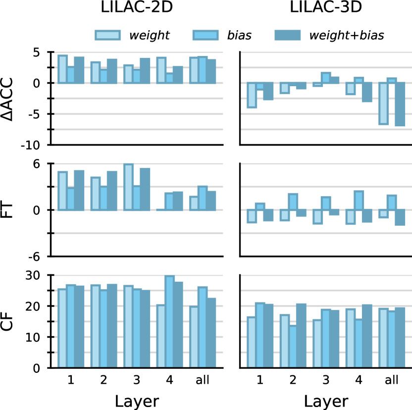
Figure 9: Analysis of specializing feature-wise linear modulation parameters in different layers. Top to bottom: 1) accuracy gain of specialization and A&C compared with monolithic SFT baseline, 2) forward transfer, and 3) forgetting.

Modules whose specialization maximized forward transfer.

While for the FiLMed network the specialization of modulation parameters (weight for LILAC-2D, bias for LILAC-3D) maximizes the forward transfer, for the VL transformer it is the feed-forward layers and the layer normalization parameters that maximize forward transfer when specialized.

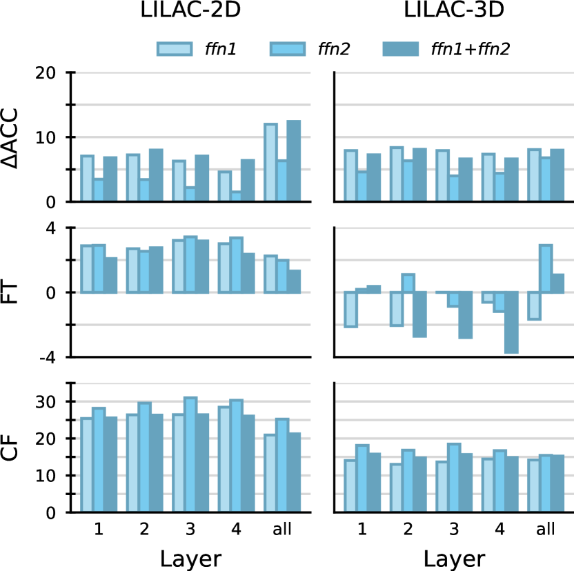
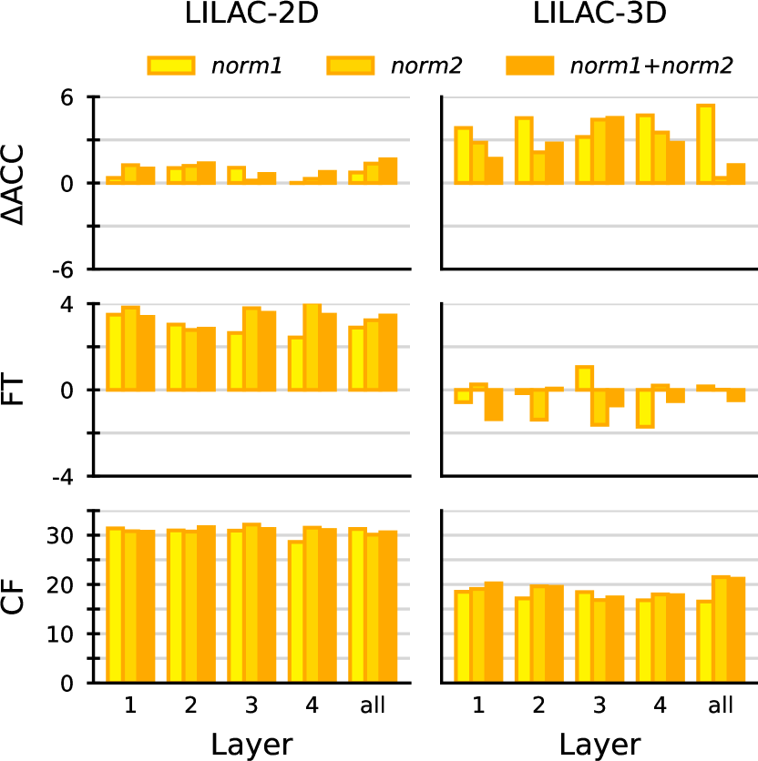
Figure 10: Analysis of specialization in different layers for feed-forward layers (top) and layer normalization parameters (bottom). Each plot shows (from top to bottom): 1) accuracy gain of specialization and A&C compared with monolithic SFT baseline, 2) forward transfer, and 3) forgetting.

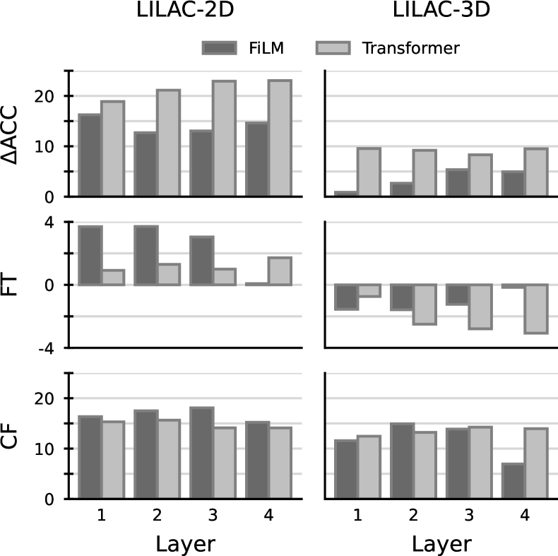
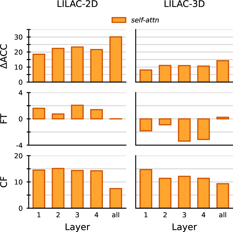
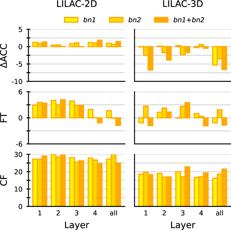
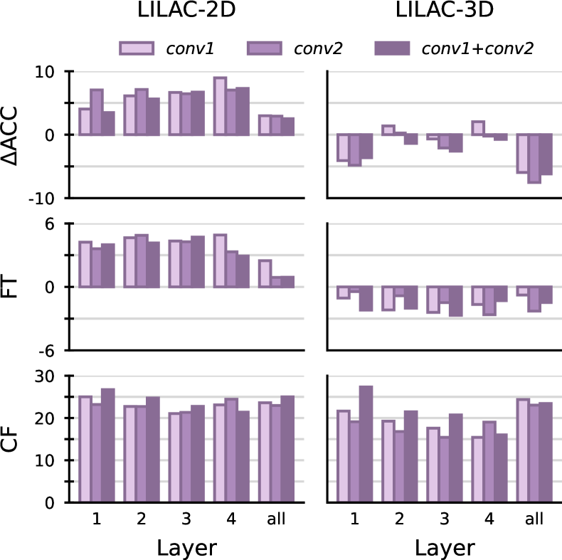
Figure 11: Analysis of specialization of layers in different depths (top left) and module specialization in different layers for self-attention (top right), batch normalization parameters (bottom left), and convolutional layers (bottom right). Each plot shows (from top to bottom): 1) accuracy gain of specialization and A&C compared with monolithic SFT baseline, 2) forward transfer, and 3) forgetting.

FiLM	LILAC-2D			LILAC-3D
	ACC	FT	CF	ACC	FT	CF
MTL	$87.1\pm 0.9\%$	-	-	$80.1\pm 1.1\%$	-	-
Expert	$76.5\pm 1.4\%$	-	-	$78.7\pm 2.7\%$	-	-
SFT	$52.1\pm 0.3\%$	$2.4\pm 0.4\%$	$35.0\pm 1.0\%$	$63.3\pm 0.8\%$	$2.5\pm 1.0\%$	$17.5\pm 1.7\%$
ER	$53.1\pm 0.3\%$	$2.7\pm 0.3\%$	$33.9\pm 0.9\%$	$66.9\pm 1.2\%$	$4.8\pm 1.4\%$	$14.6\pm 1.7\%$
EWC	$56.1\pm 0.9\%$	$2.9\pm 0.6\%$	$7.7\pm 0.9\%$	$69.0\pm 1.4\%$	$3.6\pm 0.6\%$	$10.1\pm 0.8\%$
$\mathcal{M}_{\text{first-layer}}$	$68.4\pm 0.8\%$	$3.7\pm 0.4\%$	$16.4\pm 0.5\%$	$64.2\pm 2.1\%$	$-1.6\pm 0.5\%$	$11.6\pm 0.9\%$
$\mathcal{M}_{\text{last-layer}}$	$66.8\pm 0.8\%$	$0.1\pm 0.1\%$	$15.2\pm 0.4\%$	$68.2\pm 1.8\%$	$-0.2\pm 0.3\%$	$7.0\pm 0.9\%$
$\mathcal{M}_{\text{conv-last-layer}}$	$59.4\pm 0.4\%$	$2.9\pm 0.5\%$	$21.4\pm 1.7\%$	$62.5\pm 0.9\%$	$-1.3\pm 0.6\%$	$16.0\pm 2.6\%$

Transformer	LILAC-2D			LILAC-3D
	ACC	FT	CF	ACC	FT	CF
MTL	$88.3\pm 0.3\%$	-	-	$95.4\pm 0.3\%$	-	-
Expert	$85.9\pm 0.4\%$	-	-	$88.4\pm 0.2\%$	-	-
SFT	$51.1\pm 0.2\%$	$2.5\pm 0.6\%$	$35.7\pm 0.6\%$	$67.0\pm 0.8\%$	$-2.5\pm 0.8\%$	$24.2\pm 0.6\%$
ER	$52.4\pm 0.4\%$	$2.7\pm 0.3\%$	$34.6\pm 0.5\%$	$77.7\pm 0.8\%$	$1.6\pm 0.9\%$	$12.7\pm 0.7\%$
EWC	$55.5\pm 0.7\%$	$2.2\pm 0.6\%$	$14.2\pm 0.4\%$	$79.0\pm 0.7\%$	$1.8\pm 0.9\%$	$8.9\pm 0.6\%$
$\mathcal{M}_{\text{first-layer}}$	$70.0\pm 0.4\%$	$0.9\pm 0.3\%$	$15.3\pm 0.6\%$	$76.5\pm 0.7\%$	$-0.7\pm 0.4\%$	$12.5\pm 0.7\%$
$\mathcal{M}_{\text{last-layer}}$	$74.2\pm 0.6\%$	$1.7\pm 0.3\%$	$14.1\pm 0.4\%$	$76.5\pm 1.0\%$	$-3.1\pm 0.6\%$	$14.0\pm 1.0\%$
$\mathcal{M}_{\text{all-ffn1}}$	$63.1\pm 0.5\%$	$2.3\pm 0.3\%$	$20.9\pm 0.5\%$	$75.0\pm 0.7\%$	$-1.7\pm 0.9\%$	$14.2\pm 1.0\%$
$\mathcal{M}_{\text{all-attn}}$	$81.2\pm 0.6\%$	$0.0\pm 0.3\%$	$7.5\pm 0.7\%$	$81.2\pm 0.8\%$	$0.2\pm 0.5\%$	$9.3\pm 0.9\%$
$\mathcal{M}_{\text{all-attn}}$ + ER	$85.7\pm 1.7\%$	$0.1\pm 0.2\%$	$0.8\pm 0.2\%$	$88.5\pm 0.5\%$	$-0.8\pm 0.2\%$	$0.4\pm 0.2\%$
$\mathcal{M}_{\text{all-attn}}$ + EWC	$87.1\pm 0.4\%$	$0.4\pm 0.1\%$	$0.6\pm 0.2\%$	$87.9\pm 0.5\%$	$-0.5\pm 0.3\%$	$0.6\pm 0.1\%$

Table 3: Average accuracy (ACC), forward transfer (FT), and forgetting (CF) of FiLM (top) and vision-language transformer (bottom) baselines for all datasets. Results are averaged across ten seeds. Standard error after $\pm$.

References

- Aljundi et al. (2018) Rahaf Aljundi, Francesca Babiloni, Mohamed Elhoseiny, Marcus Rohrbach, and Tinne Tuytelaars. 2018. Memory aware synapses: Learning what (not) to forget. In Proceedings of the European Conference on Computer Vision (ECCV).
- Aljundi et al. (2017) Rahaf Aljundi, Punarjay Chakravarty, and Tinne Tuytelaars. 2017. Expert Gate: Lifelong Learning With a Network of Experts. In Proceedings of the IEEE Conference on Computer Vision and Pattern Recognition (CVPR).
- Andreas et al. (2016) Jacob Andreas, Marcus Rohrbach, Trevor Darrell, and Dan Klein. 2016. Neural Module Networks. In Proceedings of the IEEE Conference on Computer Vision and Pattern Recognition, pages 39–48.
- Bilen and Vedaldi (2017) Hakan Bilen and Andrea Vedaldi. 2017. Universal representations: The missing link between faces, text, planktons, and cat breeds. ArXiv:1701.07275 [cs, stat].
- Bisk et al. (2020) Yonatan Bisk, Ari Holtzman, Jesse Thomason, Jacob Andreas, Yoshua Bengio, Joyce Chai, Mirella Lapata, Angeliki Lazaridou, Jonathan May, Aleksandr Nisnevich, Nicolas Pinto, and Joseph Turian. 2020. Experience grounds language. In Proceedings of the 2020 Conference on Empirical Methods in Natural Language Processing (EMNLP), pages 8718–8735, Online. Association for Computational Linguistics.
- Bowman et al. (2015) Samuel R. Bowman, Gabor Angeli, Christopher Potts, and Christopher D. Manning. 2015. A large annotated corpus for learning natural language inference. In Proceedings of the 2015 Conference on Empirical Methods in Natural Language Processing, pages 632–642, Lisbon, Portugal. Association for Computational Linguistics.
- Buzzega et al. (2021) Pietro Buzzega, Matteo Boschini, Angelo Porrello, and Simone Calderara. 2021. Rethinking Experience Replay: a Bag of Tricks for Continual Learning. In 2020 25th International Conference on Pattern Recognition (ICPR), pages 2180–2187.
- Chaudhry et al. (2019a) Arslan Chaudhry, Marc’Aurelio Ranzato, Marcus Rohrbach, and Mohamed Elhoseiny. 2019a. Efficient Lifelong Learning with A-GEM. In International Conference on Learning Representations.
- Chaudhry et al. (2019b) Arslan Chaudhry, Marcus Rohrbach, Mohamed Elhoseiny, Thalaiyasingam Ajanthan, Puneet K. Dokania, Philip H. S. Torr, and Marc’Aurelio Ranzato. 2019b. Continual learning with tiny episodic memories. ArXiv:1902.10486 [cs, stat].
- Chen et al. (2020) Yen-Chun Chen, Linjie Li, Licheng Yu, Ahmed El Kholy, Faisal Ahmed, Zhe Gan, Yu Cheng, and Jingjing Liu. 2020. UNITER: UNiversal Image-TExt Representation Learning. In Andrea Vedaldi, Horst Bischof, Thomas Brox, and Jan-Michael Frahm, editors, Computer Vision – ECCV 2020, volume 12375, pages 104–120. Springer International Publishing, Cham. Series Title: Lecture Notes in Computer Science.
- Chen and Liu (2018) Zhiyuan Chen and Bing Liu. 2018. Lifelong Machine Learning, Second Edition. Synthesis Lectures on Artificial Intelligence and Machine Learning, 12(3).
- Chevalier-Boisvert et al. (2018) Maxime Chevalier-Boisvert, Lucas Willems, and Suman Pal. 2018. Minimalistic gridworld environment for gymnasium.
- Cho et al. (2014) Kyunghyun Cho, Bart Van Merrienboer, Caglar Gulcehre, Dzmitry Bahdanau, Fethi Bougares, Holger Schwenk, and Yoshua Bengio. 2014. Learning Phrase Representations using RNN Encoder–Decoder for Statistical Machine Translation. In Proceedings of the 2014 Conference on Empirical Methods in Natural Language Processing (EMNLP), pages 1724–1734, Doha, Qatar. Association for Computational Linguistics.
- Csordás et al. (2021) Róbert Csordás, Sjoerd van Steenkiste, and Jürgen Schmidhuber. 2021. Are Neural Nets Modular? Inspecting Functional Modularity Through Differentiable Weight Masks. In International Conference on Learning Representations.
- Dekhovich et al. (2023) Aleksandr Dekhovich, David M.J. Tax, Marcel H.F Sluiter, and Miguel A. Bessa. 2023. Continual prune-and-select: class-incremental learning with specialized subnetworks. Applied Intelligence.
- Ermis et al. (2022) Beyza Ermis, Giovanni Zappella, Martin Wistuba, Aditya Rawal, and Cedric Archambeau. 2022. Memory Efficient Continual Learning with Transformers. In Advances in Neural Information Processing Systems, volume 35, pages 10629–10642. Curran Associates, Inc.
- Geng et al. (2021) Binzong Geng, Fajie Yuan, Qiancheng Xu, Ying Shen, Ruifeng Xu, and Min Yang. 2021. Continual learning for task-oriented dialogue system with iterative network pruning, expanding and masking. In Proceedings of the 59th Annual Meeting of the Association for Computational Linguistics and the 11th International Joint Conference on Natural Language Processing (Volume 2: Short Papers), pages 517–523, Online. Association for Computational Linguistics.
- Geva et al. (2021) Mor Geva, Roei Schuster, Jonathan Berant, and Omer Levy. 2021. Transformer Feed-Forward Layers Are Key-Value Memories. In Proceedings of the 2021 Conference on Empirical Methods in Natural Language Processing, pages 5484–5495, Online and Punta Cana, Dominican Republic. Association for Computational Linguistics.
- Greco et al. (2019) Claudio Greco, Barbara Plank, Raquel Fernández, and Raffaella Bernardi. 2019. Psycholinguistics Meets Continual Learning: Measuring Catastrophic Forgetting in Visual Question Answering. In Proceedings of the 57th Annual Meeting of the Association for Computational Linguistics, pages 3601–3605, Florence, Italy. Association for Computational Linguistics.
- Gurbuz and Dovrolis (2022) Mustafa B Gurbuz and Constantine Dovrolis. 2022. NISPA: Neuro-Inspired Stability-Plasticity Adaptation for Continual Learning in Sparse Networks. In Proceedings of the 39th International Conference on Machine Learning, volume 162 of Proceedings of Machine Learning Research, pages 8157–8174. PMLR.
- Hao et al. (2019) Yaru Hao, Li Dong, Furu Wei, and Ke Xu. 2019. Visualizing and Understanding the Effectiveness of BERT. In Proceedings of the 2019 Conference on Empirical Methods in Natural Language Processing and the 9th International Joint Conference on Natural Language Processing (EMNLP-IJCNLP), pages 4141–4150, Hong Kong, China. Association for Computational Linguistics.
- He et al. (2016) Kaiming He, Xiangyu Zhang, Shaoqing Ren, and Jian Sun. 2016. Deep Residual Learning for Image Recognition. In Proceedings of the IEEE Conference on Computer Vision and Pattern Recognition (CVPR).
- Hui et al. (2020) David Yu-Tung Hui, Maxime Chevalier-Boisvert, Dzmitry Bahdanau, and Yoshua Bengio. 2020. BabyAI 1.1. ArXiv:2007.12770 [cs].
- Hung et al. (2019) Ching-Yi Hung, Cheng-Hao Tu, Cheng-En Wu, Chien-Hung Chen, Yi-Ming Chan, and Chu-Song Chen. 2019. Compacting, Picking and Growing for Unforgetting Continual Learning. In Advances in Neural Information Processing Systems, volume 32. Curran Associates, Inc.
- Jin et al. (2020) Xisen Jin, Junyi Du, Arka Sadhu, Ram Nevatia, and Xiang Ren. 2020. Visually grounded continual learning of compositional phrases. In Proceedings of the 2020 Conference on Empirical Methods in Natural Language Processing (EMNLP), pages 2018–2029, Online. Association for Computational Linguistics.
- Jung et al. (2020) Sangwon Jung, Hongjoon Ahn, Sungmin Cha, and Taesup Moon. 2020. Continual Learning with Node-Importance based Adaptive Group Sparse Regularization. In Advances in Neural Information Processing Systems, volume 33, pages 3647–3658. Curran Associates, Inc.
- Kang et al. (2022) Haeyong Kang, Rusty John Lloyd Mina, Sultan Rizky Hikmawan Madjid, Jaehong Yoon, Mark Hasegawa-Johnson, Sung Ju Hwang, and Chang D. Yoo. 2022. Forget-free Continual Learning with Winning Subnetworks. In Proceedings of the 39th International Conference on Machine Learning, volume 162 of Proceedings of Machine Learning Research, pages 10734–10750. PMLR.
- Ke et al. (2021a) Zixuan Ke, Bing Liu, Nianzu Ma, Hu Xu, and Lei Shu. 2021a. Achieving Forgetting Prevention and Knowledge Transfer in Continual Learning. In Advances in Neural Information Processing Systems, volume 34.
- Ke et al. (2021b) Zixuan Ke, Hu Xu, and Bing Liu. 2021b. Adapting BERT for continual learning of a sequence of aspect sentiment classification tasks. In Proceedings of the 2021 Conference of the North American Chapter of the Association for Computational Linguistics: Human Language Technologies, pages 4746–4755, Online. Association for Computational Linguistics.
- Kirkpatrick et al. (2017) James Kirkpatrick, Razvan Pascanu, Neil Rabinowitz, Joel Veness, Guillaume Desjardins, Andrei A. Rusu, Kieran Milan, John Quan, Tiago Ramalho, Agnieszka Grabska-Barwinska, Demis Hassabis, Claudia Clopath, Dharshan Kumaran, and Raia Hadsell. 2017. Overcoming catastrophic forgetting in neural networks. Proceedings of the National Academy of Sciences, 114(13):3521–3526.
- Lee et al. (2022) Jae Hee Lee, Matthias Kerzel, Kyra Ahrens, Cornelius Weber, and Stefan Wermter. 2022. What is Right for Me is Not Yet Right for You: A Dataset for Grounding Relative Directions via Multi-Task Learning. In Proceedings of the Thirty-First International Joint Conference on Artificial Intelligence (IJCAI-22), pages 1039–1045. International Joint Conferences on Artificial Intelligence Organization.
- Li et al. (2023) Shu’ang Li, Xuming Hu, Li Lin, Aiwei Liu, Lijie Wen, and Philip S. Yu. 2023. A Multi-Level Supervised Contrastive Learning Framework for Low-Resource Natural Language Inference. IEEE/ACM Transactions on Audio, Speech, and Language Processing, 31:1771–1783.
- Li and Hoiem (2018) Zhizhong Li and Derek Hoiem. 2018. Learning without Forgetting. Transactions on Pattern Analysis and Machine Intelligence, 40(12).
- Lopez-Paz and Ranzato (2017) David Lopez-Paz and Marc’ Aurelio Ranzato. 2017. Gradient Episodic Memory for Continual Learning. In Advances in Neural Information Processing Systems, volume 30. Curran Associates, Inc.
- Mallya and Lazebnik (2018) Arun Mallya and Svetlana Lazebnik. 2018. PackNet: Adding Multiple Tasks to a Single Network by Iterative Pruning. In Proceedings of the IEEE Conference on Computer Vision and Pattern Recognition (CVPR).
- Mendez and Eaton (2021) Jorge A. Mendez and Eric Eaton. 2021. Lifelong Learning of Compositional Structures. In International Conference on Learning Representations.
- Mendez et al. (2022) Jorge A. Mendez, Harm van Seijen, and Eric Eaton. 2022. Modular Lifelong Reinforcement Learning via Neural Composition. In International Conference on Learning Representations.
- Molchanov et al. (2019) Pavlo Molchanov, Arun Mallya, Stephen Tyree, Iuri Frosio, and Jan Kautz. 2019. Importance Estimation for Neural Network Pruning. In Proceedings of the IEEE/CVF Conference on Computer Vision and Pattern Recognition (CVPR).
- Oord et al. (2019) Aaron van den Oord, Yazhe Li, and Oriol Vinyals. 2019. Representation Learning with Contrastive Predictive Coding. ArXiv:1807.03748 [cs, stat].
- Ostapenko et al. (2021) Oleksiy Ostapenko, Pau Rodriguez, Massimo Caccia, and Laurent Charlin. 2021. Continual Learning via Local Module Composition. In Advances in Neural Information Processing Systems, volume 34, pages 30298–30312. Curran Associates, Inc.
- Panos et al. (2023) Aristeidis Panos, Yuriko Kobe, Daniel Olmeda Reino, Rahaf Aljundi, and Richard E. Turner. 2023. First Session Adaptation: A Strong Replay-Free Baseline for Class-Incremental Learning. ArXiv:2303.13199 [cs].
- Parisi et al. (2019) German I. Parisi, Ronald Kemker, Jose L. Part, Christopher Kanan, and Stefan Wermter. 2019. Continual lifelong learning with neural networks: A review. Neural Networks, 113:54–71.
- Pearson (1895) Karl Pearson. 1895. Note on regression and inheritance in the case of two parents. Proceedings of the Royal Society of London, 58(347-352):240–242.
- Perez et al. (2018) Ethan Perez, Florian Strub, Harm de Vries, Vincent Dumoulin, and Aaron Courville. 2018. FiLM: Visual Reasoning with a General Conditioning Layer. In Thirty-Second AAAI Conference on Artificial Intelligence.
- Piaget (1976) Jean Piaget. 1976. Piaget’s Theory. In Bärbel Inhelder, Harold H. Chipman, and Charles Zwingmann, editors, Piaget and His School, pages 11–23. Springer Berlin Heidelberg, Berlin, Heidelberg.
- Rebuffi et al. (2017) Sylvestre-Alvise Rebuffi, Alexander Kolesnikov, Georg Sperl, and Christoph H. Lampert. 2017. iCaRL: Incremental Classifier and Representation Learning. In Proceedings of the IEEE Conference on Computer Vision and Pattern Recognition (CVPR).
- Rusu et al. (2016) Andrei A. Rusu, Neil C. Rabinowitz, Guillaume Desjardins, Hubert Soyer, James Kirkpatrick, Koray Kavukcuoglu, Razvan Pascanu, and Raia Hadsell. 2016. Progressive Neural Networks. arXiv:1606.04671 [cs]. ArXiv: 1606.04671.
- Schwarz et al. (2018) Jonathan Schwarz, Wojciech Czarnecki, Jelena Luketina, Agnieszka Grabska-Barwinska, Yee Whye Teh, Razvan Pascanu, and Raia Hadsell. 2018. Progress & Compress: A scalable framework for continual learning. In Proceedings of the 35th International Conference on Machine Learning, volume 80 of Proceedings of Machine Learning Research, pages 4528–4537. PMLR.
- Shridhar et al. (2022) Mohit Shridhar, Lucas Manuelli, and Dieter Fox. 2022. CLIPort: What and Where Pathways for Robotic Manipulation. In Proceedings of the 5th Conference on Robot Learning, volume 164 of Proceedings of Machine Learning Research, pages 894–906. PMLR.
- Skantze and Willemsen (2022) Gabriel Skantze and Bram Willemsen. 2022. CoLLIE: Continual Learning of Language Grounding from Language-Image Embeddings. Journal of Artificial Intelligence Research, 74:1201–1223.
- Smith et al. (2023) James Seale Smith, Junjiao Tian, Shaunak Halbe, Yen-Chang Hsu, and Zsolt Kira. 2023. A Closer Look at Rehearsal-Free Continual Learning. In Proceedings of the IEEE/CVF Conference on Computer Vision and Pattern Recognition (CVPR) Workshops, pages 2409–2419.
- Srinivasan et al. (2022) Tejas Srinivasan, Ting-Yun Chang, Leticia Pinto Alva, Georgios Chochlakis, Mohammad Rostami, and Jesse Thomason. 2022. CLiMB: A Continual Learning Benchmark for Vision-and-Language Tasks. In Advances in Neural Information Processing Systems, volume 35, pages 29440–29453. Curran Associates, Inc.
- Tan and Bansal (2019) Hao Tan and Mohit Bansal. 2019. LXMERT: Learning Cross-Modality Encoder Representations from Transformers. In Proceedings of the 2019 Conference on Empirical Methods in Natural Language Processing and the 9th International Joint Conference on Natural Language Processing (EMNLP-IJCNLP), pages 5099–5110, Hong Kong, China. Association for Computational Linguistics.
- Tenney et al. (2019) Ian Tenney, Patrick Xia, Berlin Chen, Alex Wang, Adam Poliak, R. Thomas McCoy, Najoung Kim, Benjamin Van Durme, Sam Bowman, Dipanjan Das, and Ellie Pavlick. 2019. What do you learn from context? Probing for sentence structure in contextualized word representations. In International Conference on Learning Representations.
- van de Ven and Tolias (2019) Gido M. van de Ven and Andreas S. Tolias. 2019. Three scenarios for continual learning. ArXiv:1904.07734 [cs, stat].
- Vaswani et al. (2017) Ashish Vaswani, Noam Shazeer, Niki Parmar, Jakob Uszkoreit, Llion Jones, Aidan N Gomez, Łukasz Kaiser, and Illia Polosukhin. 2017. Attention is All you Need. In Advances in Neural Information Processing Systems, volume 30. Curran Associates, Inc.
- Veniat et al. (2021) Tom Veniat, Ludovic Denoyer, and MarcAurelio Ranzato. 2021. Efficient Continual Learning with Modular Networks and Task-Driven Priors. In International Conference on Learning Representations.
- Wang et al. (2023) Liyuan Wang, Xingxing Zhang, Hang Su, and Jun Zhu. 2023. A Comprehensive Survey of Continual Learning: Theory, Method and Application. ArXiv:2302.00487 [cs].
- Wang et al. (2022) Zifeng Wang, Zheng Zhan, Yifan Gong, Geng Yuan, Wei Niu, Tong Jian, Bin Ren, Stratis Ioannidis, Yanzhi Wang, and Jennifer Dy. 2022. SparCL: Sparse Continual Learning on the Edge. In Advances in Neural Information Processing Systems.
- Yoon et al. (2018) Jaehong Yoon, Eunho Yang, Jeongtae Lee, and Sung Ju Hwang. 2018. Lifelong Learning with Dynamically Expandable Networks. In International Conference on Learning Representations.
- Zeng et al. (2021) Andy Zeng, Pete Florence, Jonathan Tompson, Stefan Welker, Jonathan Chien, Maria Attarian, Travis Armstrong, Ivan Krasin, Dan Duong, Vikas Sindhwani, and Johnny Lee. 2021. Transporter Networks: Rearranging the Visual World for Robotic Manipulation. In Proceedings of the 2020 Conference on Robot Learning, volume 155 of Proceedings of Machine Learning Research, pages 726–747. PMLR.
- Zenke et al. (2017) Friedemann Zenke, Ben Poole, and Surya Ganguli. 2017. Continual Learning Through Synaptic Intelligence. In Proceedings of the 34th International Conference on Machine Learning, volume 70 of Proceedings of Machine Learning Research, pages 3987–3995. PMLR.
- Zhao et al. (2022) Yingxiu Zhao, Yinhe Zheng, Bowen Yu, Zhiliang Tian, Dongkyu Lee, Jian Sun, Yongbin Li, and Nevin L. Zhang. 2022. Semi-supervised lifelong language learning. In Findings of the Association for Computational Linguistics: EMNLP 2022, pages 3937–3951, Abu Dhabi, United Arab Emirates. Association for Computational Linguistics.