Scrambling in Ising spin systems with constant and periodic transverse magnetic fields

Abstract

Scrambling of quantum information in both integrable and nonintegrable systems, including the transverse field Ising model (TFIM) and Floquet spin systems are studied. Our study employs tripartite mutual information (TMI), with negative TMI serving as an indicator of scrambling, where a more negative value suggests a higher degree of scrambling. In the integrable and nonintegrable TFIM, we observe pronounced scrambling behavior, with the initial growth following a power-law pattern. However, nonintegrable TFIM exhibits a higher degree of scrambling compared to the integrable version. In the Floquet system, TMI is studied across periods from $0$ to $\pi/2$. Both integrable and nonintegrable Floquet systems display scrambling behavior across all periods, except at $\tau=\pi/4$, featuring power-law growth for small periods and abrupt jumps for larger ones. Nonintegrable Floquet systems exhibit more pronounced scrambling compared to integrable ones across all periods. The degree of scrambling increases as we move towards $\tau=\pi/4$, reaching its peak near $\tau=\pi/4$ (but not at $\tau=\pi/4$), regardless of the initial states. TMI saturation fluctuates less in the Floquet system in comparison to the TFIM. The growth of scrambling in the Floquet system mirrors TFIM for small periods but exhibits notably faster growth for larger periods. For a small period, the degree of scrambling in a Floquet system is comparable to that in the TFIM, but it becomes significantly greater for larger periods.

I Introduction

The term “information scrambling” describes how quantum information spreads by intricate dynamics of a quantum system Hayden and Preskill (2007); Sekino and Susskind (2008). When information becomes scrambled, it becomes highly entangled and intertwined, making it difficult to trace or decipher the original relationships between the constituent elements of the system. This phenomenon is often associated with the loss of locality. A local observer is unable to retrieve the original information that has been introduced into such a scrambling system through a local measurement. As a result, the quantum information remains hidden and inaccessible to them. It can only be decoded by the measurement on a combined system Hosur et al. (2016); Iyoda and Sagawa (2018). The exploration of scrambling dynamics within the realm of quantum information theory initially found its roots in the domain of black hole physics. In this context, the behavior of black holes is described by a Haar random unitary evolution, mirroring their characteristic feature as rapid scramblers Hayden and Preskill (2007); Sekino and Susskind (2008); Shenker and Stanford (2014); Hosur et al. (2016); Devetak et al. (2004). Scrambling of quantum information is related to the thermalization Deutsch (1991); Srednicki (1994) and its absence Abanin et al. (2019); Serbyn et al. (2021) as well as the simulation of many-body systems Schuch et al. (2008) and even quantum gravity Qi (2018).

Over recent decades, extensive research efforts have been dedicated to elucidating the concept of scrambling behavior using a metric known as tripartite mutual information (TMI) Iyoda and Sagawa (2018); Seshadri et al. (2018); Hosur et al. (2016); Schnaack et al. (2019); Pappalardi et al. (2018). TMI plays a crucial role in understanding the dispersion and delocalization of quantum information within complex many-body systems that is independent of the observables. TMI is particularly adept at discerning entanglement patterns among more than just pairs of subsystems within these quantum systems. Its ability to detect entanglement among three or more subsystems renders it a potent tool for unraveling the intricate quantum dynamics at play. Significantly, a negative TMI holds great significance in this context, as it serves as an indicator of the presence of scrambling in spin systems Hosur et al. (2016). When the TMI assumes a negative value, it suggests that three distinct regions within a quantum many-body system are correlated through quantum mechanical entanglement. This implies a high degree of complexity and non-classical behavior within the system. Conversely, a positive TMI is indicative of multiplets that exhibit classical entanglement rather than quantum entanglement Seshadri et al. (2018).

Scrambling of quantum information has been studied in a variety of fields during the past few years such as quantum field theories Casini and Huerta (2009); Agón et al. (2022), holographic theories, proving that the mutual information is monogamous Hayden et al. (2013), quantum many-body systems Iyoda and Sagawa (2018); Seshadri et al. (2018); Schnaack et al. (2019); Pappalardi et al. (2018), integrable systems Alba and Calabrese (2019); Modak et al. (2020); Caceffo and Alba (2023), free-fermion models Carollo and Alba (2022), in many-body disordered systems Iyoda and Sagawa (2018), in understanding the dynamics of ergodic and integrable systems Seshadri et al. (2018). TMI was also linked with thermalization in Conformal Field Theory (CFTs) Balasubramanian et al. (2011); Allais and Tonni (2012) and TMI is also discussed in CFTs other different contexts also Kudler-Flam et al. (2020a, b). In the context of thermalization, it has been established in references Abanin et al. (2019); Alet and Laflorencie (2018); Nandkishore and Huse (2015) that when a significant amount of disorder is introduced into the system, all eigenstates tend to become localized. This localization implies that if the system is initially prepared in such a state, the information within it will not spread or become delocalized across the system.

It is important to concentrate on the dynamics of quantum information encoded by a single spin through entanglement in the many-body spin systems. How can unitary dynamics cause locally encoded quantum information to disperse over the entire system? Research in scrambling or delocalization of quantum information is crucial for understanding the relaxation dynamics of the experimental systems under study as well as the black hole information paradox Hayden and Preskill (2007), where it has been proposed that black holes are the universe’s fastest scramblers Sekino and Susskind (2008). A recent study Kuno et al. (2022) explores the initial temporal dynamics of scrambling in various spin models, including the $XXZ$ model, the three-body spin model, and the four-range model. Notably, they observe a logarithmic growth in TMI within the three-body and four-range models. This logarithmic growth is attributed to their slower thermalization behavior Michailidis et al. (2018). This behavior stands in contrast to the conventional linear expansion observed in the standard $XXZ$ model. Additionally, the study Orito et al. (2022) focuses into the saturation behavior of TMI within the framework of random Ising spin chains to provide insights into the characterization of different phases.

Scrambling phenomena are extensively studied Iyoda and Sagawa (2018) in both integrable and nonintegrable spin models, including the $XXX$ model and the TFIM, where the coupling primarily occurs in the z-direction. Specifically, our discussion here focuses on the TFIM, featuring nearest-neighbor interactions in the x-direction. This study aims to compare it with Floquet systems. Concretely, our objective is to explore the phenomenon of scrambling in two distinct physical systems: the integrable and non-integrable TFIM and the Floquet system. In this study, our primary focus is to compare the scrambling behavior between integrable and non-integrable systems, as well as between TFIM and the Floquet system. This comparative analysis will be based on utilizing two different initial states. Additionally, we will delve into the initial time dynamics and the saturation behavior of scrambling within both of these systems.

In Subsection II, we provide a definition of TMI and explore its key properties. Additionally, we delve into the specific initial states considered in this manuscript. In Section III, we introduce our model, breaking it down into two distinct subsections: Subsection III.1 focuses on defining the TFIM. Subsection III.2 outlines the essential components of the Floquet model. Moving on to Section IV, we present our numerical findings, which are further divided into two subsections: Subsection IV.1 provides a comprehensive discussion of the results obtained from the TFIM. Subsection IV.2 offers an in-depth analysis of the results pertaining to the Floquet system. Finally, in Section V, we synthesize our findings and draw our conclusions from the research presented in this manuscript.

II Tripartite Mutual Information

Tripartite mutual information (TMI) of three subsystems $X$, $Y$, and $Z$ is defined as Iyoda and Sagawa (2018); Seshadri et al. (2018)

$$I_{3}(X:Y:Z)=I_{2}(X:Y)+I_{2}(X:Z)-I_{2}(X:YZ),$$ (1)

where $I_{2}(X:Y)=S_{X}+S_{Y}-S_{XY}$, known as bipartite mutual information. The expression for $S_{X}=\mbox{Tr}_{X}[-\hat{\rho}_{X}\log_{2}\hat{\rho}_{X}]$ denotes the von Neumann entropy of a reduced density operator, where $\hat{\rho}_{X}=\mbox{Tr}_{X^{c}}[\hat{\rho}]$ is obtained by tracing out the complemental set $X^{c}$ from the original density operator $\hat{\rho}$. TMI represents a measurement of four-party entanglement, rather than three-party entanglement. This is justified by the approach used in this manuscript. We consider a spin chain of length $N$ and divide it into three subsystems $X$, $Y$, and $Z$ as shown in Fig. 1. The size of the first subsystem $X$ is fixed, equal to $1$, and subsystems $Y$ and $Z$ depend on each other. We define the subsystem $Y$ of variable length $\ell$ and then subsystem $Z$ will be of length $N-\ell-1$. We consider a qubit $W$ and encode the information in it. We apply a CNOT with a control qubit $W$ and target qubit $X$. This CNOT gate encoded information about $W$ in $X$ through entanglement. The time evolution of the unitary operator of $XYZ$ describes the scrambling behavior of the systems. More precisely information about $W$ is encoded in the spin chain through entanglement and delocalized in the spin chain through time evolution unitary operators.

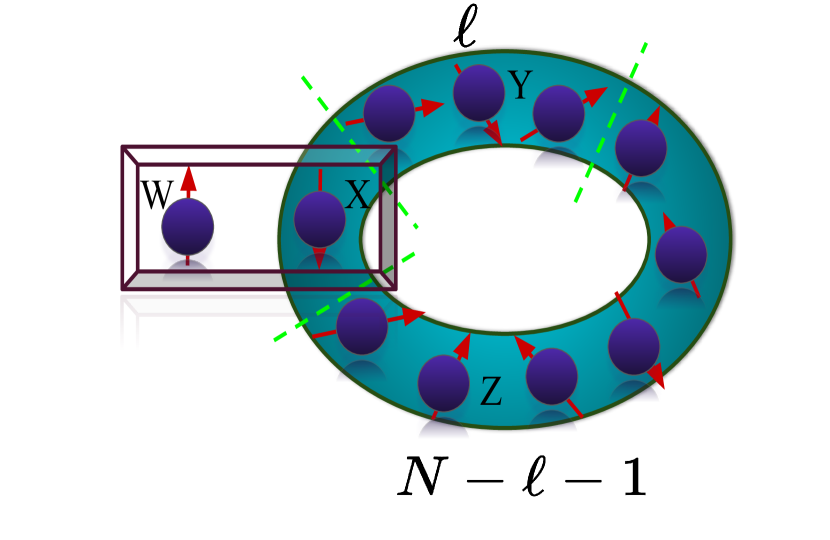
Figure 1: Illustration of our setup in which encoding and delocalization of information are represented. A chain of length $N$ with periodic boundary condition is divided into three parts: $X$, $Y$, and $Z$ of size $1$, $\ell$, and $N-\ell-1$, respectively. Initially, $W$ and $X$ are maximally entangled by the CNOT gate while $Y$ and $Z$ are not correlated with $W$ and $X$, however, $XYZ$ are entangled. Then, $XYZ$ evolves unitarily with a Hamiltonian and calculates the scrambling behavior in the entire spin system with time.

In the context of a single site within a spin system, we denote the spin-up state as $|\uparrow\rangle$ and the spin-down state as $|\downarrow\rangle$. These states are defined as follows:

$$|\uparrow\rangle=\begin{bmatrix}1\\ 0\end{bmatrix},~{}~{}~{}~{}~{}~{}~{}~{}~{}~{}~{}|\downarrow\rangle=\begin{bmatrix}0\\ 1\end{bmatrix}.$$ (2)

We prepare a three-party entangled product state $|\psi\rangle_{XYZ}$ and entangled it with state $W$ using CNOT gate. The combined state will be $|\phi\rangle$ and defined as

$$|\phi\rangle=\frac{1}{\sqrt{2}}(|\uparrow\rangle_{W}+|\downarrow\rangle_{W})\otimes|\psi\rangle_{XYZ},$$ (3)

If $W$ and $XYZ$ are not entangled then one will always have $I_{3}(W:Y:Z)=0$. After the entanglment between $W$ and $X$, $I_{3}(W:Y:Z)=I_{3}(X:Y:Z)$. When $I_{2}(X:Y)+I_{2}(X:Z)<I_{2}(X:YZ)$, TMI is negative, indicating that there is more information about $X$ contained in composite $YZ$ than there is in $Y$ and $Z$ separately which implies that information about $X$ is delocalized to $Y$ and $Z$. A more negative value of TMI indicates a higher degree of information delocalization. Measuring information about $X$ implies that $YZ$ is likely to unveil more about $X$ compared to $Y$ or $Z$ individually. In the calculation of TMI, we consider two types of product states. The first one is the all-up state that is given as

$$|\psi\rangle_{XYZ}=|\uparrow\uparrow\cdots\uparrow\uparrow\rangle,$$ (4)

and second one is Nèel state and which is defined as

$$|\psi\rangle_{XYZ}=|\uparrow\downarrow\uparrow\downarrow\cdots\uparrow\downarrow\rangle.$$ (5)

The saturation behavior of the TMI is intimately tied to the size of the subsystem $\ell$ under consideration. Specifically, when both subsystems, denoted as $Y$ and $Z$, possess identical sizes, the TMI reaches a saturation point at approximately the maximum negative value. However, as the size of either subsystem $Y$ or $Z$ decreases from this equal-size configuration, the TMI exhibits saturation at progressively less negative values. It is noteworthy that a more negative TMI value is indicative of a higher degree of scrambling within the system. In our TMI calculation, we do not observe an exact saturation of TMI; instead, there is an oscillation around a central value. To estimate this approximate central value, we utilize the following formula:

$$\overline{I_{3}(X:Y:Z)}=\frac{1}{T_{2}-T_{1}}\int_{T_{1}}^{T_{2}}I_{3}(X:Y:Z).$$ (6)

When examining the behavior of the TMI within discrete time intervals, the saturation of TMI is quantified by means of an average calculation. This calculation is expressed by the formula:

$$\overline{I_{3}(X:Y:Z)}=\frac{1}{T_{2}-T_{1}}\sum_{n=T_{1}}^{T_{2}}I_{3}(X:Y:Z),$$ (7)

where $T_{1}$ denotes the initial time point. Notably, we choose $T_{1}=100$ as a starting point since prior to this instance, the TMI exhibits dynamic behavior rather than being in the saturation regime. On the other hand, $T_{2}$ represents the final time point, which in our analysis is set to $T_{2}=500$. This approach enables us to quantitatively assess how the saturation behavior of the TMI changes with varying subsystem sizes. From now on, the notation $I_{3}(X:Y:Z)$ will be denoted as $\mathcal{I}_{3}$.

III Models

III.1 Transverse field Ising model

The transverse field Ising model (TFIM) is a specific variant of the Ising model that includes a transverse magnetic field, which is a perpendicular magnetic field applied to the spins in addition to the usual longitudinal magnetic field. The TFIM is particularly interesting because it exhibits quantum phase transitions Heyl et al. (2018); Su et al. (2006); Sun and Chen (2009) and quantum critical behavior, making it relevant in the study of quantum many-body systems and quantum computing. The Hamiltonian of the TFIM is given by:

$$\mathcal{\hat{H}}=J\hat{H}_{xx}+h_{x}\hat{H}_{x}+h_{z}\hat{H}_{z}.$$ (8)

The first term $J\hat{H}_{xx}$ represents the quantum spin-spin interaction energy in the $x-$ direction, similar to the classical spin interaction in the TFIM. The second term $h_{x}\hat{H}_{x}$ represents the energy due to an external magnetic field applied in the $x-$ direction (longitudinal magnetic field). The third term $h_{z}\hat{H}_{z}$ represents the energy due to an external magnetic field applied in the $z-$direction (transverse magnetic field). Only nearest-neighbor interactions are considered in the x-direction with periodic boundary condition, hence $\hat{H}_{xx}$ will be defined as $\hat{H}_{xx}=\sum_{i=1}^{N}\hat{\sigma}_{i}^{x}\sigma_{i+1}^{x}$, and $\hat{H}_{x/z}$ is defined as $\hat{H}_{x/z}=\sum\hat{\sigma}_{i}^{x/z}$, where $\hat{\sigma}_{i}^{x/z}$ represents the Pauli $X/Z$ matrix operator for the spin at site $i$. $J$ is the coupling constant that represents the strength of interaction between adjacent spins. $h_{x}/h_{z}$ is the strength of the continuous and constant longitudinal/transverse magnetic field.

A unitary operator is used to describe the time evolution of the quantum state of the system under the influence of the Hamiltonian. The time evolution operator, also known as the propagator, for a quantum system governed by a Hamiltonian $\mathcal{\hat{H}}$ defined by Eq. (8) is given as (taking $\hslash=1$):

$$\hat{U}(t)=\exp(-i\mathcal{\hat{H}}t)$$ (9)

In our numerical calculation, we will consider a case when the longitudinal field will be absent in the Hamiltonian $\mathcal{\hat{H}}$ [Eq. (8)]. Hereafter, corresponding to the presence and absence of a longitudinal magnetic field, we will call the systems nonintegrable and integrable TFIM, respectively.

III.2 Transverse field Ising Floquet spin system

A periodically kicked quantum Ising spin system, known as the quantum Ising Floquet spin system, is a variant of the transverse field Ising model. In this system, time-periodic magnetic fields are applied in the form of delta pulses in the transverse direction of the interaction of spins, and a continuous constant magnetic field is applied in the longitudinal direction of the interaction of spins. Hamiltonian of Floquet Ising model is given as:

$$\hat{H}(t)=J\hat{H}_{xx}+h_{x}\hat{H}_{x}+h_{z}\sum_{n=-\infty}^{\infty}\delta\Big{(}n-\frac{t}{\tau}\Big{)}\hat{H}_{z}.$$ (10)

All terms in Eq. (10) are identical to those in Eq. (8), except for the Dirac delta term. In Eq. (10), $h_{z}$ represents the strength of the kicking field, $\tau$ is referred to as the Floquet period, and $n$ is the number of kicks applied.

The operator that evolves states is the quantum map, defined for one period of time $\tau$

$$\mathcal{\hat{U}}=e^{-i\tau(J\hat{H}_{xx}+h_{x}\hat{H}_{x})}e^{-i\tau h_{z}\hat{H}_{z}}$$ (11)

For $n$ ($t=n\tau$) number of kicks, Floquet map will be $\hat{U}_{F}(t=n\tau)=(\mathcal{\hat{U}})^{n}$, and called it as n-propagator. The presence, simultaneously, of longitudinal and transverse field terms makes the model nonintegrable. The absence of longitudinal magnetic fields makes the model integrable. Thereafter, we will call it an integrable $\mathcal{\hat{U}}_{0}$ system and nonintegrable $\mathcal{\hat{U}}_{x}$ system for integrable and nonintegrable Floquet systems.

Periodic Hamiltonian has attracted a lot of attention among researchers for a very long time Kapitza et al. (1951); Chirikov (1971); Casati et al. (1979). In recent years, Floquet spin systems with constant fields Gritsev and Polkovnikov (2017); Lakshminarayan and Subrahmanyam (2005); D’Alessio and Rigol (2014); Naik et al. (2019); Shukla et al. (2021); Mishra et al. (2015) and quenched fields Mishra and Lakshminarayan (2014); Rossini et al. (2010); Essler and Fagotti (2016); Russomanno et al. (2012, 2013) got considerable attention. In experiments to describe certain properties of matter, periodic perturbation can be realized Ovadyahu (2012); Iwai et al. (2003); Kaiser et al. (2014); Ammann et al. (1998).

IV Results

Our research aims to investigate the scrambling behavior within the TFIM and Floquet model, exploring both integrable and nonintegrable scenarios. Given that the dynamics of scrambling are influenced by the initial state, we will examine two distinct starting configurations: the fully aligned “all-up” state and the alternating “Nèel” state defined by Eq. (4) and Eq. (5), respectively. Our focus will encompass both the initial time dynamics, which involve quantifying the rate at which information becomes scrambled as the system evolves, and the late time dynamics, which describe the degree of scrambling. To achieve this, we will employ the concept of TMI to measure the extent of correlations and entanglement between different components of the system. By utilizing numerical simulations using exact diagonalisation computational techniques, we will calculate the TMI over time. Our objective is also to analyze and contrast the scrambling behavior of the TFIM in comparison to the Floquet model, with a specific focus on highlighting the advantages of incorporating the Floquet system.

IV.1 Transverse Field Ising Model

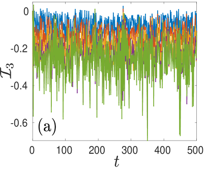
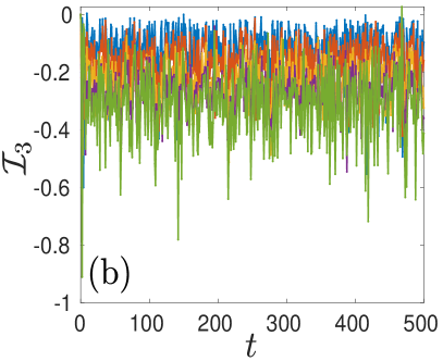
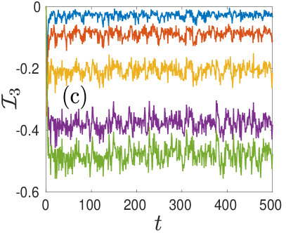
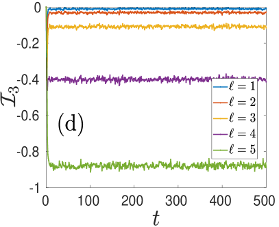
Figure 2: $\mathcal{I}_{3}$ vs $t$ for TFIM without longitudinal field (a, b) and with longitudinal field (c, d). The initial state is all upstate in cases (a, c), while the Néel state in cases (b, d). Parameters: $J=1$, $h_{z}=1$, $h_{x}=0/1$, $N=11$ with periodic boundary conditions.

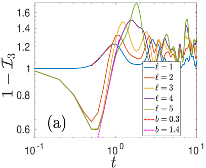
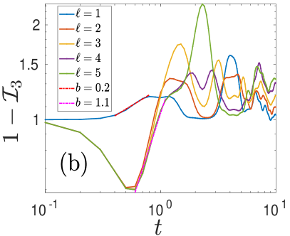
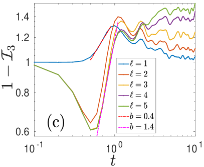
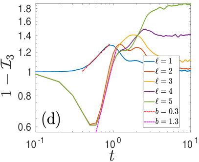
Figure 3: $1-\mathcal{I}_{3}$ vs $t$ ($\log-\log$) for TFIM without longitudinal field (a, b) and with longitudinal field (c, d). The initial state is all upstate in cases (a, c), while the Néel state in cases (b, d). Parameters: $J=1$, $h_{z}=1$, $h_{x}=0/1$, $N=11$ with periodic boundary conditions. Dashed lines represent the polynomial fitting.

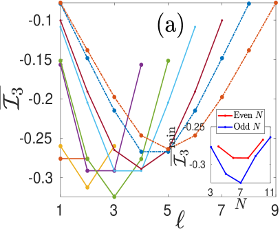
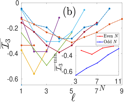
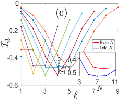
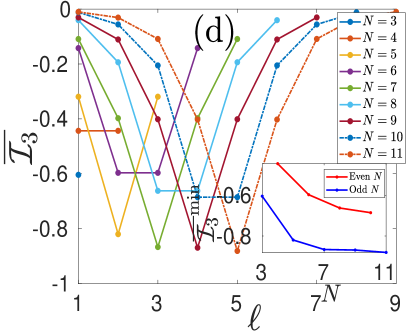
Figure 4: $\overline{\mathcal{I}}_{3}$ vs $\ell$ in TFIM without longitudinal field (a, b) and with longitudinal field (c, d) for different $N$ ranging from $3$ to $11$. The initial state is all upstate in cases (a, c), while the Néel state in cases (b, d). Parameters: $J=1$, $h_{z}=1$, $h_{x}=0/1$, $N=11$ with periodic boundary conditions. The inset illustrates minima of $\mathcal{I}_{3}$ in relation to $N$. These minima are displayed separately for even (red solid line) and odd (blue solid line) values of $N$.

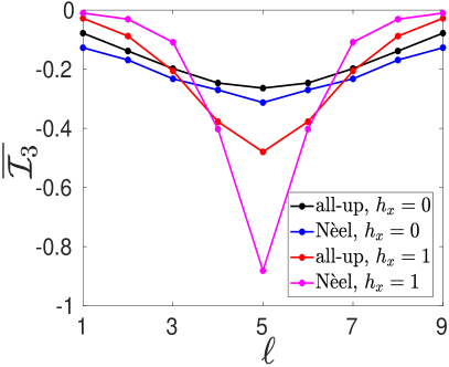
Figure 5: $\overline{\mathcal{I}}_{3}$ vs $\ell$ in the TFIM for all four cases which considered in Fig. 4, while keeping a fix $N=11$, with all parameters held same.

We have observed the emergence of negative TMI values in both integrable and nonintegrable TFIM at all time steps, except for some small initial time points. This trend is consistent across both initial states, as illustrated in Fig. 2. When comparing the integrable [Fig. 2 (a, b)] and nonintegrable TFIM cases [Fig. 2 (c, d)], we observe distinct behaviors in terms of the oscillation amplitude. Smaller oscillations tend to yield more precise results. In the integrable scenario, the oscillation amplitude is notably larger. In contrast, the nonintegrable case exhibits much smaller oscillation amplitudes. Additionally, upon comparing the two initial states, we note that the Nèel state [Fig. 2 (b, d)] displays fewer oscillations compared to the all-up state [Fig. 2 (a, c)]. In all cases, as the subsystem size $\ell$ increases, TMI oscillates around increasingly negative values, indicating a greater degree of information scrambling.

To capture the initial growth of scrambling, we introduce the quantity $1-\mathcal{I}_{3}$, which ensures that all values on the y-axis are positive. While, in our calculation, $\mathcal{I}_{3}$ values lie between $1$ and $-1$, the range for $1-\mathcal{I}_{3}$ spans from $0$ to $2$. This transformation allows us to effectively examine the power-law growth of TMI. Upon conducting our analysis, we make a noteworthy observation: both the integrable and nonintegrable TFIM, for both initial states, exhibit power-law growth of scrambling i.e., $(1-\mathcal{I}_{3})\propto t^{b}$. This behavior is demonstrated in Fig. 3. When considering the subsystem $Y$ of size, $\ell=1$, we find that the power-law exponent is quite small ($b\approx 0.3$). However, for all other subsystem size, the exponent is large ($b\approx 1.3$) and approximately equal for all subsystem size $\ell\neq 1$. For $\ell=1$, we observe that $\mathcal{I}_{3}$ remains at zero for some initial small time, after which it converges towards negative values. This observation implies an absence of initial information propagation during the early time, with subsequent information delocalization throughout the system. In the case of $\ell\neq 1$, we obtain a positive value of $\mathcal{I}_{3}$ for some initial time, followed by a decrease towards negative values. This implies that for a small initial time, information is localized and then becomes delocalized. This behavior is influenced by periodic boundary conditions in the spin chain. With $\ell=1$, most of the information flows in one direction, similar to the case of open boundary conditions Iyoda and Sagawa (2018). However, when $\ell\neq 1$, information propagates from both directions of the spin chain, resulting in a positive value of $\mathcal{I}_{3}$ during the initial time regime. After some time, it decreases toward negative values. This implies that information is initially localized, and then it begins to delocalize throughout the system. By altering the subsystem sizes of both $Y$ and $Z$, the rate of information flow remains unaffected. This is because the flow of information compensates in one direction with the flow from the other direction. Consequently, this situation results in approximately equal exponent values for all $\ell\neq 1$.

The saturation behavior of $\mathcal{I}_{3}$ characterizes the degree of scrambling. A more negative value of $\mathcal{I}_{3}$ corresponds to a more scrambled system, meaning that the information is highly delocalized. There is no precise saturation point for $\mathcal{I}_{3}$. Instead, it is distinguished by oscillations around a central value, without truly reaching a saturation point. To determine the central value around which $\mathcal{I}_{3}$ oscillates, we calculate the integration of the saturation values of $\mathcal{I}_{3}$ by using Eq. (6). Our investigation involves studying the value of $\overline{\mathcal{I}}_{3}$ as we increment the subsystem size $\ell$ for various system sizes $N$. Notably, the saturation value of $\mathcal{I}_{3}$ is influenced by the size of the system $N$. We unveil intriguing differences between cases of odd and even system sizes. When $N$ is odd, $\overline{\mathcal{I}}_{3}$ exhibits its highest negative value at $\ell=(N-1)/2$. This behavior arises due to the symmetrical alignment of subsystem sizes $Y$ and $Z$ in odd-N configurations. In the case of even $N$, this minimum value of $\overline{\mathcal{I}}_{3}$ is achieved at $\ell=(N-2)/2$. $\overline{\mathcal{I}}_{3}$ provide symmetric behavior about $\ell=(N-1)/2$ in case of odd $N$ and about a straight line lies between $\ell=(N-2)/2$ and $\ell=N/2$ in the case of even $N$ [Fig. 4]. This behavior is a result of the relationship between the subsystem sizes, where $Y$ has a length of $\ell$ and $Z$ has a length of $N-\ell-1$ in a spin chain of total length $N$. In the case of an odd $N$, when we extend the subsystem size of $Y$ beyond $\ell=(N-1)/2$, the size of subsystem $Z$ mirrors the previous size of $Y$. However, in the case of an even $N$, when the subsystem size of $Y$ is $\ell=(N-2)/2$, the size of subsystem $Z$ becomes $N/2$. When we increase the size of subsystem $Y$ to match $\ell=N/2$, the size of subsystem $Z$ aligns with the previous size of $Y$. As a result, at these two sizes of $Y$, $\overline{\mathcal{I}}_{3}$ assumes the same value. Comparing the higest negative values of $\overline{\mathcal{I}}_{3}$ for a fixed $N$, a noteworthy distinction emerges: odd $N$ manifest a higher negative value of $\overline{\mathcal{I}}_{3}$ at $\ell=(N-1)/2$. This result can be attributed to specific combinations in odd system sizes where subsystem sizes of $Y$ and $Z$ become equivalent, resulting in heightened scrambling scenarios. However, a similar scenario does not occur within even $N$. A distinctive pattern emerges when comparing the values of $\overline{\mathcal{I}}_{3}$ for odd and even $N$. Odd system sizes consistently yield more negative values than their nearest-even counterparts. Visualizing the highest negative values of $\overline{\mathcal{I}}_{3}$ for even and odd $N$, it becomes evident that the curve corresponding to odd $N$ lies below that of even $N$. This trend is depicted in the inset of Fig. 4. In the context of both the integrable and nonintegrable TFIM scenarios with an all-up initial state, we observe a pattern where the highest negative value of $\overline{\mathcal{I}}_{3}$ (both odd and even $N$) initially decreases with increasing $N$, but after reaching a certain fixed value of $N$, they begin to increase [see Fig. 4(a) and (c)]. However, in the case of the integrable TFIM with a Néel initial state, $\overline{\mathcal{I}}^{\rm min}_{3}$ exhibit an opposite trend: they increase as $N$ increases [see Fig. 4(b)]. In nonintegrable TFIM with the Néel state as the initial condition, a notable trend emerges: $\overline{\mathcal{I}}^{\rm min}_{3}$ diminishes as the $N$ increases. This intriguing behavior hints at a significant prediction: as $N$ approaches $\infty$, $\overline{\mathcal{I}}^{\rm min}_{3}$ expected to converge towards $-1$ i.e., $N\rightarrow\infty\implies\overline{\mathcal{I}}^{\rm min}_{3}\rightarrow-1$. This behavior is depicted in the inset of Fig. 4(d).

Conducting a comprehensive comparison across all cases for $N=11$, we discern distinct levels of scrambling within the studied scenarios. In cases where there exists a substantial disparity in the sizes of subsystems $Y$ and $Z$, the integrable TFIM tends to yield a notably more negative value for the quantity $\overline{\mathcal{I}}_{3}$ when compared to the nonintegrable TFIM. As the disparity in the sizes of subsystems $Y$ and $Z$ decreases, the nonintegrable TFIM tends to approach a more negative value for $\overline{\mathcal{I}}_{3}$ in comparison to the integrable TFIM. Specifically, for $\ell=(N-1)/2$, within the integrable TFIM, the system initialized in the all-up state exhibits the least degree of scrambling. Contrarily, when considering the Néel state as the initial configuration, a heightened level of scrambling is observed. Shifting our focus to the nonintegrable TFIM, the dynamics take on a different character. In this context, the Néel state surpasses the all-up state in terms of scrambling intensity. Remarkably, this implies that the Néel state in the nonintegrable TFIM manifests as the most potent scrambler among the cases studied [Fig. 5]. These findings provide a compelling picture of the intricate relationships between system integrability, initial states, and the degree of information scrambling within the TFIM.

IV.2 Transverse field Ising Floqeut spin system

IV.2.1 Scrambling at small period $\tau=\epsilon/2$

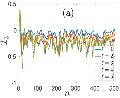
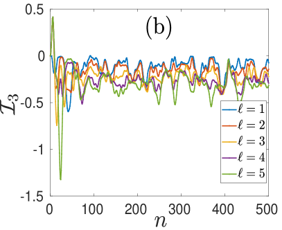
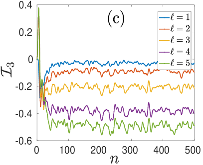
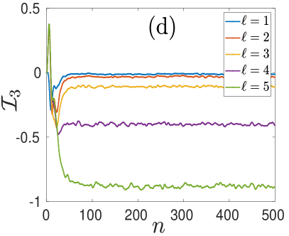
Figure 6: $\mathcal{I}_{3}$ vs $n$ in Floquet Ising spin system at period $\tau=\epsilon/2~{}(\epsilon=\pi/16)$ without longitudinal field (a, b) and with longitudinal field (c, d). The initial state is all upstate in cases (a, c), while the Néel state in cases (b, d). Parameters: $J=1$, $h_{z}=1$, $h_{x}=0/1$, $N=11$ with periodic boundary conditions.

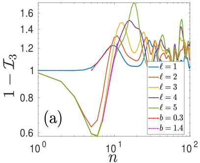
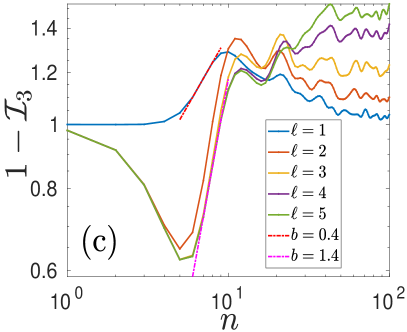
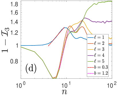
Figure 7: $1-\mathcal{I}_{3}$ vs $n$ ($\log-\log$) in Floquet system at period $\tau=\epsilon/2$ without longitudinal field (a, b) and with longitudinal field (c, d). The initial state is all upstate in cases (a, c), while the Néel state in cases (b, d). Parameters: $J=1$, $h_{z}=1$, $h_{x}=0/1$, $N=11$ with periodic boundary conditions. Dashed lines represent the polynomial fitting.

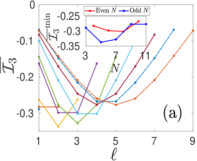
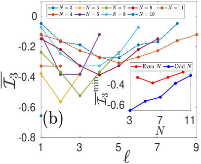
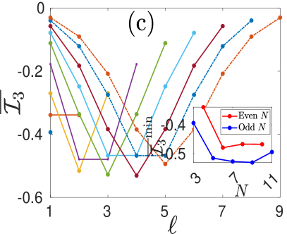
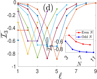
Figure 8: $\overline{\mathcal{I}}_{3}$ vs $\ell$ in Floquet system at period $\tau=\epsilon/2$ without longitudinal field (a, b) and with longitudinal field (c, d) for different $N$ ranging from $3$ to $11$. The initial state is all upstate in cases (a, c), while the Néel state in cases (b, d). Parameters: $J=1$, $h_{z}=1$, $h_{x}=0/1$, $N=11$ with periodic boundary conditions. The inset illustrates minima of $\overline{\mathcal{I}}_{3}$ in relation to $N$. These minima are displayed separately for even (red solid line) and odd (blue solid line) values of $N$.

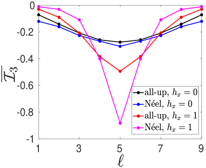
Figure 9: $\overline{\mathcal{I}}_{3}$ vs $\ell$ in the Floquet system for all four cases which are considered in Fig. 8, while keeping fix $N=11$, with all parameters held same.

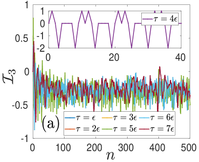
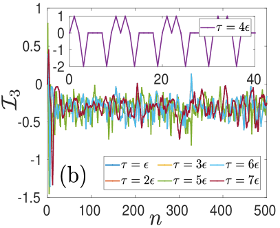
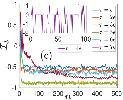
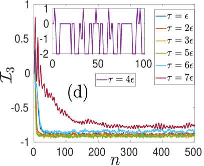
Figure 10: $\mathcal{I}_{3}$ vs $n$ for Floquet system with an increasing period ranging from $0$ to $\pi/2$ differing by $\epsilon~{}(\epsilon=\pi/16)$ without longitudinal field (a, b) and with longitudinal field (c, d). The initial state is all upstate in cases (a, c), while the Néel state in cases (b, d). Parameters: $J=1$, $h_{z}=1$, $h_{x}=0/1$, $N=11$ with periodic boundary conditions.

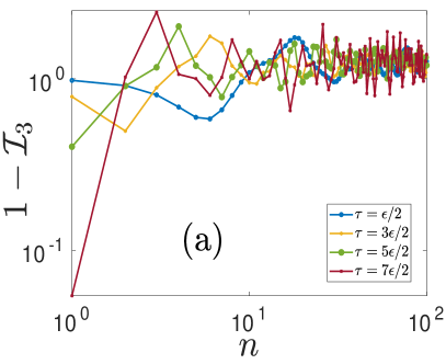
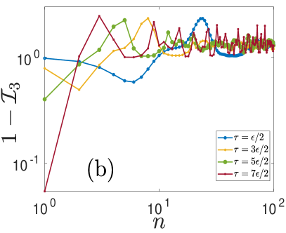
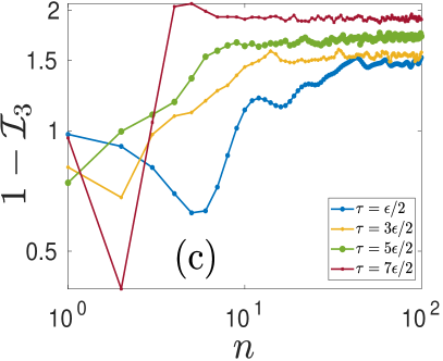
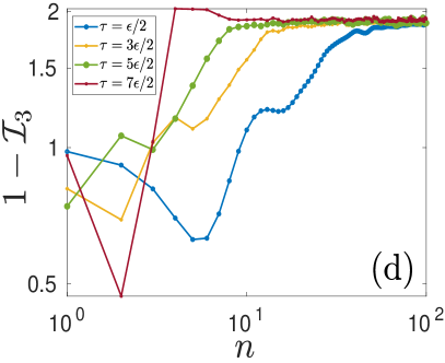
Figure 11: $1-\mathcal{I}_{3}$ vs $n$ for Floquet system with an increasing period ranging from $0$ to $\pi/2$ differing by $\epsilon~{}(\epsilon=\pi/16)$ without longitudinal field (a, b) and with longitudinal field (c, d). The initial state is all upstate in cases (a, c), while the Néel state in cases (b, d). Parameters: $J=1$, $h_{z}=1$, $h_{x}=0/1$, $N=11$ with periodic boundary conditions.

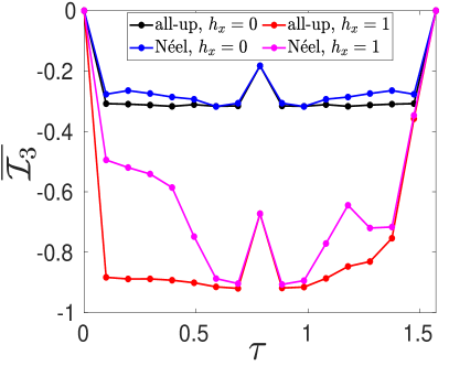
Figure 12: $\overline{\mathcal{I}}_{3}$ vs $\tau$ in the Floquet system of size $N=11$ and subsystemsize $\ell=(N-1)/2$ for all four cases which considered in Fig. 11, with all parameters held same.

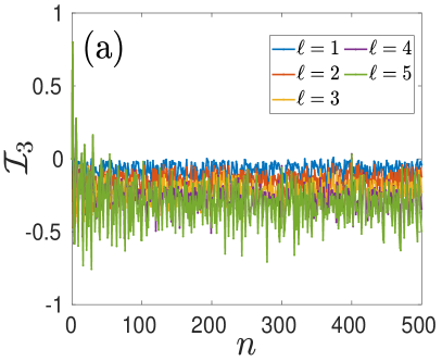
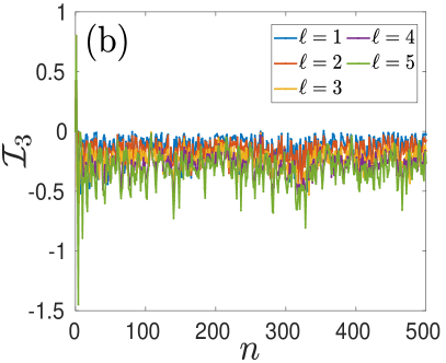
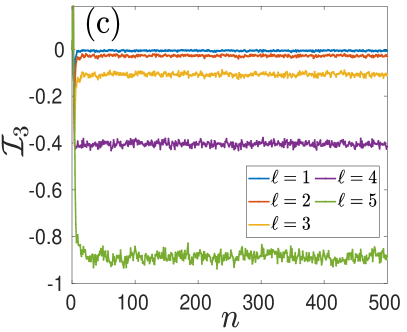
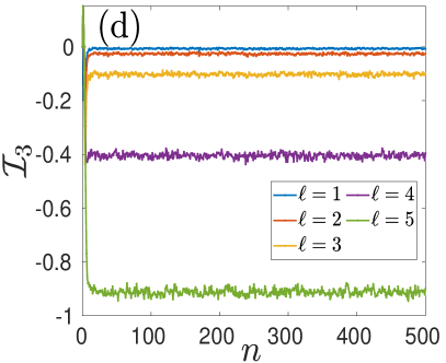
Figure 13: Similar to Fig. 6, but considering a period of $\tau=6\epsilon/2$.

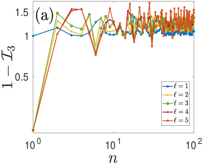
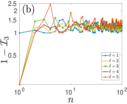
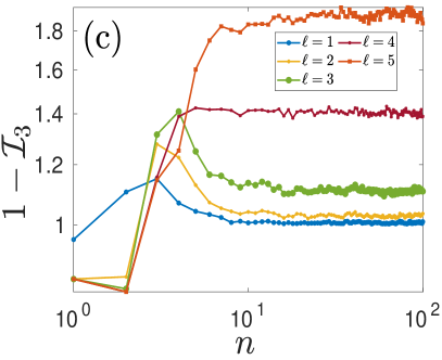
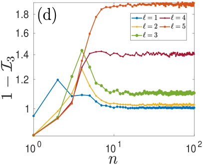
Figure 14: Similar to Fig. 7, but considering a period of $\tau=6\epsilon/2$.

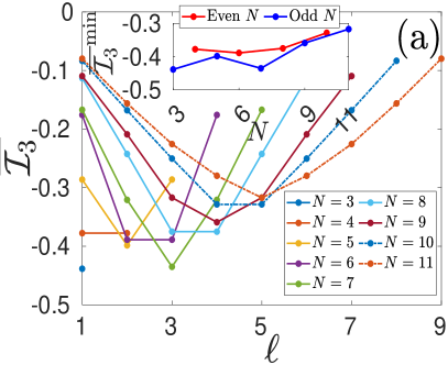
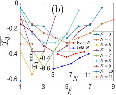
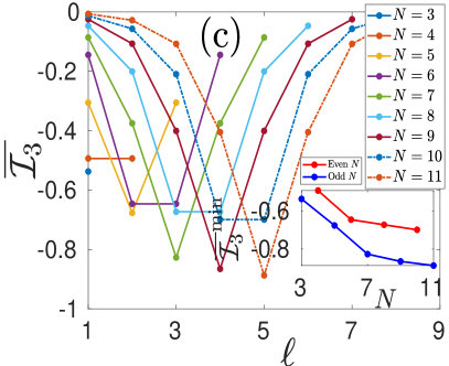
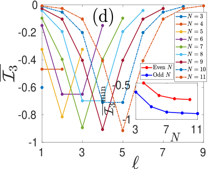
Figure 15: Similar to Fig. 8, but considering a period of $\tau=6\epsilon/2$.

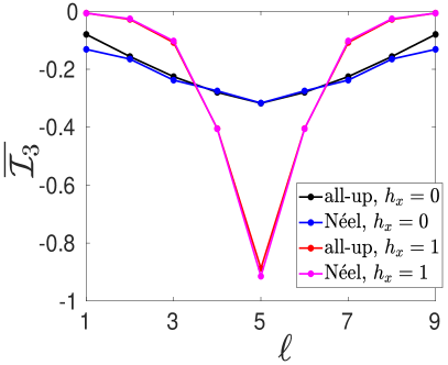
Figure 16: $\overline{\mathcal{I}}_{3}$ vs $\ell$ in the Floquet system for all four cases which are considered in Fig. 15, while keeping fix $N=11$, with all parameters held same.

We delve into the exploration of scrambling within both integrable and nonintegrable Floquet systems. Our investigation spans various subsystem sizes ($\ell$), with a specific focus on a short Floquet period, $\tau=\epsilon/2$ $(\epsilon=\pi/16)$. At this swift Floquet period, intriguingly, the behavior of the unitary operator mirrors that of the TFIM. This alignment in behavior emerges due to the rapid nature of the kicks—when the kicking is exceptionally fast, the system lacks the time to relax, resembling a scenario akin to TFIM. In both integrable $\mathcal{\hat{U}}_{0}$ and nonintegrable $\mathcal{\hat{U}}_{x}$ systems, TMIs exhibit negative values throughout all time regimes, except for some initial kicks, as shown in Fig. 6. In both integrable $\mathcal{\hat{U}}_{0}$ and nonintegrable $\mathcal{\hat{U}}_{x}$ systems, TMIs do not reach a specific saturation value but instead exhibit oscillations around a certain central value. This central value tends towards a more negative value as the size of the subsystem $\ell$ increases. When we compare the integrable $\mathcal{\hat{U}}_{0}$ system with the nonintegrable $\mathcal{\hat{U}}_{x}$ system, we observe that the oscillation amplitude is significantly smaller in the nonintegrable $\mathcal{\hat{U}}_{x}$ system. Additionally, in the nonintegrable $\mathcal{\hat{U}}_{x}$ system, the degree of scrambling is more as compared to the integrable case. In the nonintegrable $\mathcal{\hat{U}}_{x}$ system with initial Néel state, the TMIs display minimal oscillations and tend to settle at even more negative values as compared to all other cases, especially at $\ell=(N-1)/2$[Fig. 6(d)]. In the context of the Floquet system, the negative values of $\mathcal{I}_{3}$ observed in all time regimes align with the behavior observed in the TFIM case. However, The oscillation amplitude during the saturation regime of $\mathcal{I}_{3}$ is smaller in the Floquet system compared to the TFIM case.

To capture the initial growth patterns of $\mathcal{I}_{3}$ in the Floquet system with a small period $\tau=\epsilon/2$, we employ the calculation of $1-\mathcal{I}_{3}$, similar to the TFIM case. Remarkably, $1-\mathcal{I}_{3}$ exhibits power-law growth behavior within both the integrable and nonintegrable Floquet systems i.e., $(1-\mathcal{I}_{3})\propto t^{b}$, as depicted in Fig. 7. In both the integrable $\mathcal{\hat{U}}_{0}$ and nonintegrable $\mathcal{\hat{U}}_{x}$ systems, the power-law exponent is relatively small, around $b\approx 0.3$ when $\ell=1$. However, for all $\ell\neq 1$, the exponent of the power-law growth is notably larger, around $b\approx 1.3$. These exponents are approximately similar to those observed in the TFIM case.

Similarly to the TFIM case, in the Floquet system, $\mathcal{I}_{3}$ doesn’t converge to a specific value but rather displays oscillations around a central value. Given that the Floquet system is discrete, integration as used in the TFIM case is not applicable here. Instead, we resort to average of $\mathcal{I}_{3}$ over a range, covering the interval from $T_{1}=100$ to $T_{2}=500$, as presented in Eq. 7. The saturation of $\mathcal{I}_{3}$ is influenced by both the subsystem size $\ell$ and the system size $N$, following patterns similar to those observed in the TFIM case. These trends differ depending on whether the system size is even or odd. Specifically, in the case of odd $N$, the negative value of $\overline{\mathcal{I}}_{3}$ increases until it reaches a critical threshold at $\ell=(N-1)/2$. For even $N$, the threshold occurs at $\ell=(N-2)/2$. $\overline{\mathcal{I}}_{3}$ exhibits symmetric behavior around $\ell=(N-1)/2$ for odd $N$ and around a line drawn between $\ell=(N-2)/2$ and $\ell=N/2$ for even $N$. When considering the maximum negative of $\overline{\mathcal{I}}_{3}$ for all $N$ and plotting them against $N$, we observe different trends for odd and even $N$. Remarkably, odd $N$ consistently yields a higher degree of scrambling compared to even $N$. This systematic behavior is depicted in the inset of Fig. 8. In the case of the integrable $\hat{\mathcal{U}}_{0}$ system, the minima of $\overline{\mathcal{I}}_{3}$ exhibit an upward trend as $N$ increases for both initial states [Fig. 8(a) and (b)]. However, in the nonintegrable $\hat{\mathcal{U}}_{x}$ system with an all-up initial state, the minima of $\overline{\mathcal{I}}_{3}$ initially decrease with increasing $N$ but eventually start to increase after reaching a certain fixed value of $N$ [ Fig. 8(c)]. Notably, there is a consistent pattern in the behavior of $\overline{\mathcal{I}}^{\rm min}_{3}$ in the case of the nonintegrable $\mathcal{\hat{U}}_{x}$ system with Néel state for both odd and even $N$. As $N$ increases, $\overline{\mathcal{I}}^{\rm min}_{3}$ gradually approaches $-1$. Consequently, it can be inferred that as $N\rightarrow\infty$, $\overline{\mathcal{I}}^{\rm min}_{3}$ will converge towards the value of $-1$ [Fig. 8(d)]. This behavior is in alignment with what is observed in the TFIM case.

A comparative analysis of $\overline{\mathcal{I}}_{3}$ across all four cases, with a fixed $N=11$, reveals intriguing distinctions. In the case of the integrable $\mathcal{\hat{U}}_{0}$ system, $\overline{\mathcal{I}}_{3}$ follows a comparable pattern for both initial states, with a notably more negative value observed when starting from the Néel state. However, in the nonintegrable $\mathcal{\hat{U}}_{x}$ system, $\overline{\mathcal{I}}_{3}$ takes on a significantly more negative value when starting from the Néel state, in comparison to the all-up state at $\ell=(N-1)/2$ and its nearest neighbor. For all other values of $\ell$, $\overline{\mathcal{I}}_{3}$ exhibits less negative values in the case of the Néel state. Furthermore, for smaller $\ell$, the integrable $\mathcal{\hat{U}}_{0}$ system displays a more negative value of $\overline{\mathcal{I}}_{3}$ in comparison to the nonintegrable $\mathcal{\hat{U}}_{x}$ system. As the subsystem size $\ell$ approaches $(N-1)/2$, the negative value of $\overline{\mathcal{I}}_{3}$ increases notably in the case of the nonintegrable $\mathcal{\hat{U}}_{x}$ system, as illustrated in Fig. 9. This behavior closely resembles the trends observed in the TFIM cases.

IV.2.2 Scrambling across the period $0$ to $\pi/2$

We embark on an extensive investigation of the scrambling in the Floquet system, covering a range of periods from $0$ to $\pi/2$ in increments of $\pi/16$, encompassing all four distinct cases. Throughout this study, the $\mathcal{I}_{3}$ consistently exhibit negative values for all periods, as illustrated in Fig. 10. However, there is an exception at $\tau=\pi/4$, clearly depicted in the inset of Fig. 10. At this specific period of $\tau=\pi/4$, $\mathcal{I}_{3}$ displays a periodic behavior. Intriguingly, the period of this oscillation seamlessly aligns with the system size, $N$. In the integrable $\mathcal{\hat{U}}_{0}$ system, the period is straightforward and equal to $N$. However, in the nonintegrable $\mathcal{\hat{U}}_{x}$ system, a more complex connection exists. At this period, in both integrable $\mathcal{\hat{U}}_{0}$ and nonintegrable $\mathcal{\hat{U}}_{x}$ system, $\mathcal{I}_{3}$ oscillates between the values of $-2$ and $1$. This behavior implies that during this period, the system does not exhibit scrambling behavior at all times.

To quantify the scrambling growth rate within the range of periods spanning from $0$ to $\pi/2$, we have calculated the quantity $1-\mathcal{I}_{3}$. Our results consistently demonstrate that scrambling exhibits power-law growth for all periods, as illustrated in Fig. 11. As we increase the period, the growth rate also increases, eventually reaching a saturation region with fewer kicks. In the vicinity of $\tau=\pi/4~{}(\tau=7\epsilon/2)$, there is a noticeable sudden jump in the behavior.

We conducted a comprehensive analysis by computing $\overline{\mathcal{I}}_{3}$ across periods from $0$ to $\pi/2$, with increments of $\epsilon/2$, for a system with $N=11$ and $\ell=(N-1)/2$. This investigation allowed us to make comparisons across all considered cases. In the integrable $\mathcal{\hat{U}}_{0}$ system, we observed that $\overline{\mathcal{I}}_{3}$ typically has small negative values for the Néel state compared to the all-up state across all Floquet periods except at $\tau=\pi/4$. Intriguingly, at $\tau=\pi/4$, $\overline{\mathcal{I}}_{3}$ becomes exactly the same for both initial states. When we compare the nonintegrable $\mathcal{\hat{U}}_{x}$ system, we find that $\overline{\mathcal{I}}_{3}$ tends to exhibit less negative values for the Néel state when compared to the all-up state for most periods, except at $\tau=\pi/4$, where $\overline{\mathcal{I}}_{3}$ takes on the same value for both initial states. Notably, in the nonintegrable $\mathcal{\hat{U}}_{x}$ system, $\overline{\mathcal{I}}_{3}$ consistently shows more negative values for all periods within the range of $0$ to $\pi/2$ when compared to the integrable $\mathcal{\hat{U}}_{0}$ system [Fig. 12]. This periodic behavior of $\overline{\mathcal{I}}_{3}$ is symmetric about $\tau=\pi/4$ in the case of the integrable $\mathcal{\hat{U}}_{0}$ system, as the unitary operator exhibits the same behavior for periods $\tau$ and $\pi/2-\tau$ Shukla et al. (2021).

IV.2.3 Scrambling in the vicinity of $\tau=\pi/4$

When we conduct an analysis of $\overline{\mathcal{I}}_{3}$ across various periods within the range of $0$ to $\pi/2$, we notice that the most degree of scrambling emerges in proximity to the period $\tau=\pi/4$. These intriguing characteristics motivate us to investigate the behavior of scrambling in the vicinity of the period $\tau=\pi/4$. Therefore, we have computed $\mathcal{I}_{3}$ for a period $\tau$ equal to $\frac{6\epsilon}{2}$, where $\epsilon$ is set to $\frac{\pi}{16}$. Within the context of integrable scenarios, $\mathcal{I}_{3}$ exhibit oscillations with a similar amplitude as those observed for a smaller period, $\tau=\frac{\epsilon}{2}$. Upon conducting a thorough analysis across nonintegrable cases, we observe that the oscillations are less pronounced compared to what is evident in situations involving shorter Floquet periods. This intriguing phenomenon is clearly illustrated in Fig. 13. This collective observation emphasizes the impact of the duration of the Floquet period on the amplitude of oscillations in the TMI, particularly in nonintegrable systems.

We have conducted an analysis of the initial growth of the scrambling using quantity $1-\mathcal{I}_{3}$. This measure exhibits a sudden jump after the first/second kick in the $\hat{\mathcal{U}}_{0}$/$\hat{\mathcal{U}}_{x}$ systems followed by saturation [Fig. 14]. This pattern indicates a very rapid growth rate.

We have computed $\overline{\mathcal{I}}_{3}$ for all combinations of $\ell$ in different system sizes ($N$) in both integrable and nonintegrable Floquet systems with a period of $\tau=6\epsilon/2$. All cases have similar behavior of $\overline{\mathcal{I}}_{3}$ and $\overline{\mathcal{I}}^{\rm min}_{3}$ as small period, $\tau=\epsilon/2$ [Fig. 15].

In our comprehensive study of $\overline{\mathcal{I}}_{3}$ for all the cases considered at a period of $\tau=\frac{6\epsilon}{2}$, with a fixed $N=11$, we observe similar behavior to that seen during the smaller period $\tau=\epsilon/2$. However, during this period, $\overline{\mathcal{I}}_{3}$ consistently remains the same for both initial states in both the integrable $\mathcal{\hat{U}}_{0}$ and the non-integrable $\mathcal{\hat{U}}_{x}$ systems, as shown in Fig. 16. Notably, in the nonintegrable $\hat{\mathcal{U}}_{x}$ system with an all-up state, $\overline{\mathcal{I}}_{3}$ exhibits more negative values when compared to the behavior during the shorter time period $\tau=\epsilon/2$ at $\ell=(N-1)/2$ (Compare Fig. 9 and Fig. 16).

V Conclusion

Our study delves deeply into the quantum information scrambling phenomena within both integrable and nonintegrable TFIM and Floquet systems under closed boundary conditions. To characterize the scrambling behavior, we employ the TMI as a measure to track the extent of quantum information delocalization throughout the system. Specifically, we focus on negative TMI values as an indicator of enhanced scrambling. Recognizing that scrambling behavior can depend on the initial state, we carefully examine two distinct scenarios: one where the system is initialized with an all-up state and another with a Néel state.

In our initial investigation, we concentrate on the TFIM framework. Our calculations reveal a consistent negative trend in TMI across all subsystem sizes for both integrable and nonintegrable TFIM, regardless of the chosen initial states. This suggests that the system exhibits scrambling behavior in all the considered cases. Additionally, we explore the initial growth of scrambling, which intriguingly exhibits power-law patterns in both integrable and nonintegrable TFIM cases. Expanding our analysis, we compute the average of TMI ($\overline{\mathcal{I}}_{3}$) across various system sizes to describe the saturation behavior of TMI. $\overline{\mathcal{I}}_{3}$ becomes more negative as the subsystem size $\ell$ increases. It reaches its most negative value at $\ell=(N-1)/2$ for odd values of $N$ and at $(N-2)/2$ for even values of $N$. The minima of $\overline{\mathcal{I}}_{3}$ exhibit distinct trends in systems with even and odd sizes, with the plot for odd $N$ consistently lying below that for even $N$. A key observation emerges when comparing integrable and nonintegrable TFIM scenarios: at subsystem size $\ell=(N-1)/2$, the system has a higher degree of scrambling in a nonintegrable context. Notably, in the nonintegrable TFIM framework with a Néel state initialization, $\overline{\mathcal{I}}_{3}$ approaches a value of $-1$ as $N$ tends towards infinity, indicating heightened scrambling tendencies.

Shifting our focus to the Floquet model, we first examine a short period, as the Floquet model exhibits similarities to TFIM. The overarching patterns consistently persist: negative TMI values dominate in both integrable and nonintegrable Floquet systems, regardless of the initial states. In the integrable $\mathcal{\hat{U}}_{0}$ system, oscillation amplitudes are nearly similar to TFIM. However, in the nonintegrable $\mathcal{\hat{U}}_{x}$ system, oscillation amplitudes are less pronounced compared to TFIM. The power-law growth pattern of TMI remains intact, with approximately the same exponent as observed in TFIM. In the nonintegrable Floquet framework, for $\ell=(N-1)/2$ and its nearest neighbor, we observe more negative values of $\overline{\mathcal{I}}_{3}$ compared to their counterparts in the integrable $\mathcal{\hat{U}}_{0}$ system. Notably, in the nonintegrable $\mathcal{\hat{U}}_{x}$ system, initiating with a Néel state results in heightened scrambling tendencies.

Our analysis regarding scrambling behavior covers a range of Floquet periods from $0$ to $\pi/2$. At all periods $\mathcal{I}_{3}$ has a negative value except $\tau=\pi/4$, where TMI demonstrates a distinctive periodic pattern, oscillating between $-2$ and $1$. This finding sparks a heightened interest in further investigating this critical period. For all periods except $\tau=\pi/4$, the initial growth of scrambling follows a power-law pattern. The growth rate of scrambling accelerates as the period increases, and in proximity to the $\pi/4$ period, a notable and abrupt jump is observed. As the period is extended, $\mathcal{I}_{3}$ requires fewer kicks to approach saturation. This implies that increasing the period enhances the growth rate of scrambling. In addition, when analyzing the average TMI ($\overline{\mathcal{I}}_{3}$) across all periods ranging from $0$ to $\pi/2$, with increments of $\epsilon/2$, we observe that $\overline{\mathcal{I}}_{3}$ exhibits less negative values in the case of the integrable $\mathcal{\hat{U}}_{0}$ system in comparison to the nonintegrable $\mathcal{\hat{U}}_{x}$ system. As the period increases, the negative value of $\overline{\mathcal{I}}_{3}$ also increases, reaching its maximum as $\tau$ approaches $\pi/4$. $\overline{\mathcal{I}}_{3}$ demonstrates symmetric behavior about $\tau=\pi/4$ in the integrable $\mathcal{\hat{U}}_{0}$ system.

Expanding our focus to specific periods near $\pi/4$, we consider $\tau=6\epsilon/2$. The overarching patterns remain consistent: negative TMI values are prevalent in both integrable and nonintegrable Floquet systems, regardless of the initial states. Comparing the oscillation amplitudes between small and large periods, we observe that in the integrable $\mathcal{\hat{U}}_{0}$ system, the oscillation amplitudes are roughly similar. However, in the integrable $\mathcal{\hat{U}}_{x}$ systems, the oscillation amplitudes are less pronounced when compared to the context of a small period. The growth rate of scrambling is remarkably fast at this particular period, marked by a sudden jump in TMI. The behavior of $\overline{\mathcal{I}}_{3}$ remains consistent for both the integrable $\mathcal{\hat{U}}_{0}$ and nonintegrable $\mathcal{\hat{U}}_{x}$ scenarios, regardless of the initial state. Notably, $\overline{\mathcal{I}}_{3}$ exhibits even more negative values in the case of the nonintegrable $\mathcal{\hat{U}}_{x}$ system with an all-up state compared to a small period.

References

- Hayden and Preskill (2007) P. Hayden and J. Preskill, Journal of high energy physics 09, 120 (2007).
- Sekino and Susskind (2008) Y. Sekino and L. Susskind, Journal of High Energy Physics 10, 065 (2008).
- Hosur et al. (2016) P. Hosur, X.-L. Qi, D. A. Roberts, and B. Yoshida, Journal of High Energy Physics 02, 004 (2016).
- Iyoda and Sagawa (2018) E. Iyoda and T. Sagawa, Phys. Review A 97, 042330 (2018).
- Shenker and Stanford (2014) S. H. Shenker and D. Stanford, Journal of High Energy Physics 03, 067 (2014).
- Devetak et al. (2004) I. Devetak, A. W. Harrow, and A. Winter, Phys. Rev. Lett. 93, 230504 (2004).
- Deutsch (1991) J. M. Deutsch, Phys. Rev. A 43, 2046 (1991).
- Srednicki (1994) M. Srednicki, Phys. Rev. E 50, 888 (1994).
- Abanin et al. (2019) D. A. Abanin, E. Altman, I. Bloch, and M. Serbyn, Reviews of Modern Physics 91, 021001 (2019).
- Serbyn et al. (2021) M. Serbyn, D. A. Abanin, and Z. Papić, Nature Physics 17, 675 (2021).
- Schuch et al. (2008) N. Schuch, M. M. Wolf, F. Verstraete, and J. I. Cirac, Phys. Rev. Lett. 100, 030504 (2008).
- Qi (2018) X.-L. Qi, Nature Physics 14, 984 (2018).
- Seshadri et al. (2018) A. Seshadri, V. Madhok, and A. Lakshminarayan, Phys. Rev. E 98, 052205 (2018).
- Schnaack et al. (2019) O. Schnaack, N. Bölter, S. Paeckel, S. R. Manmana, S. Kehrein, and M. Schmitt, Phys. Rev. B 100, 224302 (2019).
- Pappalardi et al. (2018) S. Pappalardi, A. Russomanno, B. Žunkovič, F. Iemini, A. Silva, and R. Fazio, Phys. Rev. B 98, 134303 (2018).
- Casini and Huerta (2009) H. Casini and M. Huerta, Journal of High Energy Physics 03, 048 (2009).
- Agón et al. (2022) C. Agón, P. Bueno, and H. Casini, SciPost Physics 12, 153 (2022).
- Hayden et al. (2013) P. Hayden, M. Headrick, and A. Maloney, Phys. Rev. D 87, 046003 (2013).
- Alba and Calabrese (2019) V. Alba and P. Calabrese, Europhysics Letters 126, 60001 (2019).
- Modak et al. (2020) R. Modak, V. Alba, and P. Calabrese, Journal of Statistical Mechanics: Theory and Experiment 2020, 083110 (2020).
- Caceffo and Alba (2023) F. Caceffo and V. Alba, arXiv preprint arXiv:2305.10245 (2023).
- Carollo and Alba (2022) F. Carollo and V. Alba, Phys. Rev. B 106, L220304 (2022).
- Balasubramanian et al. (2011) V. Balasubramanian, A. Bernamonti, N. Copland, B. Craps, and F. Galli, Phys. Rev. D 84, 105017 (2011).
- Allais and Tonni (2012) A. Allais and E. Tonni, Journal of High Energy Physics 01, 102 (2012).
- Kudler-Flam et al. (2020a) J. Kudler-Flam, M. Nozaki, S. Ryu, and M. T. Tan, Journal of High Energy Physics 01, 031 (2020a).
- Kudler-Flam et al. (2020b) J. Kudler-Flam, Y. Kusuki, and S. Ryu, Journal of High Energy Physics 04, 074 (2020b).
- Alet and Laflorencie (2018) F. Alet and N. Laflorencie, Comptes Rendus Physique 19, 498 (2018).
- Nandkishore and Huse (2015) R. Nandkishore and D. A. Huse, Annu. Rev. Condens. Matter Phys. 6, 15 (2015).
- Kuno et al. (2022) Y. Kuno, T. Orito, and I. Ichinose, Phys. Rev. A 106, 012435 (2022).
- Michailidis et al. (2018) A. A. Michailidis, M. Žnidarič, M. Medvedyeva, D. A. Abanin, T. Prosen, and Z. Papić, Physical Review B 97, 104307 (2018).
- Orito et al. (2022) T. Orito, Y. Kuno, and I. Ichinose, Phys. Rev. B 106, 104204 (2022).
- Heyl et al. (2018) M. Heyl, F. Pollmann, and B. Dóra, Physical review letters 121, 016801 (2018).
- Su et al. (2006) S.-Q. Su, J.-L. Song, and S.-J. Gu, Physical Review A 74, 032308 (2006).
- Sun and Chen (2009) K.-W. Sun and Q.-H. Chen, Physical Review B 80, 174417 (2009).
- Kapitza et al. (1951) P. Kapitza et al., Journal of experimental and theoretical Phys. 21, 588 (1951).
- Chirikov (1971) B. V. Chirikov, Research concerning the theory of non-linear resonance and stochasticity, Tech. Rep. (CM-P00100691, 1971).
- Casati et al. (1979) G. Casati, B. Chirikov, F. Izrailev, and J. Ford, “Lecture notes in phys.” (1979).
- Gritsev and Polkovnikov (2017) V. Gritsev and A. Polkovnikov, SciPost Physics 2, 021 (2017).
- Lakshminarayan and Subrahmanyam (2005) A. Lakshminarayan and V. Subrahmanyam, Phys. Rev. A 71, 062334 (2005).
- D’Alessio and Rigol (2014) L. D’Alessio and M. Rigol, Phys. Rev. X 4, 041048 (2014).
- Naik et al. (2019) G. K. Naik, R. Singh, and S. K. Mishra, Phys. Rev. A 99, 032321 (2019).
- Shukla et al. (2021) R. K. Shukla, G. K. Naik, and S. K. Mishra, EPL 132, 47003 (2021).
- Mishra et al. (2015) S. K. Mishra, A. Lakshminarayan, and V. Subrahmanyam, Phys. Rev. A 91, 022318 (2015).
- Mishra and Lakshminarayan (2014) S. K. Mishra and A. Lakshminarayan, EPL (Europhysics Letters) 105, 10002 (2014).
- Rossini et al. (2010) D. Rossini, S. Suzuki, G. Mussardo, G. E. Santoro, and A. Silva, Phys. Rev. B 82, 144302 (2010).
- Essler and Fagotti (2016) F. H. Essler and M. Fagotti, Journal of Statistical Mechanics: Theory and Experiment 2016, 064002 (2016).
- Russomanno et al. (2012) A. Russomanno, A. Silva, and G. E. Santoro, Phys. Rev. Lett. 109, 257201 (2012).
- Russomanno et al. (2013) n. Russomanno, A. Silva, and G. E. Santoro, Journal of Statistical Mechanics: Theory and Experiment 2013, P09012 (2013).
- Ovadyahu (2012) Z. Ovadyahu, Phys. Rev. Lett. 108, 156602 (2012).
- Iwai et al. (2003) S. Iwai, M. Ono, A. Maeda, H. Matsuzaki, H. Kishida, H. Okamoto, and Y. Tokura, Phys. Rev. Lett. 91, 057401 (2003).
- Kaiser et al. (2014) S. Kaiser, C. R. Hunt, D. Nicoletti, W. Hu, I. Gierz, H. Liu, M. Le Tacon, T. Loew, D. Haug, B. Keimer, et al., Phys. Rev. B 89, 184516 (2014).
- Ammann et al. (1998) H. Ammann, R. Gray, I. Shvarchuck, and N. Christensen, Phys. Rev. Lett. 80, 4111 (1998).