Spiking mode-based neural networks

Abstract

Spiking neural networks play an important role in brain-like neuromorphic computations and in studying working mechanisms of neural circuits. One drawback of training a large scale spiking neural network is that an expensive cost of updating all weights is required. Furthermore, after training, all information related to the computational task is hidden into the weight matrix, prohibiting us from a transparent understanding of circuit mechanisms. Therefore, in this work, we address these challenges by proposing a spiking mode-based training protocol. The first advantage is that the weight is interpreted by input and output modes and their associated scores characterizing importance of each decomposition term. The number of modes is thus adjustable, allowing more degrees of freedom for modeling the experimental data. This reduces a sizable training cost because of significantly reduced space complexity for learning. The second advantage is that one can project the high dimensional neural activity in the ambient space onto the mode space which is typically of a low dimension, e.g., a few modes are sufficient to capture the shape of the underlying neural manifolds. We analyze our framework in two computational tasks—digit classification and selective sensory integration tasks. Our work thus derives a mode-based learning rule for spiking neural networks.

I Introduction

Spiking neural activity observed in primates’ brains establishes the computational foundation of high order cognition [1]. In contrast to modern artificial neural networks, spiking networks have their own computation efficiency, because the spiking pattern is sparse and also the all-silent pattern dominates the computation. Therefore, studying the mechanism of spike-based computation and further deriving efficient algorithms play an important role in current studies of neuroscience and AI [2].

In a spiking network (e.g., cortical circuits in the brain), the membrane potential will be reset immediately after a spike is emitted, and furthermore, during the refractory period, the neuron is not responsive to its afferent synaptic currents including external signals. The neural dynamics in the form of spikes is thus not differentiable, which is in a stark contrast to the rate model of the dynamics, for which a backpropagation through time (BPTT) can be implemented [3, 4, 5]. This nondifferentiable property presents a computational challenge for gradient-based algorithms. Another challenge comes from understanding the computation itself. Even in standard spike-based networks, the weight values on the synaptic connections are modeled by real numbers. When a neighboring neuron fires, the input weight to the target neuron will give a contribution to the integrated currents. With single real weight values, it is hard to dissect which task-related information is encoded in neural activity, especially after learning. In addition, it is commonly observed that the neural dynamics underlying behavior is low-dimensionally embedded [6]. There thereby appears a gap between the extremely high dimensional weight space and the actual low dimensional latent space of neural activity. To overcome these two challenges, we develop a new type of spiking networks, called spiking mode-based neural networks (SMNNs).

In essence, we decompose the traditional real-valued weights as three matrices: the left one acts as the input mode space, the right one acts as the output mode space and the middle one encodes the importance of each mode in the corresponding space. Therefore, we can interpret the weight as two mode spaces and a score matrix. The neural dynamics can thus be projected to the input mode space which is an intrinsically low dimensional space. In addition, the leaky integrated fire (LIF) model can be discretized into a discrete dynamics with exponential current-based synapses and threshold-type firing, for which a surrogate gradient descent with an additional steepness hyperparameter can be applied [7, 8]. We then show in experiments how the SMNN framework is applied to classify pixel-by-pixel MNIST datasets and furthermore to context dependent computation in neuroscience. For both computational tasks, we reveal a low-dimensional mode space (in the the number of modes) for which the high dimensional neural dynamics can be projected. Overall, we construct a computational efficient (less model parameters required because of a few dominating modes) and conceptually simple framework to understand challenging spike-based computations.

II Related Works

Recurrent neural networks (RNNs) using continuous rate dynamics of neurons can be used to generate coherent output sequences [9], in which the network weights are trained by the first-order reduced and controlled error (FORCE) method, where the inverse of the rate correlation matrix is iteratively estimated during learning [9, 5]. This method can be generalized to supervised learning in spiking neural networks [10, 11, 12]. Other methods include training the rate network first and then rescale the synaptic weights to adapt to a spiking setting [13], and mapping a trained continuous-variable rate RNN to a spiking RNN model [14, 15]. These methods rely either on standard efficient methods like FORCE for rate models, or on heuristic strategies to modify the weights on the rate counterpart. In contrast, our current SMNN framework works directly on a spiking dynamics for which many biological plausible factors can be incorporated, e.g., membrane and synapse time scales, cell types and refractory time etc. In addition, recent studies focus on low-rank connectivity hypothesis on recurrent rate dynamics [16, 17]. The weight matrix in RNNs is decomposed into a sum of a few rank-one connectivity matrices, referred to as left and right connectivity vectors respectively. Recently, this low-rank framework is applied to analyze the low rank excitatory-inhibitory spiking networks, with a focus either on mean-field analysis of random networks [18] or on the capability of approximating arbitrary non-linear input-output mappings using small size networks [19]. Therefore, taking biological constraints into account is an active research frontier providing a mechanistic understanding of spike-based neural computations.

In our current work, we interpret this kind of low-rank construction as its full form, like that in the generalized Hopfield model  [20, 21]. Then a score matrix is naturally introduced to characterize the competition amongst these low-rank modes, where we found a remarkable piecewise power-law behavior for their magnitude ranking. Strikingly, the same mode decomposition learning was shown to take effects for multi-layered perceptrons trained on real structured dataset [22], for which the encoding-recoding-decoding hierarchy can be mechanistically explored. Here, we show the effectiveness of the framework in a biological plausible spiking networks, where many brain computation hypotheses can be tested. Therefore, our current work makes a significant step towards a fast and interpretable training protocol to recurrent spiking networks.

III Results

IV Mode decomposition learning with spiking activity

Our goal is to learn the underlying information represented by spiking time series using SMNNs. This framework is applied to classify the handwritten digits whose pixels are input to the network one by one (a more challenging task compared to the perceptron learning), and is then generalized to the context-dependent computation task, where two noisy sensory inputs with different modalities are input to the network, which is required to output the correct response when different contextual signals are given. This second task is a well-known cognitive control experiment carried out in macaque monkey prefrontal cortex [23].

IV.1 Recurrent spiking dynamics

Our network consists of an input layer, a hidden layer with $N$ LIF neurons and an output layer. In the input layer, input signals are projected as external currents. Neuron $i$ in the hidden layer (reservoir or neural pool) has an input mode $\bm{\xi}^{\rm in}_{i}$ and an output mode $\bm{\xi}^{\rm out}_{i}$, where both modes $\bm{\xi}_{i}\in\mathbb{R}^{P}$. The connectivity weight from neuron $j$ to neuron $i$ is then constructed as $W^{\rm rec}_{ij}=\sum_{\mu}\lambda_{\mu}\xi^{\rm in}_{i\mu}\xi^{\rm out}_{j\mu}$, where $\lambda_{\mu}$ is a score encoding the competition among modes, and the connectivity matrix can be written as $\bm{W}^{\rm rec}=\bm{\xi}^{\rm in}\bm{\Sigma}(\bm{\xi}^{\rm out})^{\top}\in\mathbb{R}^{N\times N}$ where $\bm{\Sigma}\in\mathbb{R}^{P\times P}$ is the importance matrix which is a diagonal matrix $\operatorname{diag}(\lambda_{1},\ldots,\lambda_{P})$ here. For simplicity, we do not take into account the Dale’s law, i.e., the neuron population is separated into excitatory and inhibitory subpopulations. The law could be considered as a matrix product between a non-negative matrix and a diagonal matrix specifying the cell types [24]. The activity of the hidden layer is transmitted to the output layer for generating the actual network outputs. Based on SMNNs, the time complexity of learning can be reduced from $\mathcal{O}(N^{2})$ to $\mathcal{O}(2NP+P)$. It is typical that $P$ is of the order one, and thus the SMNN has the linear training complexity in the network size.

In the hidden layer, the membrane potential $\mathbf{U}(t)$ and the synaptic currents $\mathbf{I}^{\rm syn}(t)$ of LIF neurons are subject to the following dynamics,

$$\tau_{\rm mem}\frac{\rm{d}\mathbf{U}(t)}{\rm{d}t} =-\mathbf{U}(t)+\mathbf{I}^{\rm syn}(t)+\mathbf{I}^{\rm ext}(t),$$ (1a)

$$\tau_{\rm syn}\frac{\rm{d}\mathbf{I}^{\rm syn}(t)}{\rm{d}t} =-\mathbf{I}^{\rm syn}(t)+\bm{W}^{\rm rec}\mathbf{r}(t),$$ (1b)

where $\tau_{\rm mem}$ and $\tau_{\rm syn}$ are the membrane and synaptic time constants (being of the exponentially decaying type), respectively. $\mathbf{I}^{\rm ext}$ indicates the external currents. The spikes are filtered by specific types of synapse in the brain. Therefore, we denote $\mathbf{r}\in\mathbb{R}^{N}$ as the filtered spike train with the following double-exponential synaptic filter [1],

$$\frac{{\rm{d}}r_{i}}{{\rm{d}}t} =-\frac{r_{i}}{\tau_{d}}+h_{i},$$ (2a)

$$\frac{{\rm{d}}h_{i}}{{\rm{d}}t} =-\frac{h_{i}}{\tau_{r}}+\frac{1}{\tau_{r}\tau_{d}}\sum_{t_{i}^{k}<t}\delta(t-t_{i}^{k}),$$ (2b)

where $\tau_{r}$ and $\tau_{d}$ refer to the synaptic rise time and the synaptic decay time, respectively; $t_{i}^{k}$ refers to the $k$-th spiking time of unit $i$. Different time scales of synaptic filters are due to different types of receptors (such as fast AMPA, relatively fast GABA, and slow NMDA receptors) with different temporal characteristics [1]. Note that $\tau_{\rm syn}=0$ corresponds to the spiking network used in the previous work [13], which proposed to train the rate network first and then rescale the synaptic weights to adapt to a spiking setting.

By definition,

$$\mathbf{I}^{\rm ext}(t)=\bm{W}^{\rm in}\mathbf{u}(t)$$ (3)

where the time-varying inputs $\mathbf{u}\in\mathbb{R}^{N_{\rm in}}$ are fed to the network via $\bm{W}^{\rm in}\in\mathbb{R}^{N\times N_{\rm in}}$. Corresponding to the continuous dynamics in Eq. (1) , the membrane potential is updated in discrete time steps by [25]

$$\mathbf{U}[n+1]=\Big{(}\lambda_{\rm mem}\mathbf{U}[n]+(1-\lambda_{\rm mem})\mathbf{I}[n])\Big{)}\odot\Big{(}\mathcal{I}-\mathbf{S}[n]\Big{)},$$ (4)

with $n$ is the time step, $\odot$ denotes the element-wise product, $\mathcal{I}$ is an all-one vector of dimension $N$, and the membrane decay factor $\lambda_{\rm mem}\equiv\exp{(-\frac{\Delta t}{\tau_{\rm mem}})}$. $\Delta t$ is a small time interval or step size for solving the ordinary differential equations [Eq. (1)]. We show details of derivations in the supplemental material. A spike thus takes place at a time measured in the unit of $\Delta t$. $\mathbf{S}(t)$ is the associated spiking output of neuron $i$, computed as $S_{i}(t)=\Theta(U_{i}(t)-U_{\rm thr})$ with a spike threshold $U_{\rm thr}$ (set to one in the following analysis) and Heaviside step function $\Theta$. We also consider the refractory period, which can be neglected for simplicity in simulations. The factor $\mathcal{I}-\mathbf{S}[n]$ resets the membrane potential to zero after a spike event. If the refractory period is considered, the membrane potential will stay at zero for a short duration, e.g., $2ms$. In the following, $\mathbf{I}[n]$ denotes the total afferent synaptic currents at the time step $n$ and is calculated as [25]

$$\mathbf{I}[n+1]=\lambda_{\rm syn}\mathbf{I}[n]+\bm{W}^{\rm rec}\mathbf{r}[n]+\bm{W}^{\rm in}\mathbf{u}[n],$$ (5)

where $\lambda_{\rm syn}\equiv\exp{(-\frac{\Delta t}{\tau_{\rm syn}})}$. For a fast synaptic dynamics ($\tau_{\rm syn}\to 0$), $\mathbf{I}[n]=\mathbf{I}^{\rm syn}[n]+\mathbf{I}^{\rm ext}[n]$, which is expected. Specific values of these model parameters in simulations are given in the supplemental material.

MNIST data learning

The MNIST dataset consists of handwritten digits, each of which is composed of 28x28 pixels, belonging to $10$ different classes (6000 images for each class). The dataset is commonly used as a benchmark classification for neural networks [26]. The handwritten digit is a static image, and thus must be transformed into spiking time series. We thus introduce an additional transformation layer consisting of spiking neurons before the hidden layer. More precisely, each image is converted into spiking activity using one neuron per pixel. The transformation layer is then modeled by a population of Poisson spiking neurons with a maximum firing rate $f_{max}$. Each neuron in this layer generates a Poisson spike train with a rate $f_{i}=f_{max}\frac{g_{i}}{255}$, where $g_{i}$ is the corresponding pixel intensity. We present the same static image every $2{\rm{ms}}$ (step size) and for a total of 50 time steps as input to the transformation layer (therefore for a duration $100{\rm{ms}}$), to convert the image into spiking activity input to the hidden layer [Figure 1 (a) and (b)].

Context-dependent learning task

It is fundamentally important for our brain to attend selectively to one feature of noisy sensory input, while the other features are ignored. The same modality can be relevant or irrelevant depending on the contextual cue, thereby allowing for flexible computation (a fundamental ability of cognitive control). The neural basis of this selective integration was found in the prefrontal cortex of Macaque monkey [23]. In this experiment, monkeys were trained to make a decision about either the dominant color or motion direction of randomly moving colored dots. Therefore, the color or motion indicates the context for the neural computation. This context-dependent flexible computation can be analyzed by training a recurrent rate neural network [23, 24, 27]. However, a mode-based training of spiking networks is lacking so far. Towards a more biological plausible setting, we train a recurrent spiking network using our SMNN framework. The network has two sensory inputs of different modalities in analogy to motion and color, implemented as Gaussian trajectory whose mean is randomly chosen for each trial, but the variance is kept to one. In addition, two contextual inputs (cues indicating which modality should be attended to) are also provided. The network is then trained to report whether the sensory input in the relevant modality has positive mean or negative mean (offset). Within this setting, four attractors would be formed after learning, corresponding to left motion, right motion, red color and green color (see Table 1), in analogy to the Monkey experiments [23]. In simulations, we consider $500$ time steps with a step size of $2{\rm{ms}}$, and noisy signals are only present during the stimulus window ($100{\rm{ms}}-500{\rm{ms}}$) [see an illustration in Figure 1 (c)].

Table 1: Attractor type corresponding to the monkey’s experiment

Offset	Contextual input	Attractor type
positive	(1,0)	left attractor
negative	(1,0)	right attractor
positive	(0,1)	red attractor
negative	(0,1)	green attractor

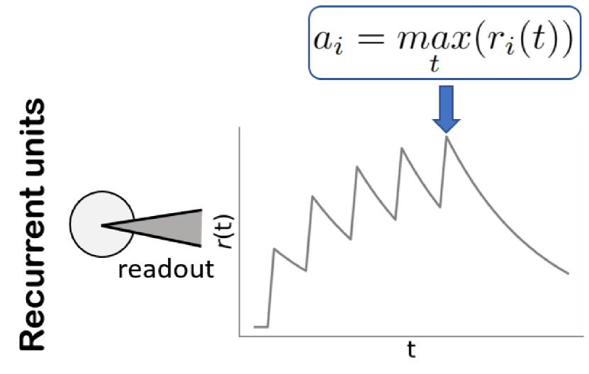
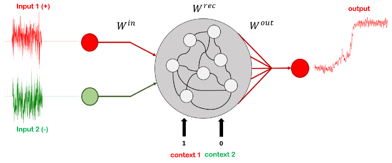
Figure 1: Model structure for MNIST and contextual integration task. (a) Model structure for MNIST task. Each image is converted to spiking activity input to the recurrent reservoir, by Poisson spiking neurons whose rate is determined by the pixel intensity (see details in the main text). $T=100{\rm{ms}}$ in our learning setting. (b) The activity profile of one readout unit for the MNIST task. Only the maximal value is taken for classification. (c) Model structure for contextual integration task. If the cued (context 1 or context 2) input signal is generated using a positive offset value, then the network is supervised to produce an output approaching $+1$ regardless of the irrelevant input signals (e.g., those coming from the other context).

V Experiments using surrogate gradient descents

Throughout our experiments, the Heaviside step function is approximated by a sigmoid surrogate

$$\Theta(x)\approx\frac{x}{1+k|x|},$$ (6)

where a steepness parameter $k$ = 25. Other parameters include $\Delta t=2{\rm{ms}}$, $\tau_{\rm mem}=20{\rm{ms}}$, $\tau_{\rm syn}=10{\rm{ms}}$, $\tau_{d}=30{\rm{ms}}$, $\tau_{r}=2{\rm{ms}}$ and the refractory period $t_{\rm ref}=10{\rm{ms}}$ for all tasks. Because we have not imposed sparsity constraint on the connectivity, we take the initialization scheme that $[\bm{\xi}^{\rm in}\bm{\Sigma}(\bm{\xi}^{\rm out})^{\top}]_{ij}\sim O(\frac{1}{\sqrt{N}})$, similar to what is done in multi-layered perceptron learning [22]. The training is implemented by the adaptive moment estimation (Adam [28]) stochastic gradient descent algorithm to minimize the loss function (cross-entropy for classification or mean-squared error for regression) with a learning rate of $0.001$. We remark that training in the mode space can be done by using automate differentiation on PyTorch. However, we leave the detailed derivation of the learning rule to the supplemental material. Codes are available in our GitHub [29].

V.1 MNIST classification task

As a proof of concept, we apply first SMNN to the benchmark MNIST dataset. The maximum of recurrent unit activity over time is estimated by $a_{i}=\operatorname{max}\limits_{t}(r_{i}(t))$, which are read out by the readout neurons as follows,

$$\mathbf{o}={\operatorname{softmax}}(\bm{W}^{\rm out}\mathbf{a}),$$ (7)

where readout weights $\bm{W}^{\rm out}\in\mathbb{R}^{10\times N}$. Using BPTT, the gradients in the mode space $\bm{\theta}=(\bm{\xi}^{\rm in},\bm{\Sigma},\bm{\xi}^{\rm out})$ is given by

$$\frac{\partial\mathcal{L}}{\partial\bm{\xi}^{\rm in}} =\sum_{t=1}^{T}\frac{\partial\mathcal{L}}{\partial\mathbf{I}(t)}\frac{\partial\mathbf{I}(t)}{\partial\bm{W}^{\rm rec}}\frac{\partial\bm{W}^{\rm rec}}{\partial\bm{\xi}^{\rm in}}=\sum_{t=1}^{T}\frac{\partial\mathcal{L}}{\partial\mathbf{I}(t)}\mathbf{r}(t-1)\bm{\xi}^{\rm out}\bm{\Sigma},$$ (8)

$$\frac{\partial\mathcal{L}}{\partial\lambda_{\mu}} =\sum_{t=1}^{T}\frac{\partial\mathcal{L}}{\partial\mathbf{I}(t)}\frac{\partial\mathbf{I}(t)}{\partial\bm{W}^{\rm rec}}\frac{\partial\bm{W}^{\rm rec}}{\partial\lambda_{\mu}}=\sum_{t=1}^{T}\frac{\partial\mathcal{L}}{\partial\mathbf{I}(t)}\mathbf{r}(t-1)\bm{\xi}^{\rm in}_{\mu}(\bm{\xi}^{\rm out}_{\mu})^{\top},$$

$$\frac{\partial\mathcal{L}}{\partial\bm{\xi}^{\rm out}} =\sum_{t=1}^{T}\frac{\partial\mathcal{L}}{\partial\mathbf{I}(t)}\frac{\partial\mathbf{I}(t)}{\partial\bm{W}^{\rm rec}}\frac{\partial\bm{W}^{\rm rec}}{\partial\bm{\xi}^{\rm out}}=\sum_{t=1}^{T}\frac{\partial\mathcal{L}}{\partial\mathbf{I}(t)}\mathbf{r}(t-1)\bm{\xi}^{\rm in}\bm{\Sigma},$$

where $\bm{\xi}_{\mu}^{\rm in/out}\in\mathbb{R}^{N}$, $T$ is the length of the training trajectory, $\mathcal{L}$ is the loss function, whose gradients $\frac{\partial\mathcal{L}}{\partial\mathbf{I}(t)}$ with respect to total synaptic currents are calculated explicitly in the supplemental material. Each training mini-batch contains $100$ images, and LIF networks with different mode sizes ($P=1,2,\ldots 50,100$) are trained.

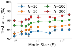
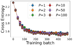
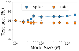
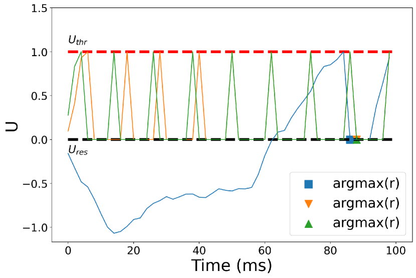
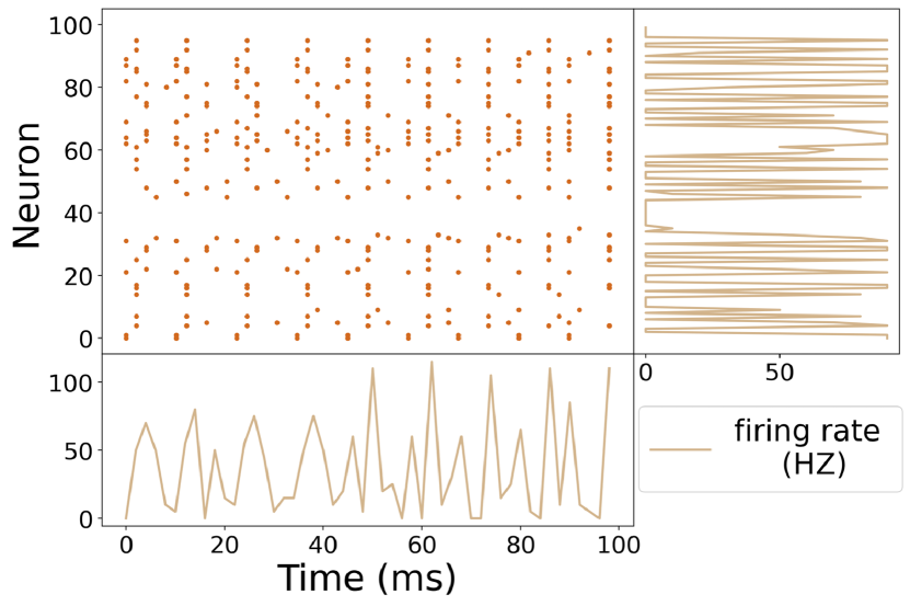
Figure 2: Learning performance of MNIST classification task. Five independent runs are used to estimate the standard deviation. (a) Test accuracy versus different mode size. (b) Loss function as a function of training mini-batch, each composed of $100$ digit images. The mode size varies, and the network size $N=100$. (c) Comparison of the accuracy between rate and spiking model with fixed network size $N$=200. (d) Membrane potential trace for three typical reservoir neurons in response to spike train inputs. The un-smooth profile is due to the discretization of the dynamics with step size $\Delta t$. The triangle marks when the filtered spike train takes a maximum value. $(P,N)=(3,100)$. (e) Spike trains of reservoir neurons with neuron firing rate (right) and population average firing rate (bottom). $(P,N)=(3,100)$.

With increasing mode size, the test accuracy increases [Figure 2 (a) and (b)]. A better generalization is achieved by a larger neural pool. Surprisingly, even for the smallest mode size ($P=1$), the network could be trained to perform well, reaching an accuracy of $96\%$ for $N=200$. In comparison with the rate network counterpart, the spiking model performs better when the mode size is relatively large [Figure 2 (c)], but is more energetic efficient than the rate network. We also plot the membrane potential profile for a few representative neurons, and observe a network synchronous oscillation at a later training stage [Figure 2 (d) and (e)], which signals a neural correlate of visual input classification in neural circuits based on spiking population codes.

V.2 Contextual integration task

In the contextual integration task, the network activity is read out by an affine transformation as

$$o(t)=\bm{W}^{\rm out}\mathbf{r}(t),$$ (9)

where $\bm{W}^{\rm out}\in\mathbb{R}^{1\times N}$ refers to the readout weights, and $\mathbf{r}(t)$ is the filtered spike train. We use the root mean squared (RMSE) loss function defined as

$$\mathcal{L}=\sqrt{\sum_{t=0}^{T}(z(t)-o(t))^{2}},$$ (10)

where $z(t)$ is the target output in time $t$, taking zero except in the response period, and $T$ denotes the time range. In analogy to the previous MNIST classification task, the gradient in the mode space $\bm{\theta}=(\bm{\xi}^{\rm in},\bm{\Sigma},\bm{\xi}^{\rm out})$ for the current context-dependent computation could be similarly derived (see details in the supplemental material). The learning rate was set to $0.001$, and each training mini-batch contains $100$ trials.

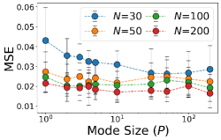
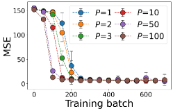
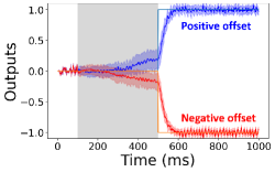
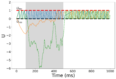
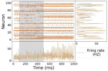
Figure 3: Learning performance of contextual integration task. Five independent runs are used to estimate the standard deviation. (a) Mean squared error (MSE) versus different mode size. (b) MSE as a function of training mini-batch for different mode sizes. The network size $N$=100. (c) Average output activity in response to test inputs for $(P,N)=(3,100)$. The shaded region indicates the stimulus period. Sensory inputs are only shown during the stimulus period, followed by a response period. The fluctuation over $100$ random trials is also shown. Colored lines are two target outputs. (d) Membrane potential trace for four typical reservoir neurons in response to a random input. The shaded region indicates the stimulus period. (e) Spike raster of reservoir neurons with neuron firing rate (right) and population average firing rate (bottom). $(P,N)=(3,100)$ for (d) and (e).

As shown in Figure 3 (a), the test MSE does not vary strongly with the mode size, especially for a relatively large neural population. For a smaller one $N=30$, the performance becomes better with increasing the value of $P$. However, the best performance is still worse than that of large-sized networks. The training dynamics in Figure 3 (b) shows that a larger value of $P$ speeds up the learning. Figure 3 (c) confirms that our training protocol succeeds in reproducing the result of Monkey’s experiments on the task of flexible selective integration of sensory inputs. We can even look at the dynamics profile of the membrane potential. During the stimulus period, each neuron has its own time scales to encode the input signals, and at a network scale, we do not observe any regular patterns. However, after the sensory input is turned off, the network is immediately required to make a decision, and we observe that the firing frequency of the neural pool is elevated, and interestingly, some neurons seem to keep the same pace. This will reflect basic properties of neural manifold behind the perceptual decision making, which we shall detail in the next section.

V.3 Projection in the mode space

To study the neural manifold underlying the perceptual decision making, we project the high dimensional neural activity onto the mode space. If the small number of modes is sufficient to capture the performance, we can visualize the manifold without using the principal component analysis that is impossible to keep all information in a low dimensional space in general. This is one merit of our method. As expected, after training, four separated attractors are formed in the mode space, either in the input mode space or in the output mode space [Figure 4 (a)]. The test dynamics would flow to the corresponding attractor depending on the context of the task.

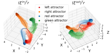
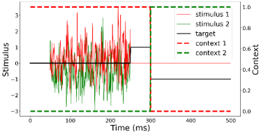
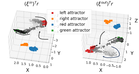
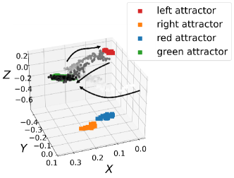
Figure 4: The filtered spike train of hidden layer projected to the mode space for the contextual integration task. The mode size $P=3$, and the network size $N=100$. (a) Projection into the input mode space. Three hundred randomly generated trials were used. Different colors encode different offset sign and contextual cue. The color gets darker with time in the dynamics trajectory. (b) Context switching experiment. At $t=300\rm{ms}$, the previous contextual cue is shifted to the other one. The left-y axis encodes the input signals, while the right-y axis encodes the contextual information. (c) Activity projection for the context switching experiment in (b). (d) Projection coefficient in the input mode space for the context switching experiment in (b).

We next consider a context switching experiment, and look at how the dynamics is changed in the low dimensional intrinsic space. The experimental protocol is shown in Figure 4 (b). At $t=300\rm{ms}$, the context is switched to the other one, and the network should carry out computation according to the new context, e.g., making a correct response to the input signal. Before the context is switched, the context cued input signals have a positive offset. Correspondingly, the neural activity trajectory in the mode space evolves to the left attractor [Figure 4 (c)]. Once the context is switched, the context cues another input signal that has a negative offset. The neural trajectory is then directed to the neighboring green attractor. Therefore, the neural dynamics can be guided by the contextual cue, mimicking what occurs in the prefrontal cortex of Monkeys that perform the contextual integration task [23].

V.4 Power law for connectivity importance scores

We next find whether some modes are more important than the others. To make comparable the magnitudes of the pattern and importance scores, we rank the modes according to the following measure [22]

$$\tau_{\mu}=\chi||\bm{\xi}^{\rm in}_{\mu}||_{2}+\chi||\bm{\xi}^{\rm out}_{\mu}||_{2}+|\lambda_{\mu}|,$$ (11)

where $\bm{\xi}_{\mu}^{\rm{in}/\rm{out}}\in\mathbb{R}^{N}$ $\chi=\sum_{\mu}|\lambda_{\mu}|/\sum_{\mu}(\|\bm{\xi}^{\rm in}_{\mu}\|_{2}+\|\bm{\xi}^{\rm out}_{\mu}\|_{2})$. We observe a piecewise power law for the $\tau$ measure (Figure 5), implying that the ambient space of neural activity is actually low-dimensional, and can be projected to a low dimensional mode space, with $P_{\rm dom}$ (taking a small value in Figure 5) dominant coordinate axes on which the importance scores vary mildly. On one hand, the task information is coded hierarchically into the mode space, and on the other hand, this observation supports that a fast training of spiking networks is possible by focusing on leading modes explaining the network macroscopic behavior.

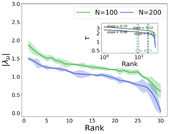
Figure 5: Connectivity importance $|\lambda_{\mu}|$ versus rank (in descending order). The contextual integration task is considered, and the simulation condition is the same with that in Figure 3. We fix $P=30$. Three independent runs are used to estimate the standard deviation. We also define a more precise measure $\tau_{\mu}=\chi\|\bm{\xi}^{\rm in}_{\mu}\|_{2}+\chi\|\bm{\xi}^{\rm out}_{\mu}\|_{2}+|\lambda_{\mu}|$, where $\chi=\sum_{\mu}|\lambda_{\mu}|/\sum_{\mu}(\|\bm{\xi}^{\rm in}_{\mu}\|_{2}+\|\bm{\xi}^{\rm out}_{\mu}\|_{2})$. There appears the piecewise power law behavior in the inset of the log-log plot.

V.5 Reduced dynamics in the mode space

Here, we will show how the dynamics of network activity based on our SMNN learning in the contextual integration task can be projected to a low dimensional counterpart. We follow the previous works of low-rank recurrent neural networks [16, 18]. To construct a subspace spanned by orthogonal bases, we first split $\bm{W}^{\rm in}$ into the parts parallel and orthogonal to the input mode $\bm{\xi}^{\rm in}$,

$$\bm{W}^{\rm in}_{s}=\sum_{\mu}\alpha_{\mu}\bm{\xi}^{\rm in}_{\mu}+\beta_{s}\bm{W}_{\bot}^{s},$$ (12)

where $s$ indicates which component of input signals, $\alpha_{\mu}$ and $\beta_{s}$ are coefficients for the linear combination. We assume that the bases are orthogonal; otherwise, one can use Gram-Schmidt procedure to obtain the orthogonal bases.

We can then express the membrane potential $\mathbf{U}(t)$ in the above orthogonal bases as

$$\mathbf{U}(t)=\sum_{\mu}\gamma_{\mu}(t)\bm{\xi}^{\rm in}_{\mu}+\sum_{s}v_{s}(t)\bm{W}_{\bot}^{s},$$ (13)

where the coefficients for the linear combination are given below,

$$\gamma_{\mu}(t)=\frac{(\bm{\xi}^{\rm in}_{\mu})^{\top}\mathbf{U}(t)}{(\bm{\xi}^{\rm in}_{\mu})^{\top}\bm{\xi}^{\rm in}_{\mu}},$$ (14)

$$v_{s}(t)=\frac{(\bm{W}_{\bot}^{s})^{\top}\mathbf{U}(t)}{(\bm{W}_{\bot}^{s})^{\top}\bm{W}_{\bot}^{s}}.$$

With the above linear combination, the dynamics of $\mathbf{v}(t)$ is captured by

$$\tau_{\rm mem}\frac{{\rm{d}}v_{s}(t)}{{\rm{d}}t}=-v_{s}(t)+\beta_{s}u_{s}(t),$$ (15)

which is derived by using the original dynamics of the membrane potential [Eq. (1)].

Similarly, we obtain the dynamics of $\bm{\gamma}(t)$ as follows,

$$\tau_{\rm mem}\frac{{\rm{d}}\bm{\gamma}(t)}{{\rm{d}}t}=\mathbf{F}(t,\bm{\gamma}(t),\mathbf{r}(t),\mathbf{u}(t)),$$ (16)

where the force function $\bm{F}$ is defined below,

$$\mathbf{F}=-\bm{\gamma}(t)+\bm{\Sigma}(\bm{\xi}^{\rm out})^{\top}\mathbf{r}(t)+\bm{\alpha}\odot\mathbf{b},$$ (17)

where the vector $\mathbf{b}=\sum_{s}u_{s}(t)\mathcal{I}$, and $\mathcal{I}$ is an all-one vector of dimension $P$. To derive Eq. (17), we have made fast synaptic dynamics assumption, i.e., $\tau_{\rm syn}\to 0$. In addition, the filtered spike trains $\mathbf{r}(t)$ can also be written as a form of linear combination,

$$\bm{r}(t)=\sum_{\mu}\kappa_{\mu}(t)\bm{\xi}^{\rm in}_{\mu}+\sum_{s}\nu_{s}(t)\bm{W}_{\bot}^{s},$$ (18)

where the coefficients are given respectively by

$$\kappa_{\mu}(t) =\frac{(\bm{\xi}^{\rm in}_{\mu})^{\top}\mathbf{r}(t)}{(\bm{\xi}^{\rm in}_{\mu})^{\top}\bm{\xi}^{\rm in}_{\mu}},$$ (19)

$$\nu_{s}(t) =\frac{(\bm{W}_{\bot}^{s})^{\top}\mathbf{r}(t)}{(\bm{W}_{\bot}^{s})^{\top}\bm{W}_{\bot}^{s}}.$$

Next, we consider a simple exponential synaptic filter characterized by a time constant $\tau_{s}$ (other synapse types can be similarly analyzed), and project the spiking activity $\mathbf{S}$ onto the orthogonal bases. The resulting reduced dynamics thus reads

$$\tau_{s}\frac{{\rm{d}}\nu_{s}(t)}{{\rm{d}}t}=-\nu_{s}(t)+\frac{(\bm{W}_{\bot}^{s})^{\top}\mathbf{S}(t)}{(\bm{W}_{\bot}^{s})^{\top}\bm{W}_{\bot}^{s}}.$$ (20)

In addition, we also have

$$\tau_{s}\frac{{\rm{d}}\kappa_{\mu}(t)}{{\rm{d}}t}=-\kappa_{\mu}(t)+\frac{(\bm{\xi}^{\rm in}_{\mu})^{T}\mathbf{S}(t)}{(\bm{\xi}^{\rm in}_{\mu})^{\top}\bm{\xi}^{\rm in}_{\mu}}.$$ (21)

The spiking activity is indicated by $\mathbf{S}(t)=\Theta\Bigl{(}\sum_{\mu}\gamma_{\mu}(t)\bm{\xi}^{\rm in}_{\mu}+\sum_{s}v_{s}(t)\bm{W}_{\bot}^{s}-U_{\rm thr}\mathcal{I}\Bigr{)}$. We plot the dynamics of $\bm{\kappa}$ for the context switching experiment [Figure 4(d)], which reveals the qualitatively same behavior as observed in Figure 4 (c).

VI Conclusion

In this work, we propose a spiking mode-based neural network framework for training various computational tasks. This framework is based on mode decomposition learning inspired from Hopfield network and multi-layered perceptron training [20, 22]. From the SMNN learning rule, we can adapt the mode size to the task difficulty, and retrieve the pow-law behavior of the importance scores, and furthermore, the high dimensional recurrent activity can be projected to the low-dimensional mode space with a few leading modes, derived from the pow-law behavior. Using a few modes, we can speed up the training of recurrent spiking networks, thereby making a large scale of spike-based computation possible in practice. Further extension of our work allows us treating more realistic biological networks, e.g., considering excitatory-inhibitory networks, sparsity of network connections, and sequence memory from network activity, etc. To conclude, our work provides a fast, interpretable and biological plausible framework for analyzing the neuroscience experiments and designing brain-like computation circuits.

VII Acknowledgments

We thank Yang Zhao for an earlier involvement of this project, especially the derivation of the discretization of continuous neural and synaptic dynamics, and Yuhao Li for helpful discussions. This research was supported by the National Natural Science Foundation of China for Grant Number 12122515 (H.H.), and Guangdong Provincial Key Laboratory of Magnetoelectric Physics and Devices (No. 2022B1212010008), and Guangdong Basic and Applied Basic Research Foundation (Grant No. 2023B1515040023).

Appendix A Discretization of continuous neural and synaptic dynamics

The interested continuous dynamics can be written in the following form,

$$\tau\frac{\mathrm{d}x}{\mathrm{d}t}=-x(t)+y(t),$$ (22)

where $y(t)$ is a time-dependent driving term. This first-order linear differential equation has a solution,

$$x(t)=\frac{1}{\tau}e^{-t/\tau}\int_{0}^{t}y(s)e^{s/\tau}ds,$$ (23)

which implies that $x(0)=0$. Next, we assume the discretization step size $\Delta t$ is a small quantity. We then have

$$\begin{split}x(t+\Delta t)&=\frac{1}{\tau}e^{-\frac{t+\Delta t}{\tau}}\int_{0}^{t+\Delta t}y(s)e^{s/\tau}ds\\ &=\lambda_{\tau}x(t)+\frac{1}{\tau}e^{-\frac{t+\Delta t}{\tau}}\int_{t}^{t+\Delta t}y(s)e^{s/\tau}ds\\ &=\lambda_{\tau}x(t)+\frac{\lambda_{\tau}}{\tau}\int_{0}^{\Delta t}y(t+s)e^{s/\tau}ds\\ &\simeq\lambda_{\tau}x(t)+\frac{\lambda_{\tau}}{\tau}y(t)\int_{0}^{\Delta t}e^{s/\tau}ds\\ &=\lambda_{\tau}x(t)+(1-\lambda_{\tau})y(t),\end{split}$$ (24)

where we change the integral variable in the third equality, and the approximation in the fourth line holds when $\Delta t$ is close to zero, and we define $\lambda_{\tau}=e^{-\Delta t/\tau}$. Note that in our simulations, $\tau_{r}$ and $\tau_{\rm syn}$ are relatively small, and therefore we neglect the corresponding decay factor in the second term of the last line in Eq. (24). A full set of discrete dynamics is given in Eq. (25).

Appendix B Derivation of mode-based learning rules

In this section, we provide details to derive the spiking mode-based learning rules. First, the discrete update rules for the dynamics are given below,

$$\mathbf{r}(t+1) =\lambda_{d}\mathbf{r}(t)+(1-\lambda_{d})\mathbf{h}(t+1),$$ (25)

$$\mathbf{h}(t+1) =\lambda_{r}\mathbf{h}(t)+\mathbf{S}(t+1),$$

$$\mathbf{U}(t+1) =\Big{(}\lambda_{\rm mem}\mathbf{U}(t)+(1-\lambda_{\rm mem})\mathbf{I}(t+1))\Big{)}\odot\Big{(}\mathcal{I}-\mathbf{S}(t)\Big{)},$$

$$\mathbf{I}(t+1) =\lambda_{\rm syn}\mathbf{I}(t)+\bm{W}^{\rm rec}\mathbf{r}(t)+\bm{W}^{\rm in}\mathbf{u}(t),$$

where $t$ is a discrete time step (or in the unit of $\Delta t$), and $\lambda_{i}=\exp{(-\Delta t/\tau_{i})}$. With the loss function $\mathcal{L}$, we define the following error gradients $\bm{\mathcal{K}}(t)\equiv\frac{\partial\mathcal{L}}{\partial\mathbf{r}(t)}$, and by using the chain rule, we immediately have the following results.

case 1

$t=T$:

$$\frac{\partial\mathcal{L}}{\partial\mathbf{r}(T)} =\bm{\mathcal{K}}(T),$$ (26)

$$\frac{\partial\mathcal{L}}{\partial\mathbf{I}(T)} =\bm{\mathcal{K}}(T)\frac{\partial\mathbf{r}(T)}{\partial\mathbf{I}(T)}.$$

case 2

$t<T$:

$$\frac{\partial\mathcal{L}}{\partial\mathbf{r}(t)} =\bm{\mathcal{G}}(t)+\bm{\mathcal{K}}(t+1)\frac{\partial r(t+1)}{\partial\mathbf{r}(t)}$$ (27)

$$=\bm{\mathcal{G}}(t)+\lambda_{d}\bm{\mathcal{K}}(t+1),$$

$$\frac{\partial\mathcal{L}}{\partial\mathbf{I}(t)} =\frac{\partial\mathcal{L}}{\partial\mathbf{I}(t+1)}\frac{\partial\mathbf{I}(t+1)}{\partial\mathbf{I}(t)}+\frac{\partial\mathcal{L}}{\partial\mathbf{r}(t)}\frac{\partial\mathbf{r}(t)}{\partial\mathbf{I}(t)}$$

$$=\lambda_{\rm syn}\bm{\mathcal{K}}(t+1)\frac{\partial\mathbf{r}(t+1)}{\partial\mathbf{I}(t+1)}+\bm{\mathcal{K}}(t)\frac{\partial\mathbf{r}(t)}{\partial\mathbf{I}(t)},$$

where $\bm{\mathcal{G}}(t)$ is the explicit differentiation of $\mathcal{L}$ with respect to $\mathbf{r}(t)$. Using the surrogate gradient of the step function, we have

$$\mathbf{S}(t) =\Theta(\mathbf{U}(t)-U_{\rm thr}\mathcal{I})\approx\frac{\mathbf{U}(t)-U_{\rm thr}\mathcal{I}}{1+k|\mathbf{U}(t)-U_{\rm thr}\mathcal{I}|},$$ (28)

$$\frac{\partial\mathbf{S}(t)}{\partial\mathbf{U}(t)} ={\operatorname{diag}}\Big{(}\frac{1}{(1+k|\mathbf{U}(t)-U_{\rm thr}\mathcal{I}|)^{2}}\Big{)},$$

where $\mathcal{I}$ represents an all-one vector, and $|\mathbf{a}|$ for a vector $\mathbf{a}$ equals to $|a_{i}|$ when the $i$-th component is considered. As a result, we can easily get

$$\frac{\partial\mathbf{r}(t)}{\partial\mathbf{I}(t)} =\frac{\partial\mathbf{r}(t)}{\partial\mathbf{h}(t)}\frac{\partial\mathbf{h}(t)}{\partial\mathbf{S}(t)}\frac{\partial\mathbf{S}(t)}{\partial\mathbf{U}(t)}\frac{\partial\mathbf{U}(t)}{\partial\mathbf{I}(t)}$$ (29)

$$=(1-\lambda_{d})(1-\lambda_{\rm mem}){\operatorname{diag}}\Big{(}\frac{1}{(1+k|\mathbf{U}(t)-U_{\rm thr}\mathcal{I}|)^{2}}\Big{)}.$$

Therefore, we can update the mode component and the connectivity importance as follows,

$$\frac{\partial\mathcal{L}}{\partial\bm{\xi}^{\rm in}} =\sum_{t=1}^{T}\frac{\partial\mathcal{L}}{\partial\mathbf{I}(t)}\frac{\partial\mathbf{I}(t)}{\partial\bm{W}^{\rm rec}}\frac{\partial\bm{W}^{\rm rec}}{\partial\bm{\xi}^{\rm in}}=\sum_{t=1}^{T}\frac{\partial\mathcal{L}}{\partial\mathbf{I}(t)}\mathbf{r}(t-1)\bm{\xi}^{\rm out}\bm{\Sigma},$$ (30)

$$\frac{\partial\mathcal{L}}{\partial\lambda_{\mu}} =\sum_{t=1}^{T}\frac{\partial\mathcal{L}}{\partial\mathbf{I}(t)}\frac{\partial\mathbf{I}(t)}{\partial\bm{W}^{\rm rec}}\frac{\partial\bm{W}^{\rm rec}}{\partial\lambda_{\mu}}=\sum_{t=1}^{T}\frac{\partial\mathcal{L}}{\partial\mathbf{I}(t)}\mathbf{r}(t-1)\bm{\xi}^{\rm in}_{\mu}(\bm{\xi}^{\rm out}_{\mu})^{\top},$$

$$\frac{\partial\mathcal{L}}{\partial\bm{\xi}^{\rm out}} =\sum_{t=1}^{T}\frac{\partial\mathcal{L}}{\partial\mathbf{I}(t)}\frac{\partial\mathbf{I}(t)}{\partial\bm{W}^{\rm rec}}\frac{\partial\bm{W}^{\rm rec}}{\partial\bm{\xi}^{\rm out}}=\sum_{t=1}^{T}\frac{\partial\mathcal{L}}{\partial\mathbf{I}(t)}\mathbf{r}(t-1)\bm{\xi}^{\rm in}\bm{\Sigma}.$$

For the handwritten digit classification task, $a_{i}=\mathop{max}\limits_{t}(r_{i}(t))=r_{i}(t_{i}^{m}),\mathbf{o}={\rm{softmax}}(\bm{W}^{\rm out}\mathbf{a})$ and $\mathcal{L}=-\mathbf{z}^{T}\ln\mathbf{o}$, where $t_{i}^{m}$ is the time when the maximal firing rate is reached, and $\mathbf{z}$ is the one-hot target label. We then have the following equations for updating time-dependent error gradients.

$$\mathcal{K}_{i}(T) =\frac{\partial\mathcal{L}}{\partial a_{i}}\sum_{j}\frac{\partial a_{i}}{\partial r_{j}(T)}$$ (31)

$$=\Big{(}(\mathbf{o}-\mathbf{z})\bm{W}^{\rm out}\Big{)}_{i}\sum_{j}\frac{\partial r_{i}(t_{i}^{m})}{\partial r_{j}(T)}$$

$$=\Big{(}(\mathbf{o}-\mathbf{z})\bm{W}^{\rm out}\Big{)}_{i}\sum_{j}\frac{\partial r_{i}(t_{i}^{m})}{\partial r_{j}(t_{i}^{m})}\delta(T-t_{i}^{m})$$

$$=\Big{(}(\mathbf{o}-\mathbf{z})\bm{W}^{\rm out}\Big{)}_{i}\delta(T-t_{i}^{m}),$$

and

$$\mathcal{K}_{i}(t) =\frac{\partial\mathcal{L}}{\partial a_{i}}\sum_{j}\frac{\partial a_{i}}{\partial r_{j}(t)}+\lambda_{d}\mathcal{K}_{i}(t+1)$$ (32)

$$=\Big{(}((\mathbf{o}-\mathbf{z})\bm{W}^{\rm out}\Big{)}_{i}\sum_{j}\frac{\partial a_{i}}{\partial r_{j}(t)}+\lambda_{d}\mathcal{K}_{i}(t+1),\forall t<T.$$

The sum in the first term of the last equality in Eq. (32) can be explicitly calculated out, i.e.,

$$\sum_{j}\frac{\partial a_{i}}{\partial r_{j}(t)} =\sum_{j}\frac{\partial r_{i}(t_{i}^{m})}{\partial r_{j}(t)}$$ (33)

$$=\sum_{j}\frac{\partial r_{i}(t_{i}^{m})}{\partial r_{j}(t_{i}^{m})}\delta(t-t_{i}^{m})+\sum_{j}\frac{\partial r_{i}(t_{i}^{m})}{\partial r_{j}(t_{i}^{m}-1)}\delta(t+1-t_{i}^{m})$$

$$=\delta(t+1-t_{i}^{m})\sum_{j}\Big{[}\delta_{ij}\lambda_{d}+\left[\frac{\partial\mathbf{r}(t_{i}^{m})}{\partial\mathbf{I}(t_{i}^{m})}\right]_{ii}\Big{(}W^{\rm rec}_{ij}+\lambda_{\rm syn}\left[\frac{\partial\mathbf{I}(t_{i}^{m}-1)}{\partial\mathbf{r}(t_{i}^{m}-1)}\right]_{ij}\Big{)}\Big{]}+\delta(t-t_{i}^{m}),$$

where the term $\left[\frac{\partial\mathbf{I}(t_{i}^{m}-1)}{\partial\mathbf{r}(t_{i}^{m}-1)}\right]_{ij}=0$ for $i\neq j$ [Eq. (29)].

For the contextual integration task, $o(t)=\bm{W}^{\rm out}\mathbf{r}$ and $\mathcal{L}=\sqrt{\sum_{t=0}^{T}(z(t)-o(t))^{2}}$, where $z(t)$ is the target output. In a similar way, one can derive the following error gradients,

$$\bm{\mathcal{K}}(T) =\frac{z(T)-o(T)}{\mathcal{L}}\bm{W}^{\rm out},$$ (34a)

$$\bm{\mathcal{K}}(t) =\frac{z(t)-o(t)}{\mathcal{L}}\bm{W}^{\rm out}+\lambda_{d}\bm{\mathcal{K}}(t+1),\forall t<T.$$ (34b)

The other update equations are the same as above.

Appendix C Initialization and model parameters

The initialization scheme is given in Table 2, where the constructed recurrent weights should be multiplied by a factor of $\frac{1}{\sqrt{PN}}$ [22]. The hyper parameters used in the neural dynamics equations are given in Table 3.

Table 2: Parameter initialization

Parameter	Initial distribution	Description
$\bm{W}^{\rm in}$	$\mathcal{N}(0,1/N_{\rm in})$	Input weight
$\bm{\xi}^{\rm in}$	$\mathcal{N}(0,1)$	Input mode
$\bm{\xi}^{\rm out}$	$\mathcal{N}(0,1)$	Output mode
$\lambda_{\mu}$	$\mathcal{N}(0,1)$	Connectivity importance
$\bm{W}^{\rm out}$	$\mathcal{N}(0,1/N)$	Readout weight

Table 3: Model parameters

Parameter	Value	Description
$\Delta t$	2ms	Discretization step size
$\tau_{\rm mem}$	20ms	Membrane time constant
$\tau_{\rm syn}$	10ms	Synaptic time constant
$\tau_{r}$	2ms	Synaptic rise time
$\tau_{d}$	30ms	Synaptic decay time
$t_{\rm ref}$	10ms	Refractory period
$k$	25	Steepness parameter

References

- [1] Wulfram Gerstner, Werner M. Kistler, Richard Naud, and Liam Paninski. Neuronal Dynamics: From Single Neurons to Networks and Models of Cognition. Cambridge University Press, United Kingdom, 2014.
- [2] Kaushik Roy, Akhilesh Jaiswal, and Priyadarshini Panda. Towards spike-based machine intelligence with neuromorphic computing. Nature, 575(7784):607–617, 2019.
- [3] Paul J. Werbos. Backpropagation through time: What it does and how to do it. Proc. IEEE, 78:1550–1560, 1990.
- [4] Jeffrey L. Elman. Finding structure in time. Cognitive Science, 14(2):179–211, 1990.
- [5] Haiping Huang. Statistical Mechanics of Neural Networks. Springer, Singapore, 2022.
- [6] Mehrdad Jazayeri and Srdjan Ostojic. Interpreting neural computations by examining intrinsic and embedding dimensionality of neural activity. Current Opinion in Neurobiology, 70:113–120, 2021.
- [7] Emre O. Neftci, Hesham Mostafa, and Friedemann Zenke. Surrogate gradient learning in spiking neural networks: Bringing the power of gradient-based optimization to spiking neural networks. IEEE Signal Processing Magazine, 36(6):51–63, 2019.
- [8] Julian Rossbroich, Julia Gygax, and Friedemann Zenke. Fluctuation-driven initialization for spiking neural network training. Neuromorphic Computing and Engineering, 2(4):044016, 2022.
- [9] David Sussillo and Larry F Abbott. Generating coherent patterns of activity from chaotic neural networks. Neuron, 63(4):544–557, 2009.
- [10] Dominik Thalmeier, Marvin Uhlmann, Hilbert J Kappen, and Raoul-Martin Memmesheimer. Learning universal computations with spikes. PLoS computational biology, 12(6):e1004895, 2016.
- [11] Wilten Nicola and Claudia Clopath. Supervised learning in spiking neural networks with force training. Nature communications, 8(1):2208, 2017.
- [12] Christopher M Kim and Carson C Chow. Learning recurrent dynamics in spiking networks. Elife, 7:e37124, 2018.
- [13] Robert Kim, Yinghao Li, and Terrence J Sejnowski. Simple framework for constructing functional spiking recurrent neural networks. Proceedings of the national academy of sciences, 116(45):22811–22820, 2019.
- [14] Brian DePasquale, Mark M Churchland, and LF Abbott. Using firing-rate dynamics to train recurrent networks of spiking model neurons. arXiv:1601.07620, 2016.
- [15] Larry F Abbott, Brian DePasquale, and Raoul-Martin Memmesheimer. Building functional networks of spiking model neurons. Nature neuroscience, 19(3):350–355, 2016.
- [16] Francesca Mastrogiuseppe and Srdjan Ostojic. Linking connectivity, dynamics, and computations in low-rank recurrent neural networks. Neuron, 99(3):609–623, 2018.
- [17] Manuel Beiran, Nicolas Meirhaeghe, Hansem Sohn, Mehrdad Jazayeri, and Srdjan Ostojic. Parametric control of flexible timing through low-dimensional neural manifolds. Neuron, 111(5):739–753, 2023.
- [18] Ljubica Cimesa, Lazar Ciric, and Srdjan Ostojic. Geometry of population activity in spiking networks with low-rank structure. PLOS Computational Biology, 19(8):1–34, 2023.
- [19] William F. Podlaski and Christian K. Machens. Approximating nonlinear functions with latent boundaries in low-rank excitatory-inhibitory spiking networks. arXiv:2307.09334, 2023.
- [20] Zijian Jiang, Jianwen Zhou, Tianqi Hou, K. Y. Michael Wong, and Haiping Huang. Associative memory model with arbitrary hebbian length. Phys. Rev. E, 104:064306, 2021.
- [21] Zijian Jiang, Ziming Chen, Tianqi Hou, and Haiping Huang. Spectrum of non-hermitian deep-hebbian neural networks. Phys. Rev. Res., 5:013090, 2023.
- [22] Chan Li and Haiping Huang. Emergence of hierarchical modes from deep learning. Phys. Rev. Res., 5:L022011, 2023.
- [23] Valerio Mante, David Sussillo, Krishna V Shenoy, and William T Newsome. Context-dependent computation by recurrent dynamics in prefrontal cortex. Nature, 503(7474):78–84, 2013.
- [24] H Francis Song, Guangyu R Yang, and Xiao-Jing Wang. Training excitatory-inhibitory recurrent neural networks for cognitive tasks: a simple and flexible framework. PLoS computational biology, 12(2):e1004792, 2016.
- [25] Benjamin Cramer, Yannik Stradmann, Johannes Schemmel, and Friedemann Zenke. The heidelberg spiking data sets for the systematic evaluation of spiking neural networks. IEEE Transactions on Neural Networks and Learning Systems, 33(7):2744–2757, 2022.
- [26] Yann LeCun. The MNIST database of handwritten digits, retrieved from http://yann.lecun.com/exdb/mnist., 1998.
- [27] Thomas Miconi. Biologically plausible learning in recurrent neural networks reproduces neural dynamics observed during cognitive tasks. Elife, 6:e20899, 2017.
- [28] Diederik P. Kingma and Jimmy Ba. Adam: A method for stochastic optimization. arXiv:1412.6980, 2014.
- [29] Zhanghan Lin and Haiping Huang. https://github.com/LinZhanghan/SMNN, 2023.