Adversarial Training for Physics-Informed Neural Networks

Abstract

Physics-informed neural networks (PINNs) have shown great promise in solving partial differential equations (PDEs). However, due to insufficient robustness, vanilla PINNs often face challenges when solving complex PDEs, especially those involving multi-scale behaviors or solutions with sharp or oscillatory characteristics. To address these issues, based on the projected gradient descent (PGD) adversarial attack, we proposed an adversarial training strategy for PINNs termed by AT-PINNs. AT- PINNs enhance the robustness of PINNs by fine-tuning the model with adversarial samples, which can accurately identify model failure locations and drive the model to focus on those regions during training. AT-PINNs can also perform inference with temporal causality by selecting the initial collocation points around temporal initial values. We implement AT-PINNs to the elliptic equation with multi-scale coefficients, Poisson equation with multi-peak solutions, Burgers’ equation with sharp solutions and the Allen–Cahn equation. The results demonstrate that AT-PINNs can effectively locate and reduce failure regions. Moreover, AT-PINNs are suitable for solving complex PDEs, since locating failure regions through adversarial attacks is independent of the size of failure regions or the complexity of the distribution.

An adversarial attack based sampling and training scheme (AT-PINN) is proposed to refine PINNs on failure regions, which is especially effective in solving challenging problems encountered by PINNs, including multi-scale behavior, sharp or oscillatory solutions, and temporal causality problems, etc.

An adversarial attack method (PINN-PGD) is proposed to generate adversarial samples for PINNs, which adaptively capture local maximums of the model residual as failure regions. The adversarial attack can adaptively locate failure regions despite of the volume of the failure region, the dimension of the problem and the distribution hypothesis of the residual map.

The effectiveness of AT-PINN is verified on the elliptic equation with multi-scale coefficients, Poisson equation with multi-peak solutions, Burgers’ equation with sharp solutions, and the Allen–Cahn equation.

1 Introduction

Physics-informed neural networks (PINNs) are a type of model-data hybrid-driven methods for solving partial differential equations (PDEs). They combine physical laws and data measurements into the loss function and utilize automatic differentiation to drive the learning process [1]. PINNs enjoy plenty of advantages such as : (i) mesh-free, which enables PINNs the potential of solving complex domain problems and high dimension problems; (ii) the flexibility to impose physical constrains and data information; (iii) the ability to handle nonlinear problems, which is supported by the universal approximation theorem and the variety of activation functions. Therefore, PINNs have been shown as new promising paradigms for solving PDEs (forward problems) and estimating model parameters (inverse problems) in a wide range of physic phenomena and applications, see for instance, solving Euler equations with high speed flows [2], Navier-Stokes equations [3], phase-field equations [4], characterizing parameters in biology systems [5] and fluid dynamics [6], etc. They also gain increasing attention in areas such as fractional equations [7], integro-differential equations [8] and stochastic PDEs [9].

Despite fruitful results have been obtained, vanilla PINNs face challenges when solving more complicated problems. To improve the performance, numerous variants have been proposed based on the structure of neural networks and the property of the PDEs. Some notable works include PINNs with new differentiation methods like CAN-PINN [10], hybird-PINN [11], new activation functions with adaptable hyper-parameters based on scaling factor [12], and various temporal discretization methods like parareal PINN[13], bc-PINN [4], causal-PINN [14]. New loss designs such as gPINNs[15] and new formulations based on Galerkin methods like VPINNs[16], hp-PINNs[17] . For a more comprehensive understanding of PINNs and their variants, we refer to the review paper [18, 19, 20].

While benefiting from the advantages of learning mechanisms, PINNs also suffer the inherent limitations of deep neural networks. One of the most doubtful aspect is their robustness, i.e., a small perturbation on the input sample may lead to neural network misclassification or regression failure [21]. Therefore, attackers can attack the neural networks by intentionally manipulates the input data and cause the model to produce incorrect outputs. This type of attack is called adversarial attack and such samples that fail the neural network are called adversarial samples. It has been studied that neural networks are generally not robust and are particularly vulnerable to adversarial attacks [22], and the neural network based PINNs are not an exception. Especially, in the framework of vanilla PINNs, the learning process is driven by minimize the PDE residual at a pre-selected set of training samples. It is challenge to guarantee the accuracy of the model on the whole domain. Luckily, by identifying adversarial samples of a PINN, one can locate where the PINN has inaccurate approximation. Thus, one can further using adversarial samples to improve the model performance [23].

In this paper, we propose to refine PINNs with adversarial training (AT-PINN), which fine-trains the model by adaptively adding new adversarial samples to improve model performance. Adversarial training is one of the most effective method to improve the robustness of neural networks [24] and has been widely used in large neural language models for performance boosting [25]. For PINNs, adversarial samples can automatically and accurately adapt to the model failure locations and force the model to focus on the failure regions during the adversarial training. The failure location adaptation is independent from the volume of the failure region, the dimension of the problem or the distribution of the residual map, which is especially helpful in solving PDEs with specific characteristics such as multi-scale behavior, sharp or oscillatory solutions, temporal causality, etc.

1.1 Related Works and Contributions

Adversarial training can be related to sampling strategies of PINNs as it enhancing PINNs through specially designed sampling. In the vanilla PINN algorithm, since PINNs are supposed to approximate the equation solution on the entire problem domain, Latin hypercube sampling (LHS) and uniform sampling are proposed to generate training samples [1], which generally perform well for a wide range of cases, but may fail in solving more complex PDEs.

The un-biased sampling face challenges when the PDEs involving some irregular features such as multi-scale behavior, sharp or oscillatory solutions. To overcome these issues, various residual-based adaptive sampling methods have been proposed to improve the performance of PINNs. Lu et al. [18] first proposed a residual-based adaptive refinement (RAR) method, which repeatedly adds new collocation points at where the PDE residual is large. Mao et al. [26] further divided the whole domain into several sub-domain and presented the adaptive sampling methods (ASMs) based on both the mean value of the residual for each sub-domain and the gradient of the solution. ASMs can eliminate the occasionally of bad residual points and resulting in a more stable iteration procedure. Different from RAR and ASMs, Wu et al. [27] resample new collocations by constructing a new probability density function with two hyper parameters based on the PDE residual. Another attractive work from the point view of probability density is the failure-informed PINNs (FI-PINNs), which use an effective failure probability based on the residual as the posterior error indicator to place more collocation points in the failure region [28]. Two extensions of FI-PINN based on re-sampling technique and subset simulation algorithm were consequently established in [29].

Residual-based sampling strategies and AT-PINN both aim to improve the performance of PINNs by adaptively adding new samples where the model fails and retraining on them. However, they differ in the way they search for these new samples. In the residual based methods, the high-residual region searchings are implemented through Monte Carlo sampling (e.g. RAR), brute force searching (e.g. ASMs), residual distribution approximating (e.g. FI-PINN), etc. Their effectiveness depend on the volume of the failure region, the dimension of the problem and the distribution hypothesis of the residual map, respectively. On the other hand, AT-PINN locates failure regions directly through adversarial samples, which is independent of these factors.

Additionally, the origin sampling strategy treat the time and space variables simultaneously. The neglect of the causality in temporal variable may lead inaccuracy in solving evolution equations with nonlinearity terms [30]. To our best knowledge, the current sampling strategies alone can not accurately capture the temporal causality and may fail in simulating some evolution equations, such as Allen-Cahn equation. To better capture the inherent causal structure, Wang et al. [14] re-formulate the PINNs by constructing a causality related weighted residual loss. The FI-PINNs mentioned above enhance their origin sampling methods by combining the temporal causality technique and succeeded in solving Allen-Cahn equation[28]. A similar causal sampling method for evolution equations is introduced in [28].

AT-PINN can also be used to capture the causality in temporal variable. If adversarial attacks are implemented on samples at the initial value, the adversarial samples will be generated along the temporal direction automatically. It is because of the characteristics of the adversarial attack which finds the failure regions within a small perturbation. If the PINN achieves good approximation at a certain time step and all the previous time steps, then adversarial samples will be generated at subsequent times, i.e., new samples are moving towards the temporal direction. In this case, equations with temporal causality can be solved under the unified AT-PINN framework with less collocation points instead of extra causality training techniques.

The AT-PINN proposed in this paper provides a more efficient way for searching new samples where the model tends to fail and ables to capture the causality in temporal variable. To illustrate the efficiency of AT-PINN, we first implement AT-PINN to a Poisson equation with multi-scale coefficients. AT-PINN can dynamically adjust the resolution to capture the failure at each scale, and produce satisfactory results where vanilla PINNs fail. Next, for the problem with multi-peak solutions and sharp solutions, we test AT-PINNs on Poisson equation and Burgers’ equation respectively. AT-PINNs can successfully identify and sample on tiny or complicated distributed failure regions, resulting in precise results.

Besides, we investigate the performance of AT-PINN on capturing the causality in temporal variable. We consider the Allen-Cahn equation, which poses difficulties to PINNs even with residual-based adaptive sampling. To address this, we strategically construct the initial sampling points near the initial values of the equation. Adversarial samples adaptively move towards the temporal direction such that the model exhibits the property of temporal inference. It implies that AT-PINN can be generalized for complex evolution equation with nonlinear terms. Overall, our experiments highlighted the effectiveness of the adversarial training in tackling various challenging problems encountered by PINNs.

The main contributions of this paper are three folds:

1. We propose an effective adversarial training scheme to adaptively refine PINNs on failure regions.

2. We design a regression attack method for PINNs based on projected gradient descent (PGD) attack method, which is commonly used in classification adversarial attack task.

3. We implement AT-PINN to solving several challenge PDEs encounted by vanilla PINNs and prove its efficiency in capturing temporal causality and irregular spatial characteristics, including multi-scale behavior, sharp or oscillatory solutions.

1.2 Organization

The rest of the paper is organized as follows: In section 2, we provide a brief review of PINNs and the concept of adversary attack. In section 3, we propose the adversarial training scheme. In section 4, we conduct several numerical experiments to demonstrate the effectiveness AT-PINN. Finally, in section 5, we provide conclusions and discussions on further works.

2 Preliminaries

In this section, we briefly review adversarial attacks, PINNs, and some current typical residual-based adaptive sampling strategies.

2.1 Adversarial Attacks

Locating samples that fail the current model approximation is a well-studied topic in deep learning called adversarial attacks. Adversarial attacks are tiny perturbations added to the original sample that can lead to neural network misclassification or regression failure [21]. Deep neural networks have demonstrated impressive generalization across different tasks, but are often threatened by adversarial samples [22].

Adversarial attacks can be divided into white-box attacks [22, 31, 32, 33, 34], for which the attacker knows the parameters and gradient of the model, and black-box attacks [35, 36, 37, 38], for which the attacker can only access the input and output of the model. In terms of the attacker’s purpose, it can be divided into targeted attacks and non-targeted attacks. Targeted attacks means that the attacker tricks the model to misclassify the original sample into a specified class. On the other hand, non-targeted attacks only require the model to fail the task. For a regression problem that approximates a function $r(x)\in\mathbb{R}$ with $r(x;\theta)\in\mathbb{R}$, targeted adversarial attack is an optimization problem that

$$\max_{\zeta} \;\;{\mathcal{L}\big{(}r(x+\zeta;\theta),r(x+\zeta)\big{)}}$$

$$s.t. \;\;\|\zeta\|_{\infty}\leq\epsilon$$ (1)

where $\mathcal{L}(\cdot)$ is a distance function of $r(x+\zeta;\theta)$ and $r(x+\zeta)$, and $\epsilon$ is the threshold of maximum allowable adversarial perturbation.

If the structure and specific parameters of each layer of the model are known, we can apply white-box attacks to generate adversarial samples with very high success rate. One efficient way of solving (2.1) is through gradient-based methods. Madry et. al. [39] proposed an iterative gradient-based method named projected gradient descent (PGD) attack. PGD is a numerical approach of solving constrained optimization problem. For $x\in\mathbb{R}^{n}$, $\emptyset\neq\mathcal{Q}\subset\mathbb{R}^{n}$, PGD solves

$$\min_{x\in\mathcal{Q}}f(x)$$

by iterating the following equation until a stopping condition is met:

$$x_{k+1}=\mathcal{P}_{\mathcal{Q}}\left(x_{k}-\eta_{k}\nabla f(x_{k})\right)$$

where $k\in\mathbb{N}$ is the current iteration, $\nabla f$ is the gradient of $f$ w.r.t. differentiation of $x$, $\eta_{k}\in(0,\infty)$ is the gradient stepsize, and $\mathcal{P}_{\mathcal{Q}}(\cdot):\mathbb{R}^{n}\rightrightarrows\mathbb{R}^{n}$ is a projection from $\mathbb{R}^{n}$ to $\mathcal{Q}$. PGD is a simple algorithm that if the point $x_{k}-\eta_{k}\nabla f(x_{k})$ after the gradient update is leaving the set $\mathcal{Q}$, then project it back; otherwise keep the point. In the problem (2.1), the set $\mathcal{Q}$ is constrained by $L^{\infty}$ norm, thus the projection

$$\mathcal{P}_{\mathcal{Q}}(x)=clip_{[-\epsilon,\epsilon]}(x)$$

where $clip_{[-\epsilon,\epsilon]}(x)$ is clipping every dimensions of $x$ within $[-\epsilon,\epsilon]$. The PGD attack method [39] also induced a random initialization that adds a uniformly distributed random variable $\mathcal{U}[-\epsilon,\epsilon]$ on $x$ before the first iteration. Random initialization helps get rid of local minima that may form on the training samples during model training.

Note that although PGD attack is particular mentioned in this paper, non-gradient based white-box attacks, for example L-BFGS[22] and C&W[39], are powerful adversarial attack methods as well.

2.2 PINNs

Consider partial differential equations:

$$\mathcal{A}(x;u(x))=0,x\in\Omega,$$

$$\mathcal{B}(x;u(x))=0,x\in\partial\Omega$$ (2)

where $\Omega\in\mathbb{R}^{d}$ is the spatial domain, $x\in\Omega$ is the spatial variable, $\mathcal{A}$ and $\mathcal{B}$ are linear or non-linear differential operator and boundary operator respectively, and $u(x)$ is the unknown PDE solution. In PINNs, the time $t$ can be treated as one of the dimension in the spatial domain.

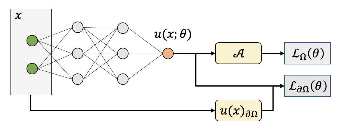
Figure 1: The training framework of PINN

PINN is a deep neural work $u(x;\theta)$ with parameters $\theta$ to approximate $u(x)$. The optimal parameters $\theta^{*}$ are located by solving the following optimization problem:

$$\theta^{*} =\arg\min_{\theta\in\Theta}\mathcal{L}(\theta)$$

$$=\arg\min_{\theta\in\Theta}\mathcal{L}_{\Omega}(\theta)+\lambda\mathcal{L}_{\partial\Omega}(\theta)$$ (3)

where $\Theta$ is the parameter space, $\lambda$ is a trade-off factor balancing the PDE loss $\mathcal{L}_{\Omega}(\theta)$ and the boundary loss $\mathcal{L}_{\partial\Omega}(\theta)$, and $\mathcal{L}$ is the overall loss of PINN. As shown in Figure 1, the PDE loss $\mathcal{L}_{\Omega}(\theta)$ usually follows a self-supervised training manner with $L^{2}$ loss, i.e.,

$$\mathcal{L}_{\Omega}(\theta)=\|\mathcal{A}(x;u(x;\theta))\|_{2,\Omega}^{2}$$

The operator $\mathcal{A}$ can be implemented through the automatic differentiation engine of deep neural networks. The boundary loss $\mathcal{L}_{\partial\Omega}(\theta)$ is commonly derived through supervised training with $L^{2}$ loss, i.e.,

$$\mathcal{L}_{\partial\Omega}(\theta)=\|\mathcal{B}(x;u(x;\theta))\|_{2,\partial\Omega}^{2}=\|u(x;\theta)-u(x)\|_{2,\partial\Omega}^{2}$$

Here, $u(x)$ is the ground truth solution of the problem on the boundary. Note that, for $x$ on the boundary, it can be included in both $\mathcal{L}_{\Omega}(\theta)$ and $\mathcal{L}_{\partial\Omega}(\theta)$. Denote $r(x;\theta)=|\mathcal{A}(x;u(x;\theta))|$ as the approximation residual of the PINN. The above $L^{2}$-norm is defined as

$$\|r\|^{2}_{2,\Omega}=\int_{\Omega}r(x;\theta)^{2}\omega(x)d(x)$$

where $\omega(x)$ is the prior distribution of the problem.

In the actual neural network training scheme, the optimization problem (2.2) is reconstructed following a supervised learning framework. Instead of the directly calculated on entire $\Omega$, the loss function is approximated on a training dataset which is collected following the prior distribution on $\Omega$. The training dataset consists of collocation points $\mathcal{D}=\{s^{(n)}\}_{n=1}^{N}$ and boundary points $\mathcal{D}_{b}=\{s_{b}^{(n)}\}_{n=1}^{N_{b}}$. The loss function is the empirical risk on the training dataset, i.e.,

$$\hat{\mathcal{L}}(\theta)=\hat{\mathcal{L}}_{\Omega}(\theta)+\lambda\hat{\mathcal{L}}_{\partial\Omega}(\theta)$$

where

$$\hat{\mathcal{L}}_{\Omega}(\theta)=\frac{1}{N}\sum_{n=1}^{N}\|r(s^{(n)};\theta)\|_{2}^{2},\;\;\;\;\;\hat{\mathcal{L}}_{\partial\Omega}(\theta)=\frac{1}{N_{b}}\sum_{n=1}^{N_{b}}\|u(s_{b}^{(n)};\theta)-u(s_{b}^{(n)})\|_{2}^{2}$$

Note that, as discussed above, $\mathcal{D}_{b}$ can be a subset of $\mathcal{D}$. Although $\mathcal{D}$ and $\mathcal{D}_{b}$ are unbiased samples collected from $\omega(x)$, there is still a gap between the generalization risk $\mathcal{L}(\theta)$ and the empirical risk $\hat{\mathcal{L}}(\theta)$. The gap is

$$\mathcal{G}(\theta) =|\mathcal{L}(\theta)-\hat{\mathcal{L}}(\theta)|$$

$$=|\mathcal{L}_{\Omega}(\theta)+\lambda\mathcal{L}_{\partial\Omega}(\theta)-(\hat{\mathcal{L}}_{\Omega}(\theta)+\lambda\hat{\mathcal{L}}_{\partial\Omega}(\theta))|$$

$$\leq|\mathcal{L}_{\Omega}(\theta)-\hat{\mathcal{L}}_{\Omega}(\theta)|+\lambda|\mathcal{L}_{\partial\Omega}(\theta)-\hat{\mathcal{L}}_{\partial\Omega}(\theta)|$$

Consider the gap between the generalization risk and the empirical risk of the PDE loss for now. Since $\{s^{(n)}\}_{n=1}^{N}$ are i.i.d. samples drawn from $\omega(x)$, and assume $a\leq r(s^{(n)};\theta)\leq b$, $n=1,\ldots,N$, for a small positive non-zero value $\epsilon$, by Heoffding’s inequality

$$\mathbb{P}\left[\left|\mathcal{L}_{\Omega}(\theta)-\hat{\mathcal{L}}_{\Omega}(\theta)\right|>\epsilon\right]\leq 2\exp\left(\frac{-2N\epsilon^{2}}{(b-a)^{2}}\right)$$

If the training sample has larger residual range $b-a$, the upper bound will be tighter. Thus, locating high-residual samples and adding them to the training dataset can be beneficial to shrink the gap.

2.3 Collocation Points Sampling Strategies and Iterative Training

As mentioned in section 1.1, the adversarial training can be related to collocation points sampling strategies. In this section, we will discuss different characteristics of different sampling strategies.

Samples can be drawn independently from the model approximation status, for example the uniform sampling whose samples are independently identical distributed (i.i.d.) with $s^{(n)}\sim\mathcal{U}[\Omega]$. Suppose we have a model already trained on a dataset but fails only in a tiny region. If we try to refine the model with sample drawn by uniform sampling, there will be a low probability that samples fall into the failure region. However, new samples in the failure region can help further improve the model while samples in well-approximated regions have much less significancy as the model are already well trained there. Thus, accurately locating failure regions, especially locating crucial collocation points, can improve the approximation accuracy and the training efficiency. In the PINNs framework, the failure region is located through the residual.

Generating more samples in high-residual regions can be achieved through two main approaches, i.e. residual distribution approximation and sample refinement.

Residual distribution approximation: Although the model residual is accessible on the entire problem domain, as the neural network is non-convex, high-residual regions are difficult to locate. One effective way is approximating the residual map with an artificial distribution then drawing samples from the approximated distribution, which ensures that samples have larger probability generated in high-residual regions. For example, Gao et. al. [28] propose to use gaussian or gaussian mixture to approximate the residual map, which is namely Self-adaptive importance sampling (SAIS). SAIS begins with an random initialization and iteratively adding new samples which follow Gaussian distributions $\mathcal{N}(\mu,\Sigma)$. The Gaussian distributions are estimated from the sampling distribution of the residual and truncated to be restricted to the problem domain.

$$\mu =\frac{1}{N_{p}}\sum_{n=1}^{N_{p}}\tilde{s}^{(n)}$$

$$\Sigma =\frac{1}{N_{p}-1}\sum_{n=1}^{N_{p}}(\tilde{s}^{(n)}-\mu)\otimes(\tilde{s}^{(n)}-\mu)$$

where $\tilde{s}^{(n)}$ are samples with top residuals generated from the Gaussian distribution estimated in the previous iteration. Correct residual distribution approximation can increase the probability of the samples falling into high-residual regions. But choosing a proper distribution in prior is difficult. SAIS assumes that the distribution is a Gaussian distribution or a mixture of Gaussians and is suitable for use on regions that are shaped like ellipses or collections of ellipses.

Sample refinement: An alternative approach to position samples in high-residual regions is directly moving samples towards high-residual. One of the representative methods is RAR [18]. RAR selects samples with the top-$N$ residuals from a larger sample set generated by uniform sampling, i.e.,

$$\{s^{(n)}\}_{n=1}^{N}=\{\arg\max_{x}r(x;\theta)\}_{N},\forall x\in\{\tilde{s}^{(m)}\}_{m=1}^{\lfloor KN\rfloor}$$

where $K>1$ and $\tilde{s}^{(m)}\sim\mathcal{U}[\Omega]$. Sample refinement should find high-residual regions or directions towards high-residual regions accurately and efficiently. However this search is often effected by the volume of the region and the dimensions of the problem domain. RAR selects high-residual samples from i.i.d. samples such that there will be less samples fall into the high-residual region if the volume of region decrease. By the large deviations theory, the number of candidate i.i.d. sample has to be exponentially increase to maintain the same probability.

The above sampling strategies can be iteratively applied during the training process. Particularly, samples are iteratively generated based on the current approximation status of the model and appended into the training dataset for additional rounds of training [28, 18]. In this case, the collocation points are partitioned as $\mathcal{D}=\cup_{k=1}^{K}\mathcal{D}_{k}$, where $\mathcal{D}_{k}=\{s_{k}^{(n)}\}_{n=1}^{N_{k}}$ are samples generated in the $k$-th training iteration. The model parameters obtained in the previous iteration are loaded and further retrained on $\cup_{i=1}^{k}\mathcal{D}_{i}$ in the $k$-th training iteration. The empirical risk of the collocation points is

$$\hat{\mathcal{L}}(\theta)=\frac{\sum_{i=1}^{k}\sum_{n=1}^{N_{i}}\|r(s_{i}^{(n)};\theta)\|_{2}^{2}}{\sum_{i=1}^{k}N_{i}}$$

3 Adversarial Training for PINNs

3.1 Motivation

Adversarial attacks can move samples towards failure regions by solving the optimization problem (2.1). For PINNs, the equation approximation is preceded through maximizing the residual $r(x;\theta)$. Thus, an adversarial attack can be constructed by moving samples towards higher residuals, particularly towards the local maximums of the residuals with sufficient steps. Since adversarial samples move towards higher residuals, they can automatically and accurately adapt to the failure regions. The failure location adaptation is independent from the volume of the failure region, the dimension of the problem or the distribution of the residual map, which is especially helpful in solving PDEs with specific characteristics such as sharp, oscillatory or multi-peak solutions, etc.

After adversarial samples are generated, we apply adversarial training to force the model to focus on the failure regions, i.e. refine the model with the adversarial samples. Further, under the iterative training framework, adversarial attacks can be applied in each training iteration to generate samples surrounding the residual local maximums. Then, the residual peaks will be suppressed during the adversarial training and new peaks will be captured in the next training iteration. The adversarial attack helps to take samples carefully around, if not exactly at, the local maximums, thus the residual should be better suppressed than taking samples at random positions. Moreover, the procedure is adaptive to all kinds of residual maps which can provide better suitability for various complicated equations.

In the following sections, we will describe the adversarial attack algorithm, named PINN-PGD, in detail. The PINN-PGD is particularly designed to generate adversarial samples for PINNs based on an $L^{\infty}$ constrained PGD attack method. Then, we illustrate the iterative adversarial training framework, named AT-PINN. The AT-PINN extends the basic adversarial training with sample reinforcement augmentation and revisiting as hyper-parameters to control the sampling during the training iteration. The effects of all the hyper-parameters will be discussed and verified in section 4.5.

3.2 PINN-PGD

For the regression problem of (2.1), we extends the basic PGD attack as in Algorithm 1. In the random initialization step, an uniformly distributed random variable $\mathcal{U}[-\epsilon,\epsilon]$ is added to the original sample $x$. Then the perturbed sample is clipped back to the problem domain $\Omega$. In the projected gradient descent process, as we are maximizing the residual, gradient ascent are applied. The model takes a step of $\eta$ to the direction of the loss gradient each time. The overall perturbation is clipped within the maximum perturbation threshold $[-\epsilon,\epsilon]$. Finally, the perturbed sample is clipped to ensure that the adversarial sample still belongs $\Omega$.

Algorithm 1 PINN-PGD

0:  The original sample $x$, the problem domain $\Omega$, the regression model $r(x;\theta)$, the target function $r(x)$, the loss $\mathcal{L}(\cdot)$, the maximum perturbation threshold $\epsilon$, number of iteration steps $T$, and the step size of each iteration $\eta$.

1:  $g_{0}\leftarrow 0$

2:  $x\leftarrow x+\mathcal{U}[-\epsilon,\epsilon]$ $\triangleright$ Random initialization

3:  $x\leftarrow clip_{\Omega}(x)$

4:  for $t=1:T$ do

5:     $g_{x}\leftarrow\eta*sign\big{(}\nabla_{x}r(x;\theta)\big{)}$$\triangleright$ Gradient ascent

6:     $g_{0}\leftarrow clip_{[-\epsilon,\epsilon]}(g_{0}+g_{x})$

7:  end for

8:  $x\leftarrow x+g_{0}$

9:  $x\leftarrow clip_{\Omega}(x)$

3.3 AT-PINN

AT-PINN follows the iterative training framework. At initialization, $N_{0}$ samples $\{s_{0}^{(n)}\}_{n=1}^{N_{0}}$ are generated through the LHS. Then, at the iteration $k$, we calculate the adversarial samples $\{a^{(n)}_{k}\}_{n=1}^{N_{k-1}}$,$\ldots$, $\{a^{(n)}_{k-m}\}_{n=1}^{N_{k-m-1}},\{a_{1}^{(n)}\}_{n=1}^{N_{0}}$ for all the samples generated in the previous $m$ iterations and the initial samples, i.e., $\{s^{(n)}_{k-1}\}_{n=1}^{N_{k-1}}$, $\ldots$, $\{s^{(n)}_{k-m-1}\}_{n=1}^{N_{k-m-1}},\{s_{0}^{(n)}\}_{n=1}^{N_{0}}$. The calculated adversarial samples are used as candidate samples. New samples are selected from the $N_{k}$ highest residual candidate samples, where $N_{k}$ is the number of samples of the $k$-th iteration. The purpose of revisiting the samples in the previous $m$ iterations is to speed up the convergence of the samples to the high residual areas. And revisiting the initialization samples is to avoid the iteration getting stuck in local regions. The model is then retrained on new samples before the next adversarial training iteration starts. The details can be found in Algorithm 2.

Algorithm 2 AT-PINN

0:  The model $u(x;\theta)$, the residual $r(x;\theta)$ of model, the number of training iterations $K$, the number of sampling points in each iteration $N_{k}$, $k=0,\ldots,K$, the problem domain $\Omega$, the maximum perturbation threshold $\epsilon$, the number of iteration steps $T$, the step size of each iteration $\eta$, and the number of revisiting iterations $m$.

1:  Sample $\{s_{0}^{(n)}\}_{n=1}^{N_{0}}$ through LHS

2:  $u(x;\theta)\leftarrow$ train on $\{s_{0}^{(n)}\}_{n=1}^{N_{0}}$

3:  for $k=1:K$ do

4:     for $i=(k-1-m):(k-1)$ do

5:        $\{a_{i+1}^{(n)}\}_{n=1}^{N_{i}}\leftarrow\{\text{PINN-PGD}(s_{i}^{(n)},|r(x;\theta)|,\epsilon,\eta,T,\Omega)\}_{n=1}^{N_{i}}$

6:     end for

7:     $\{a_{1}^{(n)}\}_{n=1}^{N_{i}}\leftarrow\{\text{PINN-PGD}(s_{0}^{(n)},|r(x;\theta)|,\epsilon,\eta,T,\Omega)\}_{n=1}^{N_{0}}$

8:     $\{s_{k}^{(n)}\}_{n=1}^{N_{k}}\leftarrow$ $\{\arg\max_{x}r(x;\theta)\}_{N_{k}}$, $\forall x\in\left(\cup_{i=k-m}^{k}\{a_{i}^{(n)}\}\right)\cup\{a_{1}^{(n)}\}$

9:     $u(x;\theta)\leftarrow$ retrain on $\left(\cup_{i=0}^{k}\{s_{i}^{(n)}\}\right)$

10:  end for

From the optimization point of the view, AT-PINN is similar as local maximum searching for non-convex function using a gradient-based method from multiple initial points. The difference is that AT-PINN has constrains on the number of iteration steps and the searching distance which retain the sample surrounding the maximums instead of converging at them.

3.4 Sampling Strategies Comparison

As illustrated in Figure 2, if the model has a sharp solution, it usually has one dominant peak in the residual. Since the area of the residual peak can be very small, the probability of samples fall onto the peak will be low if uniform sampling strategy is taken. If an adaptive Gaussian sampling is applied, the samples will gather around the peak and leave the remaining areas of the problem domain less sampled. If we use uniform sampling as initialization points (first column of Figure 2) and apply adversarial attack to generate samples, the samples near the peak will move to the peak while samples in the remaining areas will not move much. For the problem with oscillatory solution, the uniform sampling can fail to describe every peaks and the adaptive Gaussian sampling can miss the peaks far away from the mean of the distribution. However, adversarial attack sampling can capture every peaks as long as samples are initialized near every peaks. As we demonstrated in Figure 2 (b), we took uniform sampling as initialization, adversarial attack can locate all the peaks in the residual map. The situation is similar in the multi-peak solution problem as shown in Figure 2 (c), the adversarial samples can sufficiently describe the distribution of the residual even though its distribution is complicated to be expressed explicitly.

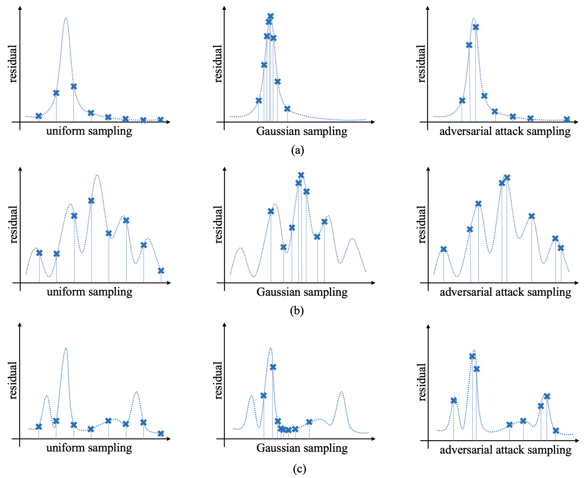
Figure 2: The residual and samples of (a) a sharp solution, (b) an oscillatory solution, (c) a multi-peak solution problem.

4 Numerical Experiments

4.1 Two-dimensional Poisson equation

In the first numerical experiments, we consider the following two-dimensional Poisson equation:

$$-\Delta u(x,y)=f(x,y)\;\;\;\;\; \text{in }\Omega$$

$$u(x,y)=g(x,y)\;\;\;\;\; \text{on }\partial\Omega$$ (4)

where $\Omega=[-1,1]^{2}$ and the solution is

$$u(x,y) =exp\big{(}{-100(x-.8)^{2}}\big{)}+exp\big{(}{-100x^{2}}\big{)}+exp\big{(}{-100(x+.8)^{2}}\big{)}$$

$$-exp\big{(}{-100(y-.8)^{2}}\big{)}-exp\big{(}{-100y^{2}}\big{)}-exp\big{(}{-100(y+.8)^{2}}\big{)}$$ (5)

The true solution is shown in Figure 3 which contains three ridges at $x=\{-0.8,0,0.8\}$ and three canyons at $y=\{-0.8,0,0.8\}$.

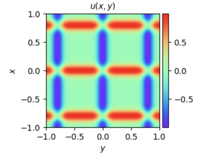
Figure 3: True solution of the two-dimensional Poisson equation

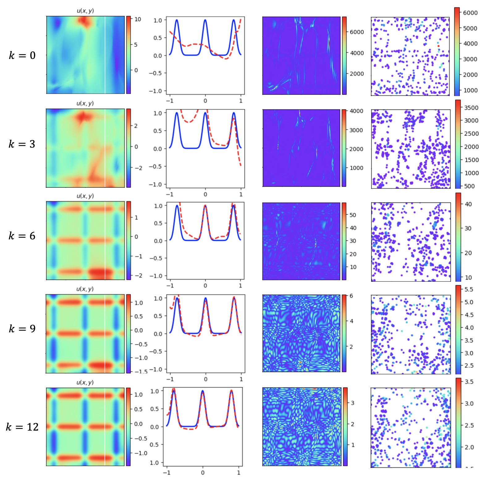
Figure 4: AT-PINN for the two-dimensional Poisson equation. (1st column) model prediction at the test dataset; (2nd column) blue solid: equation solution at $x=0.5$, red dashed: model prediction; (3rd column) model prediction residual on the test dataset; (4th column) samples generated by AT-PINN.

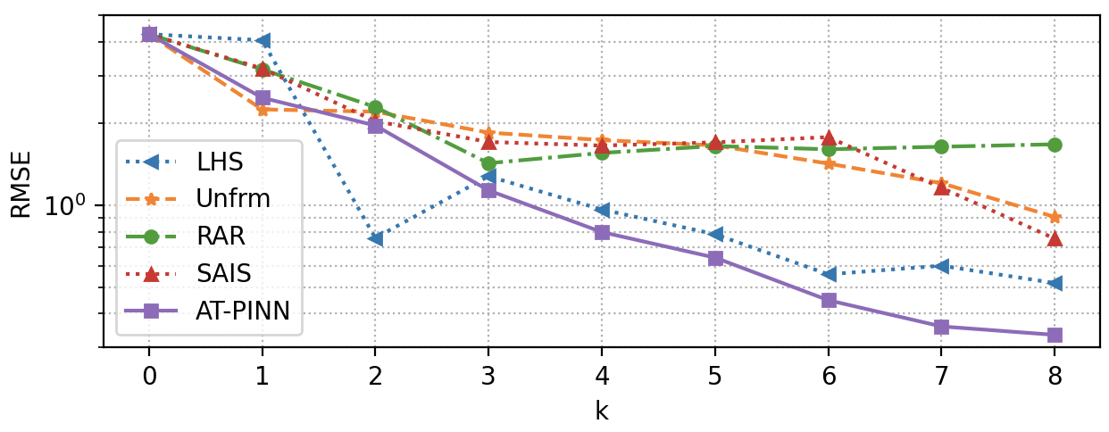
Figure 5: The RMSE of solution on the test dataset for the Poisson equation.

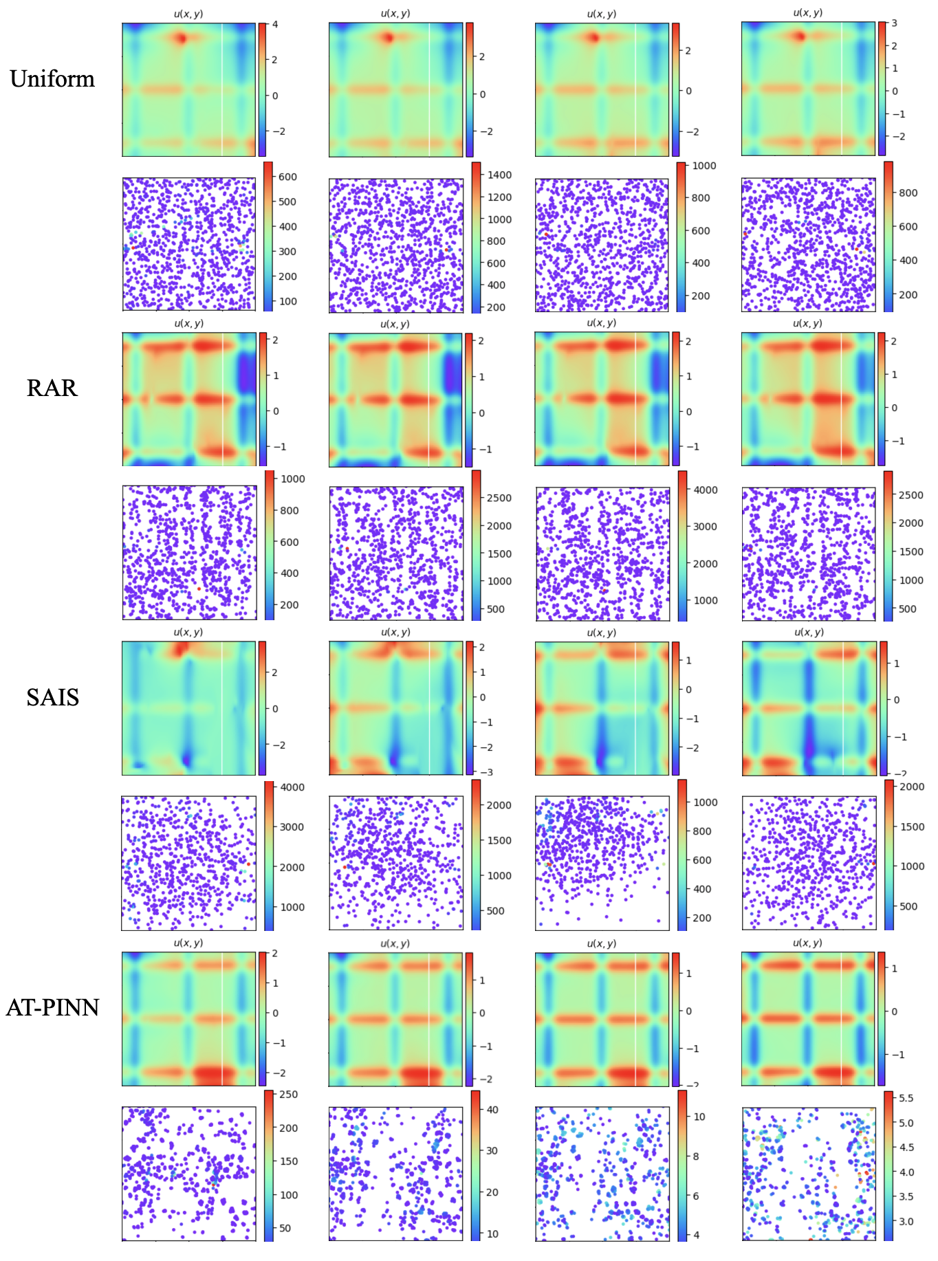
Figure 6: Samples generated by uniform sampling, RAR, SAIS, and AT-PINN at $k=5$ (1st column), $k=6$ (2nd column), $k=7$ (3rd column) and $k=8$ (4th column) for the Poisson equation.

Experiment setup: The PINN model is a fully connected neural network with 8 hidden layers and 20 neurons in each layer. The number of boundary points ($N_{b}$) is set to $200$. The model is first trained on $500$ Latin hypercube sampling points ($N_{0}=500$) for $200,000$ epochs ($ep_{0}=2\text{e}5$) using Adam optimizer with learning rate $lr=0.0001$. In the subsequent iterations, $N_{1}=500$, $ep_{1}=5\text{e}4$ and $N_{i}=1,000$, $ep_{i}=5\text{e}4$ for $i\geq 2$. The momentum of the Adam optimizer is reset to $0$ before each retrain. The detailed parameter settings for each sampling strategy are as follows:

1. AT-PINN: the number of revisiting iterations $m=1$, the maximum perturbation threshold $\epsilon=0.1$, the number of iteration steps $T=20$, and the step size of each gradient ascent iteration $\eta=0.02$.

2. SAIS: the number of each sampling is set to $300$, the parameter $p_{0}=0.1$, and the maximum updated number $M=10$.

3. RAR: we always sample twice the number of samples and select the top half samples maximizing the residual.

We use LHS as the baseline sampling method. LHS baseline doesn’t follow the iterative training. The model is trained with all the samples in one time for $50,000$ epochs. Models are tested on a grid that discretizes each dimension by 256.

In Figure 4, we demonstrate the AT-PINN for Equation (4.1). When $k=0$ (the first row of Figure 4), the model was trained on $N_{0}$ samples generated by LHS. The model prediction is significantly different from its true solution. The relative mean-squared-error (RMSE) is $4.271$. The residual $r(x;\theta)$ has the highest amplitude more than $6,000$ on the test dataset. Then, AT-PINN is applied to generate adversarial samples based on the $N_{0}$ initialization samples. The largest amplitude of adversarial samples exceeds $6,000$ as well, which indicates that the adversarial attack is good at locating local maxima of the residual. When the training iteration reaches $k=6$, the model prediction is much closer to the true solution. The RMSE decreases to $0.642$. The distribution of the adversarial samples coincides with the residual, i.e. the regions of high residual acquired more adversarial samples. As $k=12$, the RMSE reaches $0.256$. The largest residual is around $3.5$. The adversarial samples distribute similar as the distribution of the residual and the largest residual of adversarial samples is also around $3.5$. The experiment shows that, by applying AT-PINN to Equation (4.1), the model is converging to the true solution as the number of training iteration $k$ increases.

The performance comparisons of AT-PINN with other sampling strategies, including LHS, uniform sampling, RAR, and SAIS, are shown in Figure 5. The training of LHS is not stable. We choose to plot one of the training that converges to the true solution but most of the time LHS doesn’t converge. The model trained with $2,000$ samples can have much lower RMSE than the model trained with $3,000$ samples. When $8,000$ LHS samples are applied to train the model, its RMSE is $0.518$. The model trained with RAR method has the lowest RMSE $1.430$ at $k=3$, while the accuracy doesn’t further increase as the number of training samples increases. The uniform sampling and the SAIS converge to the true solution as $k$ increase. The RMSEs at $k=8$ for uniform sampling and SAIS are $0.906$ and $0.754$, respectively. The model trained with adversarial samples has the best performance which reaches the RMSE $0.333$ at $k=8$.

We further plot the generated samples of all the tested sampling strategies from $k=5$ to $k=8$. As shown in Figure 6, the uniform sampling generates samples independently from the current approximation error. RAR selects samples from the uniform sampling with larger residuals. Thus, the sampling spans the entire problem domain, but regions with higher residual has relative denser samples. SAIS draws samples from an Gaussian distribution approximated according to the residual. However, the distribution of the residual is not Gaussian, which results inaccurate high-residual-region locating. AT-PINN adapts its sampling to the residual. A large portion of the adversarial samples have high residuals, while only a few samples have high residuals in those generated by the other sampling strategies. Furthermore, it is worth noting that when it comes to uniform sampling, RAR, and SAIS, there is a noticeable increase in the highest sample residual between values of $k=5$ and $k=8$. To illustrate, in the SAIS method, the maximum sample residual at $k=7$ is approximately $1,000$, while at $k=8$ it goes up to around $2,000$ (in row 6). In contrast, the highest sample residual consistently decreases throughout the entire training process of AT-PINN. It indicates that the adversarial attack is capable of locating local maximums throughout the residual map and the iterative training can effectively suppress them. As for the correlation between failure regions and sample densities, adversarial samples successfully gather at failure regions, i.e. the canyons and ridges. The SAIS method draws most of the samples in the averaged position of all the high-residual regions.

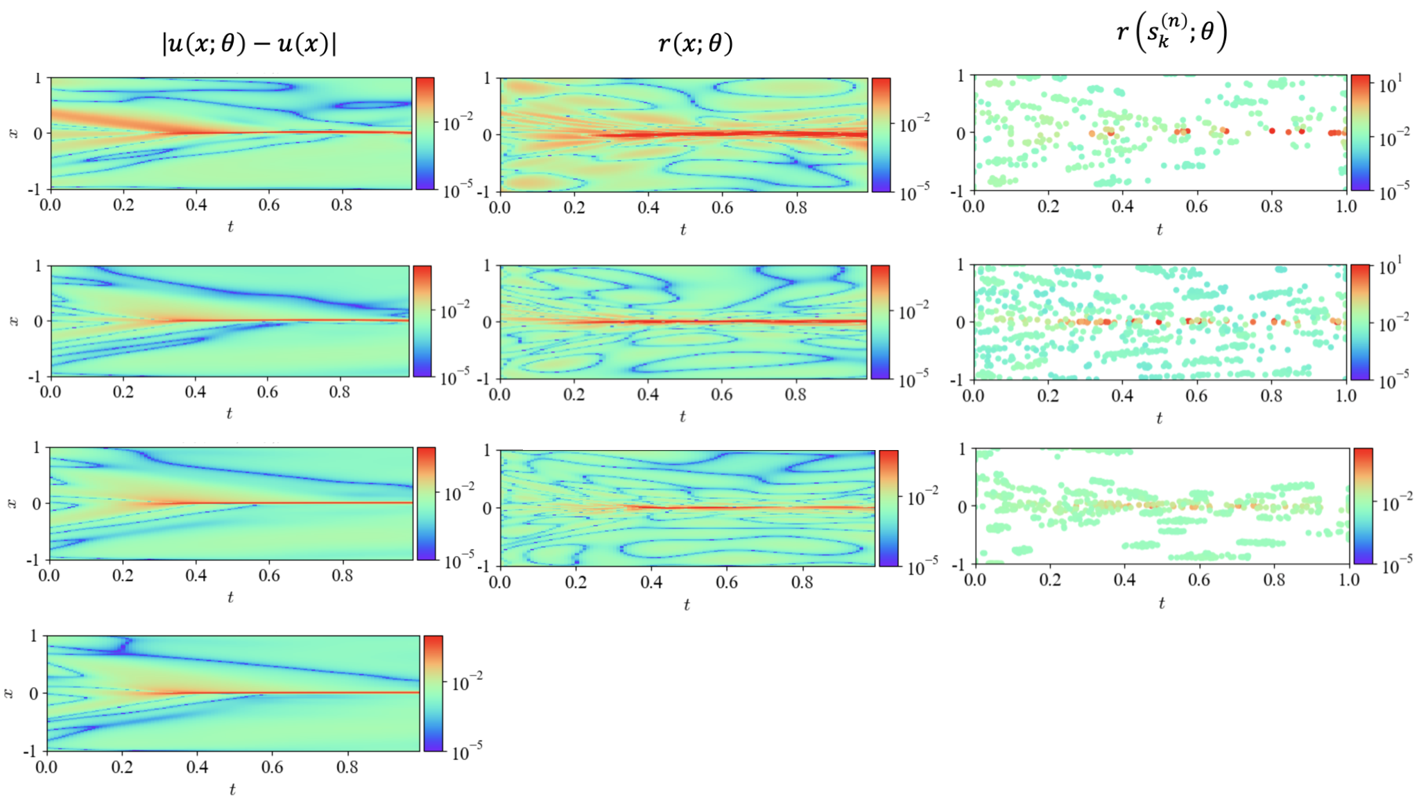
Figure 7: AT-PINN for the Burgers’ equation at $k=0$ (1st row), $k=1$ (2nd row), $k=2$ (3rd row) and $k=3$ (4th row).

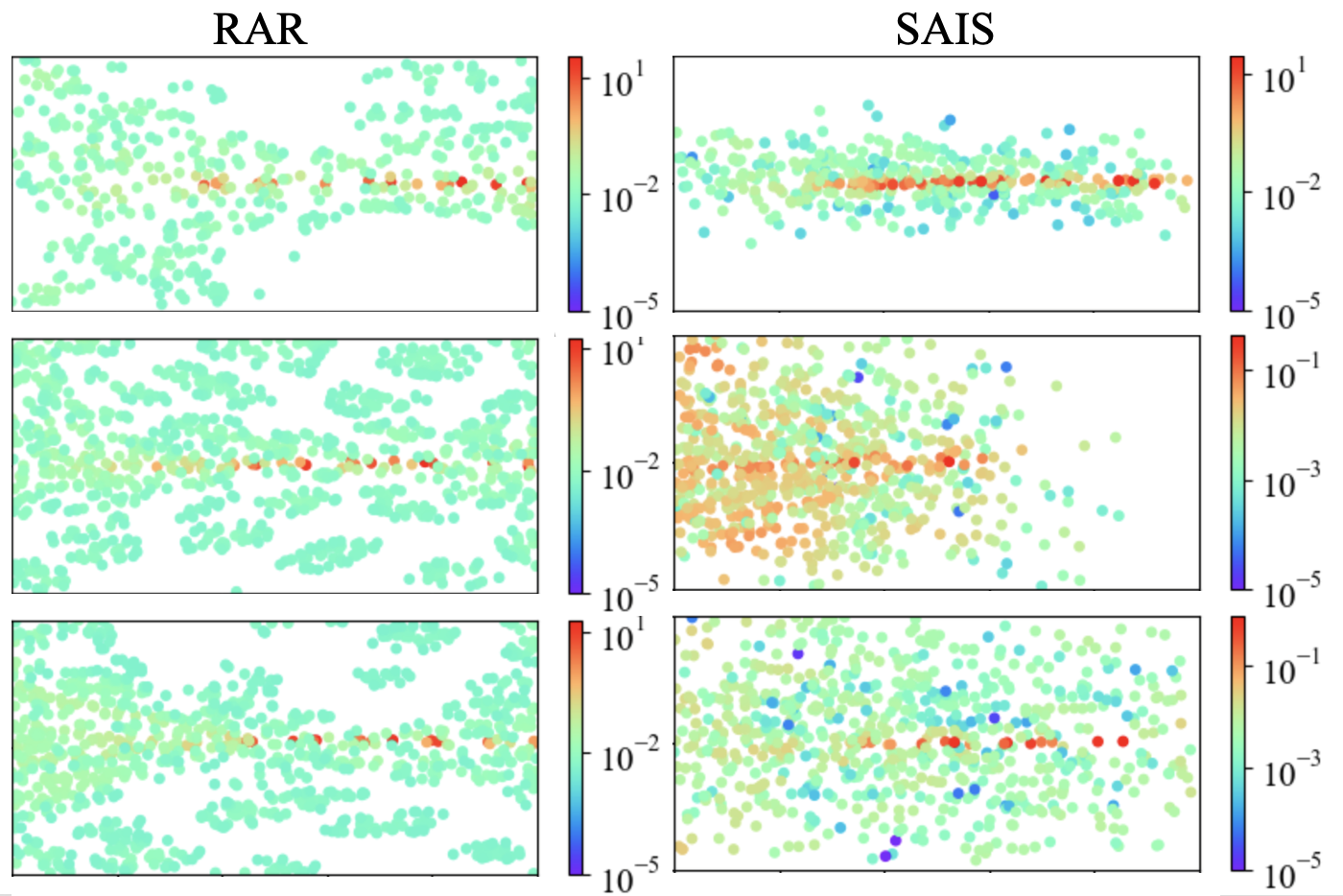
Figure 8: Samples generated by RAR and SAIS at $k=0$ (1st row), $k=1$ (2nd row), and $k=2$ (3rd row) for Burgers’ equation.

4.2 Burgers’ Equation

Consider the following Burgers’ equation:

$$u_{t}+uu_{x}-(0.01/\pi)u_{xx}=0$$

$$u(x,0)=-sin(\pi x)$$

$$u(t,-1)=u(t,1)=0$$

where $(x,t)\in[-1,1]\times[0,1]$.

Experiment setup: All of the model settings and sampling parameters in this experiment are based on the setup of the two-dimensional Poisson equation experiment, with the exception of $N_{b}=100$, $ep_{0}=1\text{e}5$, $ep_{1}=2\text{e}5$ and $ep_{2}=1\text{e}5$. The training epochs are adjusted to ensure sufficient training.

The training process for the Burger’s equation using AT-PINN is demonstrated in Figure 7. Initially, before the adversarial attack training iteration starts ($k=0$), the error and residual in the regions around $x=0$ and $t<0.5$ are relatively larger compared to other regions. AT-PINN adaptively generates more training samples in these regions. Additionally, the sample residuals are close to the highest residual in the entire problem domain, indicating the effectiveness of the adversarial attack. After one round of adversarial training at $k=1$, the prediction error and residual in the region $t<0.5$ are successfully suppressed. The regions with large error and residual around $x=0$ are significantly reduced. As the training progresses to $k=2$ and $k=3$, the error and residual of the model are further decreased, and the generated samples gradually gather towards the remaining region with high residual.

Figure 8 shows a comparison between the samples generated by RAR and SAIS. RAR selects the top-residual samples to refine the sampling towards high-residual regions. While approximating the Burgers’ equation, high-residuals are predominantly located at $x=0$. As the iterative training progresses and the high-residual region diminishes, the probability of uniformly generated samples falling into this region decreases. On the other hand, SAIS employs Gaussian distribution re-estimations during the iterative training process. However, the distribution of the high-residual region is not a typical Gaussian. As for the AT-PINN, the adversarial attack finds the local maximum of the model residual, effectively moving the samples towards the high-residual regions. The adversarial samples generated during the iterative training can be seen as random walks. The random walk ensures that new samples remain related to the samples generated in the previous iteration, which was located in high-residual regions in the previous iteration. Moreover, the revisiting mechanism, is similar to RAR, further reinforces the selection of high-residual samples. From the numerical experiments of the two-dimensional Poisson equation and Burgers’ equation, AT-PINN can adapt to any residual distribution without relying on prior assumptions. Thus, AT-PINN is suitable to be applied on equations with complicated or sharp solutions.

During the PINN training, the lowest RMSE of the solution $0.0545$ are reached by AT-PINN at $k=2$. The SAIS method also achieves a similar RMSE but with $1,000$ additional samples at $k=3$. RAR yields an RMSE of $0.287$ at $k=3$. By using uniform sampling and LHS, the RMSE is reduced to $0.122$ and $0.0963$ at $k=3$, respectively. It is worth mentioning that the lowest RMSE obtained for the same structure on Burgers’ equation is around $0.05$, which has been verified in [40]. Thus, the rest iterations are neglected in Figure 9. Comparing AT-PINN and SAIS, the adversarial attack locates both the high-residual regions at $t<0.5$ and $t=0$ since $k=1$. It results a better approximation at the $t=0.25s$ cross section. However, SAIS only locates the high-residual region at $t=0$ when $k=1$. Thus, the approximation is slightly biased at the $t=0.25s$ cross section at $k=1$ and $k=2$.

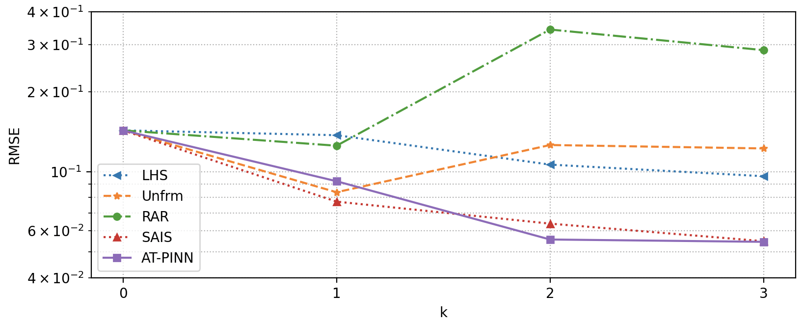
Figure 9: The RMSE of solution on the test dataset for Burgers’ equation.

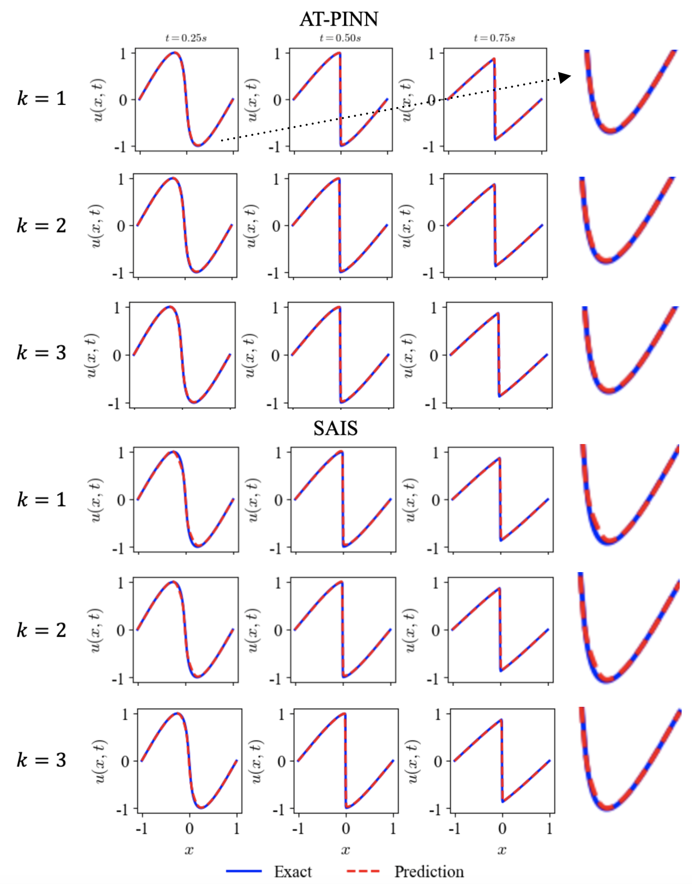
Figure 10: The Burgers’ equation approximation at $t=0.25s$, $t=0.5s$ and $t=0.75s$ cross sections.

4.3 A Multiscale Problem

It has been found that the vanilla PINN fails to solve multi-scale problems [41]. For example, consider the following elliptic equation:

$$-\nabla\cdot(\kappa\nabla u(x))=f \;\;\;\;\;\text{in }\Omega$$

$$u(x)=0 \;\;\;\;\;\text{on }\partial\Omega$$ (6)

where $\Omega=[0,\pi]$ and $f=sin(x)$. If $\kappa(x)$ has multi-scale properties, for example $\kappa(x)=0.5sin(2\pi x/\varepsilon)+sin(x)+2$, where $\varepsilon=1/4$, PINN cannot converge to a satisfied solution. In this experiment, we demonstrates that by employing proper sampling strategies, the model can effectively approximate the multi-scale problem.

Experiment setup: The PINN model structure, optimizer, and learning rate settings follow the setup of the two-dimensional Poisson equation experiment. The sampling and training parameters are as follows: $N_{i}=200$, $ep_{i}=3\text{4}$ for $i\geq 0$. For the AT-PINN method, $m=2$, $\epsilon=0.2$, and $T=2$. The remaining parameter settings for AT-PINN and other sampling strategies are kept unchanged. A scale of $200$ is multiplied to the boundary loss for all sampling strategies to balance the effect of having fewer boundary sampling points compared to collocation sampling points in one-dimensional problems. The adversarial attack parameters are adjusted in order to allow the model to explore the problem domain adequately before focusing on local maxima.

In Figure 12, we demonstrates AT-PINN for the problem (4.3). As $k=0$, the model fails to learn the problem solution. The model prediction is a smooth curve with small amplitude and the residual shows high-frequency oscillations. AT-PINN generates more samples where the residuals are larger. From $k=1$ to $k=6$, the model gradually converges to the true solution. Although the residual still contains high-frequency components, its oscillations amplitude is compressed within a much smaller range. When we keep increasing $k$, the model can successfully approximate the equation.

Comparing to AT-PINN, uniform sampling and SAIS can also approximate the equation (4.3) to some extent. As shown in Figure 13, when $k=0$, the variance of the residual is small and samples are concentrated in a small region. As $k$ keeps increasing, the approximation accuracy goes higher. However, most samples are generated in the central region instead of around the initial values. This is because of the mis-match between the residual distribution and the artificial assumed distribution. It results slower convergence and larger error comparing to AT-PINN, which is more obvious in Figure 11.

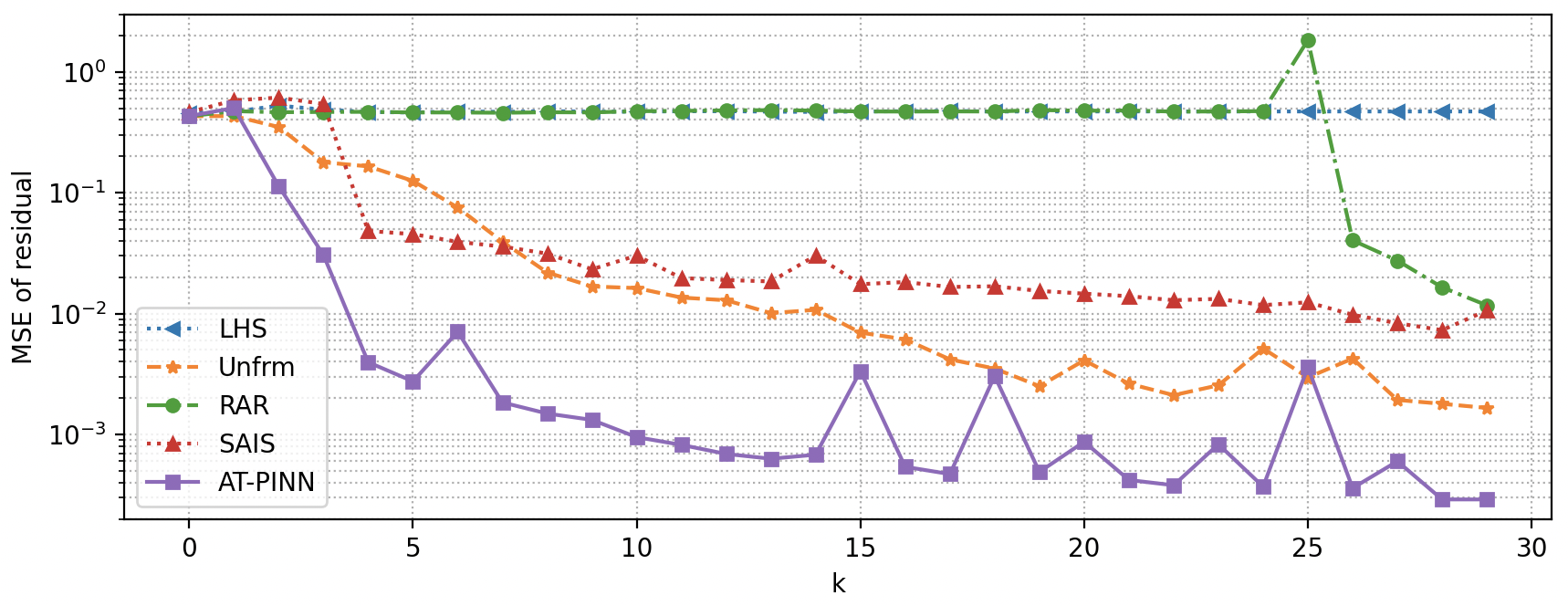
Figure 11: The MSE of the residual on the test dataset for the multi-scale problem.

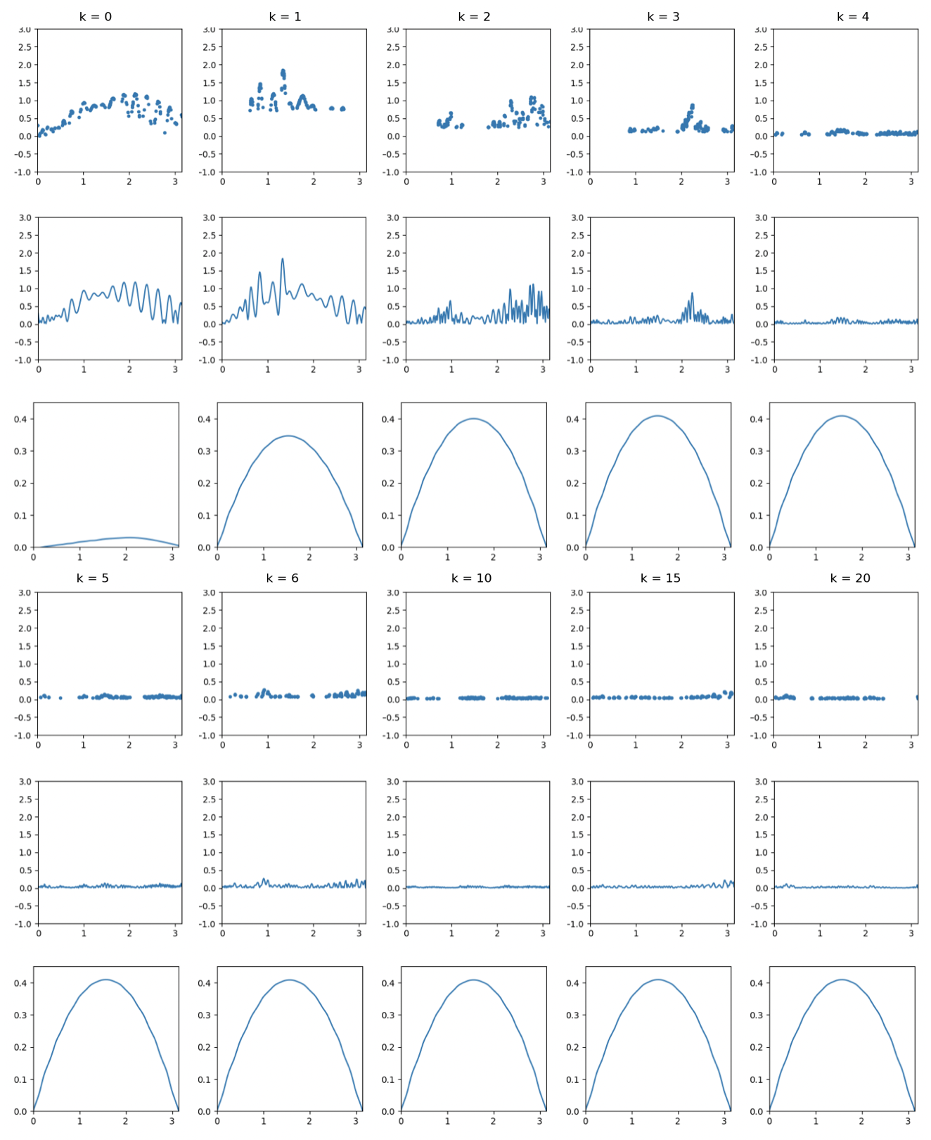
Figure 12: AT-PINN for the multi-scale elliptic equation. (1st row) adversarial samples; (2nd row) model residual; (3rd row) model prediction.

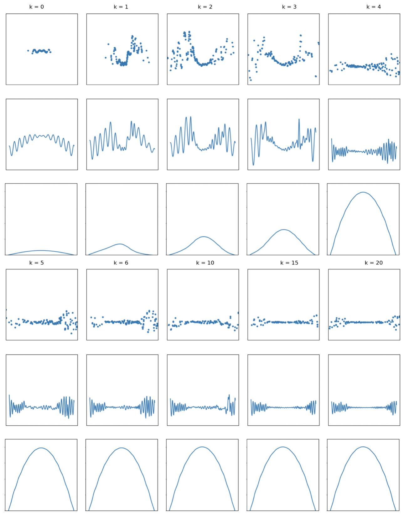
Figure 13: SAIS for the multi-scale elliptic equation. (1st row) SAIS samples; (2nd row) model residual; (3rd row) model prediction.

4.4 Allen-Cahn Equation

There are also reports that PINN may violate physical causation [42], for example the Allen-Cahn equation in the following form:

$$u_{t}=Du_{xx}+5(u-u^{3})$$

$$u(x,0)=x^{2}\cos(\pi x)$$

$$u(-1,t)=u(1,t)=0$$ (7)

where $(x,t)\in[-1,1]\times[0,1]$ and $D=0.0001$. While solving the Alen-Cahn equation with PINNs, the residual is large near the initial state and decays to nearly zero after t = 0.5. We yield that the PINN fails because it accidentally converged to a local minimum and the optimizer are not capable of dragging the model out. The PINN approximation has a large flatten area around $u=0$, as $u=0$, $u_{xx}=0$, $u_{t}=0$ is actually a zero point for the residual $u_{t}-Du_{xx}-5(u-u^{3})$.

Wang et. al. [42] propose to solve the Allen-Cahn equation with causal-PINN. The causal-PINN manages temporal weights such that samples near the initial state are set to higher weights, and samples at later times are gradually set to higher weights. However, the weights have to be manually adjusted according to the number of sampling points and the training requires a large amount of collocation points. In the following numerical experiments, we shows that AT-PINN can adaptively conduct the causal inference along the temporal direction if we set initialization samples near the initial state.

As shown in Figure 14, we first train the PINN on $500$ collocation points within $0\leq t\leq 0.2$ sampled by LHS. From the absolute error of the solution and the residual (as shown in the first two plots in the 1st row), the model can accurately approximation the equation when $0\leq t\leq 0.2$. The adversarial attack try to find the failure regions near the $500$ collocation points and the boundary points, thus the adversarial samples move along the temporal direction adaptively (as shown in the 3rd plot in the 1st row). As the iterative training processes, some adversarial samples adaptively keep moving towards the temporal direction while the rest adversarial samples reinforce the earlier temporal region as shown at $k=1$ and $k=2$. At $k=4$, adversarial samples can cover the entire temporal interval. The solution error and the residual are significantly reduced. Start from $k=5$, adversarial samples start to focus on the two ridges and the canyon between the ridges which are the failure regions of the PINN. It can be observed from solution error, the failure regions gradually shrink as more adversarial samples are generated in the failure regions. Figure 14 shows that, AT-PINN can adaptively perform temporal causal inference since the adversarial attack always try to find the failure regions initialing from the samples generated in the previous iteration. In the following, we will describe the experimental setup in detail and demonstrate that the adversarial training can help PINNs approximate the Allen-Cahn equation with higher accuracy and less samples comparing to other sampling strategies.

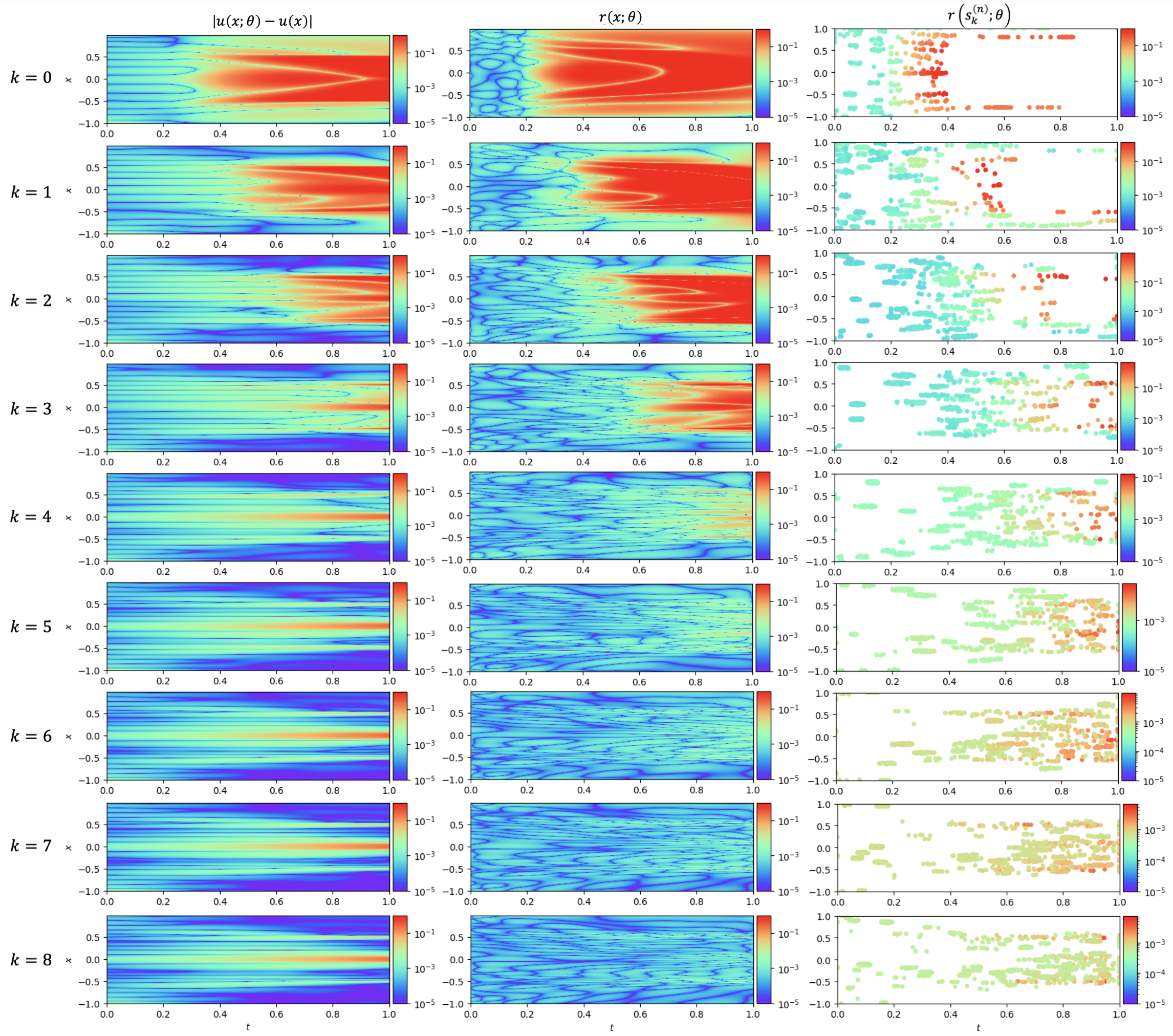
Figure 14: The adaptive temporal causal inference of AT-PINN for the Allen-Cahn equation.

Experiment setup: All of the model settings and sampling parameters in this experiment are based on the setup of the two-dimensional Poisson equation experiment, with the exception of $N_{b}=400$, $N_{i}=500$, $ep_{i}=1\text{e}6$ for $i\geq 0$. The training epochs are adjusted to ensure sufficient training. Additionally, we set $m=1.5$ to slow down the speed of the temporal inference. Specially, we only sample collocation points within $0\leq t\leq 0.2$ at $k=0$ as described above. The maximum perturbation threshold is set to $\epsilon=0.2$ such that with four training iterations in maximum, adversarial samples are capable of covering the entire temporal interval.

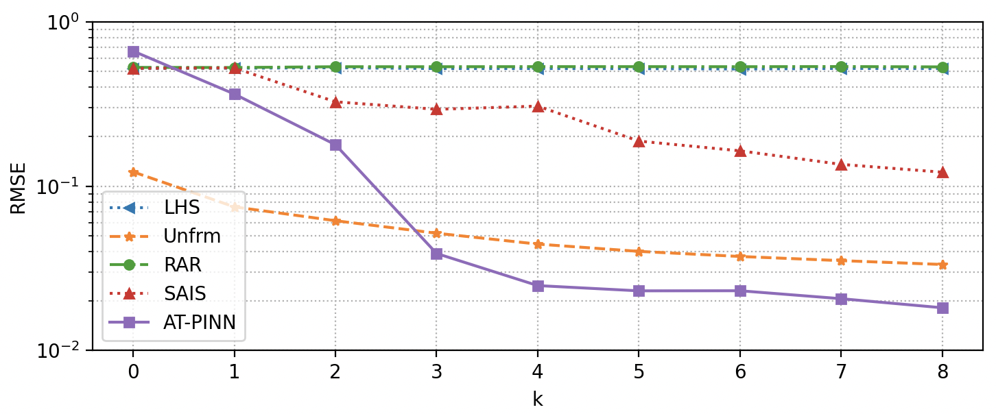
Figure 15: The RMSE of solution on the test dataset. for the Allen-Cahn equation.

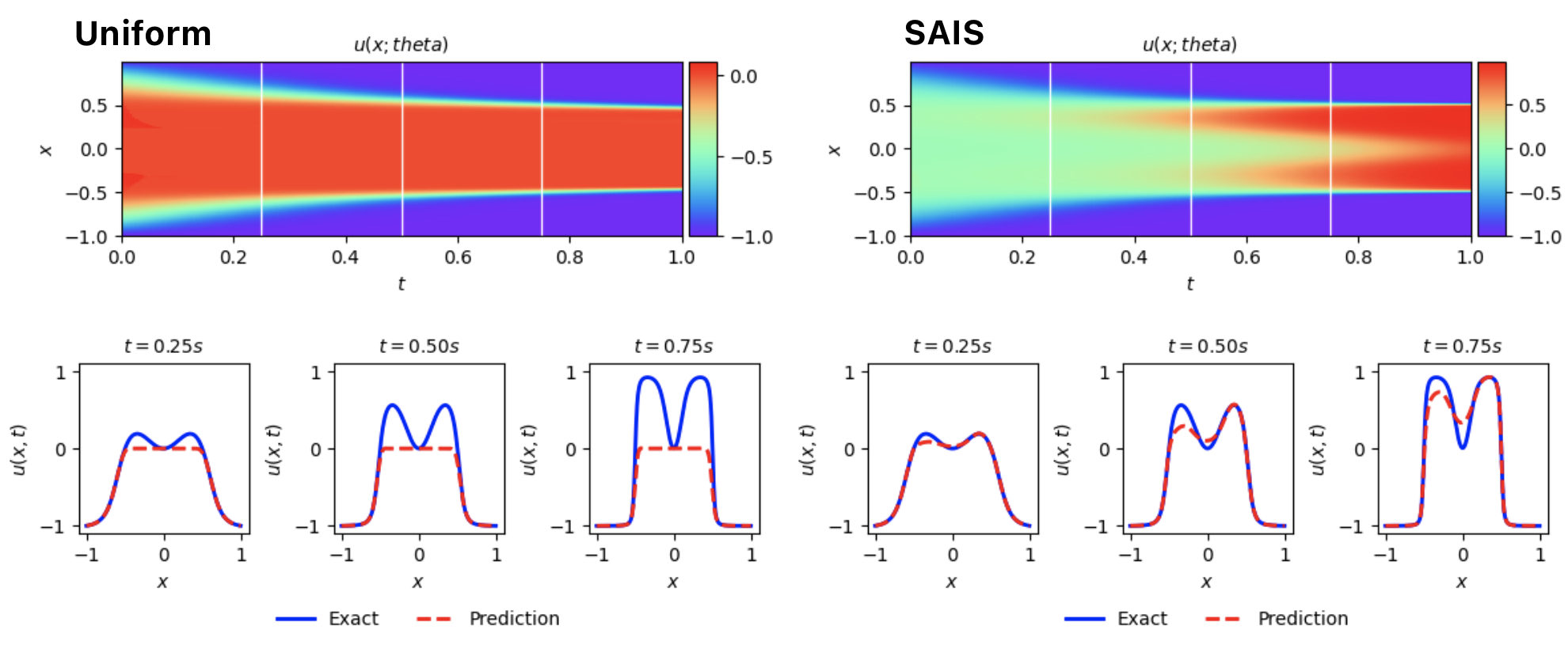
Figure 16: The un-converged uniform sampling and SAIS for the Allen Cahn equation approximation ($k=8$).

In Figure 15, the adaptive behavior of the adversarial training can be observed more clearly. When $k<4$, the RMSE decreases rapidly since the adversarial samples are performing the temporal inference. Later when $k\geq 4$, the adversarial samples pay more attentions to refine the failure regions. The LHS, RAR and uniform sampling can converge to the true solution occasionally. We choose to plot the un-converged cases for LHS and RAR and one of the converged case of the uniform sampling in Figure 15 for better illustration. SAIS helps the PINN slowly converge to the true solution (Figure 16). A detailed comparison between AT-PINN and the occasionally converged PINN through uniform samplings are shown in Figure LABEL:fig:allen_cahn_crosssection. If the achievement rate is not considered, uniform sampling can converge to the true solution even with 500 configuration points. However, uniform sampling can only improve the approximation failure slowly. In contrast, AT-PINN accurately locates the failure regions around $x=0$ and results a much better approximation after $k=4$.

4.5 Hyper-parameter studies for AT-PINN

We demonstrated the performance and adaptive behaviors of the proposed AT-PINN on multi-peak, sharp or oscillatory solutions, as well as temporal causality. The errors of numerical experiments are recored in Table 1. In this section we will study the effect of the AT-PINN hyper-parameters on the multi-scale problem.

PGD is an algorithm that searches for local maxima iteratively, so more iteration steps ($T$) can bring higher accuracy. In adversarial training, more adversarial attack steps can reduce the distance of samples to local maximums of the residual. As shown in Figure 17, when $T$ increases, the adversarial samples are more clustered to the local maximum. In the 1-dimensional multi-scale problem, we chose a much smaller $T$ to get better observations for each failure region rather than the maximum point only. Comparing different number of steps, $T=2$ has the best performance, while all tested adversarial training steps achieve better performance than the uniform sampling.

The revisiting mechanism selects adversarial samples of the most highest residuals. Thus, some small local maximums will be ignored if a larger $m$ is applied. The spread of adversarial samples will shrink, because only large local maximums will be considered. As shown in Figure 18, when $m$ increases, the adversarial samples have larger residual in average. While solving the Allen-Cahn equation, we chose a larger $m$ to reduce the spread speed of adversarial samples towards the temporal direction, such that regions in early time will be sufficiently trained before the regions in later time start to be trained. In the multi-scale problem, we set $m=0$ to make sure no local maximums are ignored, because there are many small residual local maximums in the multi-scale problem. Comparing different revisiting lengths, $m=0$ has the best performance while all tested adversarial training steps achieve better performance than the uniform sampling.

The adversarial attack step size $\eta$ determines the smoothness of the iteration process. Large step size $\eta$ can make the the maximum searching faster but may cause the search trajectory to oscillate. One can adjust $\eta$ according to the volume of the problem domain to adjust the searching speed. In Figure 19, when $\eta=$4e-2, the PGD has better performance locate the local maximums. However, we hope to sample on the entire failure regions instead of at the local maximum points only. Thus, $\eta=$2e-2 is applied to solve the equation and achieved good performance.

The maximum perturbation threshold $\epsilon$ determines the searching range. As shown in Figure 20, if we choose a smaller searching range, i.e. $\epsilon=$1e-1, an AT-PINN with better performance can be obtained. If we chose $\epsilon=$4e-1, the AT-PINN can fail the equation approximation of the multi-scale problem since the adversarial attack may reach a local maximum far away from the initial position.

Table 1: Performance comparison summary of LHS, uniform sampling, RAR, SAIS, and AT-PINN.

RMSE	LHS	Unfrm	RAR	SAIS	AT-PINN
Poisson equation RMSE ($k=8$)	5.2e-1	9.1e-1	1.7e0	7.5e-1	3.3e-1
multi-scale elliptic equation residual MSE ($k=29$)	4.7e-1	1.7e-3	1.2e-2	1.1e-2	2.9e-4
Burgers’ equation RMSE ($k=2$)	1.1e-1	1.2e-1	3.4e-1	6.4e-2	5.6e-2
Allen-Cahn equation RMSE ($k=8$)	5.3e-1	3.3e-2	5.2e-1	1.2e-1	1.8e-2

Figure 17: AT-PINN for the multi-scale problem with different adversarial attack steps ($T$) at $k=0$.

Figure 18: AT-PINN for the multi-scale problem with different adversarial attack revisiting ($m$) at $k=0$.

Figure 19: AT-PINN for the multi-scale problem with different adversarial attack step size ($\eta$) at $k=0$.

Figure 20: AT-PINN for the multi-scale problem with different adversarial attack maximum perturbation threshold ($\epsilon$) at $k=0$.

5 Conclusion and Discussion

In this work, we proposed the AT-PINN training scheme which locates failure regions of PINNs through the PGD-based adversarial attack. The adversarial attack can adaptively generate adversarial samples on failure regions despite their number, the size or the distribution. Such that, AT-PINNs can effectively locate and shrink failure regions while solving complex PDEs, especially those involving multi-scale behaviors or solutions with sharp or oscillatory characteristics. The effectiveness of the proposed AT-PINNs has been verified with numerical experiments including an elliptic equation with multi-scale coefficients, a Poisson equation with multi-peak solutions, and Burgers’ equation with sharp solutions. On the other hand, we found that AT-PINN can inference temporal causality by setting initial samples around the initial value. Its temporal causality behavior has been demonstrated in approximating the Allen–Cahn equation. Numerical experiments show that AT-PINN is self-adapt to various problems benefiting from characteristics of the adversarial attack. Therefore, AT-PINNs can become a general tool for solving complex PDEs.

In the AT-PINN scheme, there are various adversarial attack methods, including non-gradient based white-box attack methods and black-box attack methods, that may be particular effective to particular type of problems. For the adversarial attack, we chose a target attack method which maximize the residual to locate failure regions. Other adversarial attack mechanisms such as non-target attacks can be explored in further works. The iterative training framework can also be further optimized to accelerate the training process, such as adding adversarial samples during training, etc. Beyond the adversarial attack scheme, the failure region locating is actually a non-convex optimization problem which finds all the local maxima. A broader optimization based approaches can be explored for failure region searching. Moreover, adversarial samples during the iterative training are Markov given the residual map, while other sampling strategies assume the samplings are independent. The behavior of different sampling strategies can also be discussed under the stochastic process.

References

- [1] M. Raissi, P. Perdikaris, G. E. Karniadakis, Physics-informed neural networks: A deep learning framework for solving forward and inverse problems involving nonlinear partial differential equations, Journal of Computational physics 378 (2019) 686–707.
- [2] Z. Mao, A. D. Jagtap, G. E. Karniadakis, Physics-informed neural networks for high-speed flows, Computer Methods in Applied Mechanics and Engineering 360 (2020) 112789.
- [3] X. Jin, S. Cai, H. Li, G. E. Karniadakis, Nsfnets (navier-stokes flow nets): Physics-informed neural networks for the incompressible navier-stokes equations, Journal of Computational Physics 426 (2021) 109951.
- [4] R. Mattey, S. Ghosh, A novel sequential method to train physics informed neural networks for allen cahn and cahn hilliard equations, Computer Methods in Applied Mechanics and Engineering 390 (2022) 114474.
- [5] A. Yazdani, L. Lu, M. Raissi, G. E. Karniadakis, Systems biology informed deep learning for inferring parameters and hidden dynamics, PLoS computational biology 16 (11) (2020) e1007575.
- [6] M. Raissi, A. Yazdani, G. E. Karniadakis, Hidden fluid mechanics: Learning velocity and pressure fields from flow visualizations, Science 367 (6481) (2020) 1026–1030.
- [7] G. Pang, L. Lu, G. E. Karniadakis, fpinns: Fractional physics-informed neural networks, SIAM Journal on Scientific Computing 41 (4) (2019) A2603–A2626.
- [8] L. Yuan, Y.-Q. Ni, X.-Y. Deng, S. Hao, A-pinn: Auxiliary physics informed neural networks for forward and inverse problems of nonlinear integro-differential equations, Journal of Computational Physics 462 (2022) 111260.
- [9] D. Zhang, L. Guo, G. E. Karniadakis, Learning in modal space: Solving time-dependent stochastic pdes using physics-informed neural networks, SIAM Journal on Scientific Computing 42 (2) (2020) A639–A665.
- [10] P.-H. Chiu, J. C. Wong, C. Ooi, M. H. Dao, Y.-S. Ong, Can-pinn: A fast physics-informed neural network based on coupled-automatic–numerical differentiation method, Computer Methods in Applied Mechanics and Engineering 395 (2022) 114909.
- [11] Z. Fang, A high-efficient hybrid physics-informed neural networks based on convolutional neural network, IEEE Transactions on Neural Networks and Learning Systems 33 (10) (2021) 5514–5526.
- [12] A. D. Jagtap, K. Kawaguchi, G. E. Karniadakis, Adaptive activation functions accelerate convergence in deep and physics-informed neural networks, Journal of Computational Physics 404 (2020) 109136.
- [13] X. Meng, Z. Li, D. Zhang, G. E. Karniadakis, Ppinn: Parareal physics-informed neural network for time-dependent pdes, Computer Methods in Applied Mechanics and Engineering 370 (2020) 113250.
- [14] S. Wang, S. Sankaran, P. Perdikaris, Respecting causality is all you need for training physics-informed neural networks, arXiv preprint arXiv:2203.07404 (2022).
- [15] J. Yu, L. Lu, X. Meng, G. E. Karniadakis, Gradient-enhanced physics-informed neural networks for forward and inverse pde problems, Computer Methods in Applied Mechanics and Engineering 393 (2022) 114823.
- [16] Z. Z. Kharazmi, Ehsan, G. E. Karniadakis, Variational physics-informed neural networks for solving partial differential equations, arXiv preprint arXiv:1912.00873 (2019).
- [17] E. Kharazmi, Z. Zhang, G. E. Karniadakis, hp-vpinns: Variational physics-informed neural networks with domain decomposition, Computer Methods in Applied Mechanics and Engineering 374 (2021) 113547.
- [18] L. Lu, X. Meng, Z. Mao, G. E. Karniadakis, Deepxde: A deep learning library for solving differential equations, SIAM review 63 (1) (2021) 208–228.
- [19] S. Cuomo, V. S. Di Cola, F. Giampaolo, G. Rozza, M. Raissi, F. Piccialli, Scientific machine learning through physics–informed neural networks: Where we are and what’s next, Journal of Scientific Computing 92 (3) (2022) 88.
- [20] G. E. Karniadakis, I. G. Kevrekidis, L. Lu, P. Perdikaris, S. Wang, L. Yang, Physics-informed machine learning, Nature Reviews Physics 3 (6) (2021) 422–440.
- [21] J. Ning, Y. Li, Z. Guo, Evaluating similitude and robustness of deep image denoising models via adversarial attack, arXiv preprint arXiv:2306.16050 (2023).
- [22] C. Szegedy, W. Zaremba, I. Sutskever, J. Bruna, D. Erhan, I. Goodfellow, R. Fergus, Intriguing properties of neural networks, arXiv preprint arXiv:1312.6199 (2013).
- [23] J. X. Morris, E. Lifland, J. Y. Yoo, J. Grigsby, D. Jin, Y. Qi, Textattack: A framework for adversarial attacks, data augmentation, and adversarial training in nlp, arXiv preprint arXiv:2005.05909 (2020).
- [24] F. Tramer, D. Boneh, Adversarial training and robustness for multiple perturbations, Advances in neural information processing systems 32 (2019).
- [25] C. Zhu, Y. Cheng, Z. Gan, S. Sun, T. Goldstein, J. Liu, Freelb: Enhanced adversarial training for natural language understanding, arXiv preprint arXiv:1909.11764 (2019).
- [26] Z. Mao, X. Meng, Physics-informed neural networks with residual/gradient-based adaptive sampling methods for solving partial differential equations with sharp solutions, Applied Mathematics and Mechanics 44 (7) (2023) 1069–1084.
- [27] C. Wu, M. Zhu, Q. Tan, Y. Kartha, L. Lu, A comprehensive study of non-adaptive and residual-based adaptive sampling for physics-informed neural networks, Computer Methods in Applied Mechanics and Engineering 403 (2023) 115671.
- [28] Z. Gao, L. Yan, T. Zhou, Failure-informed adaptive sampling for pinns, SIAM Journal on Scientific Computing 45 (4) (2023) A1971–A1994.
- [29] Z. Gao, T. Tang, L. Yan, T. Zhou, Failure-informed adaptive sampling for pinns, part ii: combining with re-sampling and subset simulation, arXiv preprint arXiv:2302.01529 (2023).
- [30] Y. Gu, M. K. Ng, Deep adaptive basis galerkin method for high-dimensional evolution equations with oscillatory solutions, SIAM Journal on Scientific Computing 44 (5) (2022) A3130–A3157.
- [31] I. J. Goodfellow, J. Shlens, C. Szegedy, Explaining and harnessing adversarial examples, arXiv preprint arXiv:1412.6572 (2014).
- [32] A. Kurakin, I. Goodfellow, S. Bengio, et al., Adversarial examples in the physical world (2016).
- [33] N. Carlini, D. Wagner, Towards evaluating the robustness of neural networks, in: 2017 ieee symposium on security and privacy (sp), Ieee, 2017, pp. 39–57.
- [34] S.-M. Moosavi-Dezfooli, A. Fawzi, P. Frossard, Deepfool: a simple and accurate method to fool deep neural networks, in: Proceedings of the IEEE conference on computer vision and pattern recognition, 2016, pp. 2574–2582.
- [35] N. Papernot, P. McDaniel, I. Goodfellow, S. Jha, Z. B. Celik, A. Swami, Practical black-box attacks against machine learning, in: Proceedings of the 2017 ACM on Asia conference on computer and communications security, 2017, pp. 506–519.
- [36] A. Ilyas, L. Engstrom, A. Athalye, J. Lin, Black-box adversarial attacks with limited queries and information, in: International conference on machine learning, PMLR, 2018, pp. 2137–2146.
- [37] D. Wierstra, T. Schaul, T. Glasmachers, Y. Sun, J. Peters, J. Schmidhuber, Natural evolution strategies, The Journal of Machine Learning Research 15 (1) (2014) 949–980.
- [38] J. Su, D. V. Vargas, K. Sakurai, One pixel attack for fooling deep neural networks, IEEE Transactions on Evolutionary Computation 23 (5) (2019) 828–841.
- [39] A. Madry, A. Makelov, L. Schmidt, D. Tsipras, A. Vladu, Towards deep learning models resistant to adversarial attacks, arXiv preprint arXiv:1706.06083 (2017).
- [40] Z. Gao, L. Yan, T. Zhou, Failure-informed adaptive sampling for pinns, SIAM Journal on Scientific Computing 45 (4) (2023) A1971–A1994.
- [41] W. T. Leung, G. Lin, Z. Zhang, Nh-pinn: Neural homogenization-based physics-informed neural network for multiscale problems, Journal of Computational Physics 470 (2022) 111539.
- [42] S. Wang, S. Sankaran, P. Perdikaris, Respecting causality is all you need for training physics-informed neural networks, arXiv preprint arXiv:2203.07404 (2022).