Topological phase locking in dissipatively-coupled noise-activated processes

Abstract

We study a minimal model of two non-identical noise-activated oscillators that interact with each other through a dissipative coupling. We find that the system exhibits a rich variety of dynamical behaviors, including a novel phase-locking phenomenon that we term topological phase locking (TPL). TPL is characterized by the emergence of a band of periodic orbits that form a torus knot in phase space, along which the two oscillators advance in rational multiples of each other, which coexists with the basin of attraction of the stable fixed point. We show that TPL arises as a result of a complex hierarchy of global bifurcations. Even if the system remains noise-activated, the existence of the band of periodic orbits enables effectively deterministic dynamics, resulting in a greatly enhanced speed of the oscillators. Our results have implications for understanding the dynamics of a wide range of systems, from biological enzymes and molecular motors to engineered electronic, optical, or mechanical oscillators.

Synchronization as a physical phenomenon has been studied since 1665, when Huygens made the first observation of such behavior between two ticking clocks. Today, spontaneous synchronization is known to occur in an astonishing variety of systems, over a wide range of length scales and timescales [1, 2]. A significant boost to the study of synchronization came from the development of the Kuramoto model, generic enough to describe systems as disparate as coupled metronomes [3] and oscillating chemical reactions [4]. Fascinating non-linear dynamics phenomena can be found in networks of oscillators, where synchronization and incoherence coexist in phases known as chimera states [5, 6]. When the oscillators have different natural frequencies, phase locking can occur, resulting in rich dynamical behavior, as exemplified by the classical Arnold tongues describing how different oscillators advance with frequencies that are rational multiples of each other [7, 8, 9]. Coupled oscillators can be found in many natural systems such as circadian rhythms [10, 11, 12] or networks of spiking neurons [13, 14]. At the microscopic scale, synchronization often arises through interactions via a physical medium. For example, hydrodynamic flows mediate interactions between beating cilia that lead to coherent states, in particular to the emergence of metachronal waves [15, 16, 17, 18].

At the nanoscale, enzymes and molecular motors convert chemical energy into useful work. Their dynamics are stochastic, as they involve thermal noise-activated barrier crossing processes driven out of equilibrium [19]. Recently, using a minimal model for two identical enzymes that are mechanically-coupled to each other and undergo conformational changes during their reaction cycle, we showed that this mechanochemical coupling can cause synchronization and enhanced reaction speeds [20]. The dissipative coupling derived in this work had a number of peculiar features, which make it distinct from that in traditional models of synchronization such as the Kuramoto model, and of particular interest to the description of out-of-equilibrium processes where thermodynamic consistency, in particular the existence of a fluctuation-dissipation relation [21], is key. A generalization of this model to arbitrarily large numbers of coupled identical noise-activated oscillators shows synchronization at low number of oscillators, and enhanced speeds independent of the number of oscillators [22]. Interestingly, the transition to the synchronized state in this model was shown to occur as a result of a global bifurcation in the underlying dynamical system, which transitions from purely noise-activated dynamics (where all trajectories lead to the fixed point) to a mixture of noise-activated and deterministic dynamics (where some trajectories are periodic and avoid the fixed point) beyond a critical coupling strength [20, 22]. This very intriguing bifurcation has also been reported in the context of coupled superconducting Josephson junctions [23].

Here, we study the dynamics of two non-identical noise-activated oscillators which are dissipatively coupled. Crucially, our model is generic enough that it may serve as a minimal model to describe not only the coupling between dissimilar nanoscale enzymes or molecular motors [Fig. 1(a,b)], but also e.g. firing neurons [Fig. 1(c)] [13, 14], circadian clocks [11, 12], superconducting Josephson junction arrays [23, 24], laser cavities [25, 26], optomechanical devices [27, 28], mechanical oscillators [8, 29], or any other suitably-reduced description of an excitable system [30, 31]. The two processes, each defined by a phase $\phi_{\alpha}$ with $\alpha=1,2$, evolve along two washboard potentials $V_{\alpha}(\phi_{\alpha})$, see Fig. 1(d). The key parameters of the potential are the height of the energy barrier $E_{\mathrm{ba}\alpha}$, which determines the noise-activated dynamics, and the energy released per transition $E_{*\alpha}$, which acts as the nonequilibrium driving force.

We find that, instead of a single bifurcation occurring with increasing coupling strength as for identical oscillators, non-identical oscillators undergo an infinite number of bifurcations as the coupling is increased. The oscillators are generically phase-locked, such that noise activation leads to a finite number of oscillations for each oscillator, with a fixed ratio between them. Moreover, for sufficiently strong asymmetry in the nonequilibrium driving forces, a finite number of “resonant” modes emerges at specific values of the coupling strength. For these resonant modes, we find periodic trajectories that avoid the fixed point and maintain a fixed ratio between the number of steps advanced by each oscillator. To reach (or move away from) these resonant modes, an infinite ladder of bifurcations must be climbed (or descended). We find that the resonant modes correspond to very special topologies of the deterministic phase portraits of the system, defined on the torus, in which the phase space splits into a band of periodic orbits which form torus knots [32] with a specific winding number. We thus refer to this novel phenomenon as topological phase locking (TPL). In the stochastic dynamics, TPL results in a greatly enhanced average speed as well as giant diffusion [33] of the coupled oscillators.

The paper is organized as follows. We begin by describing the properties of the model for dissipative coupling. After briefly describing the qualitative dynamics observed in stochastic simulations of the model, we rationalize the observations by considering the phase portraits and bifurcations leading to TPL that occur in the underlying deterministic dynamical system. We then go back to the stochastic dynamics and quantify the signatures of TPL in the presence of noise, both in the averaged dynamics of the processes as well as in the stochastic thermodynamics of their precision [34, 35].

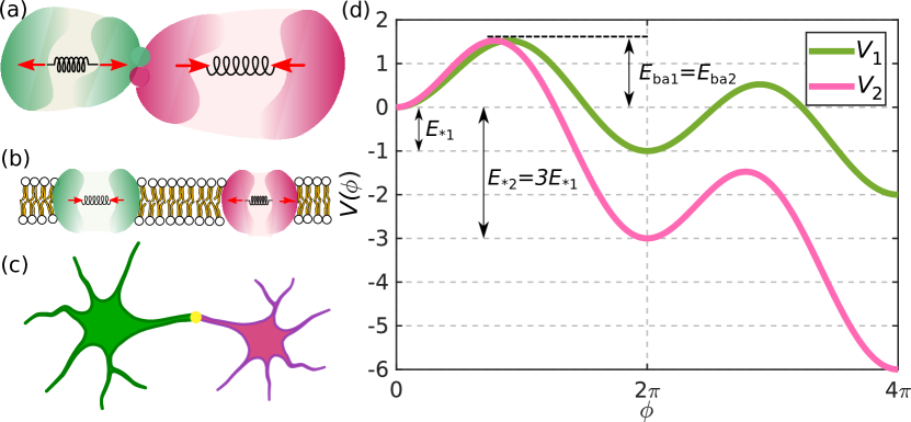
Figure 1: (a–c) Examples of coupled noise-activated oscillators: (a) Two enzymes attached to each other forming an oligomeric complex, (b) Two membrane channels interacting with each other via the intervening viscous medium, (c) Two excitable neurons interacting through a synapse. (d) The forces experienced by each oscillator can be represented using a tilted washboard potential, with a noise-activated oscillation corresponding to the phase $\phi$ advancing by the amount of $2\pi$ by crossing the energy barrier. In the case of enzymes, the potential represents the free energy of a (repeated) catalytic reaction.

Model

We consider two phases $\phi_{\alpha}$ with $\alpha=1,2$ that are coupled not through an interaction force or potential, but through the off-diagonal components of the mobility tensor that connects forces to velocities in the overdamped dynamics. That is, the phases evolve according to the following coupled Langevin equations

$$\dot{\phi}_{\alpha}=\sum_{\beta=1}^{2}\bigg{[}M_{\alpha\beta}\bigg{(}-\frac{\partial V_{\beta}(\phi_{\beta})}{\partial\phi_{\beta}}\bigg{)}+\sqrt{2k_{B}T}\Sigma_{\alpha\beta}\xi_{\beta}\bigg{]},$$ (1)

where $M_{\alpha\beta}$ is the mobility tensor, described below, $\Sigma_{\alpha\beta}$ is the principal square root of $M_{\alpha\beta}$ such that $M_{\alpha\beta}=\Sigma_{\alpha\gamma}\Sigma_{\beta\gamma}$, and $\xi_{\alpha}(t)$ is a Gaussian white noise satisfying $\langle\xi_{\alpha}(t)\rangle=0$, $\langle\xi_{\alpha}(t)\xi_{\beta}(t^{\prime})\rangle=\delta_{\alpha\beta}\delta(t-t^{\prime})$. Moreover, $k_{B}$ is the Boltzmann constant and $T$ is the temperature of the medium, so that $k_{B}T$ is the thermal energy controlling the strength of thermal fluctuations. For non-thermal systems, $k_{B}T$ may be taken as the strength of the effective noise. For the dynamics to be thermodynamically consistent, the mobility tensor must be symmetric and positive definite [36, 37]. We take the components of the mobility tensor to be $M_{11}=\mu_{1}$, $M_{22}=\mu_{2}$, and $M_{12}=M_{21}=\sqrt{\mu_{1}\mu_{2}}h$. Thus, the dimensionless parameter $h$ controls the strength of the coupling, and the condition of positive definiteness implies that it is constrained to the range $-1<h<1$. Through $\Sigma_{\alpha\beta}$, the mobility tensor also controls the form of the additive noise, so that the fluctuation-dissipation theorem is satisfied. This further implies that, independently of the strength of the coupling, the system is guaranteed to equilibrate to the Boltzmann distribution $P_{\mathrm{eq}}(\phi_{1},\phi_{2})\propto\exp(-[V_{1}(\phi_{1})+V_{2}(\phi_{2})]/k_{B}T)$ when such an equilibrium is possible (e.g. in the absence of nonequilibrium driving forces, $E_{*1}=E_{*2}=0$).

A coupling of the form in (1) arises naturally in processes that are coupled to each other through mechanical interactions at the nano- and microscale, as these are mediated by viscous, overdamped fields described by low Reynolds number hydrodynamics [37]. It represents a form of dissipative coupling, as it can be understood as arising from taking the overdamped limit of full Langevin dynamics in the presence of a friction force on phase $\phi_{\alpha}$ going as $f_{\alpha}=-\sum_{\beta=1}^{2}Z_{\alpha\beta}\dot{\phi}_{\beta}$, where $Z\equiv M^{-1}$ is a friction tensor. While in general the mobility tensor may be phase-dependent [20], for simplicity we focus here on the case of a constant mobility tensor [22].

The potentials are chosen to be tilted washboard potentials of the form $V_{\beta}(\phi_{\beta})=-F_{\beta}\phi_{\beta}-v_{\beta}\cos(\phi_{\beta}+\delta_{\beta})$, where the shift $\delta_{\beta}=\arcsin(F_{\beta}/v_{\beta})$ ensures that the minima of the potential are located at multiples of $2\pi$ and does not otherwise affect the phase dynamics. The maxima of the potential are located at $\phi_{\beta}^{\mathrm{max}}\equiv\pi-\arcsin(F_{\beta}/v_{\beta})$ (mod $2\pi$). The parameters $F_{\beta}$ and $v_{\beta}$ can be mapped to the energy barrier and the energy released per step [Fig. 1(d)] as $E_{\mathrm{ba}\beta}=[2\sqrt{1-(F_{\beta}/v_{\beta})^{2}}-(F_{\beta}/v_{\beta})(\pi-2\delta_{\beta})]v_{\beta}$ and $E_{*\beta}=2\pi F_{\beta}$. Therefore, in this minimal model we have eight parameters, namely $E_{\mathrm{ba1}}$, $E_{\mathrm{ba2}}$, $E_{*1}$, $E_{*2}$, $\mu_{1}$, $\mu_{2}$, $h$, and $k_{B}T$. Choosing a mobility scale $\mu_{0}$ and an energy scale $E_{0}$, which together define a timescale $(\mu_{0}E_{0})^{-1}$, these may be reduced to six dimensionless parameters. In the following, except where noted, we focus on the case of equal self-mobilities $\mu_{1}=\mu_{2}=\mu$, equal energy barriers $E_{\mathrm{ba1}}=E_{\mathrm{ba2}}=E_{\mathrm{ba}}$, and strongly driven dynamics $E_{*1}\gg E_{\mathrm{ba}}$ (we fix $E_{\mathrm{ba}}/E_{*1}=3\cdot 10^{-4}$). Thus, only three dimensionless parameters remain: $E_{*2}/E_{*1}$, which governs the asymmetry in the nonequilibrium driving of the two processes and we take to be $\geq 1$ (i.e. oscillator 2 is more strongly driven than oscillator 1); $h$, which defines the strength of the dissipative coupling; and $k_{B}T/{E_{\mathrm{ba}}}$, which defines the strength of the noise.

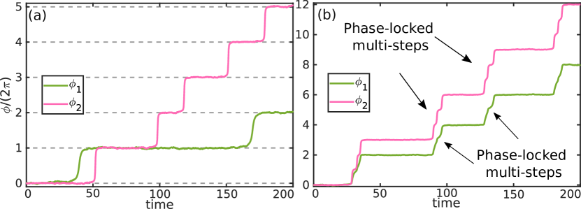
Figure 2: Examples of stochastic trajectories for asymmetry $E_{*2}/E_{*1}=5$ and noise strength $k_{B}T/E_{\mathrm{ba}}=1$. (a) In the absence of coupling, $h=0$, only a few, independent single steps are observed. (b) With coupling, $h=0.33$, a much larger overall number of steps is observed in the same time period, and moreover both phases move in tandem, in phase-locked, multi-step bursts. Time is given in units of $(\mu v_{1})^{-1}$.

Results

Stochastic trajectories

We briefly present the phenomenology observed in stochastic simulations of the equations of motion, (1), when the dissipative coupling is switched on (Fig. 2). In the absence of coupling, as expected, the trajectories are independent, and consist of single steps representing noise-activated crossings of the energy barriers in the potential, separated by long periods of time in which the phases are resting at the minima of the potential [see Fig. 1(d)]. With sufficiently large positive coupling, on the other hand, we observe that when the system is pushed out of the resting state, both oscillators advance at the same time, and moreover multiple steps occur as a result of a single fluctuation. This results in an overall enhanced average speed of the oscillators. In contrast to what was observed for identical oscillators [20, 22], the oscillators here do not appear to be synchronized, but there are signatures of phase locking, where $\phi_{1}$ advances $n_{1}$ steps while $\phi_{2}$ advances $n_{2}$ steps with a reproducible ratio $n_{1}:n_{2}$, in this example 2:3.

Importantly, this behavior is apparent even at very low values of the noise. This suggests that, as in the case of identical oscillators [20, 22], the phase locking phenomenology may be a consequence of bifurcations occurring in the underlying deterministic dynamical system.

Finite phase locking

We start by analyzing the phase portraits in $(\phi_{1},\phi_{2})$ space corresponding to the the deterministic part of (1). Because the dynamics are $2\pi$-periodic, this dynamical system is defined on the torus. Notice that the system always has four fixed points: a stable fixed point at (0,0), corresponding to both oscillators being at a minimum of their potential energy; an unstable fixed point, at $(\phi_{1}^{\mathrm{max}},\phi_{2}^{\mathrm{max}})$ when both at are a maximum; and two saddle points at $(\phi_{1}^{\mathrm{max}},0)$ and $(0,\phi_{2}^{\mathrm{max}})$, when one oscillator is at a minimum and the other at a maximum. Because of the structure of (1), the location and character of these fixed points is independent of the strength of the coupling. In particular, this means that local bifurcations (where fixed points split or merge and change character) are impossible. Any bifurcation in this system must be global, arising from a change in topology of the network of heteroclinic and homoclinic orbits connecting these four fixed points [38].

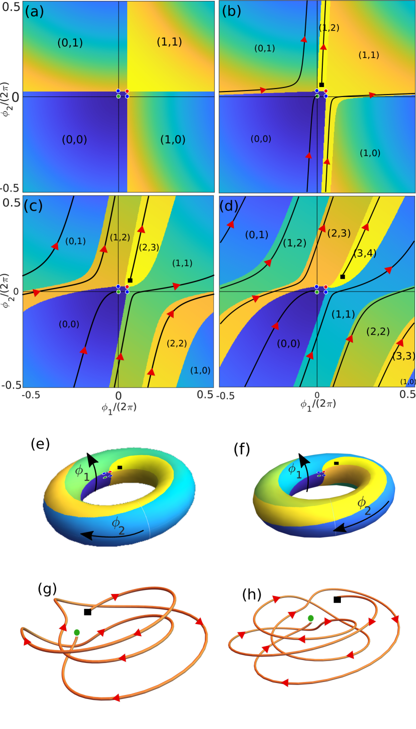
Figure 3: Phase portraits of the deterministic dynamics for weak asymmetry $E_{*2}/E_{*1}=5$ and various values of the coupling $h$. (a) $(1,1)$ topology for $h=0$. (b) $(1,2)$ topology for $h=0.05$. (c) $(2,3)$ topology for $h=0.19$. (d) $(3,4)$ topology for $h=0.33$. In all panels the green, red, and blue circles respectively correspond to the stable, unstable, and saddle fixed points of the dynamics. An example trajectory, starting at the black square and finishing at the stable fixed point, is shown in (b)–(d). The phase portraits in (c,d) are represented on the torus in (e,f). The example trajectories in (c,d) are represented as three-dimensional trajectories around the torus in (g,h). The colormap in (a)–(f) and the labels $(m,n)$ in (a)–(d) are explained in the text.

Phase portraits for weak driving force asymmetry $E_{*2}/E_{*1}=5$ and several values of the coupling $h$ are shown in Fig. 3. The labels $(m,n)$ are winding number pairs, describing how many times a trajectory starting in that region will wind around the torus along each dimension before reaching the stable fixed point. Equivalently, if the torus were to be unwrapped and tiled onto the plane, the stable fixed point reached when starting from that region in the phase portrait would be located at $(\phi_{1},\phi_{2})=(2\pi m,2\pi n)$. In the same vein, every point of the phase portrait (except those at heteroclinic orbits, which connect the unstable fixed point to the saddle points) has been colored according to the Euclidean distance between the point in question and the fixed point (for an unwrapped torus) that a trajectory starting at that point would reach. Thus, yellow corresponds to longer trajectories towards the fixed point, whereas blue corresponds to shorter trajectories.

In the planar phase portraits [Fig. 3(a)–(d)], regions with different winding number appear separated from each other by the heteroclinic orbits. However, on the surface of the torus [Fig. 3(e)–(f)], one can appreciate that the region enclosed by the heteroclinic orbits is still simply connected, covers the whole torus, and corresponds to the basin of attraction of the stable fixed point. With increasing coupling, we observe a series of global bifurcations in the heteroclinic network, which change the maximal winding numbers that are possible from e.g. (1,1) in the absence of coupling [Fig. 3(a)] to (3,4) for coupling $h=0.33$ [Fig. 3(d)]. This higher winding implies that the basin of attraction becomes a narrower and narrower strip, which winds around the torus an increasing number of times given by the highest winding number pair.

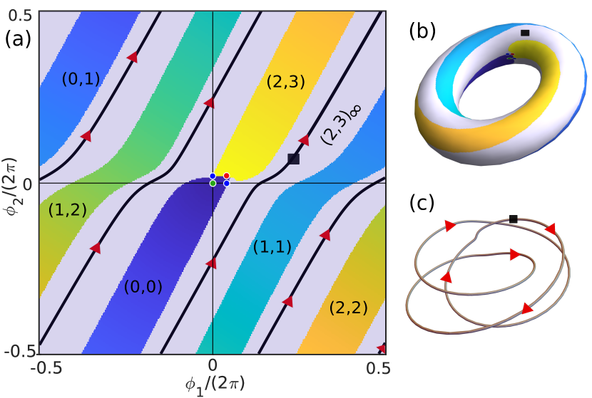
Figure 4: (a) Phase portrait for strong asymmetry $E_{*2}/E_{*1}=19.15$ and $h=0.51$, demonstrating a $(2,3)_{\infty}$ TPL state, and (b) its projection on a torus. The running band is shown in gray. The black line crossing through the black square (shown as a reference point) is an example of a periodic orbit within the running band, and is depicted in (c) as a three-dimensional loop around the torus, which forms a trefoil knot.

These bifurcations are responsible for the phenomenology observed in the stochastic simulations of Fig. 2, which we term finite phase locking. Indeed, let us take the phase portraits in Fig. 3(a,d) as an example. In the presence of fluctuations, a system initially located at the stable fixed point will typically be kicked by noise over either of the saddle points. In the absence of coupling, Fig. 3(a), this implies that the system enters either the (1,0) or the (0,1) basin, so that just one of the oscillators undergoes a single step. With coupling, Fig. 3(d), the system instead enters the (2,3) or the (1,1) basin, resulting in a finite number of steps taken in tandem by the two enzymes. Note that, typically, one of the two saddle points will be more easily reachable and thus traversed much more frequently than the other [39, 40]. It is also important to note that, although the maximal winding number pair in Fig. 3(d) is (3,4), observing a (3,4) transition in the stochastic system should be rare, as the system will typically escape the stable fixed point through one of the saddle points, and not through the unstable point. In this particular case, the stochastic simulations in Fig. 2(b) confirm that the $(0,\phi_{2}^{\mathrm{max}})$ saddle point is preferred, as all the stochastic transitions observed lead to a (2,3) transition. The time-course of a (2,3) stochastic transition is shown on top of the corresponding deterministic phase portrait in Movie S1.

Topological phase locking

For sufficiently strong driving force asymmetry, at specific values of the parameters belonging to a subset of codimension 1 in parameter space, we find phase portraits that are qualitatively different, see Fig. 4. The topology of the heteroclinic network changes, resulting in the formation of two homoclinic orbits that connect each of the two saddle points to itself. As a consequence, the phase space becomes disconnected into two regions: the basin of attraction of the stable fixed point, and a band of periodic orbits (in grey in Fig. 4). We refer to this phenomenon as topological phase locking (TPL).

Importantly, a nontrivial winding number pair can also be assigned to the running band region. In the particular example of Fig. 4, we observe that a periodic orbit (and, by extension, the running band region as a whole) winds two times along the $\phi_{1}$ direction and three times along the $\phi_{2}$ direction before closing in on itself, implying a winding number pair which we denote as $(2,3)_{\infty}$ in analogy with the notation for winding number pairs introduced above, where the $\infty$ subscript indicates that the trajectories are periodic and never reach a fixed point.

An example of a periodic trajectory within the running band is shown in Fig. 4(a), with the three-dimensional view of its projection on a torus shown in Fig. 4(c). It is interesting to note that the loop formed by the trajectory corresponds to a trefoil knot which, naturally, belongs to the class of torus knots (knots that lie on the surface of a torus) [32].

TPL has very strong consequences in the stochastic dynamics. In the presence of fluctuations, a system initially located at the stable fixed point will now be kicked by noise over either of the saddle points and fall into the running band. The phases $\phi_{1}$ and $\phi_{2}$ will then advance deterministically, in the ratio given by the corresponding winding number pair, until a sufficiently strong fluctuation kicks the system out of the running band and back into the stable fixed point. The average speed of the oscillations can therefore be greatly enhanced by the presence of a running band. The time-course of a stochastic multi-step run in a $(2,3)_{\infty}$ TPL state is shown on top of the corresponding deterministic phase portrait in Movie S2.

Phase-locking diagram

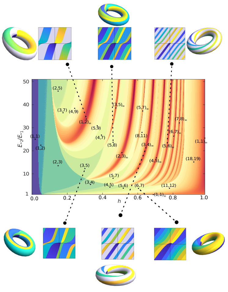
Figure 5: Phase-locking diagram as a function of the coupling strength $h$ and the driving force asymmetry $E_{*2}/E_{*1}$. The logarithmic colormap indicates the maximum winding of the second oscillator, and is used to differentiate the different phase portrait topologies that emerge. The labels indicate the topology in the region marked by the black dots. Selected examples of phase portraits are shown on a two-dimensional projection and on the torus.

To understand how and where these different phase portrait topologies emerge in parameter space, as well as the global bifurcations that connect them, we scanned the parameter space as a function of driving force asymmetry $E_{*2}/E_{*1}$ and coupling strength $h$. The topologies of phase portraits with finite phase locking were identified by means of the highest winding number pair $(m,n)$, whereas those corresponding to TPL were identified using the winding number pair $(m,n)_{\infty}$ of their running band.

The resulting phase-locking diagram, shown in Fig. 5, demonstrates an incredibly rich structure of bifurcations in the system. Note that the colors in the diagram correspond to the logarithmic value of the second number $n$ in the winding number pair $(m,n)$, with blue corresponding to low numbers and red to high numbers. We find a variety of regions corresponding to phase portraits with finite phase locking with different winding numbers. Most interestingly, however, we observe a number of dark red branches or resonances at which the winding numbers very sharply peak as we vary $E_{*2}/E_{*1}$ and/or $h$ and cross through the resonance. At the very center of these resonances, in a lower-dimensional manifold of codimension 1, we find the phase portraits with TPL (TPL states).

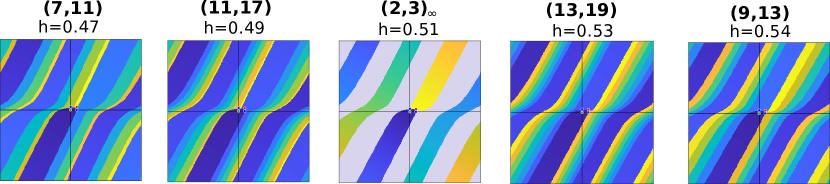
Figure S1: Phase portraits as the system crosses through the $(2,3)_{\infty}$ TPL state with increasing $h$. The driving force asymmetry is $E_{*2}/E_{*1}=19.15$. In all cases, $E_{\mathrm{ba1}}/E_{*1}=3\cdot 10^{-4}$.

To better understand the bifurcation structure, let us focus on the $(1,2)_{\infty}$ TPL state, which is the first one to appear as the coupling $h$ is increased. Suppose we begin at the dot marked $(2,5)$ to the left of the TPL state in Fig. 5, which corresponds to finite phase locking. As we increase $h$, we first observe a bifurcation to $(3,7)$, i.e. the maximal winding numbers increase by $(1,2)$. With a further increase of $h$, we observe a bifurcation to $(4,9)$, again by an increment of $(1,2)$. As we increase $h$ further, we keep undergoing more and more of these bifurcations, effectively climbing up an infinite ladder of the form $(2,5)+n\times(1,2)$ with $n=0,1,2,...,\infty$. After only a finite increase in $h$ up to a critical value $h_{\infty}$, the system has undergone an infinite number of these bifurcations and reaches a TPL state $\lim_{n\to\infty}[(2,5)+n\times(1,2)]=(1,2)_{\infty}$, i.e. a phase portrait with running band emerges. When $h$ is further increased beyond $h_{\infty}$, we now descend down a different infinite ladder, out of step with the first one, of the form $(4,7)+n\times(1,2)$ with $n=\infty,...,2,1,0$. The system thus ultimately reaches the finite phase locking topology $(4,7)$. A further increase of $h$ now takes us into the range of influence of the $(3,5)_{\infty}$ TPL state, so that the system begins to climb up a new ladder and bifurcates to a $(4,7)+(3,5)=(7,12)$ topology, and so on and so forth. An example of how the phase portraits change as one moves across the $(2,3)_{\infty}$ TPL state is shown in SI Fig. S1.

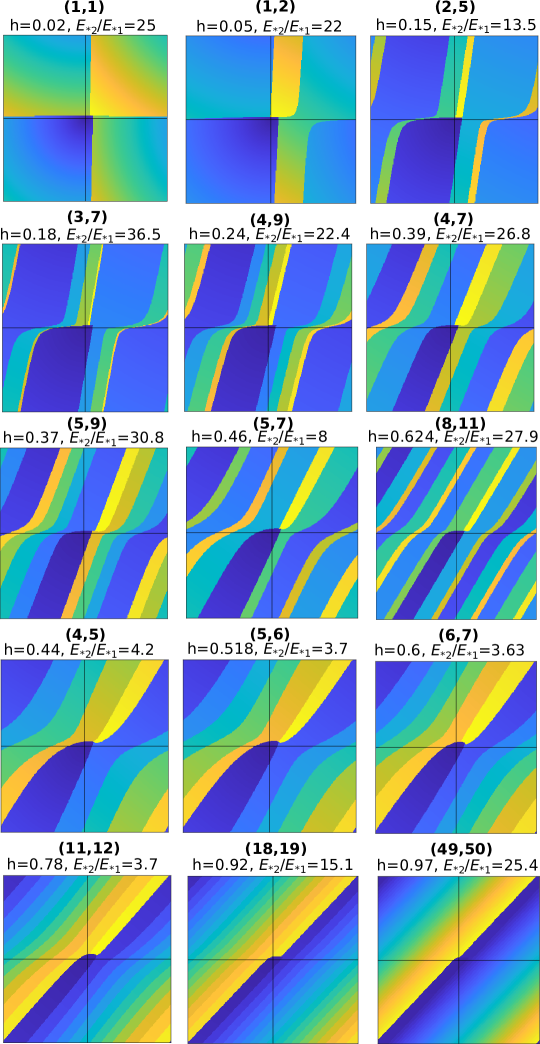
Figure S2: Various phase portraits with finite phase locking. In all cases, $E_{\mathrm{ba1}}/E_{*1}=3\cdot 10^{-4}$.

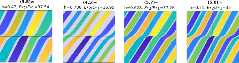
Figure S3: Various TPL phase portraits. For the topologies $(3,5)_{\infty},(4,5)_{\infty}$ and $(5,7)_{\infty}$, we used $E_{\mathrm{ba1}}/E_{*1}=3\cdot 10^{-4}$. For the portrait $(5,8)_{\infty}$, we used $E_{\mathrm{ba1}}/E_{*1}=1\cdot 10^{-4}$.

A number of phase portraits for different points on the phase-locking diagram is shown in the insets of Fig. 5, and more examples are shown in SI Fig. S2 and SI Fig. S3. In particular, a number of phase portraits displaying TPL are included. Just like the $(2,3)_{\infty}$ trajectory in Fig. 4, periodic trajectories inside these running bands form torus knots. Such knots are defined by a tuple $(q,p)$ where $q,p$ are coprime to each other and characterize the winding along the two axis of the torus [32]. For all $(m,n)_{\infty}$ topologies that we have observed, $m$ and $n$ were indeed coprime, suggesting that the TPL states correspond to various torus knots. Torus-knot trajectories have been found in the past in soliton equations, for instance in the non-linear Schrödinger equation [41]. Our system provides a new example of a non-linear dynamical system which can give rise to such mathematical structures.

The phase-locking diagram in Fig. 5 bears some resemblance to the well-known Arnold tongues describing phase locking in a number of other systems [2, 7, 8, 9]. However, the resemblance is only superficial: in fact, while in the case of Arnold tongues the key parameter controlling phase-locking ratios is the frequency asymmetry and the coupling merely acts to broaden the phase-locking regions, here the opposite is true. The main parameter controlling the phase-locking ratios is the coupling $h$, and the very limited amount of broadening of the phase-locking regions originates from the driving asymmetry $E_{*2}/E_{*1}$. Besides this clear operational difference, the context here is entirely different, as we are still dealing with noise-activated dynamics – although the coexistence of a running band and a stable fixed point leads to a coexistence of dissipative and effectively conservative/deterministic dynamics [23].

Lastly, it is worth commenting on the role of symmetry. Interestingly, the TPL state $(1,1)_{\infty}$ occurs in two very particular lower dimensional manifolds, namely on the manifold defined by $E_{*2}/E_{*1}=1$ and $h>h_{*}$, and on the manifold defined by $h=1$ (maximum coupling allowed by positive-definiteness of the mobility matrix). This explains the results of Ref. 20 and Ref. 22, which dealt with symmetric oscillators and observed $(1,1)_{\infty}$ topologies for all values of the coupling above a critical value $h_{*}$. This appears to be a special feature of the symmetric case, as in the general case studied here we find that TPL states only occur at discrete values of the coupling strength.

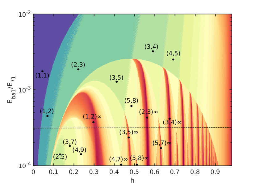
Figure S4: Phase-locking diagram as a function of coupling strength $h$ and $E_{\mathrm{ba1}}/E_{*1}$, for fixed $E_{\mathrm{ba2}}/E_{\mathrm{ba1}}=1$ and $E_{*2}/E_{*1}=35$. The horizontal line corresponds to $E_{\mathrm{ba1}}/E_{*1}=3\cdot 10^{-4}$ which was used throughout the main text.

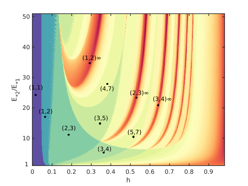
Figure S5: Phase-locking diagram as a function of the coupling strength $h$ and the driving force asymmetry $E_{*2}/E_{*1}$. In comparison with Fig. 5 in the main text, which used $E_{\mathrm{ba1}}/E_{*1}=3\cdot 10^{-4}$ and $E_{\mathrm{ba2}}/E_{\mathrm{ba1}}=1$, here we use $E_{\mathrm{ba1}}/E_{*1}=10^{-3}$ and $E_{\mathrm{ba2}}/E_{\mathrm{ba1}}=0.5$.

For the sake of completeness, we have calculated analogous phase-locking diagrams for other choices of system parameters, see SI Fig. S4 and SI Fig. S5. The overall qualitative features are unchanged.

Signatures of TPL in the stochastic dynamics

In order to ascertain whether the TPL states in Fig. 5 have an effect on the stochastic dynamics in the presence of noise, we now quantify the long-time behavior of our stochastic simulations. In particular, we will measure the average speed $\Omega_{\alpha}$ and diffusion coefficient $D_{\alpha}$ of each oscillator ($\alpha=1,2$), and the correlation $C$ between the two oscillators. Defining $\delta\phi_{\alpha}(\tau;t)\equiv\phi_{\alpha}(t+\tau)-\phi_{\alpha}(t)$, we calculate the average speed of oscillator $\alpha$ as

$$\langle\delta\phi_{\alpha}(\tau;t)\rangle_{t}~{}\mathop{\sim}_{\tau\to\infty}~{}\Omega_{\alpha}\tau,$$ (2)

where the operator $\langle...\rangle_{t}$ denotes a time average over a long simulation. The diffusion coefficient is similarly calculated as

$$\langle[\delta\phi_{\alpha}(\tau;t)-\langle\delta\phi_{\alpha}(\tau;t)\rangle_{t}]^{2}\rangle_{t}{~{}\underset{\tau\to\infty}{\sim}~{}}2D_{\alpha}\tau.$$ (3)

Finally, the correlation between oscillators is calculated as

$$\frac{\langle\prod_{\alpha=1,2}[\delta\phi_{\alpha}(\tau;t)-\langle\delta\phi_{\alpha}(\tau;t)\rangle_{t}]\rangle_{t}}{\sqrt{\prod_{\alpha=1,2}\langle[\delta\phi_{\alpha}(\tau;t)-\langle\delta\phi_{\alpha}(\tau;t)\rangle_{t}]^{2}\rangle_{t}}}~{}\underset{\tau\to\infty}{\sim}~{}C,$$ (4)

and is bounded between $-1$ and $1$ for perfectly anticorrelated and perfectly correlated processes, respectively.

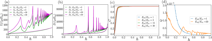
Figure 6: Signatures of TPL states in the stochastic simulations, appearing as a function of the coupling strength $h$. (a) Average speed and (b) diffusion coefficient of the oscillators for weak and strong driving force asymmetry. Peaks are observed as the resonances are crossed for strong asymmetry. (c) The correlation between oscillators rapidly grows independently of the driving force asymmetry. (d) Quality factor quantifying the stochastic thermodynamics of precision (Eq. 5). The quality factor drops as the resonances are crossed.

We first considered the average speed $\Omega_{\alpha}$ as a function of coupling strength for fixed values of the driving asymmetry [Fig. 6(a)], corresponding to horizontal cuts in the phase-locking diagram of Fig. 5. For small asymmetry, where there are no TPL states, the average speed of both oscillators increases monotonically with increasing coupling. The phenomenology is very different for strong asymmetry, where increasing the coupling strength takes the system through a series of TPL states. At each of these, we find that the average speed of the coupled slow-fast oscillators sharply peaks. Thus, the presence of a running band strongly enhances the average speed of the oscillators.

An analogous behavior is observed for the diffusion coefficients $D_{\alpha}$, with a monotonic increase in the absence of TPL states at weak driving force asymmetry, and very sharp peaks when TPL states are crossed at strong driving force asymmetry [Fig. 6(b)]. In analogy with the standard giant diffusion observed for single oscillators at the threshold of noise-activated and deterministic dynamics [33], the giant diffusion for TPL states can be understood as a consequence of the bistability that arises in systems with a running band, which stochastically switch between dissipative dynamics that keep the system at the stable fixed point, and quasi-deterministic dynamics when the system is within the running band [22].

We also note that, independently of the amount of driving force asymmetry, the correlation $C$ quickly grows with increasing coupling, and for $h\gtrsim 0.1$ saturates to $C\approx 1$ indicating perfect correlation between the oscillators, see Fig. 6(c). Indeed, from the topology of the deterministic phase portraits, we expect the dynamics of the oscillators to become correlated for any topology other than the trivial topology (1,1), which is present only at very low $h$ independently of the driving force asymmetry.

Stochastic thermodynamics of precision

Lastly, we consider the stochastic thermodynamics of the two coupled processes [42]. In particular, the thermodynamic uncertainty relation (TUR) [34] shows that energy dissipation (or entropy production) puts a fundamental lower bound to the precision of a nonequilibrium process. More precisely, the multidimensional TUR (MTUR) provides the bound $\bm{\mathcal{J}}^{T}\bm{\mathcal{D}}^{-1}\bm{\mathcal{J}}\leq\dot{\sigma}/k_{B}$ at steady state, where $\dot{\sigma}$ is the entropy production rate, $\bm{\mathcal{J}}$ is any vectorial current, and $\bm{\mathcal{D}}$ is the diffusion matrix describing the fluctuations of the current [35].

In our two-oscillator system, we have $\mathcal{J}_{\alpha}=\Omega_{\alpha}$ and $\mathcal{D}_{\alpha\alpha}=D_{\alpha}$ for $\alpha=1,2$, as well as $\mathcal{D}_{12}=\mathcal{D}_{21}=C\sqrt{D_{1}D_{2}}$. The MTUR can then be rewritten explicitly as

$$Q\equiv\frac{1}{1-C^{2}}\bigg{(}\frac{\Omega_{1}^{2}}{D_{1}}-\frac{2C\Omega_{1}\Omega_{2}}{\sqrt{D_{1}D_{2}}}+\frac{\Omega_{2}^{2}}{D_{2}}\bigg{)}\frac{k_{B}}{\dot{\sigma}}\leq 1$$ (5)

where $Q$ is a quality factor, equal to 1 when the bound is saturated (the precision is as high as thermodynamically allowed) and 0 for a purely diffusive process. The entropy production $\dot{\sigma}$ can be calculated from the steady state dissipation $\dot{\sigma}T=F_{1}\Omega_{1}+F_{2}\Omega_{2}$.

The behavior of the quality factor $Q$ as a function of the coupling strength $h$ for both weak and strong driving force asymmetries is shown in Fig. 6(d). The fact that for strong asymmetry the system crosses through various TPL states with increasing $h$ is clearly signalled in the stochastic thermodynamics of precision. In particular, we see that $Q$ strongly decreases at each TPL state, which may be counter-intuitive considering that the average speed peaks at these states [Fig. 6(a)]. However, note that the diffusion coefficient also strongly peaks at the TPL states [Fig. 6(b)], more sharply than the average speed, so that the quality factor ultimately decreases at the TPL states.

Discussion

We have studied a minimal model of two non-identical noise-activated oscillators that interact with each other through a dissipative coupling. Such a coupling is distinct from more commonly-employed Kuramoto-style couplings in theoretical studies of synchronization, and is of direct relevance to a number of physical systems ranging from biological enzymes and molecular motors to optomechanical devices, superconducting Josephson junctions, and more.

From the dynamical systems perspective, in the absence of noise, we found that the parameter space of this minimal model displays a surprisingly rich structure (Fig. 5), including a complex hierarchy of global bifurcations that culminate in special phase-locked states which we term topologically phase-locked (TPL). In the TPL states, the phase space splits into two disconnected regions: the basin of attraction of the stable fixed point, which displays dissipative dynamics; and a band of periodic orbits in the shape of a torus knot (defined by two coprime integer winding numbers) in which effectively conservative dynamics are observed, with both oscillators advancing in rational multiples of each other, as given by the ratio of winding numbers. The emergence of TPL states has a strong effect in the stochastic dynamics, and in particular leads to a giant enhancement of both the average velocity and the diffusion coefficient of the oscillators.

Besides the obvious interest from the point of view of dynamical systems theory, we anticipate that our results may find practical applications in a variety of systems. In particular, we previously showed how a dissipative coupling arises when two enzymes that undergo conformational changes during their chemical reactions are in proximity of, or mechanically linked to, each other. We hypothesize that the rate enhancements afforded by TPL states could be exploited by enzymes that form heterodimers (that is, complexes of two distinct enzymes) in order to boost the catalytic activity of the slower enzyme. Indeed, some heterodimeric enzymes show higher activity than what could be achieved by the two individual enzymes alone [43, 44]. Alternatively, TPL states may be targeted in engineered systems whose dissipative coupling and driving force asymmetry can be experimentally controlled, such as superconducting Josephson junction arrays [23, 24], laser cavities [25, 26] or optomechanical devices [27, 28]. composed.

I Methods

Stochastic simulations

To integrate the stochastic differential equations, Eq. 1, we employed the Euler-Maruyama method using a custom code written in the Julia language [45]. Time was nondimensionalized as $\tilde{t}=\mu_{1}v_{1}t$. For the results in Fig. 6, a time step $d\tilde{t}=10^{-2}$ was used, with the total number of steps equal to $10^{9}$ and the number of samples equal to $10^{6}$. We also averaged over 10 different runs. More detailed information on how the observables in Eqs. 2–4 were calculated can be found in the supplementary information of Ref. 22.

Phase portraits

To generate phase portraits, we integrated the deterministic equations of motion (corresponding to Eq. 1 without the noise term) using the built-in ode45 integrator in MATLAB [46], which employs a 4th order Runge-Kutta method. A $301\times 301$ grid of initial points in the interval $-\pi<\phi_{1,2}<\pi$ was used, and we integrated the trajectories up to a maximum integration time $\tilde{t}_{\mathrm{max}}=100$. The final points were then used to identify the winding number $(m,n)$ if the trajectory reached a stable fixed point, or $(m,n)_{\infty}$ if the trajectory was found to be periodic and thus to lie on a running band.

II Supplementary Information

We provide the following movies:

• Movie 1:An example of a stochastic $(2,3)$ transition in a $(3,4)$ finite phase locking topology. On the left panel, the evolution of the trajectory is shown on top of the phase portrait. On the right panel, the completed cycles are shown as a function of simulation time.

• Movie 2: An example of the stochastic dynamics on a $(2,3)_{\infty}$ TPL topology. On the left panel, the evolution of the trajectory is shown on top of the phase portrait. On the right panel, the completed cycles are shown as a function of simulation time.