NeuroCUT: A Neural Approach for Robust Graph Partitioning

Abstract.

Graph partitioning aims to divide a graph into $k$ disjoint subsets while optimizing a specific partitioning objective. The majority of formulations related to graph partitioning exhibit NP-hardness due to their combinatorial nature. Conventional methods, like approximation algorithms or heuristics, are designed for distinct partitioning objectives and fail to achieve generalization across other important partitioning objectives. Recently machine learning-based methods have been developed that learn directly from data. Further, these methods have a distinct advantage of utilizing node features that carry additional information. However, these methods assume differentiability of target partitioning objective functions and cannot generalize for an unknown number of partitions, i.e., they assume the number of partitions is provided in advance. In this study, we develop NeuroCUT with two key innovations over previous methodologies. First, by leveraging a reinforcement learning-based framework over node representations derived from a graph neural network and positional features, NeuroCUT can accommodate any optimization objective, even those with non-differentiable functions. Second, we decouple the parameter space and the partition count making NeuroCUT inductive to any unseen number of partition, which is provided at query time. Through empirical evaluation, we demonstrate that NeuroCUT excels in identifying high-quality partitions, showcases strong generalization across a wide spectrum of partitioning objectives, and exhibits strong generalization to unseen partition count.

1. Introduction and Related Work

Graph partitioning is a fundamental problem in network analysis with numerous real-world applications in various domains such as system design in online social networks (Pujol et al., 2009), dynamic ride-sharing in transportation systems (Tafreshian and Masoud, 2020), VLSI design (Kahng et al., 2011), and preventing cascading failure in power grids (Li et al., 2005). The goal of graph partitioning is to divide a given graph into disjoint subsets where nodes within each subset exhibit strong internal connections while having limited connections with nodes in other subsets. Generally speaking, the aim is to find somewhat balanced partitions while minimizing the number of edges across partitions.

Several graph partitioning formulations have been studied in the literature, mostly in the form of discrete optimization (Karypis et al., 1997; Karypis and Kumar, 1998, 1999; Andersen et al., 2006; Chung, 2007). The majority of the formulations are NP-hard and thus the proposed solutions are either heuristics or algorithms with approximate solutions (Karypis et al., 1997). Recently, there have been attempts to solve graph partitioning problem via neural approaches. The neural approaches have a distinct advantage that they can utilize node features. Node features supply additional information and provide contextual insights that may improve the accuracy of graph partitioning. For instance, (Wang et al., 2017) has recognized the importance of incorporating node attributes in graph clustering where nodes are partitioned into disjoint groups. Note that there are existing neural approaches (Khalil et al., 2017; Manchanda et al., 2020; Kool et al., 2018; Joshi et al., 2019) to solve other NP-hard graph combinatorial problems (e.g., minimum vertex cover). However these methods are not generic enough to solve graph partitioning.

In this paper, we build a single framework to solve several graph partitioning problems. One of the most relevant to our work is the method DMoN by Tsitsulin et al. (2023a). This method designs a neural architecture for cluster assignments and use a modularity-based objective function for optimizing these assignments. Another method, that is relevant to our work is GAP, which is an unsupervised learning method to solve the balanced graph partitioning problem (Nazi et al., 2019). It proposes a differentiable loss function for partitioning based on a continuous relaxation of the normalized cut formulation. Deep-MinCut being an unsupervised approach learns both node embeddings and the community structures simultaneously where the objective is to minimize the mincut loss (Duong et al., 2023). Another method solves the multicut problem where the number of partitions is not an input to the problem (Jung and Keuper, 2022). The idea is to construct a reformulation of the multicut ILP constraints to a polynomial program as a loss function. However, the problem formulation is different than the generic normalized cut or mincut problem. Finally,  (Gatti et al., 2022) solves the normalized cut problem only for the case where the number of partitions is exactly two. Nevertheless, these neural approaches for the graph partitioning problem often do not use node features and only limited to a distinct partitioning objective. Here, we point out notable drawbacks that we address in our framework.

• Non-inductivity to partition count: The number of partitions required to segment a graph is an input parameter. Hence, it is important for a learned model to generalize to any partition count without retraining. Existing neural approaches are non-inductive to the number of partitions, i.e they can only infer on number of partitions on which they are trained. Additionally, it is worth noting that the optimal number of partitions is often unknown beforehand. Hence, it is a common practice to experiment with different partition counts and evaluate their impact on the partitioning objective. While the existing methods (Tsitsulin et al., 2023a; Nazi et al., 2019; Gatti et al., 2022) assume that the number of partitions ($k$) is known beforehand, our proposed method can generalize to any $k$.

• Non-generalizability to different cut functions: Multiple objective functions for graph cut have been studied in the partitioning literature. The optimal objective function hinges upon the subsequent application in question. For instance, the two most relevant studies, DMoN (Tsitsulin et al., 2023a) and GAP (Nazi et al., 2019) focus on maximizing modularity and minimizing normalized cut respectively. Our framework is generic and can solve different partitioning objectives.

• Assumption of differential objective function: Existing neural approaches assume the objective function to be differentiable. As we illustrate in § 2, the assumption does not always hold in the real-world. For instance, the sparsest cut (Chawla et al., 2006) and balanced cut (Nazi et al., 2019) objectives are not differentiable.

1.1. Contributions:

In this paper, we circumvent the above-mentioned limitations through the following key contributions.

• Versatile objectives: We develop NeuroCUT; an auto-regressive, graph reinforcement learning framework that integrates positional information, to solve the graph partitioning problem for attributed graphs. Diverging from conventional algorithms, NeuroCUT can solve multiple partitioning objectives. Moreover, unlike other neural methods, NeuroCUT can accommodate diverse partitioning objectives, without the necessity for differentiability.

• Inductivity to number of partitions: The parameter space of NeuroCUT is independent of the partition count. This innovative decoupled architecture endows NeuroCUT with the ability to generalize effectively to arbitrary partition count specified during inference.

• Empirical Assessment: We perform comprehensive experiments employing real-world datasets, evaluating NeuroCUT across four distinct graph partitioning objectives. Our empirical investigation substantiates the efficacy of NeuroCUT in partitioning tasks, showcasing its robustness across a spectrum of objective functions. We also demonstrate the capacity of NeuroCUT to generalize effectively to partition sizes that it has not encountered during training.

2. Problem Formulation

In this section, we introduce the concepts central to our work and formulate the problem. All the notations used in this work are outlined in Table 1.

Definition 1 (Graph).

We denote a graph as $\mathcal{G}=(\mathcal{V},\mathcal{E},\textbf{{X}})$ where $\mathcal{V}$ is the set of nodes, $\mathcal{E}\subseteq\mathcal{V}\times\mathcal{V}$ is the set of edges and $\textbf{{X}}\in\mathbb{R}^{|\mathcal{V}|\times|F|}$ refers to node feature matrix where $F$ is the set of all features in graph $\mathcal{G}$.

Definition 2 (Cut).

A cut $\mathcal{C}=(\mathcal{S},\mathcal{T})$ is a partition of $\mathcal{V}$ into two subsets $\mathcal{S}$ and $\mathcal{T}$. The cut-set of $\mathcal{C}=(\mathcal{S},\mathcal{T})$ is the set $(u,v)\in\mathcal{E}|u\in\mathcal{S},v\in\mathcal{T}$ of edges that have one endpoint in $\mathcal{S}$ and the other endpoint in $\mathcal{T}$.

Definition 3 (Graph Partitioning).

Given graph $\mathcal{G}$, we aim to partition $\mathcal{G}$ into $k$ disjoint sets $\mathcal{P}=\{P_{1},P_{2},\cdots,P_{k}\}$ such that the union of the nodes in those sets is equal to $\mathcal{V}$ i.e $\cup_{i=1}^{k}P_{i}=\mathcal{V}$ and each node belongs to exactly one partition.

Partitioning Objective: We aim to minimize/maximize a partitioning objective of the form ${Obj}(\mathcal{G},\mathcal{P})$. A wide variety of objectives for graph partitioning have been proposed in the literature. Without loss of generality, we consider the following four objectives. These objectives are chosen due to being well studied in the literature, while also being diverse from each other.

1. $k$-MinCut (Saran and Vazirani, 1995): Partition a graph into $k$ partitions such that the total number of edges across partitions is minimized.

   (1) $$\text{$k$-mincut}(\mathcal{P})=\sum_{l=1}^{|\mathcal{P}|}\frac{|\operatorname{cut}\left(P_{l},\overline{P_{l}}\right)|}{\sum_{e\in\mathcal{E}}|e|}$$

   Here $P_{l}$ refers to the set of elements in $l^{th}$ partition of $\mathcal{P}$ as described in Def.  3 and $\overline{P_{l}}$ refers to set of elements not in $P_{l}$.

2. Normalized Cut (Shi and Malik, 2000): The $k$-MinCut criteria favors cutting small sets of isolated nodes in the graph. To avoid this unnatural bias for partitioning out small sets of points, normalised cut computes the cut cost as a fraction of the total edge connections to all the nodes in the graph.

   (2) $$\operatorname{Ncut}(\mathcal{\mathcal{P}}):=\sum_{l=1}^{|\mathcal{P}|}\frac{|\operatorname{cut}\left(P_{l},\overline{P_{l}}\right)|}{\operatorname{vol}\left(P_{l},\mathcal{V}\right)}$$

   Here, $\operatorname{vol}\left(P_{l},\mathcal{V}\right):=\sum_{v_{i}\in P_{l},v_{j}\in\mathcal{V}}e(v_{i},v_{j})$.

3. Balanced Cuts (Nazi et al., 2019): Balanced cut favours partitions of equal sizes so an extra term that indicates the squared distance from equal sized partition is added to normalised cuts.

   (3) $$\operatorname{Balanced-Cuts}(\mathcal{\mathcal{P}}):=\sum_{l=1}^{|\mathcal{P}|}\frac{|\operatorname{cut}\left(P_{l},\overline{P_{l}}\right)|}{\operatorname{vol}\left(P_{l},\mathcal{V}\right)}+\frac{(|P_{l}|-|\mathcal{V}|/k)^{2}}{|\mathcal{V}|^{2}}$$

   Here, $\operatorname{vol}\left(P_{l},\mathcal{V}\right):=\sum_{v_{i}\in P_{l},v_{j}\in\mathcal{V}}e(v_{i},v_{j})$

4. Sparsest Cuts (Chawla et al., 2006): Two-way sparsest cuts minimize the cut edges relative to the number of nodes in the smaller partition. We generalize it to $k$-way sparsest cuts by summing up the value for all the partitions. The intuition behind sparsest cuts is that any partition should neither be very large nor very small.

   (4) $$\phi(S,\bar{S}) =\frac{\operatorname{cut}(S,\bar{S})}{\min(|S|,|\bar{S}|)}$$

   (5) $$\operatorname{Sparsest-Cuts}(\mathcal{\mathcal{P}}) =\sum_{l=1}^{|\mathcal{P}|}\phi(P_{l},\overline{P_{l}})$$

Problem 1 (Learning to Partition Graph ).

Given a graph $\mathcal{G}$ and the number of partitions $k$, the goal is to find a partitioning $\mathcal{P}$ of the graph $\mathcal{G}$ that optimizes a target objective function ${Obj}(\mathcal{G},\mathcal{P})$. Towards this end, we aim to learn a policy $\pi$ that assigns each node $v\in\mathcal{V}$ to a partition in $\mathcal{P}$.

In addition to our primary goal of finding a partitioning that optimizes a certain objective function, we also desire policy $\pi$ to have the following properties:

1. Inductive: Policy $\pi$ is inductive if the parameters of the policy are independent of both the size of the graph and the number of partitions $k$. If the policy is not inductive then it will be unable to infer on unseen size graphs/number of partitions.

2. Learning Versatile Objectives: To optimize the parameters of the policy, a target objective function is required. The optimization objective may not be differentiable and it might not be always possible to obtain a differentiable formulation. Hence, the policy $\pi$ should be capable of learning to optimize for a target objective that may or may not be differentiable.

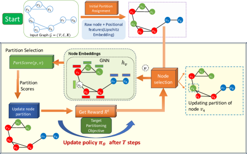
Figure 1. Architecture of NeuroCUT. First, the initial partitioning of the graph is performed based on node raw features and positional embeddings. These embeddings are refined using GNN to infuse toplogical information from neighborhood. At each step a node is selected and its partitioned is updated. During the training phase the GNN parameters are updated and hence embeddings are re-computed. During inference, the GNN is called only once to compute the embeddings of the nodes of the graph.

Symbol	Meaning
$\mathcal{G}$	Graph
$\mathcal{V}$	Node set
$e$	Edge $e\in\mathcal{E}$
$\mathcal{E}$	Edge set
X	Feature matrix containing raw node features
$\mathcal{N}_{v}$	Neighboring nodes of node $v$
$Obj(\mathcal{G},\mathcal{P})$	Objective function based upon graph $\mathcal{G}$ and its partitioning $\mathcal{P}$
$k$	Number of partitions
$\mathcal{P}^{t}$	Partitioning at time $t$
${P}^{t}_{i}$	$i^{th}$ partition at time $t$
$\overline{{P}_{i}}$	Set of nodes that are not in the $i^{th}$ partition
$\mathcal{S}^{t}$	State of system at step $t$
$\operatorname{PART}(\mathcal{P}^{t},v)$	Partition of node $v$ at time $t$
$\mathcal{S}^{t}$	State representation of Partitions and Graph at step $t$
$\mathbf{pos}(v)$	Positional embedding of node $v$
$\mathbf{emb_{init}}(v)$	Initial embedding of node $v$
$\alpha$	Number of anchor nodes for lipschitz embedding
$T$	Length of trajectory
$\pi$	Policy function

Table 1. Notations used in the paper

3. NeuroCUT: Proposed Methodology

Fig. 1 describes the framework of NeuroCUT. For a given input graph $\mathcal{G}$, we first construct the initial partitions of nodes using a clustering based approach. Subsequently, a message-passing Gnn embeds the nodes of the graph ensuring inductivity to different graph sizes. Next, the assignment of nodes to partitions proceeds in a two-phased strategy. We first select a node to change its partition and then we choose a suitable partition for the selected node. Further, to ensure inductivity on the number of partitions, we decouple the number of partitions from the direct output representations of the model. This decoupling allows us to query the model to an unseen number of partitions. After a node’s partition is updated, the reward with respect to change in partitioning objective value is computed and the parameters of the policy are optimized. The reward is learned through reinforcement learning (RL) (Sutton and Barto, 2018).

The choice of using RL is motivated through two observations. Firstly, cut problems on graphs are generally recognized as NP-hard, making it impractical to rely on ground-truth data, which would be computationally infeasible to obtain. Secondly, the cut objective may lack differentiability. Therefore, it becomes essential to adopt a learning paradigm that can be trained even under these non-differentiable constraints. In this context, RL effectively addresses both of these critical requirements. Additionally, in the process of sequentially constructing a solution, RL allows us to model the gain obtained by perturbing the partition of a node.

Markov Decision Process. Given a graph $\mathcal{G}$, our objective is to find the partitioning $\mathcal{P}$ that maximizes/minimizes the target objective function $Obj(\mathcal{G},\mathcal{P})$. We model the task of iteratively updating the partition for a node as a Markov Decision Process (MDP) defined by the tuple $(S,\mathcal{A},\rho,R,\gamma)$. Here, $S$ is the state space, $\mathcal{A}$ is the set of all possible actions, $\rho:S\times S\times\mathcal{A}\rightarrow[0,1]$ denotes the state transition probability function, $R:S\times\mathcal{A}\rightarrow\mathbb{R}$ denotes the reward function and $\gamma\in(0,1)$ the discounting factor. We next formalize each of these notions in our MDP formulation.

3.1. State: Initialization & Positional Encoding

Initialization. Instead of directly starting from empty partitions, we perform a warm start operation that clusters the nodes of the graph to obtain the initial graph partitions. The graph is clustered into $k$ clusters based on their raw features and positional embeddings (discussed below). We use K-means (MacQueen et al., 1967) algorithm for this task. The details of the clustering are present in Appendix A.2.

Positional Encoding (Embeddings). Given that the partitioning objectives are NP-hard mainly due to the combinatorial nature of the graph structure, we look for representations that capture the location of a node in the graph. Positional encodings provide an idea of the position in space of a given node within the graph. Two nodes that are closer in the graph, should be closer in the embedding space. Towards this, we use Lipschitz Embedding (Bourgain, 1985). Let $\mathcal{A}=\{a_{1},\cdots,a_{\alpha}\}\subseteq\mathcal{V}$ be a randomly selected subset of $\alpha$ nodes. We call them anchor nodes. From each anchor node $i$, the walker starts a random walk (Bianchini et al., 2005) and jumps to a neighboring node $j$ with a transition probability ($\mathbf{W}_{ij}$) governed by the transition probability matrix $\mathbf{W}\in\mathbb{R}^{|V|\times|V|}$. Furthermore, at each step, with probability $c$ the walker jumps to a neighboring node $j$ and returns to the node $i$ with $1-c$. Let $\vec{r}_{ij}$ corresponds to the probability of the random walker starting from node $i$ and reaching node $j$.

(6) $$\vec{r}_{i}=c\tilde{\mathbf{W}}\vec{r}_{i}+(1-c)\vec{e}_{i}$$

Eq. 6 describes the random walk starting at node $i$. In vector $\vec{e}_{i}\in\mathbb{R}^{|V|\times 1}$, only the $i^{th}$ element (the initial anchor node) is $1$, and the rest are set to zero. We set $\mathbf{W}_{ij}=\frac{1}{degree(j)}$ if edge $e_{ij}\in\mathcal{E}$, $0$ otherwise. The random walk with restart process is repeated for $\beta$ iterations, where $\beta$ is a hyper-parameter. Here $\vec{e}_{i}\in\mathbb{R}^{|V|\times 1}$ and $c$ is a scalar.

Based upon the obtained random walk vectors for the set of anchor nodes $\mathcal{A}$, we embed all nodes $u\in\mathcal{V}$ in a $\alpha$-dimensional feature space:

(7) $$\mathbf{pos}(u)=[r_{1u},r_{2u},\cdots,r_{\alpha u}]$$

To accommodate both raw feature and positional information we concatenate the raw node features i.e $\textbf{X}[u]$ with the positional embedding $\mathbf{pos}(u)$ for each node $u$ to obtain the initial embedding which will act as input to our neural model. Specifically,

(8) $$\mathbf{emb_{init}}(u)=\textbf{X}[u]\;\;\mathbin{\|}\;\;\mathbf{pos}(u)$$

In the above equation, $\mathbin{\|}$ represents the concatenation operator.

State. The state space characterizes the state of the system at time $t$ in terms of the current set of partitions $\mathcal{P}^{t}$. Intuitively the state should contain information to help our model make a decision to select the next node and the partition for the node to be assigned. Let $\mathcal{P}^{t}$ denote the status of partitions at time $t$ wherein a partition $P^{t}_{i}$ is represented by all nodes belonging to $i^{th}$ partition. The state of the system at step $t$ is defined as

(9) $$S^{t}=\{S_{1}^{t},S_{2}^{t},\cdots S_{k}^{t}:\;S_{i}^{t}{=}\{\mathbf{emb_{init}}(v)\;\;\forall v\in P_{i}^{t}\}\}$$

Here state of each partition is represented by the collection of initial embedding of nodes in that partition.

3.2. Action: Selection of Nodes and Partitions

Towards finding the best partitioning scheme for the target partition objective we propose a 2-step action strategy to update the partitions of nodes. The first phase consists of identifying a node to update its partition. Instead of arbitrarily picking a node, we propose to prioritize selecting nodes for which the new assignment is more likely to improve the overall partitioning objective. In comparison to a strategy that arbitrarily selects nodes, the above mechanism promises greater improvement in the objective with less number of iterations. In the second phase, we calculate the score of each partition $\mathcal{P}$ with respect to the selected node from the first phase and then assign it to one of the partitions based upon the partitioning scores. We discuss both these phases in details below.

3.2.1. Phase 1: Node selection to identify node to perturb

Let $\operatorname{PART}(\mathcal{P}^{t},v)$ denote the partition of the node $v$ at step $t$. Our proposed formulation involves selecting a node $v$ at step $t$ belonging to partition $\operatorname{PART}(\mathcal{P}^{t},v)$ and then assigning it to a new partition. The newly assigned partition and the current partition of the node could also be same.

Towards this, we design a heuristic to prioritize selecting nodes which when placed in a new partition are more likely to improve the overall objective value. A node $v$ is highly likely to be moved from its current partition if most of its neighbours are in a different partition than that of node $v$. Towards this, we calculate the score of nodes $v\in\mathcal{V}$ in the graph as the ratio between the maximum number of neighbors in another partition and the number of neighbors in the same partition as $v$. Intuitively, if a partition exists in which the majority of neighboring nodes of a given node $v$ belong, and yet node $v$ is not included in that partition, then there is a high probability that node $v$ should be subjected to perturbation. Specifically the score of node $v$ at step $t$ is defined as:

(10) $$\operatorname{NodeScore}^{t}[v]=\\ {\frac{{\max_{p\in P^{t}-\operatorname{PART}(P^{t},v)}{|u|u\in\mathcal{N}(v)\ni\operatorname{PART}(P^{t},u)=p|}}}{|u|u\in\mathcal{N}(v)\ni\operatorname{PART}(P^{t},u)=\operatorname{PART}(P^{t},v)|}}$$

Further, a node having a higher degree implies it has several edges associated to it, hence, an incorrect placement of it could contribute to higher partitioning value. Hence, we normalize the scores by the $degree$ of the node.

3.2.2. Phase 2: Inductive Method for Partition Selection

Once a node is selected, the next phase involves choosing the new partition for the node. Towards this, we design an approach empowered by Graph Neural Networks (GNNs) (Hamilton et al., 2017) which enables the model to be inductive with respect to size of graph. Further, instead of predicting a fixed-size score vector (Nazi et al., 2019; Tsitsulin et al., 2023b) for the number of partitions, our proposed method of computing partition scores allows the model to be inductive to the number of partitions too. We discuss both above points in section below.

Message passing through Graph Neural Network

To capture the interaction between different nodes and their features along with the graph topology, we parameterize our policy by a Graph Neural Network (GNN) (Hamilton et al., 2017). GNNs combine node feature information and the graph structure to learn better representations via feature propagation and aggregation.

We first initialize the input layer of each node $u\in\mathcal{V}$ in graph as $\mathbf{h}^{0}_{u}=\mathbf{emb_{init}}(u)$ using eq. 8. We perform $L$ layers of message passing to compute representations of nodes. To generate the embedding for node $u$ at layer $l+1$ we perform the following transformation(Hamilton et al., 2017):

(11) $$\mathbf{h}_{u}^{l+1} =\mathbf{W}^{l}_{1}\mathbf{h}_{u}^{l}+\mathbf{W}^{l}_{2}\cdot\frac{1}{|\mathcal{N}_{u}|}\sum_{u^{\prime}\in\mathcal{N}_{u}}\mathbf{h}_{u^{\prime}}^{l}$$

where $\mathbf{h}_{u}^{(l)}$ is the node embedding in layer $l$. $\mathbf{W}^{l}_{1}$ and $\mathbf{W}^{l}_{2}$ are trainable weight matrices at layer $l$.

Following $L$ layers of message passing, the final node representation of node $u$ in the $L^{th}$ layer is denoted by $\mathbf{h}_{u}^{L}\in\mathbb{R}^{d}$. Intuitively $\mathbf{h}_{u}^{L}$ characterizes $u$ using a combination of its own features and features aggregated from its neighborhood.

Scoring partitions. Recall from eq. 9, each partition at time $t$ is represented using the nodes belonging to that partition. Building upon this, we compute the score of each partition $p\in\mathcal{P}^{t}$ with respect to the node $v$ selected in Phase 1 using all the nodes in $p$. In contrast to predicting a fixed-size score vector corresponding to number of partitions (Nazi et al., 2019; Tsitsulin et al., 2023b), the proposed design choice makes the model inductive to the number of partitions. Specifically, the number of partitions are not directly tied to the output dimensions of the neural model.

Having obtained the transformed node embeddings through a Gnn in Eq. 11, we now compute the (unnormalized) score for node $v$ selected in phase 1 for each partition $p\in\mathcal{P}^{t}$ as follows:

(12) $$\operatorname{PartScore} (p,v){=}\operatorname{AGG}(\{\operatorname{MLP}(\sigma(h_{v}|h_{u}))$$

$$\quad\quad\quad\forall u\in\mathcal{N}(v)\ni\operatorname{PART}(\mathcal{P}^{t},u)=p\})$$

The above equation concatenates the selected node $v$’s embedding with its neighbors $u\in\mathcal{N}(v)$ that belong to the partition $p$ under consideration. In general, the strength of a partition assignment to a node is higher if its neighbors also belong to the same partition. The above formulation surfaces this strength in the embedding space. The concatenated representation $(h_{v}|h_{u})\forall u\in\mathcal{N}(v)$ is passed through an MLP that converts the vector into a score (scalar). We then apply an aggregation operator (e.g., mean) over all neighbors of $u$ belonging to $\mathcal{P}^{t}$ to get an unnormalized score for partition $p$. Here $\sigma$ is an activation function.

To compute the normalized score at step $t$ is finally calculated as softmax over the all partitions $p\in\mathcal{P}^{t}$ for the currently selected node $v$. Mathematically, the probability of taking action $a^{t}{=}p$ at time step $t$ at state $S^{t}$ is defined as:

(13) $$\pi((a^{t}{=}p)/S^{t})=\frac{\exp\left(\operatorname{PartScore}\left(p,v\right)\right)}{\sum_{p^{\prime}\in\mathcal{P}^{t}}\exp\left(\operatorname{PartScore}\left(p^{\prime},v\right)\right)}$$

During the course of trajectory of length $T$, we sample action $a^{t}\in\mathbb{R}$ i.e., the assignment of the partition for the node selected in phase 1 at step $t$ using policy $\pi$.

State Transition. After action $a^{t}$ is applied at state $S^{t}$, the state is updated to $S^{t+1}$ that involves updating the partition set $\mathcal{P}^{t+1}$. Specifically, if node $v$ belonged to $i^{th}$ partition at time $t$ and its partition has been changed to $j$ in phase 2, then we apply the below operations in order.

(14) $$P^{t+1}_{i}\leftarrow P^{t}_{i}\setminus v\text{ and }P^{t+1}_{j}\leftarrow P^{t}_{j}\cup v$$

3.3. Reward, Training & Inference

Reward. Our aim is to improve the value of the overall partitioning objective. One way is to define the reward $R^{t}$ at step $t\geq 0$ as the change in objective value of the partitioning i.e $Obj(\mathcal{G},\mathcal{P}^{t})$ at step $t$, i.e., $R^{t}=(Obj(\mathcal{G},\mathcal{P}^{t+1})-Obj(\mathcal{G},\mathcal{P}^{t}))/(Obj(\mathcal{G},\mathcal{P}^{t+1})+Obj(\mathcal{G},\mathcal{P}^{t}))$. Here, the denominator term ensures that the model receives a significant reward for even slight enhancements when dealing with a small objective value. However, this definition of reward focuses on short-term improvements instead of long-term. Hence, to prevent this local greedy behavior and to capture the combinatorial aspect of the selections, we use discounted rewards $D^{t}$ to increase the probability of actions that lead to higher rewards in the long term (Sutton and Barto, 2018). The discounted rewards are computed as the sum of the rewards over a horizon of actions with varying degrees of importance (short-term and long-term). Mathematically,

(15) $$D^{t}=R^{t}+\gamma R^{t+1}+\gamma^{2}R^{t+2}+\ldots=\sum_{j=0}^{T-t}\gamma^{j}R^{t+j}$$

where $T$ is the length of the horizon and $\gamma\in(0,1]$ is a discounting factor (hyper-parameter) describing how much we favor immediate rewards over the long-term future rewards.

The above reward mechanism provides flexibility to our framework to be versatile to objectives of different nature, that may or may not be differentiable. This is an advantage over existing neural methods (Nazi et al., 2019; Tsitsulin et al., 2023b) where having a differentiable form of the partitioning objective is a pre-requisite.

Policy Loss Computation and Parameter Update. Our objective is to learn parameters of our policy network in such a way that actions that lead to an overall improvement of the partitioning objective are favored more over others. Towards this, we use REINFORCE gradient estimator (Williams, 1992) to optimize the parameters of our policy network. Specifically, we wish to maximize the reward obtained for the horizon of length $T$ with discounted rewards $D^{t}$. Towards this end, we define a reward function $J(\pi_{\theta})$ as:

(16) $$J(\pi_{\theta})=\mathbb{E}\big{[}\sum_{t=0}^{T}\left(D^{t}\right)\big{]}$$

We, then, optimize $J(\pi_{\theta})$ as follows:

(17) $${\nabla J(\pi_{\theta})=\left[\sum_{t=0}^{T}\left(D^{t}\right)\nabla_{\theta}log\pi_{\theta}({a}^{t}/S^{t})\right]}$$

Training and Inference. For a given graph, we optimize the parameters of the policy network $\pi_{\theta}$ for $T$ steps. Note that the trajectory length $T$ is not kept very large to avoid the long-horizon problem. During inference, we compute the initial node embeddings, obtain initial partitioning and then run the forward pass of our policy to improve the partitioning objective over time.

3.4. Time complexity

The time complexity of NeuroCUT during inference is
$\mathcal{O}\big{(}(\alpha\times\beta)+(|\mathcal{E}|+k)\times T^{\prime}\big{)}$. Here $\alpha$ is the number of anchor nodes, $\beta$ is number of random walk iterations, $k$ is the number of partitions and $T^{\prime}$ is the number of iterations during inference. Typically $\alpha$, $\beta$ and $k$ are $<<|\mathcal{V}|$ and $T^{\prime}=o(|\mathcal{V}|)$. Further, for sparse graphs $\mathcal{E}=\mathcal{O}(|\mathcal{V}|)$. Hence time complexity of NeuroCUT is $o(|\mathcal{V}|^{2})$. For detailed derivation please see appendix  A.4.

4. Experiments

In this section, we demonstrate the efficacy of NeuroCUT against state-of-the-art methods and establish that:

• Efficacy and robustness: NeuroCUT produces the best results over diverse partitioning objective functions. This establishes the robustness of NeuroCUT.

• Inductivity: As one of the major strengths, unlike existing neural models such as GAP (Nazi et al., 2019), DMon (Tsitsulin et al., 2023b) and MinCutPool (Bianchi et al., 2020), our proposed method NeuroCUT is inductive on the number of partitions and consequently can generalize to unseen number of partitions.

4.1. Experimental Setup

4.1.1. Datasets:

We use four real datasets for our experiments. They are described below and their statistics are present in the appendix (please see Table 7).

• Cora and Citeseer (Sen et al., 2008): These are citation networks where nodes correspond to individual papers and edges represent citations between papers. The node features are extracted using a bag-of-words approach applied to paper abstracts.

• Harbin (Li et al., 2019): This is a road network extracted from Harbin city, China. The nodes correspond to road intersections and node features represent latitude and longitude of a road intersection.

• Actor (Platonov et al., 2023): This dataset is based upon Wikipedia data where each node in the graph corresponds to an actor, and the edge between two nodes denotes co-occurrence on the same Wikipedia page. Node features correspond to keywords in Wikipedia pages.

4.1.2. Partitioning objectives:

We evaluate our method on a diverse set of four partitioning objectives described in Section  2, namely Normalized Cut, Balanced Cut, k-MinCut, and Sparsest Cut. In addition to evaluating on diverse objectives, we also choose a diverse number of partitions for evaluation, specifically, $k=2,\;5\;\text{and}\;10$.

4.1.3. Baselines:

We compare our proposed method with both neural as well as non-neural methods.

Neural baselines: We compare with DMon (Tsitsulin et al., 2023b), GAP (Nazi et al., 2019), MinCutPool  (Bianchi et al., 2020) and Ortho (Tsitsulin et al., 2023b). DMon is the state-of-the-art neural attributed-graph clustering method. GAP is optimized for balanced normalized cuts with an end-to-end framework with a differentiable loss function which is a continuous relaxation version of normalized cut. MinCutPool optimizes for normalized cut and uses an additional orthogonality regularizer. Ortho is the orthogonality regularizer described in DMon and MinCutPool.

Non-neural baselines: Following the settings of DMon (Tsitsulin et al., 2023b), we compare with K-means clustering applied on raw node features.

4.1.4. Other settings:

We run all our experiments on an Ubuntu 20.04 system running on Intel Xeon 6248 processor with 96 cores and 1 NVIDIA A100 GPU with 40GB memory for our experiments. For NeuroCUT we used GraphSage(Hamilton et al., 2017) as our GNN with number of layers $L=2$, learning rate as $0.0001$, hidden size = $32$. We used Adam optimizer for training the parameters of our policy network $\pi_{\theta}$. For computing discounted reward in RL, we use discount factor $\gamma=0.99$. We set the length of trajectory $T$ during training as $2$. At time step $t$, the rewards are computed from time $t$ to $t+T$ and parameters of the policy $\pi_{\theta}$ are updated. The default number of anchor nodes for computing positional embeddings is set to $35$.

Dataset	Method	$k=2$	$k=5$	$k=10$
Cora	Kmeans	0.65	3.26	7.44
	MinCutPool	0.12	0.61	1.65
	DMon	0.57	3.07	7.40
	Ortho	0.80	1.88	4.06
	GAP	0.10	0.68	-
	NeuroCUT	0.02	0.33	0.92
CiteSeer	Kmeans	0.30	2.35	5.21
	MinCutPool	0.10	0.38	1.04
	DMon	0.33	2.71	6.84
	Ortho	0.28	1.51	3.25
	GAP	0.12	-	-
	NeuroCUT	0.02	0.20	0.44
Harbin	Kmeans	0.56	2.34	5.40
	MinCutPool	-	-	-
	DMon	0.98	3.25	-
	Ortho	-	-	-
	GAP	0.25	-	-
	NeuroCUT	0.01	0.07	0.28
Actor	Kmeans	0.99	4.00	8.98
	MinCutPool	0.55	1.97	4.73
	DMon	0.77	3.46	8.08
	Ortho	1.05	3.98	8.90
	GAP	0.20	-	-
	NeuroCUT	0.17	0.99	4.66

Table 2. Results on Normalized Cut. Our model NeuroCUT produces the best (lower is better) performance across all datasets and the number of partitions $k$.

Dataset	Method	$k=2$	$k=5$	$k=10$
Cora	Kmeans	3.41	14.90	32.52
	MinCutPool	0.52	2.44	6.68
	DMon	0.45	1.89	5.82
	Ortho	2.73	7.06	15.70
	GAP	0.41	2.80	-
	NeuroCUT	0.13	1.46	3.03
CiteSeer	Kmeans	1.53	13.70	22.20
	MinCutPool	0.31	1.32	3.62
	DMon	0.35	1.21	3.62
	Ortho	0.88	4.15	10.60
	GAP	0.60	-	-
	NeuroCUT	0.11	0.49	1.19
Harbin	Kmeans	1.91	7.44	17.03
	MinCutPool	-	-	-
	DMon	2.01	-	-
	Ortho	-	-	-
	GAP	1.56	-	-
	NeuroCUT	0.06	0.23	0.82
Actor	Kmeans	5.43	19.40	40.34
	MinCutPool	2.44	8.51	19.81
	DMon	1.71	9.50	21.01
	Ortho	3.42	16.55	40.4
	GAP	1.35	-	-
	NeuroCUT	0.65	2.04	2.88

Table 3. Results on Sparsest Cut. Our model NeuroCUT produces the best (lower is better) performance across all datasets and number of partitions $k$.

4.2. Results on Transductive Setting

In the transductive setting, we compare our proposed method NeuroCUT against the mentioned baselines, where the neural models are trained and tested with the same number of partitions. Tables 2-5 present the results for different partitioning objectives across all datasets and methods. For the objectives under consideration, a smaller value depicts better performance. NeuroCUT demonstrates superior performance compared to both neural and non-neural baselines across four distinct partitioning objectives, highlighting its robustness. Further, we would also like to point out that in many cases, existing baselines produce “nan” values which are represented by “-” in the result tables.

Our method NeuroCUT incorporates dependency during inference and this leads to robust performance. Specifically, as the architecture is auto-regressive, it takes into account the current state before moving ahead as opposed to a single shot pass in methods such as GAP (Nazi et al., 2019). Further, unlike other methods, NeuroCUT also incorporates positional information in the form of Lipschitz embedding to better contextualize global node positional information. We also observe that the non-neural method K-means fails to perform on all objective functions since its objective is not aligned with the main objectives under consideration.

Dataset	Method	$k=2$	$k=5$	$k=10$
Cora	Kmeans	0.32	0.34	0.61
	MinCutPool	0.06	0.12	0.17
	DMon	0.05	0.09	0.14
	Ortho	0.33	0.34	0.38
	GAP	0.05	0.10	0.11
	NeuroCUT	$\sim$ 0.0	$\sim$ 0.0	0.06
CiteSeer	Kmeans	0.12	0.27	0.43
	MinCutPool	0.04	0.08	0.10
	DMon	0.05	0.07	0.12
	Ortho	0.13	0.47	0.30
	GAP	0.05	0.08	0.10
	NeuroCUT	0.01	0.02	0.03
Harbin	Kmeans	0.28	0.46	0.54
	MinCutPool	0.0	0.0	0.0
	DMon	0.10	0.01	$\sim$ 0.0
	Ortho	0.0	0.0	0.0
	GAP	0.01	0.01	0.01
	NeuroCUT	$\sim$ 0.0	0.01	0.03
Actor	Kmeans	0.48	0.54	0.80
	MinCutPool	0.25	0.35	0.42
	DMon	0.17	0.39	0.44
	Ortho	0.35	0.65	0.83
	GAP	0.09	0.12	0.26
	NeuroCUT	$\sim$ 0.0	$\sim$ 0.0	$\sim$ 0.0

Table 4. Results on k-MinCut. In most of the cases, our model NeuroCUT produces the best (lower is better) performance across all datasets and the number of partitions $k$. Values less than $10^{-2}$ are approximated to 0.

Dataset	Method	$k=2$	$k=5$	$k=10$
Cora	Kmeans	0.68	3.90	7.44
	MinCutPool	0.13	0.60	1.62
	DMon	0.11	0.48	1.47
	Ortho	0.80	1.89	4.06
	GAP	0.10	0.74	-
	NeuroCUT	0.45	0.64	1.08
CiteSeer	Kmeans	0.42	2.64	5.30
	MinCutPool	0.09	0.38	1.04
	DMon	0.10	0.37	1.1
	Ortho	0.28	1.51	3.32
	GAP	0.23	-	-
	NeuroCUT	0.07	0.24	0.60
Harbin	Kmeans	0.56	2.37	5.41
	MinCutPool	-	-	-
	DMon	1.30	-	-
	Ortho	-	-	-
	GAP	0.72	-	-
	NeuroCUT	0.21	0.11	0.27
Actor	Kmeans	1.00	4.06	9.08
	MinCutPool	0.55	1.96	4.71
	DMon	0.34	2.01	4.80
	Ortho	1.05	3.90	8.91
	GAP	0.25	-	-
	NeuroCUT	0.59	1.69	4.42

Table 5. Results on Balanced Cut. In most cases, our model NeuroCUT produces the best (lower is better) performance across all datasets and number of partitions $k$.

4.3. Results on Inductivity to Partition Count

Dataset	Method	Normalized	Sparsest	k-MinCut	Balanced
Cora	Kmeans	7.44	32.52	0.61	7.53
	NeuroCUT-T	0.92	3.03	0.06	1.08
	NeuroCUT-I	1.18	5.04	0.02	2.03
CiteSeer	Kmeans	5.21	22.20	0.43	5.30
	NeuroCUT-T	0.44	1.19	0.03	0.60
	NeuroCUT-I	0.63	1.62	0.03	0.62
Harbin	Kmeans	5.40	17.03	0.54	5.41
	NeuroCUT-T	0.28	0.82	0.03	0.27
	NeuroCUT-I	0.27	0.87	0.03	0.29

Table 6. Inductivity to unseen partition count. Here we set the target number of partitions $k=10$. I stands for inductive and T for transductive setting. In this table, the transductive version of NeuroCUT trained on $k=10$ serves as a point of reference when assessing the quality of the inductive version of NeuroCUT.

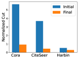
(a)

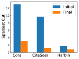
(b)

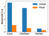
(c)

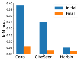
(d)

Figure 2. Results on the initial warm start and the final cut values obtained by NeuroCUT at $k{=}10$. It shows that our neural model NeuroCUT (Final) performs more accurate node and partition selection to optimize the objective function. Subsequently, there is a significant difference between the initial and final cut values.

As detailed in Section 3.2.2, the decoupling of parameter size and the number of partitions allows NeuroCUT to generalize effectively to an unseen number of partitions. In this section, we empirically analyze the generalization performance of NeuroCUT to an unknown number of partitions. We compare it with the non-neural baseline K-means, as the neural methods like GAP, DMon, Ortho, and MinCutPool cannot be employed to infer on an unseen number of partitions. In Table 6, we present the results on inductivity. Specifically, we trained NeuroCUT on different partition sizes ($k=5$ and $k=8$) and tested it on an unseen partition size $k=10$. The inductive version, referred to as NeuroCUT-I, obtains high-quality results on different datasets. Note that while the non-neural method such as K-means needs to be re-run for the unseen partitions, NeuroCUT only needs to perform forward pass to produce the results on an unseen partition size.

4.4. Ablation Studies

Initial Warm Start vs Final Cut Values. NeuroCUT takes a warm start by partitioning nodes based on clustering over their raw node features and Lipschitz embeddings, which are subsequently fine-tuned auto-regressively through the phase 1 and phase 2 of NeuroCUT. In this section, we measure, how much the partitioning objective has improved since the initial clustering? Figure 2 sheds light on this question. Specifically, it shows the difference between the initial cut value after clustering and the final cut value from the partitions produced by our method. We note that there is a significant difference between the initial and final cut values, which essentially shows the effectiveness of NeuroCUT.

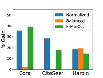
Figure 3. Node Selection in Phase 1 with Heuristic vs Random: Relative % improvement (gain) in cut values obtained by NeuroCUT when using node selection heuristic against random node selection for $k=5$. In most cases, our heuristic finds significantly better cuts than a random node selection procedure.

Impact of Node Selection Procedures. In this section, we explore the effectiveness of our proposed node selection heuristic in enhancing overall quality. Specifically, we measure the relative performance gain(in $\%$) obtained by NeuroCUT when using the node selection heuristic as proposed in Section  3.2.1 over a random node selection strategy. Figure 3 shows the percentage gain for three datasets. We observe that a simpler node selection where we select all the nodes one by one in a random order, yields substantially inferior results in comparison to the heuristic proposed by us. This suggests that the proposed sophisticated node selection strategy plays a crucial role in optimizing the overall performance of NeuroCUT.

5. Conclusion

In this work, we study the problem of graph partitioning with node features. Existing neural methods for addressing this problem require the target objective to be differentiable and necessitate prior knowledge of the number of partitions. In this paper, we introduced NeuroCUT, a framework to effectively address the graph partitioning problem with node features. NeuroCUT tackles these challenges using a reinforcement learning-based approach that can adapt to any target objective function. Further, attributed to its decoupled parameter space and partition count, NeuroCUT can generalize to an unseen number of partitions. The efficacy of our approach is empirically validated through an extensive evaluation on four datasets, four graph partitioning objectives and diverse partition counts. Notably, our method shows significant performance gains when compared to the state-of-the-art techniques, proving its competence in both inductive and transductive settings. In summary, NeuroCUT offers a versatile, inductive, and empirically validated solution for graph partitioning.

Appendix A Appendix

A.1. Additional Related Work

In recent years there has been a growing interest in using machine learning techniques to design heuristics for NP-Hard combinatorial problems on graphs. This line of work is motivated from the observation that traditional algorithmic approaches are limited to using the same heuristic irrespective of the underlying data distribution. Neural approaches, instead, focus on learning the heuristic as a function of the data without deriving explicit algorithms (Duong et al., 2023; Jung and Keuper, 2022; Nazi et al., 2019). Significant advances have been made in learning to solve a variety of combinatorial optimization problems such as Set Cover, Travelling Salesman Problem, Influence Maximization etc. (Khalil et al., 2017; Manchanda et al., 2020; Kool et al., 2018; Joshi et al., 2019). The neural architectural designs in these methods are generally suitable for a specific set of CO problems (Mazyavkina et al., 2021) of similar nature. For instance, AM  (Kool et al., 2018) and NeuroLKH (Xin et al., 2021) are targeted towards routing problems. GCOMB (Manchanda et al., 2020) and LeNSE (Ireland and Montana, 2022) aim to solve problems that are submodular in nature. Owing to these assumptions, the architectural designs in these works are not suitable for our problem of $k$-way inductive graph partitioning with versatile partitioning objectives.

A.2. Clustering for Initialization

As discussed in sec 3.1 in main paper, we first cluster the nodes of the graph into $k$ clusters where $k$ is the number of partitions. Towards this, we apply K-means algorithm (MacQueen et al., 1967) on the nodes of the graph where a node is represented by its raw node features and positional representation i.e $\mathbf{emb_{init}}(u)\;\forall u\in\mathcal{V}$ based upon eq. 8. Further, we used $L_{\inf}$ norm as the distance metric for clustering.

A.3. Dataset Statistics

Table  7 describes the statistics of datasets used in our work. For all datasets we use their largest connected component.

Dataset	$|\mathcal{V}|$	$|\mathcal{E}|$	Number of features
Cora	2485	5069	1433
CiteSeer	2120	3679	3703
Harbin	6598	10492	2
Actor	6198	14879	931

Table 7. Dataset Statistics

A.4. Time complexity of NeuroCUT

We derive the time complexity of forward pass of NeuroCUT as discussed in sec. 3.4 in main paper.

(1) First the positional embeddings for all nodes in the graph are computed. This involves running RWR for $\alpha$ anchor nodes for $\beta$ iterations (Eq.  6). This takes $\mathcal{O}(\alpha\times\beta)$ time. (2) Next, GNN is called to compute embeddings of node. In each layer of GNN a node $v\in\mathcal{V}$ aggregates message from $d$ neighbors where $d$ is the average degree of a node. This takes $\mathcal{O}(\mathcal{V})$ time. This operation is repeat for $L$ layers. Since $L$ is typically 1 or 2 hence we ignore this factor. (3) The node selection algorithm is used that computes score for each node based upon its neighborhood using eq. 10. This consumes $\mathcal{O}(|\mathcal{V}|\times d)$ time. (4) Finally for the selected node, its partition has to be determined using eq. 12 and  13. This takes $\mathcal{O}(d+k)$ time, as we consider only the neighbors of the selected node to compute partition score. Steps 2-4 are repeated for $T^{\prime}$ iterations. Hence overall running time is $\mathcal{O}\big{(}(\alpha\times\beta)+(|\mathcal{V}|\times d+k)\times T^{\prime}\big{)}$. Typically $\alpha$, $\beta$ and $k$ are $<<|\mathcal{V}|$ and $T^{\prime}=o(|\mathcal{V}|)$. Since $|\mathcal{V}|\times d\approx|\mathcal{E}|$, hence complexity is $o(|\mathcal{E}|\times|\mathcal{V}|\big{)}$ Further, for sparse graphs $|\mathcal{E}|=\mathcal{O}(|\mathcal{V}|)$. Hence time complexity of NeuroCUT is $o(|\mathcal{V}|^{2})$.

References

- (1)
- Andersen et al. (2006) Reid Andersen, Fan Chung, and Kevin Lang. 2006. Local graph partitioning using pagerank vectors. In 2006 47th Annual IEEE Symposium on Foundations of Computer Science (FOCS’06). IEEE, 475–486.
- Bianchi et al. (2020) Filippo Maria Bianchi, Daniele Grattarola, and Cesare Alippi. 2020. Spectral clustering with graph neural networks for graph pooling. In International conference on machine learning. PMLR, 874–883.
- Bianchini et al. (2005) Monica Bianchini, Marco Gori, and Franco Scarselli. 2005. Inside pagerank. ACM Transactions on Internet Technology (TOIT) 5, 1 (2005), 92–128.
- Bourgain (1985) Jean Bourgain. 1985. On Lipschitz embedding of finite metric spaces in Hilbert space. Israel Journal of Mathematics 52 (1985), 46–52.
- Chawla et al. (2006) Shuchi Chawla, Robert Krauthgamer, Ravi Kumar, Yuval Rabani, and D Sivakumar. 2006. On the hardness of approximating multicut and sparsest-cut. computational complexity 15 (2006), 94–114.
- Chung (2007) Fan Chung. 2007. Four proofs for the Cheeger inequality and graph partition algorithms. In Proceedings of ICCM, Vol. 2. Citeseer, 378.
- Duong et al. (2023) Chi Thang Duong, Thanh Tam Nguyen, Trung-Dung Hoang, Hongzhi Yin, Matthias Weidlich, and Quoc Viet Hung Nguyen. 2023. Deep MinCut: Learning Node Embeddings by Detecting Communities. Pattern Recognition 134 (2023), 109126.
- Gatti et al. (2022) Alice Gatti, Zhixiong Hu, Tess Smidt, Esmond G Ng, and Pieter Ghysels. 2022. Graph partitioning and sparse matrix ordering using reinforcement learning and graph neural networks. The Journal of Machine Learning Research 23, 1 (2022), 13675–13702.
- Hamilton et al. (2017) Will Hamilton, Zhitao Ying, and Jure Leskovec. 2017. Inductive representation learning on large graphs. Advances in neural information processing systems 30 (2017).
- Ireland and Montana (2022) David Ireland and Giovanni Montana. 2022. Lense: Learning to navigate subgraph embeddings for large-scale combinatorial optimisation. In International Conference on Machine Learning. PMLR, 9622–9638.
- Joshi et al. (2019) Chaitanya K Joshi, Thomas Laurent, and Xavier Bresson. 2019. An efficient graph convolutional network technique for the travelling salesman problem. arXiv preprint arXiv:1906.01227 (2019).
- Jung and Keuper (2022) Steffen Jung and Margret Keuper. 2022. Learning to solve minimum cost multicuts efficiently using edge-weighted graph convolutional neural networks. In Joint European Conference on Machine Learning and Knowledge Discovery in Databases. Springer, 485–501.
- Kahng et al. (2011) Andrew B Kahng, Jens Lienig, Igor L Markov, and Jin Hu. 2011. VLSI physical design: from graph partitioning to timing closure. Vol. 312. Springer.
- Karypis et al. (1997) George Karypis, Rajat Aggarwal, Vipin Kumar, and Shashi Shekhar. 1997. Multilevel hypergraph partitioning: Application in VLSI domain. In Proceedings of the 34th annual Design Automation Conference. 526–529.
- Karypis and Kumar (1998) George Karypis and Vipin Kumar. 1998. Multilevelk-way partitioning scheme for irregular graphs. Journal of Parallel and Distributed computing 48, 1 (1998), 96–129.
- Karypis and Kumar (1999) George Karypis and Vipin Kumar. 1999. Multilevel k-way hypergraph partitioning. In Proceedings of the 36th annual ACM/IEEE design automation conference. 343–348.
- Khalil et al. (2017) Elias Khalil, Hanjun Dai, Yuyu Zhang, Bistra Dilkina, and Le Song. 2017. Learning combinatorial optimization algorithms over graphs. Advances in neural information processing systems 30 (2017).
- Kool et al. (2018) Wouter Kool, Herke Van Hoof, and Max Welling. 2018. Attention, learn to solve routing problems! arXiv preprint arXiv:1803.08475 (2018).
- Li et al. (2005) Hao Li, Gary W Rosenwald, Juhwan Jung, and Chen-Ching Liu. 2005. Strategic power infrastructure defense. Proc. IEEE 93, 5 (2005), 918–933.
- Li et al. (2019) Xiucheng Li, Gao Cong, Aixin Sun, and Yun Cheng. 2019. Learning travel time distributions with deep generative model. In The World Wide Web Conference. 1017–1027.
- MacQueen et al. (1967) James MacQueen et al. 1967. Some methods for classification and analysis of multivariate observations. In Proceedings of the fifth Berkeley symposium on mathematical statistics and probability, Vol. 1. Oakland, CA, USA, 281–297.
- Manchanda et al. (2020) Sahil Manchanda, Akash Mittal, Anuj Dhawan, Sourav Medya, Sayan Ranu, and Ambuj Singh. 2020. Gcomb: Learning budget-constrained combinatorial algorithms over billion-sized graphs. Advances in Neural Information Processing Systems 33 (2020), 20000–20011.
- Mazyavkina et al. (2021) Nina Mazyavkina, Sergey Sviridov, Sergei Ivanov, and Evgeny Burnaev. 2021. Reinforcement learning for combinatorial optimization: A survey. Computers & Operations Research 134 (2021), 105400.
- Nazi et al. (2019) Azade Nazi, Will Hang, Anna Goldie, Sujith Ravi, and Azalia Mirhoseini. 2019. Gap: Generalizable approximate graph partitioning framework. arXiv preprint arXiv:1903.00614 (2019).
- Platonov et al. (2023) Oleg Platonov, Denis Kuznedelev, Michael Diskin, Artem Babenko, and Liudmila Prokhorenkova. 2023. A critical look at the evaluation of GNNs under heterophily: are we really making progress? arXiv preprint arXiv:2302.11640 (2023).
- Pujol et al. (2009) Josep M Pujol, Vijay Erramilli, and Pablo Rodriguez. 2009. Divide and conquer: Partitioning online social networks. arXiv preprint arXiv:0905.4918 (2009).
- Saran and Vazirani (1995) Huzur Saran and Vijay V Vazirani. 1995. Finding k cuts within twice the optimal. SIAM J. Comput. 24, 1 (1995), 101–108.
- Sen et al. (2008) Prithviraj Sen, Galileo Namata, Mustafa Bilgic, Lise Getoor, Brian Galligher, and Tina Eliassi-Rad. 2008. Collective classification in network data. AI magazine 29, 3 (2008), 93–93.
- Shi and Malik (2000) Jianbo Shi and Jitendra Malik. 2000. Normalized cuts and image segmentation. IEEE Transactions on pattern analysis and machine intelligence 22, 8 (2000), 888–905.
- Sutton and Barto (2018) Richard S Sutton and Andrew G Barto. 2018. Reinforcement learning: An introduction. MIT press.
- Tafreshian and Masoud (2020) Amirmahdi Tafreshian and Neda Masoud. 2020. Trip-based graph partitioning in dynamic ridesharing. Transportation Research Part C: Emerging Technologies 114 (2020), 532–553.
- Tsitsulin et al. (2023a) Anton Tsitsulin, John Palowitch, Bryan Perozzi, and Emmanuel Müller. 2023a. Graph clustering with graph neural networks. Journal of Machine Learning Research 24, 127 (2023), 1–21.
- Tsitsulin et al. (2023b) Anton Tsitsulin, John Palowitch, Bryan Perozzi, and Emmanuel Müller. 2023b. Graph clustering with graph neural networks. Journal of Machine Learning Research 24, 127 (2023), 1–21.
- Wang et al. (2017) Chun Wang, Shirui Pan, Guodong Long, Xingquan Zhu, and Jing Jiang. 2017. Mgae: Marginalized graph autoencoder for graph clustering. In Proceedings of the 2017 ACM on Conference on Information and Knowledge Management. 889–898.
- Williams (1992) Ronald J Williams. 1992. Simple statistical gradient-following algorithms for connectionist reinforcement learning. Machine learning 8 (1992), 229–256.
- Xin et al. (2021) Liang Xin, Wen Song, Zhiguang Cao, and Jie Zhang. 2021. NeuroLKH: Combining deep learning model with Lin-Kernighan-Helsgaun heuristic for solving the traveling salesman problem. Advances in Neural Information Processing Systems 34 (2021), 7472–7483.