Finite Time Performance Analysis of MIMO Systems Identification

Abstract

This paper is concerned with the finite time identification performance of an $n$ dimensional discrete-time Multiple-Input Multiple-Output (MIMO) Linear Time-Invariant system, with $p$ inputs and $m$ outputs. We prove that the widely-used Ho-Kalman algorithm and Multivariable Output Error State Space (MOESP) algorithm are ill-conditioned for MIMO system when $n/m$ or $n/p$ is large. Moreover, by analyzing the Cramér–Rao bound, we derive a fundamental limit for identifying the real and stable (or marginally stable) poles of MIMO system and prove that the sample complexity for any unbiased pole estimation algorithm to reach a certain level of accuracy explodes superpolynomially with respect to $n/(pm)$. Numerical results are provided to illustrate the ill-conditionedness of Ho-Kalman algorithm and MOESP algorithm as well as the fundamental limit on identification.

I Introduction

Linear Time-Invariant (LTI) systems are an important class of models with many applications in finance, biology, robotics, and other engineering fields and control applications [1]. Classical results on LTI system identification have mainly focused on guaranteeing asymptotic convergence properties for specific estimation schemes [2], such as ordinary least-squares method (OLS) [3] and subspace identification methods (SIM) [4]. Recently, there has been an increasing interest in finite sample complexity and non-asymptotic analysis [5], and significant progress [6, 7, 8, 9] has been made.

Depending on whether state measurements are directly available, the systems under consideration can be broadly categorized into two classes. For fully observed LTI systems, where the state can be accurately measured, recent works [10, 11, 12, 13] derive upper bounds on identification error of the OLS estimator from a finite number of sample trajectories. However, these error bounds usually depend on the true system parameters, which are unknown during the identification process. Dean et al. [13] further provide a data-dependent upper bound on the identification error. Besides OLS, Wagenmaker and Jamieson  [14] propose an active learning algorithm for identification and derive an error bound. A summary on finite time identification of a fully observed system can be found in [15]. Notice that the above works mainly focus on the upper bound of finite time identification error for specific identification algorithms such as OLS.

On the other hand, Jedra and Proutiere [16] establish lower bounds on sample complexity for a class of locally-stable algorithms in the Probably Approximately Correct (PAC) framework. Tsiamis and Pappas [17] reveal that one can craft a fully observed linear system with non-isotropic noise, where the worst-case sample complexity grows exponentially with the system dimension in the PAC framework, independent of identification algorithm used. However, their result is limited to under-actuated and under-excited linear systems with specific structures.

The identification problem of partially observed LTI systems is considerably more challenging due to the fact that the state cannot be accurately obtained [18]. Some recent works [5, 19, 20, 21] consider a two-step approach to estimate the state-space model from finite input/output sample trajectories: First step, OLS is used to recover Markov parameters from finite input/output data, which in turn allows recovering a balanced state-space realization via the celebrated Ho-Kalman algorithm. As a result, the upper bounds on the finite time identification error of Markov parameters as well as the system matrices can be derived. Another line of research [22, 23, 24] focuses on estimating state-space models using the MOESP algorithm, which is a well-known subspace identification method consisting of estimating the extended observability matrix followed by the system matrices. However, it has been reported in the literature that the subspace method may be ill-conditioned, e.g., see [22, 23]. In addition, other learning-based identification methods, such as reinforcement learning method[25] and gradient descent algorithm [26], have also been proposed to solve the identification problem.

Although bounds on the finite time identification error of specific algorithms, such as Ho-Kalman algorithm or subspace method, have been derived, these bounds usually depend on the true system parameters or input/output trajectories. Hence, it is only possible to prove that the identification problem for a specific system is ill-conditioned. On the other hand, in this paper we provide “uniform” bound of identification error for the Ho-Kalman and MOESP algorithm. As a result, we are able to prove that the two algorithms are ill-conditioned for MIMO system whenever $n/m$ or $n/p$ is large regardless of system parameters, where $n,\,p,\,m$ are the dimensions of the state, input and output respectively. Moreover, we show that the ill-conditionedness is not caused by a specific algorithm design, but fundamentally rooted in the identification problem itself. To this end, we derive a lower bound on the identification error of the stable (or marginally stable) and real poles of MIMO system for any unbiased estimator and further analyze the sample complexity for any unbiased pole estimation algorithm to reach a certain level of accuracy.

The main contribution of this paper is as follows:

1. We prove that the widely-used Ho-Kalman algorithm and MOESP algorithm are ill-conditioned for MIMO system when $n/m$ or $n/p$ is large.

2. We derive a lower bound on the identification error of stable (or marginally stable) and real poles of MIMO system by analyzing the Fisher Information Matrix used in Cramér–Rao bound.

3. We reveal that the sample complexity on the stable (or marginally stable) and real poles of MIMO system using any unbiased estimation algorithm to reach a certain level of accuracy explodes superpolynomially with respect to $n/(pm)$.

Previous versions [27, 28, 29] of this work focus on the identification problem of Single-Input Single-Output (SISO) systems, where in this paper we extend the results to general MIMO system identification.

This paper is organized as follows: Section II formulates the problem and evaluates the finite time performance of the widely-used Ho-Kalman algorithm and MOESP algorithm. Section III derives the Fisher Information matrix of unknown system poles, which is used in Section IV to lower bound the identification error via Cramér–Rao bound and analyze the sample complexity. Section V provides numerical simulations and finally Section VI concludes this paper.

Notations: $\mathbf{0}$ is an all-zero matrix of proper dimensions. For any $x\in\mathbb{R}$, $\lfloor x\rfloor$ denotes the largest integer not exceeding $x$, and $\lceil x\rceil$ denotes the smallest integer not less than $x$. The Frobenius norm is denoted by $\|A\|_{\rm F}=\sqrt{{\rm tr}\left(A^{\rm H}A\right)}$, and $\|A\|$ is the spectral norm of $A$, i.e., its largest singular value $\sigma_{\max}(A)$. $\sigma_{j}(A)$ denotes the $j$-th largest singular value of $A$, and $\sigma_{\min}(A)$ denotes the smallest non-zero singular value of $A$. $\sigma(A)$ denotes the spectrum of a square matrix $A$. The Moore-Penrose inverse of matrix $A$ is denoted by $A^{\dagger}$. ${\rm cond}(A)=\|A\|\|A^{\dagger}\|$ denotes the condition number of $A$. $I_{n}$ denotes the $n\times n$ identity matrix. $\otimes$ is the Kronecker product. The matrix inequality $A\succeq B$ implies that matrix $A-B$ is positive semi-definite. Multivariate Gaussian distribution with mean $\mu$ and covariance $\Sigma$ is denoted by $\mathcal{N}(\mu,\Sigma)$.

II Finite Time Performance Analysis of Classical Identification Algorithms

In this section, we formulate the MIMO system identification problem and evaluate the finite time performance of the widely-used Ho-Kalman algorithm and MOESP algorithm. We consider the identification problem of an observable and controllable LTI system evolving according to

$$x_{k+1} =Ax_{k}+Bu_{k}+w_{k},$$ (1)

$$y_{k} =Cx_{k}+v_{k},$$

based on finite input/output sample data, where $x_{k}\in\mathbb{R}^{n}$, $u_{k}\in\mathbb{R}^{p}$, $y_{k}\in\mathbb{R}^{m}$ are the system state, the input and the output, respectively, and $w_{k}\sim\mathcal{N}(\mathbf{0},\mathcal{Q})$, $v_{k}\sim\mathcal{N}(\mathbf{0},\mathcal{R})$ with $\mathcal{Q},\,\mathcal{R}>0$ are the i.i.d. process and measurement noise respectively and are independent from each other. $A,B,C$ are unknown matrices with appropriate dimensions. For convenience, define

$$\overline{\bm{\delta}}\triangleq\left(\max_{i,j}|b_{ij}|\right)\left(\max_{i,j}|c_{ij}|\right).$$

Assumption 1.

Matrix $A$ is diagonal and its diagonal elements, i.e., the poles of the system (1), are distinct and real. The system is both observable and controllable.

Remark 1.

It is worth noticing that the observability and controllability condition implies that the state-space representation is minimal. Furthermore, since there are infinitely many state-space models similar to system (1), which share the same input-output relationship, Assumption 1 is necessary to make the identification problem well-defined.

It is also worth noticing that Assumption 1 can be extended to include systems containing complex or non-single poles, by focusing on the subsystem consisting of distinct real poles. To be specific, we could use a different realization of (1) with the following form, without changing the input-output relationship of the original system:

$$x_{k+1} =\begin{bmatrix}A_{1}&\\ &A_{2}\end{bmatrix}x_{k}+\begin{bmatrix}B_{1}\\ B_{2}\end{bmatrix}u_{k}+w_{k},$$

$$y_{k} =\begin{bmatrix}C_{1}&C_{2}\end{bmatrix}x_{k}+v_{k},$$

where $A_{1}$ contains the single real poles and $A_{2}$ contains the rest of the poles.

One could assume that the $A_{2},B_{2},C_{2}$ matrices are provided by an oracle, which simplifies the identification problem. However, as will be shown later, even with this additional information, the identification of $A_{1},B_{1},C_{1}$ is still ill-conditioned.

Before continuing on, we shall state several results regarding the (generalized) observability, controllability and the Hankel matrices $O$, $Q$ and $H$ of the system (1), which are defined as:

$$O \triangleq\begin{bmatrix}C^{\top}&(CA)^{\top}&\cdots&(CA^{K_{1}-1})^{\top}\end{bmatrix}^{\top},$$ (2)

$$Q \triangleq\begin{bmatrix}B&AB&\cdots&A^{K_{2}-1}B\end{bmatrix},$$ (3)

$$H \triangleq\begin{bmatrix}CB&CAB&\cdots&CA^{K_{2}-1}B\\ CAB&CA^{2}B&\cdots&CA^{K_{2}}B\\ \vdots&\vdots&\ddots&\vdots\\ CA^{K_{1}-1}B&CA^{K_{1}}B&\cdots&CA^{K_{1}+K_{2}-2}B\end{bmatrix}=OQ,$$ (4)

where $K_{1}$ and $K_{2}$ are large enough such that $O$ and $Q$ are full column and row rank respectively.

The condition number of matrices $O$ and $Q$ and the $n$-th largest singular value of the Hankel matrix $H$ of the system (1) can be characterized by the following Lemma, whose proof is reported in the Appendix:

Lemma 1.

Suppose that the matrices $O$ and $Q$ are full column and row rank respectively, then the condition numbers of $O$ and $Q$ of the system (1) satisfy

$${\rm cond}(O)\geq\frac{1}{4}\rho^{\frac{\lfloor\frac{n-1}{2m}\rfloor}{\log(2mK_{1})}},\quad{\rm cond}(Q)\geq\frac{1}{4}\rho^{\frac{\lfloor\frac{n-1}{2p}\rfloor}{\log(2pK_{2})}},$$ (5)

where $\rho\triangleq e^{\frac{\pi^{2}}{4}}\approx 11.8$.

Moreover, if the system (1) is stable (or marginally stable), then the $n$-th largest singular value of $H$ satisfies the following inequality

$$\sigma_{n}(H)\leq 2\overline{\bm{\delta}}nK\sqrt{pm}\rho^{-\max\left\{\frac{\lfloor\frac{n-1}{2m}\rfloor}{\log(2mK_{1})},\frac{\lfloor\frac{n-1}{2p}\rfloor}{\log(2pK_{2})}\right\}},$$ (6)

where $K=K_{1}+K_{2}$ and $\rho=e^{\pi^{2}/4}$.

In the following two subsections, we shall apply Lemma 1 to analyze the finite time performance of the Ho-Kalman algorithm and MOESP algorithm.

II-A Analysis of Ho-Kalman Algorithm

The Ho-Kalman algorithm [30, 19] is widely used to derive a state-space realization of LTI systems. Before introducing the Ho-Kalman algorithm, first we need to introduce some notations in accordance with [19]. For the system (1), let $\overline{A},\overline{B},\overline{C}$ be the state-space realization corresponding to the output of Ho-Kalman algorithm with true Markov parameter matrices. Let $H^{+}$ and $H^{-}$ are the sub-matrices of $H$ discarding the left-most and right-most $mK_{1}\times p$ block respectively. Denote $L$ as the best rank-$n$ approximation of $H^{-}$.

Step 1: Construct the Hankel matrix $\widehat{H}$ based on Markov parameter matrices estimated from finite input/output sample data.

Step 2: Compute the singular value decomposition (SVD) of the matrix

$$\widehat{L}=\mathcal{U}_{1}\Sigma_{1}\mathcal{V}^{\rm H}_{1},$$

where $\Sigma_{1}$ is a diagonal matrix of the sorted $n$ singular values of $\widehat{L}$, and $\mathcal{U}_{1}$ and $\mathcal{V}_{1}$ are matrices composed of corresponding left and right singular vectors. Indeed, $\mathcal{U}_{1}\Sigma_{1}\mathcal{V}_{1}^{\rm H}$ is the best rank-$n$ approximation (or truncated SVD) of $\widehat{H}^{-}$.

Step 3: Estimate the observability and controllability matrices $O$ and $Q$ from the SVD of matrix $\widehat{L}$:

$${\color[rgb]{0,0,0}\widehat{O}=\mathcal{U}_{1}\Sigma_{1}^{\frac{1}{2}},\quad\widehat{Q}=\Sigma_{1}^{\frac{1}{2}}\mathcal{V}_{1}^{\rm H}.}$$

Step 4: Construct estimates of the state-space matrices as follows

$$\widehat{C}=\widehat{O}(1:m,:),\quad\widehat{B}=\widehat{Q}(:,1:p),\quad\widehat{A}=\widehat{O}^{\dagger}\widehat{H}^{+}\widehat{Q}^{\dagger},$$

where $\widehat{O}(1:m,:)$ is the top-most $m\times n$ block of $\widehat{O}$, and $\widehat{Q}(:,1:p)$ is the left-most $n\times p$ block of $\widehat{Q}$.

For the Ho-Kalman algorithm above, Oymak and Ozay [19] give an upper bound on the identification error in the form of the following theorem, which depends on the true parameters of the system.

Theorem 1 ([19]).

Suppose $\sigma_{n}(H^{-})>0$ and perturbation obeys

$$\|L-\widehat{L}\|\leq\sigma_{n}(H^{-})/2.$$ (7)

Then, there exists a unitary matrix $\mathcal{U}\in\mathbb{R}^{n\times n}$ such that,

$$\|\overline{C}-\widehat{C}\mathcal{U}\|_{\rm F}\leq\|O-\widehat{O}\mathcal{U}\|_{\rm F}\leq{\|L-\widehat{L}\|\sqrt{\frac{10n}{\sigma_{n}(H^{-})}}},$$ (8)

$$\|\overline{B}-\mathcal{U}^{\rm H}\widehat{B}\|_{\rm F}\leq\|Q-\mathcal{U}^{\rm H}\widehat{Q}\|_{\rm F}\leq{\|L-\widehat{L}\|\sqrt{\frac{10n}{\sigma_{n}(H^{-})}}}.$$

Furthermore, hidden state matrices $\widehat{A},\overline{A}$ satisfy

$$\|\overline{A}-\mathcal{U}^{\rm H}\widehat{A}\mathcal{U}\|_{\rm F}\leq\\ {\frac{9\sqrt{n}}{\sigma_{n}(H^{-})}\left(\sqrt{\frac{\|L-\widehat{L}\|}{\sigma_{n}(H^{-})}}\|H^{+}\|+\|H^{+}-\widehat{H}^{+}\|\right).}$$ (9)

According to the above theorem, if the system is stable (or marginally stable), then to ensure a reasonable system identification performance, the error $\|L-\widehat{L}\|$ should be comparable with respect to $\sigma_{n}(H^{-})$.

Using essentially the same argument of Lemma 1, one can show that, if the system (1) is stable (or marginally stable), then the following inequality holds:

$$\sigma_{n}(H_{-})\leq 2\overline{\bm{\delta}}nK\sqrt{pm}\rho^{-\max\left\{\frac{\lfloor\frac{n-1}{2m}\rfloor}{\log(2m(K_{1}-1))},\frac{\lfloor\frac{n-1}{2p}\rfloor}{\log(2pK_{2})}\right\}},$$ (10)

where $K=K_{1}+K_{2}-1$ and $\rho=e^{\pi^{2}/4}\approx 11.8$. As a result, it can be seen that $\sigma(H_{-})$ decays superpolynomially with respect to the largest number between $n/m$ or $n/p$.

On the other hand, if $N$ independent trajectories $(u_{0:K}^{1},y_{0:K}^{1}),\ldots,(u_{0:K}^{N},y_{0:K}^{N})$ are collected, then the convergence of estimated Markov parameters to the true Markov parameters is governed by the central limit theorem. Hence, the variance of $\|L-\widehat{L}\|$ is $O(1/{N})$, which indicates that the number of trajectories required to reach certain accuracy also increase superpolynomially with respect to $n/p$ or $n/m$, whichever is the largest.

II-B Analysis of MOESP Algorithm

In this subsection, we analyze the finite time performance of the widely-used MOESP algorithm [31].

Before introducing the MOESP algorithm, we need to give the definitions of some symbols involved in MOESP algorithm. First, we define the Hankel matrix of past inputs as follows

$$U_{p}\triangleq\begin{bmatrix}u_{0}&\cdots&u_{K_{2}-1}\\ \vdots&\ddots&\vdots\\ u_{K_{1}-1}&\cdots&u_{K_{1}+K_{2}-2}\end{bmatrix}.$$ (11)

We can define the Hankel matrix of past outputs as $Y_{p}$ in the same way. The Hankel matrix of past data is defined by $Z_{p}\triangleq\begin{bmatrix}U_{p}^{\top}&Y_{p}^{\top}\end{bmatrix}^{\top}$.

Here we briefly introduce the MOESP algorithm as follows.

Step 1: Construct matrix $Z_{p}$ based on finite input/output sample data.

Step 2: Perform LQ decomposition to matrix $Z_{p}$, and it can be obtained that

$$\begin{bmatrix}U_{p}\\ Y_{p}\end{bmatrix}=Z_{p}=\begin{bmatrix}L_{11}&\\ L_{21}&L_{22}\end{bmatrix}\begin{bmatrix}Q_{1}^{\top}\\ Q_{2}^{\top}\end{bmatrix},$$ (12)

where $L_{11}$ and $L_{22}$ are $K_{1}\times K_{1}$ matrices.

Step 3: Estimate the observability matrix $O$ from SVD of $L_{22}$:

$$\widehat{O}=\mathcal{U}_{2}\Sigma_{2}^{\frac{1}{2}},$$

where $L_{22}=\mathcal{U}_{2}\Sigma_{2}\mathcal{V}_{2}^{\rm H}$ is SVD of $L_{22}$.

Step 4: Compute estimates of the state-space matrices as follows

$$\widehat{C}=\widehat{O}(1:m,:),\quad\widehat{A}=\underline{\widehat{O}}^{\dagger}\overline{\widehat{O}},$$

where $\underline{\widehat{O}}$ and $\overline{\widehat{O}}$ are the sub-matrices of $\widehat{O}$ discarding the bottom-most and top-most $m\times n$ block respectively. Compute least square estimates of matrix $B$ using equation (23.120) in [33].

Note that the key to MOESP algorithm is to calculate the Moore-Penrose inverse of the observability matrix $O$, which is analogous to Ho-Kalman algorithm. According to Lemma 1, the condition number of $O$ increases at a superpolynomial rate with respect to $n/m$, which means when $n/m$ is large, the identification of matrix $A$ in MOESP algorithm will be ill-conditioned regardless of system parameters.

III Analysis of Fisher Information matrix

In the previous section, we prove that the widely-used Ho-Kalman algorithm and MOESP algorithm are ill-conditioned for MIMO system when $n/m$ or $n/p$ is large. One may wonder if the ill-conditionedness is due to the specific implementation of the Ho-Kalman algorithm and the MOESP algorithm, or is it fundamentally rooted in the identification problem itself. In the following, we prove that the identification problem itself is inherently ill-conditioned in the sense that any unbiased estimator will have an estimation error covariance that grows superpolynomially with respect to $n/(pm)$. To this end, we derive the Fisher Information matrix and further characterize its smallest eigenvalue, which shall be used to lower bound the sample complexity of any unbiased identification algorithm in the next section via Cramér-Rao bound.

III-A Problem Formulation

In order to make the identification problem well-defined, here we consider the following observable and controllable LTI system:

$$x_{k+1} =\underbrace{\begin{bmatrix}\lambda_{1}&\\ &\lambda_{2}&\\ &&\ddots\\ &&&\lambda_{n}\end{bmatrix}}_{A}x_{k}+\underbrace{\begin{bmatrix}b_{11}&\cdots&b_{1p}\\ b_{21}&\cdots&b_{2p}\\ \vdots&\ddots&\vdots\\ b_{n1}&\cdots&b_{np}\\ \end{bmatrix}}_{B}u_{k},$$ (13)

$$y_{k} =\underbrace{\begin{bmatrix}c_{11}&c_{12}&\cdots&c_{1n}\\ \vdots&\vdots&\ddots&\vdots\\ c_{m1}&c_{m2}&\cdots&c_{mn}\\ \end{bmatrix}}_{C}x_{k}+v_{k},$$

which is the diagonal form of the system (1).

Remark 2.

It is worth noticing that there exists infinitely many equivalent state-space models of the system, which are compatible with input and output data and are similar to each other. Hence, To make the identification problem well-conditioned, we choose to identify the diagonal form in this section, since poles play an important role in various controller design methods, e.g., loop-shaping, root locus and so on. We plan to investigate the identifiability of other canonical form, such as the controllability standard form in the future.

It is also worth noticing that we omit the process noise in our formulation. The process noise increases the variance of the measurements. On one hand, this makes the estimation of the mean more difficult. On the other hand, the variance may also contain information regarding the system parameters. Hence, it is still unclear whether the removal of the process noise is helpful or detrimental to the system identification process and we plan to leave it to future investigations.

We further make the following assumptions besides Assumption 1:

Assumption 2.

1. $A$ is unknown, and $B,C$ are known.

2. All eigenvalues of $A$ are stable (or marginally stable), i.e., all eigenvalues of $A$ lie on the line segment $[-1,1]$.

3. For each trajectory, the initial condition of the state $x_{0}=\mathbf{0}$ is known.

4. Without loss of generality, we assume that for each trajectory, the energy of input does not exceed $1$ , i.e, $\sum_{k=0}^{K-1}\|u_{k}^{(\ell)}\|^{2}\leq 1$, where the superscript $\ell$ here represents the label of sample trajectories.

5. Without loss of generality, we assume that measurement noise $v_{k}$ obeys the standard Gaussian, i.e., $\mathcal{R}=I_{m}$.

6. The length $K$ of each trajectory is the same.

Remark 3.

Notice that the assumption that $B,C$ as well as the initial condition $x_{0}=\mathbf{0}$ are known essentially makes the identification problem easier. However, as shall be proved later, even if the identification algorithm has such knowledge, the identification problem is still ill-conditioned when $n/(pm)$ is large.

The main goal of this section is to derive and bound the Fisher Information matrix of unknown poles $\bm{\lambda}$ for MIMO systems, where $\bm{\lambda}\triangleq\begin{bmatrix}\lambda_{1}&\cdots&\lambda_{n}\end{bmatrix}^{\top}$, based on finite number of sample trajectories, i.e., a sequence $\left\{\left(u_{k}^{(\ell)},y_{k+1}^{(\ell)}\right)\right\}_{k=0}^{K-1}$ with $\ell=1,2,\cdots,N$, where $N$ is the number of available sample trajectories and $K$ is the length of each trajectory.

III-B Fisher Information Matrix

In this subsection, we derive the Fisher Information matrix $\mathbf{I}(\bm{\lambda})$ of unknown poles $\bm{\lambda}$ of MIMO systems and further characterize its smallest eigenvalue.

Theorem 2.

For the system (13), under the condition that Assumption 1 and 2 are satisfied, given one sample trajectory with length $K$, the Fisher Information matrix $\mathbf{I}(\bm{\lambda})$ of unknown poles $\bm{\lambda}$ is

$$\mathbf{I}(\bm{\lambda})=V^{\top}S^{\top}SV,$$ (14)

where

$$S=\begin{bmatrix}I_{m}\otimes u_{0}^{\top}&&\\ \vdots&\ddots&\\ I_{m}\otimes u_{K-1}^{\top}&\cdots&I_{m}\otimes u_{0}^{\top}\end{bmatrix}_{mK\times pmK},$$ (15)

and

$$V=\begin{bmatrix}0&\cdots&0\\ \vdots&\ddots&\vdots\\ 0&\cdots&0\\ c_{11}b_{11}&\cdots&c_{1n}b_{n1}\\ \vdots&\ddots&\vdots\\ c_{m1}b_{1p}&\cdots&c_{mn}b_{np}\\ \vdots&\ddots&\vdots\\ (K-1)c_{11}b_{11}\lambda_{1}^{K-2}&\cdots&(K-1)c_{1n}b_{n1}\lambda_{n}^{K-2}\\ \vdots&\ddots&\vdots\\ (K-1)c_{m1}b_{1p}\lambda_{1}^{K-2}&\cdots&(K-1)c_{mn}b_{np}\lambda_{n}^{K-2}\\ \end{bmatrix}_{pmK\times n}.$$ (16)

Corollary 1.

For the system (13), under the condition that Assumption 1 and 2 are satisfied, given $N$ sample trajectories with length $K$, the Fisher Information matrix $\mathbf{I}(\bm{\lambda})$ of unknown poles $\bm{\lambda}$ is

$$\mathbf{I}(\bm{\lambda})=\sum_{\ell=1}^{N}V^{\top}(S^{(\ell)})^{\top}S^{(\ell)}V,$$ (17)

where the superscript $\ell$ of the matrix $S^{(\ell)}$ indicates that it is a matrix formed by the input on the $\ell$-th sample trajectory in the form of (15).

We have the following lemma to bound $(S^{(\ell)})^{\top}S^{(\ell)}$:

Lemma 2.

For each trajectory, if the energy of the input is no more than $1$, then

$$(S^{(\ell)})^{\top}S^{(\ell)}\preceq pmK^{2}I_{pmK}.$$ (18)

Further, if there are $N$ sample trajectories, we have

$$\mathbf{I}(\bm{\lambda})\preceq pmNK^{2}V^{\top}V,$$ (19)

Proof.

According to the definition of $S^{(\ell)}$, we have

$$\|S^{(\ell)}\|\leq\sqrt{mK}\|S^{(\ell)}\|_{\infty}=\sqrt{mK}\sum_{k=0}^{K-1}\|u_{k}^{(\ell)}\|_{1}\leq K\sqrt{pm},$$ (20)

where the second inequality holds because of Cauchy-Schwartz inequality and that the energy of input of each sample trajectory is not more than $1$. Hence,

$$(S^{(\ell)})^{\top}S^{(\ell)}\preceq pmK^{2}I_{pmK},$$ (21)

which completes the proof. ∎

According to Lemma 2, it follows that the smallest eigenvalue of $\mathbf{I}(\bm{\lambda})$ satisfies

$$\lambda_{\min}(\mathbf{I}(\bm{\lambda}))\leq pmNK^{2}\sigma_{\min}^{2}(V).$$ (22)

Thus, to show that $\mathbf{I}(\lambda)$ is ill-conditioned, we only need to focus on $\sigma_{\min}(V)$. For the convenience of notation, we use $\bm{\kappa}$ to denote $\bm{\frac{n}{pm}}$ in the following.

Lemma 3.

Suppose that the matrix $V$ defined in (16) is full column rank, then its smallest singular value satisfies that

$$\sigma_{\min}^{2}(V)\leq 16n^{2}pm\overline{\bm{\delta}}^{2}K^{3}\rho^{-\frac{\lfloor\bm{\kappa}\rfloor-3}{\log(2K)}},$$ (23)

where $\rho=e^{\frac{\pi^{2}}{4}}$.

Further, we can get the following theorem describing the characterization of the smallest eigenvalue of the Fisher Information matrix $\mathbf{I}(\bm{\lambda})$.

Theorem 3.

For the system (13), under the condition that Assumption 1 and 2 are satisfied, based on $N$ sample trajectories with length $K$, suppose that the Fisher Information matrix $\mathbf{I}(\bm{\lambda})$ is full rank, then its smallest eigenvalue satisfies that

$$\lambda_{\min}\left(\mathbf{I}(\bm{\lambda})\right)\leq 16Nn^{2}(pm)^{2}\overline{\bm{\delta}}^{2}K^{5}\rho^{-\frac{\lfloor\bm{\kappa}\rfloor-3}{\log(2K)}},$$ (24)

where $\rho=e^{\frac{\pi^{2}}{4}}$.

Theorem 3 above reveals that for MIMO systems, the smallest eigenvalue of the Fisher information matrix $\lambda_{\min}\left(\mathbf{I}(\bm{\lambda})\right)$ decreases at a superpolynomial rate with respect to $\bm{\kappa}$ ($\bm{\kappa}=\frac{n}{pm}$). In the next section, we shall leverage this result to prove that the system identification problem is ill-conditioned for any unbiased estimator.

IV Analysis of Sample Complexity

In this section, we derive a fundamental limit on identifying unknown poles $\bm{\lambda}$ of MIMO systems via Cramér-Rao bound. Specifically, we prove that any unbiased estimator will have an estimation error covariance that grows superpolynomially with respect to $\bm{\kappa}$, in this sense that the identification problem itself is ill-conditioned. Moreover, we reveal that the sample complexity required to reach a certain level of accuracy for any unbiased pole estimation algorithm explodes superpolynomially with respect to $\bm{\kappa}$.

Theorem 4 ([34]).

[Cramér–Rao bound] It is assumed that the probability density function $f_{\bm{\theta}}(\bm{x})$ satisfies the regularity conditions

$$\mathbb{E}\left[\frac{\partial\log f_{\bm{\theta}}(\bm{x})}{\partial\bm{\theta}}\right]=\mathbf{0},\text{ for all }\bm{\theta},$$

where the expectation is taken with respect to $f_{\bm{\theta}}(\bm{x})$. Then the covariance matrix of any unbiased estimator $\widehat{\bm{\theta}}$ satisfies

$${\rm Cov}[\widehat{\bm{\theta}}]\succeq\mathbf{I}(\bm{\theta})^{-1},$$

where $\mathbf{I}(\bm{\theta})$ is the Fisher Information matrix of $\bm{\theta}$.

Based on Theorem 3 and Theorem 4 above, the following theorem related to the sample complexity can be easily obtained.

Theorem 5.

For the system (13), under the condition that Assumption 1 and 2 are satisfied, based on $N$ sample trajectories with length $K$, suppose that the Fisher Information matrix $\mathbf{I}(\bm{\lambda})$ is full rank, then for any unbiased estimator $\widehat{\bm{\lambda}}$ of unknown system poles $\bm{\lambda}$, the largest eigenvalue of its covariance matrix satisfies

$$\lambda_{\max}\left({\rm Cov}[\widehat{\bm{\lambda}}]\right)\geq\frac{1}{16Nn^{2}(pm)^{2}\overline{\bm{\delta}}^{2}K^{5}}\rho^{\frac{\lfloor\bm{\kappa}\rfloor-3}{\log(2K)}}$$ (25)

$$\sim\Omega\left\{\frac{1}{N\overline{\bm{\delta}}^{2}}\exp\left[\frac{\pi^{2}\bm{\kappa}}{4\log K}-2\log n-2\log(pm)-5\log K\right]\right\},$$

where $\rho=e^{\frac{\pi^{2}}{4}}$.

Now, we analyze the sample complexity for any unbiased pole estimation algorithm, i.e., the number of samples needed to reach a certain level of accuracy. Notice that according to Theorem 5, the largest eigenvalue of the covariance matrix using any unbiased estimator $\widehat{\bm{\lambda}}$ depends on both the number $N$ of sample trajectories and the length $K$ of each trajectory. In the following we shall consider two extreme cases:

1. Consider the case where the identification is conducted using multiple trajectories with the shortest possible length$K=\lceil n/m\rceil+1$. According to Theorem 5, if the largest eigenvalue of the covariance matrix of unbiased estimator $\widehat{\bm{\lambda}}$ of unknown poles is more than a fixed constant $\epsilon>0$, then the number $N$ of sample trajectories must satisfy

   $${\color[rgb]{0,0,1}N\sim\Omega\left\{\frac{\exp\left[\frac{\pi^{2}\bm{\kappa}}{4\log\frac{n}{m}}-7\log n-2\log(pm)+5\log m\right]}{\epsilon\overline{\bm{\delta}}^{2}}\right\}.}$$ (26)

   Note that when $\bm{\kappa}$ is much larger than $pm$, we can further obtain that $N\sim\Omega\left\{\frac{1}{\epsilon\overline{\bm{\delta}}^{2}}\bm{\kappa}^{-16}11.8^{\bm{\kappa}^{1-\varepsilon}}\right\}$, where $\varepsilon>0$ is any small constant. Hence, the number $N$ of trajectories required grows superpolynomially with respect to $\bm{\kappa}$.

2. Consider the case where only a simple trajectory is used. If the largest eigenvalue of the covariance matrix of unbiased estimator $\widehat{\bm{\lambda}}$ of unknown poles is more than a fixed constant $\epsilon>0$, then the length $K$ of the trajectory must satisfy

   $${\color[rgb]{0,0,1}K\sim\Omega\left\{\frac{\exp\left[\left(5\pi^{2}\bm{\kappa}+\log^{2}\left(16\epsilon\overline{\bm{\delta}}^{2}n^{2}(pm)^{2}\right)\right)^{0.5}/10\right]}{\epsilon^{0.1}\overline{\bm{\delta}}^{0.2}n^{0.2}(pm)^{0.2}}\right\}.}$$ (27)

   Note that when $\bm{\kappa}$ is much larger than $pm$ and $16\overline{\bm{\delta}}^{2}n^{2}(pm)^{2}\geq 1/\epsilon$, the term in the brace of (27) can be approximated by $\epsilon^{-0.1}\overline{\bm{\delta}}^{-0.2}\bm{\kappa}^{-0.6}2.02^{\sqrt{\bm{\kappa}}}$. Hence, the length $K$ of the trajectory required also grows superpolynomially with respect to $\bm{\kappa}$.

Remark 4.

Notice that the lower bound on the sample complexity with a single “long” trajectory, albeit still superpolynomial with respect to $\bm{\kappa}$, is significantly smaller than that of multiple “short” trajectories, which suggests that it may be beneficial to use a longer trajectory rather than multiple but shorter trajectories. However, it may be computationally challenging to use a single long trajectory, as both Ho-Kalman and MOESP algorithm requires factorization of matrix whose size is proportional to the length of the trajectory.

Remark 5.

It is worth noticing that the ill-conditionedness of the identification problem is caused by the bad numerical conditions of certain matrices (observability, controllability, Hankel and Fisher information matrix) and the stochastic noise presented in the sensory data. In essence, our results indicate that even very small amount of noise would greatly affect the identification results, and as a consequence, the sample complexity to get a reasonably accurate system model is very high since the noise level needs to be extremely small.

V Numerical Results

In this section, we first consider the identification of a discrete LTI system modeling a heat conduction process [35] in a planar closed region as

$$\frac{\partial\tau}{\partial t}=\alpha\left(\frac{\partial^{2}\tau}{\partial x_{1}^{2}}+\frac{\partial^{2}\tau}{\partial x_{2}^{2}}\right)$$ (28)

with boundary conditions

$$\left.\frac{\partial\tau}{\partial x_{1}}\right|_{t,0,x_{2}}=\left.\frac{\partial\tau}{\partial x_{1}}\right|_{t,l,x_{2}}=\left.\frac{\partial\tau}{\partial x_{2}}\right|_{t,x_{1},0}=\left.\frac{\partial\tau}{\partial x_{2}}\right|_{t,x_{1},l}=0,$$ (29)

where $x_{1}$ and $x_{2}$ represent the coordinates of this planar region, which is a square with slide length $l$, and $\tau(t,x_{1},x_{2})$ denotes the temperature at time $t$ at location $(x_{1},x_{2})$ and the parameter $\alpha$ denotes the thermal conductivity. We use the finite difference method to discretize the PDE into a $4\times 4$ grid with $1$Hz sample frequency.

(a)

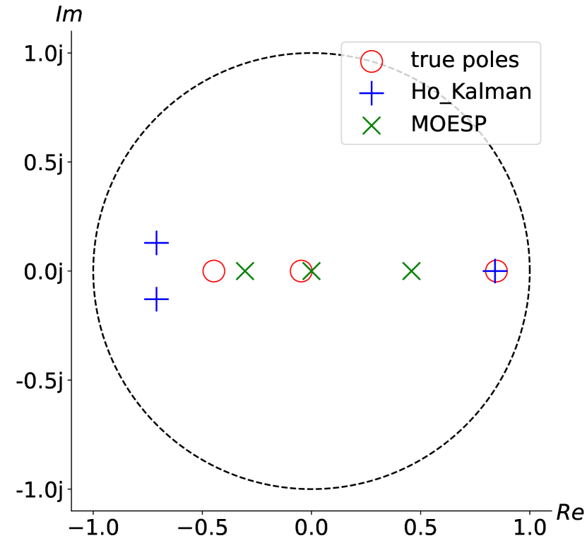
(b)

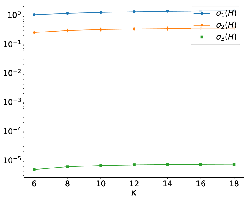
(c)

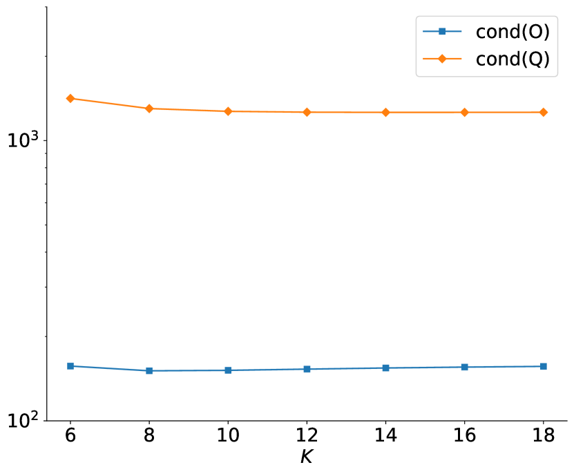
(d)

Figure 1: In sub-figure (a), the red, orange and golden lines correspond to the identification accuracy of the Ho-Kalman algorithm when the number of trajectories $N$ is $10^{2}$, $10^{3}$, and $10^{4}$ respectively, and the blue, green and indigo lines correspond to the identification accuracy of the MOESP algorithm when the number of trajectories $N$ is $10^{2}$, $10^{3}$, and $10^{4}$ respectively. $K$ represents the length of trajectory used for identification. Sub-figure (b) shows the distribution of the true poles (red ‘$\circ$’) and the identified poles (blue ‘$+$’ and green ‘$\times$’ correspond to Ho-Kalman algorithm and MOESP algorithm respectively) in the complex plane when the number of trajectories $N$ is $10^{4}$ and the trajectory length $K$ is $18$, where the dashed line is the unit circle. The blue solid line in sub-figure (c) depicts the smallest singular value of the Hankel matrix $\sigma_{\min}(H)$, and the blue and orange solid line in sub-figure (d) depict the condition numbers of (generalized) observability and controllability matrices $O,Q$.

We further assume that there are $4$ heat sources (sinks) serving as actuators at location $(l/4,l/4)$, $(l/4,3l/4)$, $(3l/4,l/4)$, and $(3l/4,3l/4)$. If we combine the temperature of all grid points at time $k$ into a column vector $T_{k}$, the evolution process of the discrete LTI system can be expressed as

$$T_{k+1}=AT_{k}+Bu_{k}+w_{k},$$ (30)

where $w_{k}\sim\mathcal{N}(\mathbf{0},\mathcal{Q})$ denotes the i.i.d. process noise at time $k$. We assume there is a sensor deployed in the center $(l/2,l/2)$ of the grid, and it measures a linear combination of temperature at grid points around it. Therefore,the measurement $y_{k}$ can be expressed as

$$y_{k}=CT_{k}+v_{k},$$ (31)

where $v_{k}\sim\mathcal{N}(0,\mathcal{R})$ denotes the i.i.d. measurement noise. For numerical experiments, we set the parameters to the following values:

• $\alpha=0.2$; $l=3$;

• $\mathcal{Q}=I_{16}$, $\mathcal{R}=1$; $u_{k}\sim\mathcal{N}(0,1)$.

Since the system matrix $A$ contains double root and the system is neither controllable nor observable, a Kalman decomposition is performed to reduce the model into its minimal controllable and observable realization $(A_{r},B_{r},C_{r})$, which contains $3$ internal states.

Ho-Kalman algorithm and MOESP algorithm are used to identify the system matrix of the minimal realization from multiple independent trajectories collected. The result obtained is depicted in Fig 1. We use the Hausdorff distance to measure the distance between the true and the identified spectrum, which is defined as

$$d_{\rm Hausdorff}(A_{r},\widehat{A}_{r})\triangleq\max\{\max_{i}\min_{j}|\lambda_{i}-\hat{\lambda}_{j}|,\max_{j}\min_{i}|\lambda_{i}-\hat{\lambda}_{j}|\},$$

where $\lambda_{i}$s and $\hat{\lambda}_{i}$s are the eigenvalues of $A_{r}$ and $\widehat{A}_{r}$ matrices respectively. It can be seen that the Hausdorff distances for both algorithms are all greater than $0.3$, and does not improve much even with more trajectories collected. Notice that for the minimal system, all the $3$ poles are real due to the symmetry of the $A$ matrix and the spectral radius is $0.85$. Hence, a trivial guess of $\widehat{A}_{r}=\mathbf{0}$ would provide a Hausdorff distance no more than $0.85$, which implies that even with $10^{4}$ trajectories collected, the Ho-Kalman algorithm and MOESP algorithm are not doing better than a trivial guess. On the other hand, it can be seen that $\sigma_{\min}(H)$ is minuscule and the condition numbers of (generalized) observability and controllability matrices $O,Q$ are gargantuan, which shows that both identification algorithms are ill-conditioned.

Next, we give numerical results of the $n$-th largest singular value of the Hankel matrix $H$, the condition number of the observability matrix $O$ in Ho-Kalman algorithm and MOESP algorithm, and our bounds derived in Theorem 1 in Fig. 4 and 4. In the numerical experiments about matrices $H$ and $O$, we set the number $p$ of inputs to 1, and the number $m$ of outputs to 1, and $K_{1}$ to $\lceil n/m\rceil=n$, and $K_{2}$ to $\lceil n/p\rceil=n$, and $A$ to be a diagonal matrix where its diagonal elements and all elements of matrices $B$, $C$ are uniformly sampled from the line segment $[-1,1]$. For each $n$, we repeat $10^{4}$ trials.

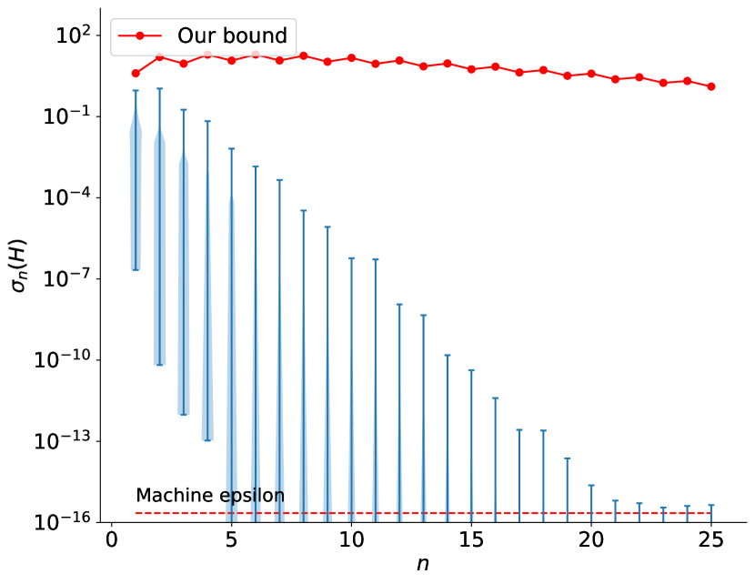
Figure 2: Numerical results of the key matrix $H$ in Ho-Kalman algorithm. The blue violinplot represents the sampling distribution of the $n$-th largest singular value of the Hankel matrix $H$ in different dimension $n$. The red dashed and solid lines represent machine epsilon and the bound we derive in (6), respectively.

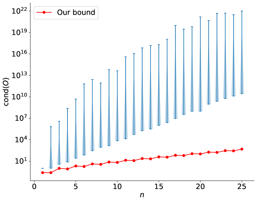
Figure 3: Numerical results of the key matrix $O$ in Ho-Kalman/MOESP algorithm. The blue violinplot represents the sampling distribution of the condition number of the observability matrix $O$ in different dimension $n$. The red solid line represents the bound we derive in (5).

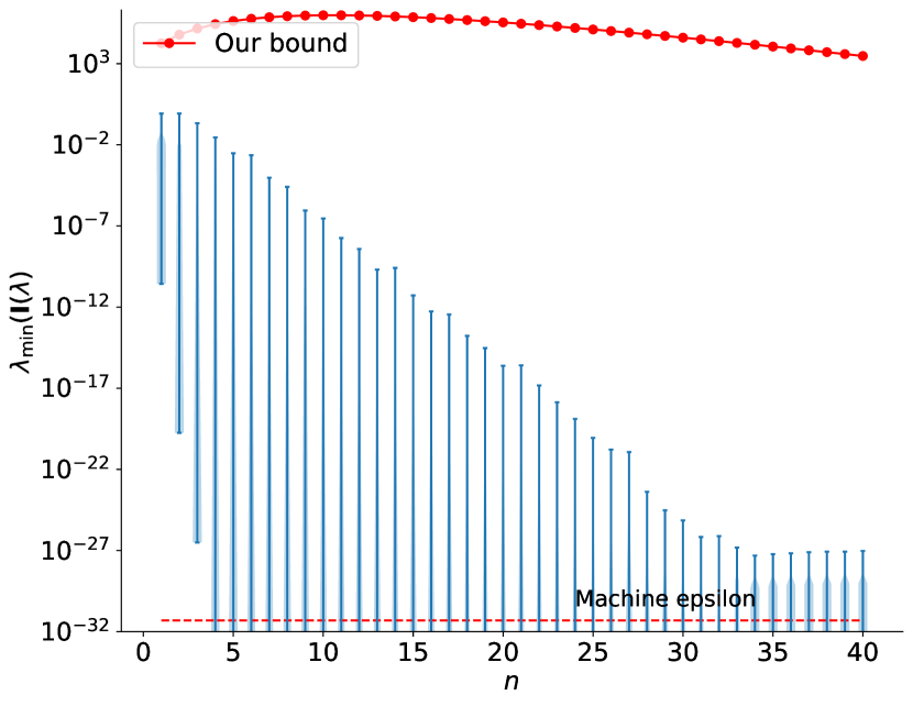
Figure 4: Numerical results of Fisher Information matrix $\mathbf{I}(\bm{\lambda})$. The blue violinplot represents the sampling distribution of the smallest eigenvalue of Fisher Information matrix $\mathbf{I}(\bm{\lambda})$ in different dimension $n$. The red dashed and solid lines represent machine epsilon and the bound we derive in (24), respectively.

Finally, the numerical results of the smallest eigenvalue of the Fisher Information matrix $\mathbf{I}(\bm{\lambda})$ of unknown poles and our upper bound derived in Theorem 3 are depicted in Fig. 4. In the numerical experiments about Fisher Information matrix, we set the measurement noise $v_{k}$ to obey the standard Gaussian, the number $N$ of trajectories to 1, the energy of the input to $1$, the number $p$ of inputs to 1, and the number $m$ of outputs to 1, and the length $K$ of the trajectory to $n+1$. Also, the diagonal elements of matrix $A$ and all elements of matrices $B,C$ are uniformly sampled from the line segment $[-1,1]$. For each $n$, we repeat $10^{4}$ trials.

It can be seen that our bounds are valid, However, the sampled system is much more ill-conditioned than our results suggested. Since our “uniform” bound works for any system, there may exist some $A,\,B,\,C$ matrices which make the identification problem “less” ill-conditioned, but is not sampled due to the limited sample size. On the other hand, we think that there may be ways to strengthen our bounds, which we plan to investigate in the future.

VI Conclusion

This paper considers the finite time identification performance of an $n$ dimensional discrete-time MIMO LTI system, with $p$ inputs and $m$ outputs. We first prove that the widely-used Ho-Kalman algorithm and MOESP algorithm are ill-conditioned for MIMO systems when $n/m$ or $n/p$ is large. Moreover, a fundamental limit on MIMO system identification is derived by analyzing the Fisher Information Matrix used in Cramér–Rao bound. Based on this analysis, we reveal that the sample complexity on unknown poles of stable (or marginally stable) MIMO systems using any unbiased estimation algorithm to a certain level of accuracy explodes superpolynomially with respect to $n/(pm)$. Future works include tightening our bound while designing system identification algorithms that can approach the fundamental limit.

VII Appendix

VII-A Preliminaries

Lemma 4.

Given a $n\times mp$ ($p\leq n$) matrix $X_{n,mp}$ satisfying

$$X_{n,mp}=\begin{bmatrix}W_{p}&DW_{p}&\cdots&D^{m-1}W_{p}\end{bmatrix},$$ (32)

where $W_{p}\in\mathbb{R}^{n\times p}$ and $D$ is a unitary diagonalizable matrix with real eigenvalues, then the smallest singular value of $X_{n,mp}$ satisfies

$$\sigma_{\min}(X_{n,mp})\leq 4\rho^{-\frac{\lfloor\frac{\min\{n,m(p-[p]_{*})\}-1}{2p}\rfloor}{\log(2mp)}}\|X_{n,mp}\|,$$

where $\rho\triangleq e^{\frac{\pi^{2}}{4}}$, and $[p]_{*}=0$ if $p$ is even or $p=1$ and is $1$ if $p$ is an odd number greater than $1$.

Proof.

If $p$ is equal to $1$, the proof can be directly completed based on Corollary 5.3 in [36], thus in the following we consider the case where $p$ is greater than $1$. It is not difficult to verify that matrix $X_{n,mp}$ satisfies the following Sylvester matrix equation:

$$DX_{n,mp}-X_{n,mp}P=\begin{bmatrix}\mathbf{0}_{n\times(m-1)p}&D^{m}W_{p}-W_{p}D_{1}\end{bmatrix},$$ (33)

where $P=\begin{bmatrix}&D_{1}\\ I_{(m-1)p}&\end{bmatrix}$, and $D_{1}=\begin{bmatrix}1&\\ &-I_{p-1}\end{bmatrix}$.

The following analysis is somewhat similar to the content of Section 5.1 in [36]. For completeness, here we give a complete proof. For the following analysis, it can be assumed that $p$ is even. This is without loss of generality, since we can use Cauchy interlace theorem [37]. To see this, if $p$ is an odd number greater than $1$, let matrix $W_{p-1}$ be the $n\times(p-1)$ matrix obtained from $W_{p}$ by removing its last column and $X_{n,m(p-1)}$ be

$$\begin{bmatrix}W_{p-1}&DW_{p-1}&\cdots&D^{m-1}W_{p-1}\end{bmatrix}.$$

According to Cauchy interlace theorem [37], it can be obtained that

$$\sigma_{\min}(X_{n,mp})\leq\sigma_{\min}(X_{n,m(p-1)})\leq\|X_{n,m(p-1)}\|\leq\|X_{n,mp}\|,$$

this implies that

$$\frac{\sigma_{\min}(X_{n,mp})}{\|X_{n,mp}\|}\leq\frac{\sigma_{\min}(X_{n,m(p-1)})}{\|X_{n,m(p-1)}\|}.$$ (34)

In the following, we assume that $p$ is even. Note that matrices $D$ and $P$ in Sylvester matrix equation (33) are both normal matrices. The eigenvalues of $D$ are real numbers, and the eigenvalues of $P$ are the $mp$ (shifted) roots of unity, i.e,

$$\sigma(P)=\left\{z\in\mathbb{C}|z^{mp}=-1\right\}.$$

Since $p$ is even, the spectrum $\sigma(P)$ of $P$ does not intersect the real axis. On the other hand, the rank of $D^{m}W_{p}-W_{p}D_{1}$ does not exceed $p$. Applying Theorem 2.1, Corollary 3.2 and Lemma 5.1 in [36] yields that

$$\sigma_{\min}(X_{n,mp})\leq 4\rho^{-\frac{\lfloor\frac{\min\{n,mp\}-1}{2p}\rfloor}{\log(2mp)}}\|X_{n,mp}\|.$$ (35)

If $p$ is odd, then the proof can be completed according to (34) and (35). ∎

Lemma 5 ([36]).

Let $H_{n}$ be an $n\times n$ real positive definite Hankel matrix, then

$$\sigma_{j+2k}(H_{n})\leq 16\rho^{-\frac{2k-2}{\log(2n)}}\sigma_{j}(H_{n}),1\leq j+2k\leq n,$$ (36)

where $\rho=e^{\frac{\pi^{2}}{4}}$.

Proof.

This is a direct corollary of Corollary 5.5 in the reference [36]. ∎

VII-B Proof of Lemma 1

Proof.

Note that to make $O$, $Q$ full column and row rank respectively, the following inequalities must hold:

$$n\leq mK_{1},\,n\leq pK_{2}.$$

Since $O,\,Q$ are order-$n$ matrices, applying Lemma 4 gives that

$$\sigma_{n}(O)\leq 4\rho^{-\frac{\lfloor\frac{n-1}{2m}\rfloor}{\log(2mK_{1})}}\|O\|\leq 4\rho^{-\frac{\lfloor\frac{n-1}{2m}\rfloor}{\log(2mK_{1})}}\|O\|_{\rm F}$$ (37)

and

$$\sigma_{n}(Q)\leq 4\rho^{-\frac{\lfloor\frac{n-1}{2p}\rfloor}{\log(2pK_{2})}}\|Q\|\leq 4\rho^{-\frac{\lfloor\frac{n-1}{2p}\rfloor}{\log(2pK_{2})}}\|Q\|_{\rm F}.$$ (38)

Then (5) is a direct corollary of (37) and (38).

On the other hand, since $H=OQ$, it is not difficult to get that

$$\sigma_{n}(H)\leq\min\left\{\|Q\|\sigma_{n}(O),\|O\|\sigma_{n}(Q)\right\}$$ (39)

by using the properties of singular values. It can be easily verified that

$$\|O\|_{\rm F}^{2}=\sum_{k=0}^{K_{1}-1}\|CA^{k}\|_{\rm F}^{2}\leq\sum_{k=0}^{K_{1}-1}\|C\|_{\rm F}^{2}\|A^{k}\|^{2}\leq\overline{c}^{2}mnK_{1},$$ (40)

where $\overline{c}=\max_{i,j}|c_{ij}|$, and

$$\|Q\|_{\rm F}^{2}=\sum_{k=0}^{K_{2}-1}\|A^{k}B\|_{\rm F}^{2}\leq\sum_{k=0}^{K_{2}-1}\|B\|_{\rm F}^{2}\|A^{k}\|^{2}\leq\overline{b}^{2}pnK_{2},$$ (41)

where $\overline{b}=\max_{i,j}|b_{ij}|$. Combining the above results and this fact that $K_{1}+K_{2}=K$, we can complete the proof of (6). ∎

VII-C Proof of Lemma 3

Proof.

Consider the following matrix $\widetilde{V}$

$$\widetilde{V}=\begin{bmatrix}\widetilde{V}_{11}^{\top}&\widetilde{V}_{12}^{\top}&\cdots&\widetilde{V}_{mp}^{\top}\end{bmatrix}^{\top}_{pm(K-1)\times n},$$ (42)

where for any $1\leq i\leq m$, $1\leq j\leq p$,

$$\widetilde{V}_{ij} =\begin{bmatrix}c_{i1}b_{1j}&\cdots&c_{in}b_{nj}\\ 2c_{i1}b_{1j}\lambda_{1}&\cdots&2c_{in}b_{nj}\lambda_{n}\\ \vdots&\ddots&\vdots\\ (K-1)c_{i1}b_{1j}\lambda_{1}^{K-2}&\cdots&(K-1)c_{in}b_{nj}\lambda_{n}^{K-2}\\ \end{bmatrix}$$ (43)

$$=\underbrace{\begin{bmatrix}1&\\ &2&\\ &&\ddots&\\ &&&K-1\end{bmatrix}}_{\Lambda_{K-1}}\underbrace{\begin{bmatrix}1&1&\cdots&1\\ \lambda_{1}&\lambda_{2}&\cdots&\lambda_{n}\\ \vdots&\vdots&\ddots&\vdots\\ \lambda_{1}^{K-2}&\lambda_{2}^{K-2}&\cdots&\lambda_{n}^{K-2}\end{bmatrix}}_{\mathbf{V}_{K-1}}$$

$$\qquad\qquad\underbrace{\begin{bmatrix}c_{i1}b_{1j}&\\ &c_{i2}b_{2j}&\\ &&\ddots&\\ &&&c_{in}b_{nj}\end{bmatrix}}_{\Lambda_{ij}}.$$

It can be easily verified that $V$ and $\widetilde{V}$ have the same non-zero singular values, thus we only need to analyze the matrix $\widetilde{V}$. Note that $\widetilde{V}$ can be rewritten as

$$\widetilde{V}=\left(I_{pm}\otimes\Lambda_{K-1}\right)\left(I_{pm}\otimes\mathbf{V}_{K-1}\right)\underbrace{\begin{bmatrix}\Lambda_{11}\\ \Lambda_{12}\\ \vdots\\ \Lambda_{pm}\end{bmatrix}}_{\Lambda}.$$ (44)

Note that to make the matrix $V$ full rank, there must be that $K\geq\lceil\bm{\kappa}\rceil+1$, where $\bm{\kappa}=n/(pm)$, then it follows that

$$\sigma_{\min}^{2}(V)=\sigma_{\min}^{2}(\widetilde{V})\leq K^{2}\|\Lambda\|^{2}\lambda_{\lfloor\bm{\kappa}\rfloor}(\mathbf{V}_{K-1}\mathbf{V}_{K-1}^{\top}).$$ (45)

Note that $\|\Lambda\|^{2}\leq\|\Lambda\|_{\rm F}^{2}\leq npm\overline{\bm{\delta}}^{2}$, thus next we only analyze $\lambda_{\lfloor\bm{\kappa}\rfloor}(\mathbf{V}_{K-1}\mathbf{V}_{K-1}^{\top})$. Using Lemma 5 above yields that

$$\lambda_{\lfloor\bm{\kappa}\rfloor}(\mathbf{V}_{K-1}\mathbf{V}_{K-1}^{\top})\leq 16\rho^{-\frac{\lfloor\bm{\kappa}\rfloor-3}{\log(2K)}}\|\mathbf{V}_{K-1}\mathbf{V}_{K-1}^{\top}\|.$$ (46)

Note that $\|\mathbf{V}_{K-1}\mathbf{V}_{K-1}^{\top}\|\leq\|\mathbf{V}_{K-1}\|_{\rm F}^{2}\leq nK$, then combining it with the above results can complete the proof. ∎

VII-D Proof of Theorem 2

Proof.

The dynamic response of the system (13) in the first $K$ time steps is as follow

$$\underbrace{\begin{bmatrix}y_{1}\\ y_{2}\\ \vdots\\ y_{K}\end{bmatrix}}_{Y_{[1,K]}}=\underbrace{\begin{bmatrix}H_{0}&&&\\ H_{1}&H_{0}&&\\ \vdots&\vdots&\ddots&\\ H_{K-1}&H_{K-2}&\cdots&H_{0}\end{bmatrix}}_{\mathcal{H}_{k}}\underbrace{\begin{bmatrix}u_{0}\\ u_{1}\\ \vdots\\ u_{K-1}\end{bmatrix}}_{U_{[0,K-1]}}+\underbrace{\begin{bmatrix}v_{1}\\ v_{2}\\ \vdots\\ v_{K}\end{bmatrix}}_{V_{[1,K]}},$$

where $H_{k}=CA^{k}B$ is the $k$-th Markov parameter of the system (13).

Since the measurement noise $V_{[1,K]}$ is Gaussian, and the input $U_{[0,K-1]}$ is known, the output $Y_{[1,K]}$ is also Gaussian and its probability density function conditioned on the value of system poles $\bm{\lambda}$ can be obtained as

$$f_{\bm{\lambda}}\left(Y_{[1,K]}\right)=\frac{\exp\left(-\frac{1}{2}\left(Y_{[1,K]}-\mu_{K}\right)^{\top}\left(Y_{[1,K]}-\mu_{K}\right)\right)}{\sqrt{(2\pi)^{K}}},$$ (47)

where $\mu_{K}\triangleq\mathcal{H}_{K}U_{[0,K-1]}$ represents the mean of $Y_{[1,K]}$. According to the definition of Fisher Information matrix, the $(i,j)$ element of the Fisher Information matrix $\mathbf{I}\left(\bm{\lambda}\right)$ of unknown poles $\bm{\lambda}$ has the following form

$$\mathbf{I}_{i,j}\left(\bm{\lambda}\right)=\mathbb{E}\left[\frac{\partial}{\partial\lambda_{i}}\log f_{\bm{\lambda}}\left(Y_{[1,K]}\right)\frac{\partial}{\partial\lambda_{j}}\log f_{\bm{\lambda}}\left(Y_{[1,K]}\right)\right],$$

where the notation $\mathbb{E}$ is the expectation operator with respect to $f_{\bm{\lambda}}\left(Y_{[1,K]}\right)$. Since the output $Y_{[1,K]}$ is Gaussian, based on the results of section 3.9 of [34], we can further get that

$$\mathbf{I}_{i,j}\left(\bm{\lambda}\right) =\left[\frac{\partial\mu_{K}}{\partial\lambda_{i}}\right]^{\top}\frac{\partial\mu_{K}}{\partial\lambda_{j}},$$ (48)

where $\frac{\partial\mu_{K}}{\partial\lambda_{i}}=\begin{bmatrix}\frac{\partial[\mu_{K}]_{1}}{\partial\lambda_{i}}&\frac{\partial[\mu_{K}]_{2}}{\partial\lambda_{i}}&\cdots&\frac{\partial[\mu_{K}]_{mK}}{\partial\lambda_{i}}\end{bmatrix}^{\top}$, and $[\mu_{K}]_{j}$ denotes the $j$-th entry of $\mu_{K}$ for each $j=1,2,\cdots,mK$. Based on (48), the Fisher Information matrix $\mathbf{I}(\bm{\lambda})$ can be obtained as follow

$$\mathbf{I}\left(\bm{\lambda}\right)=\underbrace{\begin{bmatrix}\frac{\partial\mu_{K}}{\partial\lambda_{1}}&\cdots&\frac{\partial\mu_{K}}{\partial\lambda_{n}}\end{bmatrix}^{\top}}_{\mathcal{L}_{\bm{\lambda}}^{\top}}\underbrace{\begin{bmatrix}\frac{\partial\mu_{K}}{\partial\lambda_{1}}&\cdots&\frac{\partial\mu_{K}}{\partial\lambda_{n}}\end{bmatrix}}_{\mathcal{L}_{\bm{\lambda}}}.$$ (49)

According to the chain derivation rule, $\mathcal{L}_{\bm{\lambda}}$ can be decomposed as follow

$$\mathcal{L}_{\bm{\lambda}}=\begin{bmatrix}\frac{\partial\mu_{K}}{\partial\lambda_{1}}&\cdots&\frac{\partial\mu_{K}}{\partial\lambda_{n}}\end{bmatrix}=\\ \underbrace{\begin{bmatrix}\frac{\partial\mu_{K}}{\partial[H_{0}]_{11}}&\cdots&\frac{\partial\mu_{K}}{\partial[H_{K-1}]_{pm}}\end{bmatrix}}_{S}\underbrace{\begin{bmatrix}\frac{\partial[H_{0}]_{11}}{\partial\lambda_{1}}&\cdots&\frac{\partial[H_{0}]_{11}}{\partial\lambda_{n}}\\ \frac{\partial[H_{0}]_{12}}{\partial\lambda_{1}}&\cdots&\frac{\partial[H_{0}]_{12}}{\partial\lambda_{n}}\\ \vdots&\ddots&\vdots\\ \frac{\partial[H_{K-1}]_{pm}}{\partial\lambda_{1}}&\cdots&\frac{\partial[H_{K-1}]_{pm}}{\partial\lambda_{n}}\end{bmatrix}}_{V}.$$ (50)

Combined with the expressions of $\mu_{K}$ and $H_{k}$, it is not difficult to get the expressions of $S$ and $V$ as shown in (15) and (16), respectively. ∎

VII-E Proof of Theorem 5

Proof.

According to Theorem 3, Theorem 4 and the proof of Theorem 2, we only need to verify that the probability density function $f_{\bm{\lambda}}\left(Y_{[1,K]}\right)$ in (47) satisfies the regularity conditions

$$\mathbb{E}\left[\frac{\partial\log f_{\bm{\lambda}}\left(Y_{[1,K]}\right)}{\partial\lambda_{i}}\right]=0,\text{ for each }i=1,2,\cdots,n,$$

where the expectation is taken with respect to $f_{\bm{\lambda}}\left(Y_{[1,K]}\right)$. For each $i=1,2,\cdots,n$, it follows that

$$\frac{\partial\log f_{\bm{\lambda}}\left(Y_{[1,K]}\right)}{\partial\lambda_{i}} =-\frac{1}{2}\frac{\partial}{\partial\lambda_{i}}\left(Y_{[1,K]}-\mu_{K}\right)^{\top}\left(Y_{[1,K]}-\mu_{K}\right)$$ (51)

$$=\sum_{j=1}^{mK}\left(\left[Y_{[1,K]}\right]_{j}-\left[\mu_{K}\right]_{j}\right)\frac{\partial}{\partial\lambda_{i}}\left[\mu_{K}\right]_{j},$$

where $\left[Y_{[1,K]}\right]_{j}$ and $[\mu_{K}]_{j}$ denote the $j$-th entry of $\mu_{K}$ and $Y_{[1,K]}$, respectively. Now take the expectation of both sides with respect to $f_{\bm{\lambda}}\left(Y_{[1,K]}\right)$, then we can get that

$$\mathbb{E}\left[\frac{\partial\log f_{\bm{\lambda}}\left(Y_{[1,K]}\right)}{\partial\lambda_{i}}\right] =\mathbb{E}\left[\sum_{j=1}^{mK}\left(\left[Y_{[1,K]}\right]_{j}-\left[\mu_{K}\right]_{j}\right)\frac{\partial}{\partial\lambda_{i}}\left[\mu_{K}\right]_{j}\right]$$ (52)

$$=\sum_{j=1}^{mK}\mathbb{E}\left[\left[Y_{[1,K]}\right]_{j}-\left[\mu_{K}\right]_{j}\right]\frac{\partial}{\partial\lambda_{i}}\left[\mu_{K}\right]_{j}$$

$$=0,$$

where the last equality holds because $Y_{[1,K]}$ is Gaussian with mean $\mu_{K}$, which completes the proof. ∎

References

- [1] Lennart Ljung. System identification: theory for the user prentice-hall, inc. Upper Saddle River, NJ, USA, 1986.
- [2] Graham C. Goodwin and Robert L. Payne. DYNAMIC SYSTEM IDENTIFICATION. Elsevier, 1977.
- [3] Lennart Ljung. Consistency of the least-squares identification method. IEEE Transactions on Automatic Control, 21(5):779–781, 1976.
- [4] Manfred Deistler, K Peternell, and Wolfgang Scherrer. Consistency and relative efficiency of subspace methods. Automatica, 31(12):1865–1875, 1995.
- [5] Yang Zheng and Na Li. Non-asymptotic identification of linear dynamical systems using multiple trajectories. IEEE Control Systems Letters, 5(5):1693–1698, 2020.
- [6] Marco C Campi and Erik Weyer. Finite sample properties of system identification methods. IEEE Transactions on Automatic Control, 47(8):1329–1334, 2002.
- [7] M Vidyasagar and Rajeeva L Karandikar. A learning theory approach to system identification and stochastic adaptive control. Journal of Process Control, 18:421–430, 2008.
- [8] Algo Care, Balázs Cs Csáji, Marco C Campi, and Erik Weyer. Finite-sample system identification: An overview and a new correlation method. IEEE Control Systems Letters, 2(1):61–66, 2017.
- [9] Salar Fattahi, Nikolai Matni, and Somayeh Sojoudi. Learning sparse dynamical systems from a single sample trajectory. In 2019 IEEE 58th Conference on Decision and Control (CDC), pages 2682–2689. IEEE, 2019.
- [10] Max Simchowitz, Horia Mania, Stephen Tu, Michael I Jordan, and Benjamin Recht. Learning without mixing: Towards a sharp analysis of linear system identification. In Conference On Learning Theory, pages 439–473. PMLR, 2018.
- [11] Mohamad Kazem Shirani Faradonbeh, Ambuj Tewari, and George Michailidis. Finite time identification in unstable linear systems. Automatica, 96:342–353, 2018.
- [12] Tuhin Sarkar and Alexander Rakhlin. Near optimal finite time identification of arbitrary linear dynamical systems. In International Conference on Machine Learning, pages 5610–5618. PMLR, 2019.
- [13] Sarah Dean, Horia Mania, Nikolai Matni, Benjamin Recht, and Stephen Tu. On the sample complexity of the linear quadratic regulator. Foundations of Computational Mathematics, 20(4):633–679, 2020.
- [14] Andrew Wagenmaker and Kevin Jamieson. Active learning for identification of linear dynamical systems. In Conference on Learning Theory, pages 3487–3582. PMLR, 2020.
- [15] Nikolai Matni and Stephen Tu. A tutorial on concentration bounds for system identification. In 2019 IEEE 58th Conference on Decision and Control (CDC), pages 3741–3749. IEEE, 2019.
- [16] Yassir Jedra and Alexandre Proutiere. Sample complexity lower bounds for linear system identification. In 2019 IEEE 58th Conference on Decision and Control (CDC), pages 2676–2681. IEEE, 2019.
- [17] Anastasios Tsiamis and George J Pappas. Linear systems can be hard to learn. In 2021 60th IEEE Conference on Decision and Control (CDC), pages 2903–2910. IEEE, 2021.
- [18] Yang Zheng, Luca Furieri, Maryam Kamgarpour, and Na Li. Sample complexity of linear quadratic gaussian (lqg) control for output feedback systems. In Learning for Dynamics and Control, pages 559–570. PMLR, 2021.
- [19] Samet Oymak and Necmiye Ozay. Revisiting ho–kalman-based system identification: Robustness and finite-sample analysis. IEEE Transactions on Automatic Control, 67(4):1914–1928, 2021.
- [20] Max Simchowitz, Ross Boczar, and Benjamin Recht. Learning linear dynamical systems with semi-parametric least squares. In Conference on Learning Theory, pages 2714–2802. PMLR, 2019.
- [21] Anastasios Tsiamis and George J Pappas. Finite sample analysis of stochastic system identification. In 2019 IEEE 58th Conference on Decision and Control (CDC), pages 3648–3654. IEEE, 2019.
- [22] Alessandro Chiuso and Giorgio Picci. On the ill-conditioning of subspace identification with inputs. Automatica, 40(4):575–589, 2004.
- [23] Slim Hachicha, Maher Kharrat, and Abdessattar Chaari. N4sid and moesp algorithms to highlight the ill-conditioning into subspace identification. International Journal of Automation and Computing, 11(1):30–38, 2014.
- [24] Kenji Ikeda and Hiroshi Oku. Estimation error analysis of system matrices in some subspace identification methods. In 2015 10th Asian Control Conference (ASCC), pages 1–6. IEEE, 2015.
- [25] Sahin Lale, Kamyar Azizzadenesheli, Babak Hassibi, and Anima Anandkumar. Logarithmic regret bound in partially observable linear dynamical systems. Advances in Neural Information Processing Systems, 33:20876–20888, 2020.
- [26] Moritz Hardt, Tengyu Ma, and Benjamin Recht. Gradient descent learns linear dynamical systems. Journal of Machine Learning Research, 19:1–44, 2018.
- [27] Shuai Sun, Yilin Mo, and Keyou You. Fundamental identification limit of single-input and single-output linear time-invariant systems. In 2022 13th Asian Control Conference (ASCC), pages 2157–2162. IEEE, 2022.
- [28] Shuai Sun and Yilin Mo. Fundamental identification limit on diagonal canonical form for siso systems. In 2022 IEEE 17th International Conference on Control & Automation (ICCA), pages 728–733. IEEE, 2022.
- [29] Jiayun Li, Shuai Sun, and Yilin Mo. Fundamental limit on siso system identification. In 2022 IEEE 61st Conference on Decision and Control (CDC), pages 856–861. IEEE, 2022.
- [30] BL Ho and Rudolf E Kálmán. Effective construction of linear state-variable models from input/output functions. at-Automatisierungstechnik, 14(1-12):545–548, 1966.
- [31] Michel Verhaegen and Patrick Dewilde. Subspace model identification part 2. analysis of the elementary output-error state-space model identification algorithm. International journal of control, 56(5):1211–1241, 1992.
- [32] Laurent Duchesne, Eric Feron, James Paduano, and Marty Brenner. Subspace identification with multiple data sets. In Guidance, Navigation, and Control Conference, page 3716, 1995.
- [33] Arun K Tangirala. Principles of system identification: theory and practice. Crc Press, 2018.
- [34] Steven M Kay. Fundamentals of statistical signal processing: estimation theory. Prentice-Hall, Inc., 1993.
- [35] Yilin Mo, Roberto Ambrosino, and Bruno Sinopoli. Network energy minimization via sensor selection and topology control. IFAC Proceedings Volumes, 42(20):174–179, 2009.
- [36] Bernhard Beckermann and Alex Townsend. On the singular values of matrices with displacement structure. SIAM Journal on Matrix Analysis and Applications, 38(4):1227–1248, 2017.
- [37] Suk-Geun Hwang. Cauchy’s interlace theorem for eigenvalues of hermitian matrices. The American mathematical monthly, 111(2):157–159, 2004.