Quantum Acceleration of Infinite Horizon Average-Reward Reinforcement Learning

Abstract

This paper investigates the potential of quantum acceleration in addressing infinite horizon Markov Decision Processes (MDPs) to enhance average reward outcomes. We introduce an innovative quantum framework for the agent’s engagement with an unknown MDP, extending the conventional interaction paradigm. Our approach involves the design of an optimism-driven tabular Reinforcement Learning algorithm that harnesses quantum signals acquired by the agent through efficient quantum mean estimation techniques. Through thorough theoretical analysis, we demonstrate that the quantum advantage in mean estimation leads to exponential advancements in regret guarantees for infinite horizon Reinforcement Learning. Specifically, the proposed Quantum algorithm achieves a regret bound of $\tilde{\mathcal{O}}(1)$, a significant improvement over the $\tilde{\mathcal{O}}(\sqrt{T})$ bound exhibited by classical counterparts.

1 Introduction

Quantum Machine Learning (QML) has garnered remarkable interest in contemporary research, predominantly attributed to the pronounced speedups achievable with quantum computers as opposed to their classical analogs Biamonte et al. (2017); Bouland et al. (2023). The fundamental edge of quantum computing arises from the unique nature of its fundamental computing element, termed a qubit, which can exist simultaneously in states of 0 and 1, unlike classical bits that are restricted to either 0 or 1. This inherent distinction underpins the exponential advancements that quantum computers bring to specific computational tasks, surpassing the capabilities of classical computers.

In the realm of Reinforcement Learning (RL), an agent embarks on the task of finding an efficient policy for Markov Decision Process (MDP) environment through repetitive interactions Sutton and Barto (2018). RL has found notable success in diverse applications, including but not limited to autonomous driving, ridesharing platforms, online ad recommendation systems, and proficient gameplay agents Silver et al. (2017); Al-Abbasi et al. (2019); Chen et al. (2021); Bonjour et al. (2022). Most of these setups require decision making over infinite horizon, with an objective of average rewards. This setup has been studied in classical reinforcement learning Auer et al. (2008); Agarwal et al. (2022b); Fruit et al. (2018), where $\tilde{\mathcal{O}}(\sqrt{T})$ regret across $T$ rounds has been found. This paper embarks on an inquiry into the potential utilization of quantum statistical estimation techniques to augment the theoretical convergence speeds of tabular RL algorithms within the context of infinite horizon learning settings.

A diverse array of quantum statistical estimation primitives has emerged, showcasing significant enhancements in convergence speeds and gaining traction within Quantum Machine Learning (QML) frameworks Brassard et al. (2002); Harrow et al. (2009); Gilyén et al. (2019). Notably, Hamoudi (2021) introduces a quantum mean estimation algorithm that yields a quadratic acceleration in sample complexity when contrasted with classical mean estimation techniques. In this work, we emphasize the adoption of this particular mean estimation method as a pivotal component of our methodology. It strategically refines the signals garnered by the RL agent during its interaction with the enigmatic quantum-classical hybrid MDP environment.

It is pertinent to highlight a fundamental element in the analysis of conventional Reinforcement Learning (RL), which involves the utilization of martingale convergence theorems. These theorems play a crucial role in delineating the inherent stochastic process governing the evolution of states within the Markov Decision Process (MDP). Conversely, this essential aspect lacks parallelism within the quantum setting, where comparable martingale convergence results remain absent. To address this disparity, we introduce an innovative approach to regret bound analysis for quantum RL. Remarkably, our methodology circumvents the reliance on martingale concentration bounds, a staple in classical RL analysis, thus navigating uncharted territories in the quantum realm.

In

To this end, the following are the major contributions of this work:

1. Our paper introduces a pioneering contribution in the form of Q-UCRL, an innovative model-based, infinite horizon, optimism-driven quantum Reinforcement Learning (QRL) algorithm. Drawing inspiration from classical predecessors like the UCRL and UC-CURL algorithms Auer et al. (2008); Agarwal et al. (2022b); Agarwal and Aggarwal (2023), Q-UCRL is designed to seamlessly weave together an agent’s optimistic policy acquisition and an adept quantum mean estimator.

2. Employing meticulous theoretical analysis, we show that the Q-UCRL algorithm achieves an exponential improvement in the regret analysis. Specifically, it attains a regret bound of $\tilde{\mathcal{O}}(1)$, a significant improvement from the classical benchmark of $\tilde{\mathcal{O}}(\sqrt{T})$ across $T$ online rounds. The analysis is based on the novel quantum Bellman error based analysis (introduced in classical RL in Agarwal et al. (2022b) for optimism based algorithm), where the difference between the performance of a policy on two different MDPs is bounded by long-term averaged Bellman error and the quantum mean estimation is used for improved Bellman error.

To the best of our knowledge, these are the first results for quantum speedups for infinite horizon MDPs with average reward objective.

2 Related Work

Infinite Horizon Reinforcement Learning: Regret analysis of infinite horizon RL in the classical setting has been widely studied with average reward objective. A prominent principle that underpins algorithms tailored for this scenario is the concept of “optimism in the face of uncertainty” (OFU). In this approach, the RL agent nurtures optimistic estimations of value functions and, during online iterations, selects policies aligned with the highest value estimates Fruit et al. (2018); Auer et al. (2008); Agarwal et al. (2022b). Additionally, it’s noteworthy to acknowledge that several methodologies are rooted in the realm of posterior sampling, where the RL agent samples an MDP from a Bayesian Distribution and subsequently enacts the optimal policy Osband et al. (2013); Agrawal and Jia (2017); Agarwal et al. (2022a); Agarwal and Aggarwal (2023). In our study, we embrace the OFU-based algorithmic framework introduced in Agarwal et al. (2022b), and we extend its scope to an augmented landscape where the RL agent gains access to supplementary quantum information. Furthermore, we render a mathematical characterization of regret, revealing a $\tilde{\mathcal{O}}(1)$ bound, which in turn underscores the merits of astutely processing the quantum signals within our framework.

Quantum Mean Estimation: The realm of mean estimation revolves around the identification of the average value of samples stemming from an unspecified distribution. Of paramount importance is the revelation that quantum mean estimators yield a quadratic enhancement when juxtaposed against their classical counterparts Montanaro (2015); Hamoudi (2021). The key reason for this improvement is based on the quantum amplitude amplification, which allows for suppressing certain quantum states w.r.t. the states that are desired to be extracted Brassard et al. (2002). In Appendix B, we present a discussion around Quantum Amplitude Estimation and its applications in QML.

In the following, we introduce the definition of key elements and results pertaining to quantum mean estimation that are critical to our setup and analysis. First, we present the definition of a classical random variable and its extension to a quantum random variable (q.r.v.).

Definition 1 (Random Variable)

A finite random variable can be represented as $X:\Omega\to E$ for some probability space $(\Omega,P)$, where $\Omega$ is a finite sample set, $P:\Omega\to[0,1]$ is a probability mass function and $E\subset\mathbb{R}$ is the support of $X$. $(\Omega,P)$ is frequently omitted when referring to the random variable $X$.

Definition 2 (Quantum Random Variable)

A q.r.v. is a tuple $(\mathcal{H},U,M)$ where $\mathcal{H}$ is a finite-dimensional Hilbert space, $U$ is a unitary transformation on $\mathcal{H}$, and $M=\{M_{x}\}_{x\in E}$ is a projective measurement on $\mathcal{H}$ indexed by a finite set $E\subset\mathbb{R}$. Given a random variable $X$ on a probability space $(\Omega,P)$, we say that a q-variable $(\mathcal{H},U,M)$ generates $X$ when,

• $\mathcal{H}$ is a finite-dimensional Hilbert space with some basis $\{|\omega\rangle\}_{\omega\in\Omega}$ indexed by $\Omega$.

• $U$ is a unitary transformation on $\mathcal{H}$ such that $U|\mathbf{0}\rangle=\sum_{\omega\in\Omega}\sqrt{P(\omega)}|\omega\rangle$.

• $M=\{M_{x}\}_{x}$ is the projective measurement on $\mathcal{H}$ defined by $M_{x}=\sum_{\omega:X(\omega)=x}|\omega\rangle\langle\omega|$.

Without loss of generality, we call random variable $X$ as a q.r.v. if it is generated by some q-variable $(\mathcal{H},U,M)$. We will assume that we have access to a quantum evaluation oracle Hamoudi (2021), based on which comparison and rotation oracles can be efficiently implemented. We define a quantum experiment as the process of applying any of the unitaries $U$, comparisons, rotations, their inverses or their controlled versions, or performing a measurement according to $M$. For more details on oracle and quantum experiment, the reader is referred to Hamoudi (2021).

Next, we present a key quantum mean estimation result that will be carefully employed in our algorithmic framework to utilize the q.r.v.s collected by the RL agent. One of the crucial aspects of Lemma 1 is that quantum mean estimation converges at the rate $\mathcal{O}(\frac{1}{n})$ as opposed to classical benchmark convergence rate $\mathcal{O}(\frac{1}{\sqrt{n}})$ for $n$ number of samples, therefore estimation efficiency quadratically.

Lemma 1 (Sub-Gaussian estimator (Hamoudi, 2021))

Let $X$ be a q.r.v. with mean $\mu$ and variance $\sigma^{2}$. Given $n$ i.i.d. samples of q.r.v. $X$ and a real $\delta\in(0,1)$ such that $n>\log(1/\delta)$, a quantum algorithm SubGaussEst$(X,n,\delta)$ (please refer to algorithm 2 in (Hamoudi, 2021)) outputs a mean estimate $\hat{\mu}$ such that,

$$\mathbb{P}\left[|\hat{\mu}-\mu|\leq\frac{\sigma\log(1/\delta)}{n}\right]\geq 1-\delta.$$ (1)

The algorithm performs $O(n\log^{3/2}(n)\log\log(n))$ quantum experiments.

Quantum Reinforcement Learning: Within the realm of QRL, a prominent strand of previous research showcases exponential enhancements in regret through amplitude amplification-based methodologies applied to the Quantum Multi-Armed Bandits (Q-MAB) problem Wang et al. (2021b); Casalé et al. (2020). Nevertheless, the theoretical underpinnings of the aforementioned Q-MAB approaches do not seamlessly extend to the QRL context since there is no state evolution in bandits.

A recent surge of research interest has been directed towards Quantum Reinforcement Learning (QRL) Jerbi et al. (2021); Dunjko et al. (2017); Paparo et al. (2014). It is noteworthy to emphasize that the aforementioned studies do not provide an exhaustive mathematical characterization of regret. Wang et al. (2021a) delves into QRL within the infinite horizon Markov Decision Process (MDP) learning framework, yet their focus rests on a discounted reward setup, where advancements in sample complexity are demonstrated through the lens of generative model assumptions. In contrast, our work aligns itself with the agent-environment Quantum hybrid interaction framework established in Ganguly et al. (2023), which solely explores QRL within the finite horizon MDP setting. This is the first paper to study infinite horizon MDP with average reward objective.

3 Problem Formulation

We consider the problem of Reinforcement Learning (RL) in an infinite horizon Markov Decision Process characterized by $\mathcal{M}\triangleq(\mathcal{S},\mathcal{A},P,r,D)$, wherein $\mathcal{S}$ and $\mathcal{A}$ represent finite collections of states and actions respectively, pertaining to RL agent’s interaction with the unknown MDP environment. $P(s^{\prime}|s,a)\in[0,1]$ denotes the transition probability for next state $s^{\prime}\in\mathcal{S}$ for a given pair of previous state and RL agent’s action, i.e., $(s,a)\in\mathcal{S}\times\mathcal{A}$. Further, $r:\mathcal{S}\times\mathcal{A}\rightarrow[0,1]$ represents the reward collected by the RL agent for state-action pair $(s,a)$. In the following, we first present the classical-quantum mixed model of agent’s interaction with the unknown MDP environment at every RL round.

Hybrid Q-Environment Model: We adopt the Quantum Information assisted architecture first proposed in Ganguly et al. (2023) to capture agent’s interaction with the unknown MDP environment.

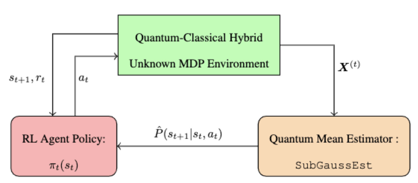
Figure 1: Hybrid Q-Environment architecture depicting agent’s interaction at round $t$ with state $s_{t}\in\mathcal{S}$.

As described in Fig. 1, at round $t$, the agent plays an action $a_{t}$ based on current state $s_{t}$ according to its policy $\pi:\mathcal{S}\rightarrow\mathcal{A}$. Consequently, the unknown MDP Q-environment shares the next state information and reward i.e., $\{s_{t+1},r_{t}\}$. Additionally, it gives the agent access to a set of $S\triangleq|\mathcal{S}|$ quantum random variables, $\bm{X}^{(t)}=\{X_{1}^{(t)},\ldots,X_{|\mathcal{S}|}^{(t)}\}$. Further, every $X_{s}^{(t)}$ is a q.r.v. corresponding to the next state using indicator signals at round $t$. This q.r.v. is corresponding to the random variable:

$$X_{s}^{(t)}\triangleq\bm{1}[s_{t+1}=s]$$ (2)

This q.r.v. can be defined in a Hilbert space $\mathcal{H}$ which has the unitary transformation $U|\mathbf{0}\rangle$ defined as follows:

$$U|\mathbf{0}\rangle= \sqrt{1-P(s_{t+1}=i|s_{t},\leavevmode\nobreak\ a_{t})}|0\rangle$$

$$\leavevmode\nobreak\ \leavevmode\nobreak\ \leavevmode\nobreak\ +\sqrt{P(s_{t+1}=i|s_{t},\leavevmode\nobreak\ a_{t})}|1\rangle,$$ (3)

where $|0\rangle$, $|1\rangle$ are the basis vectors of $\mathcal{H}$. Essentially, $\bm{X}^{(t)}$ could be carefully engineered from quantum representations of the next state. Formally, it is possible to construct the quantum next states can be constructed for the ${S}$ states using $S$ qubits. As an example, state numbered as “1” is encoded as $|10\cdots 0\rangle$, and so on with the last state numbered as “${S}$” encoded by $|0\cdots 01\rangle$. Finally, the overall quantum next state is obtained by quantum vector superposition of these $S$ states with the amplitudes as $\sqrt{P(s_{t+1}=1|s_{t},\leavevmode\nobreak\ a_{t})},\cdots,\sqrt{P(s_{t+1}=S|s_{t},\leavevmode\nobreak\ a_{t})}$, respectively. We highlight that our construction of aforementioned set of quantum indicator variables is key to RL agent’s learning the environment’s transition dynamics governed by probabilities $\{P(\cdot|s,a)\}_{s\in\mathcal{S},a\in\mathcal{A}}$. In our algorithmic framework, we present how the q.r.v. set $\bm{X}^{(t)}$ is carefully integrated with the Quantum Mean Estimator SubGaussEst outlined in Lemma 1 which in turn improves transition probability estimation and leads to exponentially better regret.

RL regret formulation: Consider the RL agent following some policy $\pi:\mathcal{S}\rightarrow\mathcal{A}$ on the unknown MDP Q-environment $\mathcal{M}$. Then, as a result of playing policy $\pi$, the agent’s long term average reward is given by:

$$\Gamma_{\pi}^{P}=\lim_{T\rightarrow\infty}\mathbb{E}_{\pi,P}\big{[}\frac{1}{T}\sum_{t=0}^{T-1}\leavevmode\nobreak\ r(s_{t},a_{t})\big{]},$$ (4)

where $\mathbb{E}_{\pi,P}[\cdot]$ is the expectation taken over the trajectory $\{(s_{t},a_{t})\}_{t\in[0,T-1]}$ by playing policy $\pi$ at every time step. In this context, we state the definitions of value function for MDP $\mathcal{M}$ next:

$$V_{\pi}^{{P}}(s;\gamma) =\mathbb{E}_{a\sim\pi}\Big{[}Q_{\pi}^{{P}}(s,a;\gamma)\Big{]},$$ (5)

$$=\mathbb{E}_{a\sim\pi}\Big{[}r(s,a)+\gamma\sum_{s^{\prime}\in\mathcal{S}}P(s^{\prime}|s,a)V_{\pi}^{{P}}(s^{\prime};\gamma)\Big{]}$$ (6)

Then, according to Puterman (2014), $\Gamma_{\pi}^{P}$ can be represented as the following:

$$\Gamma_{\pi}^{P} =\lim_{\gamma\rightarrow 1}(1-\gamma)V_{\pi}^{{P}}(s;\gamma),\leavevmode\nobreak\ \forall s\in\mathcal{S},$$ (7)

$$=\sum_{s\in\mathcal{S}}\sum_{a\in\mathcal{A}}\rho_{\pi}^{P}(s,a)\overline{r}(s,a),$$ (8)

wherein, $V_{\pi}^{P}(\cdot;\cdot)$ is the discounted cumulative average reward by following policy $\pi$, $\rho_{\pi}^{P}$ is the steady-state occupancy measure (i.e., $\rho_{\pi}^{P}(s,a)\in[0,1],\leavevmode\nobreak\ \sum_{s\in\mathcal{S}}\sum_{a\in\mathcal{A}}\rho_{\pi}^{P}(s,a)=1$). In the following, we introduce key assumptions crucial from the perspective of our algorithmic framework and its analysis. In this context, we introduce the notations $\{P_{\pi,s}^{t},T_{\pi,\leavevmode\nobreak\ s\rightarrow s^{\prime}}\}$ to denote the $t$ time step probability distribution obtained by playing policy $\pi$ on the unknown MDP $\mathcal{M}$ starting from some arbitrary state $s\in\mathcal{S}$; and, the actual time steps to reach $s^{\prime}$ from $s$ by playing policy $\pi$ respectively. With these notations, we introduce our first assumption pertaining to ergodicity of MDP $\mathcal{M}$.

Assumption 1 (Finite MDP mixing time)

We assume that unknown MDP environment $\mathcal{M}$ has finite mixing time, which mathematically implies:

$$T_{\texttt{mix}}\triangleq\max_{\pi,(s,s^{\prime})\in\mathcal{S}\times\mathcal{S}}\leavevmode\nobreak\ \mathbb{E}[T_{\pi,\leavevmode\nobreak\ s\rightarrow s^{\prime}}]<\infty,$$ (9)

where $T_{\pi,\leavevmode\nobreak\ s\rightarrow s^{\prime}}$ implies the number of time steps to reach a state $s^{\prime}$ from an initial state $s$ by playing some policy $\pi$.

Assumption 2

The reward function $r(\cdot,\cdot)$ is known to the RL agent.

We emphasize that Assumption 2 is a commonly used assumption in RL algorithm development owing to the fact that in most setups rewards are constructed according to the underlying problem and is known beforehand Azar et al. (2017); Agarwal et al. (2019). Next, we define the cumulative regret accumulated by the agent in expectation across $T$ time steps as follows:

$$\mathcal{R}_{[0,T-1]}\triangleq T.\Gamma_{\pi^{*}}^{P}-\mathbb{E}\Big{[}\sum_{t=0}^{T-1}r(s_{t},a_{t})\Big{]},$$ (10)

where the agent generates the trajectory $\{(s_{t},a_{t}\}_{t\in[0,T-1]}$ by playing policy $\pi$ on $\mathcal{M}$, and $\pi^{*}$ is the optimal policy that maximizes the long term average reward defined in eq (4). Finally, the RL agent’s goal is to determine a policy $\pi$ which minimizes $\mathcal{R}_{[0,T-1]}$.

4 Algorithmic Framework

In this section, we first delineate the key intuition behind our methodology followed by formal description of Q-UCRL algorithm. If the agent was aware of the true transition probability distribution $P$, then it would simply solve the optimization problem $\bm{\Xi}$ described next.

$$\bm{\Xi}: \max_{\{\rho(s,a)\}_{(s,a)\in\mathcal{S}\times\mathcal{A}}}\leavevmode\nobreak\ \sum_{(s,a)\in\mathcal{S}\times\mathcal{A}}r(s,a)\rho(s,a),$$ (11)

$$\leavevmode\nobreak\ \leavevmode\nobreak\ \text{s.t.},$$ (12)

$$\sum_{(s,a)\in\mathcal{S}\times\mathcal{A}}\rho(s,a)=1,$$ (13)

$$\sum_{a\in\mathcal{A}}\rho(s^{\prime},a)=\sum_{(s,a)\in\mathcal{S}\times\mathcal{A}}P(s^{\prime}|s,a)\rho(s,a),\forall s^{\prime}\in\mathcal{S},$$ (14)

$$\rho(s,a)\geq 0,\forall(s,a)\in\mathcal{S}\times\mathcal{A},$$ (15)

Note that the objective of $\bm{\Xi}$ in eq (11) resembles the definition of steady-state average reward formulation in eq (4). Furthermore, eq (13), (14) preserve the properties of the transition model. Consequently, once it obtains $\{\rho^{*}(s,a)\}_{(s,a)\in\mathcal{S}\times\mathcal{A}}$ by solving $\bm{\Xi}$, it can compute the optimal policy as:

$$\pi^{*}(a|s)=\frac{\rho^{*}(s,a)}{\sum_{\tilde{a}\in\mathcal{A}}\rho^{*}(s,\tilde{a})}$$ (16)

However, in the absence of knowledge pertaining to true $P$, we propose to solve an optimistic version of $\bm{\Xi}$ that will update RL agent’s policy in epochs. Specifically, at the start of an epoch $e$, the following optimization problem will be solved:

$$\tilde{\bm{\Xi}}_{e}: \max_{\{\rho(s,a),P_{e}(\cdot|s,a)\}_{(s,a)\in\mathcal{S}\times\mathcal{A}}}\leavevmode\nobreak\ \sum_{(s,a)\in\mathcal{S}\times\mathcal{A}}r(s,a)\rho(s,a),$$ (17)

$$\leavevmode\nobreak\ \leavevmode\nobreak\ \text{s.t.},$$ (18)

$$\sum_{(s,a)\in\mathcal{S}\times\mathcal{A}}\rho(s,a)=1,$$ (19)

$$\sum_{s^{\prime}\in\mathcal{S}}P_{e}(s^{\prime}|s,a)=1,\leavevmode\nobreak\ \forall(s,a)\in\mathcal{S}\times\mathcal{A},$$ (20)

$$\sum_{a\in\mathcal{A}}\rho(s^{\prime},a)=\sum_{(s,a)\in\mathcal{S}\times\mathcal{A}}{P}_{e}(s^{\prime}|s,a)\rho(s,a),\forall s^{\prime}\in\mathcal{S},$$ (21)

$$\|{P}_{e}(\cdot|s,a)-\hat{P}_{e}(\cdot|s,a)\|_{1}\leq\frac{7S\log(S^{2}At_{e})}{\max\{1,N_{e}(s,a)\}}$$ (22)

$$\rho(s,a)\geq 0,\leavevmode\nobreak\ P_{e}(\cdot|s,a)\geq 0,\leavevmode\nobreak\ \forall(s,a)\in\mathcal{S}\times\mathcal{A}.$$ (23)

Observe that $\tilde{\bm{\Xi}}_{e}$ increases the search space for policy in a carefully computed neighborhood of certain transition probability estimates $\hat{P}$ via eq (22) at the start of epoch $e$. Therfore, solving $\tilde{\bm{\Xi}}_{e}$ is equivalent to obtaining an optimistic policy as it extends the search space of original problem $\bm{\Xi}$. Further, computation of $\hat{P}_{e}$ is key to our framework design as it integrates quantum signals set $\{\bm{X}_{\tau}\}_{\tau\in[1,t_{e}]}$, and their frequencies $\{N_{e}(s,a)\}$ collected upto epoch $e$ to obtain the transition probability estimates via SubGaussEst (SGE) quantum mean estimator defined in Lemma 1.

$$\hat{P}(\cdot|s,a)=\texttt{SGE}(\{X_{\tau}(s,a,s^{\prime})\}_{\tau\in[1,t_{e}]},N_{e}(s,a),\delta_{e})$$ (24)

In Appendix A, we show that $\tilde{\bm{\Xi}}_{e}$ is a convex optimization problem, therefore standard optimization solvers can be employed to solve it. Finally, the agent’s policy at the start of epoch $e$ is given by:

$$\pi_{e}(a|s)=\frac{\rho_{e}(s,a)}{\sum_{\tilde{a}\in\mathcal{A}}\rho_{e}(s,\tilde{a})}$$ (25)

Next, we formally present our method Q-UCRL in Algorithm 1.

Algorithm 1 Q-UCRL

1:Inputs: $\mathcal{S}$, $\mathcal{A}$, $r(\cdot,\cdot)$.

2:Set $t\leftarrow 1,\leavevmode\nobreak\ e\leftarrow 1$

3:Set $\mu(s,a,s^{\prime})\leftarrow 0\leavevmode\nobreak\ \forall(s,a,s^{\prime})\in\mathcal{S}\times\mathcal{A}\times\mathcal{S}$.

4:for $(s,a)\in\mathcal{S}\times\mathcal{A}$ do

5:     Set $\nu_{e}(s,a)\leftarrow 0,\leavevmode\nobreak\ N_{e}(s,a)\leftarrow 0,\leavevmode\nobreak\ \delta_{e}\leftarrow 0,t_{e}\leftarrow 0$.

6:end for

7:Obtain $\pi_{e}$ by solving $\tilde{\bm{\Xi}}_{e}$ and then using eq (25).

8:for $t=1,2,\dots$ do

9:     Observe state $s_{t}$ and play action $a_{t}\sim\pi_{e}(\cdot|s_{t})$.

10:     Observe $s_{t+1},r(s_{t},a_{t})$ and q.r.v realizations $\bm{X}_{t}$.

11:     Update $\nu_{e}(s_{t},a_{t})\leftarrow\nu_{e}(s_{t},a_{t})+1$.

12:     Update $\mu(s_{t},a_{t},s_{t+1})\leftarrow\nu_{e}(s_{t},a_{t},s_{t+1})+1$.

13:     Set $t_{e}\leftarrow t_{e}+1$.

14:     if $\nu_{e}(s_{t},a_{t})=\max\{1,N_{e}(s_{t},a_{t})\}$ then

15:         for $(s,a)\in\mathcal{S}\times\mathcal{A}$ do

16:              $N_{e+1}(s,a)\leftarrow N_{e}(s,a)+\nu_{e}(s,a)$.

17:         end for

18:         Set $e\leftarrow e+1,\leavevmode\nobreak\ \nu_{e}(s,a)\leftarrow 0,\leavevmode\nobreak\ \delta_{e}\leftarrow\frac{1}{S^{2}At_{e}^{7}}$.

19:         Set $t_{e}\leftarrow 0$.

20:         Obtain $\pi_{e}$ by solving $\tilde{\bm{\Xi}}_{e}$ and then using eq (25).

21:     end if

22:end for

Algorithm 1 proceeds in epochs, and each epoch $e$ contains multiple rounds of RL agent’s interaction with the environment. At each $t$, by playing action $a_{t}$ for insantaneous state $s_{t}$ through current epoch policy $\pi_{e}$, the agent collects next state configuration consisting of classical signals $s_{t+1},r(s_{t},a_{t})$ and quantum stochastic signals $\bm{X}_{t}$. Additionally, the agent keeps track of its visitations to the different states via the variables $\{\nu_{s,a},\mu_{s,a,s^{\prime}}\}$. Note that a new epoch is triggered at Line 13 of algorithm 1 is aligned to the widely used concept of doubling trick used in model-based RL algorithm design. Finally, the empirical visitation counts and probabilities upto epoch $e$, i.e., $\{N_{e+1}(s,a),\hat{P}_{e+1}(s^{\prime}|s,a)\}$ attributes are updated (line 14-18), and the policy is updated via re-solving $\tilde{\bm{\Xi}}_{e}$ from eq 17 - (23) and using eq (25).

5 Theoretical Results

In this section, we characterize the regret accumulated for $T$ rounds by running Q-UCRL in a unknown MDP hybrid Q-Environment. In the following, we first present a crucial result bounding the error accumlated till $e$ epochs between the true transition probabilities $\{P(\cdot|s,a)\}$ and the agent’s estimates $\{P_{e}(\cdot|s,a)\}$.

Lemma 2

Execution of Q-UCRL (Algorithm 1) upto total $e$ epochs comprising $t=1,2,\ldots,t_{e}$ rounds, guarantees that the following holds for confidence parameter $\delta_{e}=\frac{1}{SAt_{e}^{7}}$ with probability at least $1-1/t_{e}^{6}$:

$$\|{P}_{e}(\cdot|s,a)-{P}(\cdot|s,a)\|_{1}\leq\frac{14S\log(S^{2}AT)}{\max\{1,N_{e}(s,a)\}},$$ (26)

$\forall(s,a)\in\mathcal{S}\times\mathcal{A}$, where $\{N_{e}^{k}(s,a)\}$ are the cumulative state-action pair visitation counts upto epoch $e$ as depicted in Line 15 of Algorithm 1, and $\{P(\cdot|s,a),P_{e}(\cdot|s,a)\}$ are the actual and estimated transition probabilities.

Proof  To prove the claim in Eq. (26), note that for an arbitrary pair $(s,a)$ we have:

$$\|{P}_{e}(\cdot|s,a)-{P}(\cdot|s,a)\|_{1}$$ (27)

$$\leq \|{P}_{e}(\cdot|s,a)-\hat{P}_{e}(\cdot|s,a)\|_{1}$$

$$+\|\hat{P}_{e}(\cdot|s,a)-{P}(\cdot|s,a)\|_{1},$$

$$\leq \frac{7S\log(S^{2}At_{e})}{\max\{1,N_{e}(s,a)\}}+\|\hat{P}_{e}(\cdot|s,a)-{P}(\cdot|s,a)\|_{1},$$ (28)

$$= \frac{7S\log(S^{2}At_{e})}{\max\{1,N_{e}(s,a)\}}$$ (29)

$$+\sum_{s^{\prime}\in\mathcal{S}}|\underbrace{\hat{P}_{e}(s^{\prime}|s,a)-{P}(s^{\prime}|s,a)}_{\text{(a)}}|,$$

where Eq. (28) is a direct consequence of constraint eq (22) of optimization problem $\tilde{\bm{\Xi}}_{e}$. Next, in order to analyze (a) in Eq. (29), recall the definition of q.r.v’s $X_{s^{\prime},h}^{k}$ presented in Eq. (2) as an indicator q.r.v allows us to write the following for some arbitrary round $t$:

$$\hat{P}_{e}(s^{\prime}|s,a)=\mathbb{E}_{q,\hat{P}_{e}}[X_{s^{\prime}}|s,a],$$ (30)

$${P}(s^{\prime}|s,a)=\mathbb{E}_{q,{P}}[X_{s^{\prime}}|s,a].$$ (31)

Note that eq (30)-(31) depicts that the transition probabilities are indeed true and estimated means for q.r.v $X_{s^{\prime}}$. Since $X_{s^{\prime}}$ is an indicator q.r.v, it’s variance is: $\sigma^{2}\leq 1$. Next consider the following event:

$$\mathcal{E} =\Bigg{\{}|{\hat{P}_{e}(s^{\prime}|s,a)-{P}(s^{\prime}|s,a)}|$$

$$\leq\frac{7\log(S^{2}At_{e})}{\max\{1,N_{e}(s,a)\}},\forall(s,a,s^{\prime})\in\mathcal{S}\times\mathcal{A}\times\mathcal{S}\Bigg{\}},$$ (32)

For a tuple $(s,a,s^{\prime})$, by replacing $\delta=e^{-\epsilon\cdot N_{e}(s,a)}$ into eq (1) from Lemma 1, we get:

$$\mathbb{P}\left[|{\hat{P}_{e}(s^{\prime}|s,a)-{P}(s^{\prime}|s,a)}|\leq\epsilon\right]\geq 1-e^{-\epsilon\cdot N_{e}(s,a)},$$ (33)

By plugging in $\epsilon=\frac{\log(S^{2}At_{e}^{7})}{N_{e}(s,a)}$ into eq (33), we get:

$$\mathbb{P}\left[|{\hat{P}_{e}(s^{\prime}|s,a)-{P}(s^{\prime}|s,a)}|\geq\frac{\log(S^{2}At_{e}^{7})}{N_{e}(s,a)}\right]\leq\frac{1}{S^{2}At_{e}^{7}},$$ (34)

Finally, we sum over all possible values of $N_{e}(s,a)$ as well as tuples $(s,a,s^{\prime})$ to bound the probability in the RHS of (34) that implies failure of event $\mathcal{E}$:

$$\sum_{(s,a,s^{\prime})\in\mathcal{S}\times\mathcal{A}\times\mathcal{S}}\sum_{N_{e}(s,a)=1}^{t_{e}}\frac{1}{S^{2}At_{e}^{7}}\leq\frac{1}{t_{e}^{6}}$$ (35)

Here, it is critical to highlight that we obtain this high probability bound for model errors by careful utilization of Lemma 1 and quantum signals $\bm{X}_{t}$ via eq (30) - (35), while avoiding classical concentration bounds for probability norms that use martingale style analysis such as in the work Weissman et al. (2003). Finally, plugging the bound of term (a) as described by event $\mathcal{E}$, we obtain the following with probability $1-1/t_{e}^{6}$:

$$\|{P}_{e}(\cdot|s,a)-{P}(\cdot|s,a)\|_{1}$$

$$\leq\frac{7S\log(S^{2}At_{e})}{\max\{1,N_{e}(s,a)\}}+\sum_{s^{\prime}\in\mathcal{S}}\frac{\log(S^{2}At_{e}^{7})}{\max\{1,N_{e}(s,a)\}},$$ (36)

$$\leq\frac{7S\log(S^{2}At_{e})}{\max\{1,N_{e}(s,a)\}}+\sum_{s^{\prime}\in\mathcal{S}}\frac{7\log(S^{2}At_{e})}{\max\{1,N_{e}(s,a)\}},$$ (37)

$$=\frac{14S\log(S^{2}At_{e})}{\max\{1,N_{e}(s,a)\}}\leq\frac{14S\log(S^{2}AT)}{\max\{1,N_{e}(s,a)\}}.$$ (38)

This proves the claim as in the statement of the Lemma.  

Remark 1

Note that for probability vectors ${P}_{e}(\cdot|s,a),{P}(\cdot|s,a)$ we have the bound: $\|{P}_{e}(\cdot|s,a)-{P}(\cdot|s,a)\|_{1}\leq 2S$, in the worst case scenario. However, the probability that a bad event (i.e., complementary of eq (26)) happens is at most $\frac{1}{t_{e}^{6}}$.

Regret Decomposition: Regret of Q-UCRL defined in eq (10) can be decomposed as follows:

$$\mathcal{R}_{[0,T-1]} =T.\Gamma_{\pi^{*}}^{P}-\mathbb{E}\Big{[}\sum_{t=0}^{T-1}r(s_{t},a_{t})\Big{]},$$ (39)

$$=T.\Gamma_{\pi^{*}}^{P}-\sum_{e=1}^{E}T_{e}\Gamma_{\pi^{*}_{e}}^{P}$$

$$+\sum_{e=1}^{E}T_{e}\Gamma_{\pi^{*}_{e}}^{P}-\mathbb{E}\Big{[}\sum_{t=0}^{T-1}r(s_{t},a_{t})\Big{]},$$ (40)

$$=\sum_{e=1}^{E}T_{e}\big{(}\underbrace{\Gamma_{\pi^{*}}^{P}-\Gamma_{\pi^{*}_{e}}^{P}}_{\text{(a)}}\big{)}$$

$$+\sum_{e=1}^{E}T_{e}\Gamma_{\pi^{*}_{e}}^{P}-\mathbb{E}\Big{[}\sum_{t=0}^{T-1}r(s_{t},a_{t})\Big{]},$$ (41)

$$=\sum_{e=1}^{E}T_{e}\Gamma_{\pi^{*}_{e}}^{P}-\mathbb{E}\Big{[}\sum_{t=0}^{T-1}r(s_{t},a_{t})\Big{]},$$ (42)

$$\leq\sum_{e=1}^{E}T_{e}\Gamma_{\pi_{e}}^{{P}_{e}}-\mathbb{E}\Big{[}\sum_{t=0}^{T-1}r(s_{t},a_{t})\Big{]},$$ (43)

$$=\sum_{e=1}^{E}T_{e}\Gamma_{\pi_{e}}^{{P}_{e}}-\sum_{e=1}^{E}T_{e}\Gamma_{\pi_{e}}^{{P}}$$

$$+\sum_{e=1}^{E}T_{e}\Gamma_{\pi_{e}}^{{P}}-\mathbb{E}\Big{[}\sum_{t=0}^{T-1}r(s_{t},a_{t})\Big{]},$$ (44)

$$=\sum_{e=1}^{E}T_{e}\Gamma_{\pi_{e}}^{{P}_{e}}-\sum_{e=1}^{E}T_{e}\Gamma_{\pi_{e}}^{{P}}$$

$$+\Big{[}\sum_{e=1}^{E}\sum_{t=t_{e-1}+1}^{t_{e}}\underbrace{\Gamma_{\pi_{e}}^{{P}}-\mathbb{E}[r(s_{t},a_{t})]}_{\text{(}b)}\Big{]},$$ (45)

$$=\sum_{e=1}^{E}T_{e}\Big{(}\Gamma_{\pi_{e}}^{\tilde{P}_{e}}-\Gamma_{\pi_{e}}^{{P}}\Big{)}.$$ (46)

Firstly, (a) in eq (41) is 0 owing to the fact that the agent would have gotten $\pi_{e}^{*}$ exactly as the true $\pi^{*}$ in epoch $e$ solving for original problem $\bm{\Xi}$, had it known the true transition model $P$. Next, eq (43) is because $\{P_{e},\pi_{e}\}$ are outputs from the optimistic problem $\tilde{\bm{\Xi}}_{e}$ solved at round $e$, which extends the search space of $\bm{\Xi}$ and therefore always upper bounds true long-term rewards. Finally, term (b) in eq (45) is 0 in expectation, because the RL agent actually collects rewards by playing policy $\pi_{e}$ against the true $P$ during epoch $e$.

Regret in terms of Bellman Errors: Here, we introduce the notion of Bellman errors $B_{\pi}^{{P}_{e}}(s,a)$ at epoch $e$ as follows:

$$B_{\pi}^{{P}_{e}}(s,a)\triangleq\lim_{\gamma\rightarrow 1} \leavevmode\nobreak\ [Q_{\pi}^{{P}_{e}}(s,a;\gamma)-r(s,a)$$

$$-\gamma\sum_{s^{\prime}\in\mathcal{S}}P(s^{\prime}|s,a)V_{\pi}^{{P}_{e}}(s;\gamma)],$$ (47)

which essentially captures the gap in the average rewards by playing action $a$ in state $s$ accordingly to some policy $\pi$ in one step of the optimistic transition model $P_{e}$ w.r.t. the actual probabilities $P$. This leads us to the following key results that connect the regret expression in eq (46) and the Bellman errors.

Lemma 3

[ Lemma 5.2, Agarwal et al. (2022b)] The difference in long-term expected reward by playing optimistic policy of epoch $e$, i.e., $\pi_{e}$ on the optimistic transition model estimates, i.e., $\Gamma_{\pi_{e}}^{{P}_{e}}$, and the expected reward collected by playing $\pi_{e}$ on the actual model $P$, i.e., $\Gamma_{\pi_{e}}^{{P}}$ is the long-term average of the Bellman errors. Mathematically, we have:

$$\Gamma_{\pi_{e}}^{{P}_{e}}-\Gamma_{\pi_{e}}^{{P}}=\sum_{s,a}\rho_{\pi_{e}}^{P}(s,a)B_{\pi_{e}}^{{P}_{e}}(s,a),$$ (48)

where $B_{\pi}^{{P}_{e}}(s,a)$ is defined in eq (47).

With eq (47), it necessary to mathematically bound the Bellman errors. To this end, we leverage the following result that characterizes the Bellman errors in terms of $\tilde{h}(\cdot)$, a quantity that measures the bias contained in the optimistic MDP model.

Lemma 4

[Lemma 5.3, Agarwal et al. (2022b)] The Bellman errors for any arbitrary state-action pair $(s,a)$ corresponding to epoch $e$ is bounded as follows:

$$B^{\pi_{e},{P}_{e}}(s,a)\leq\Big{\|}{P}_{e}(\cdot|s,a)-{P}(\cdot|s,a)\Big{\|}_{1}\|\tilde{h}(\cdot)\|_{\infty},$$ (49)

where $\tilde{h}(\cdot)$ (defined in Puterman (2014)) is the bias of the optimistic MDP $P_{e}$ for which the optimistic policy $\pi_{e}$ obtains the maximum expected reward in the confidence interval.

Consequently, by plugging in the bound of the error arising from estimation of transition model in Lemma 2 into eq 49, we obtain the following result with probability $1-1/t_{e}^{6}$:

$$B^{\pi_{e},{P}_{e}}(s,a)\leq\frac{14S\log(S^{2}AT)}{\max\{1,N_{e}(s,a)\}}\|\tilde{h}(\cdot)\|_{\infty},$$ (50)

Consequently, it is necessary to bound the model bias error term in eq (50). We recall that the optimistic MDP $P_{e}$ corresponding to epoch $e$ maximizes the average reward in the confidence set as described in the formulation of $\tilde{\bm{\Xi}}_{e}$. In other words, $\Gamma_{\pi_{e}}^{P_{e}}\geq\Gamma_{\pi_{e}}^{P^{\prime}}$ for every $P^{\prime}$ in the confidence interval. Specifically, the model bias for optimistic MDP can be explicitly defined in terms of Bellman equation Puterman (2014), as follows:

$$\tilde{h}(s) \triangleq r_{\pi_{e}}(s)-\lambda_{\pi_{e}}^{P_{e}}+\Big{(}P_{e,\pi_{e}}(\cdot|s)\Big{)}^{T}\tilde{h}(\cdot),$$ (51)

where the following simplified notations are used: $r_{\pi_{e}}(s)=\sum_{a\in\mathcal{A}}\pi_{e}(a|s)r(s,a)$, $P_{e,\pi_{e}}(s^{\prime}|s)=\sum_{a\in\mathcal{A}}\pi_{e}(a|s)P_{e}(s^{\prime}|s,a)$. Next, we incorporate the following result that correlates model bias $\tilde{h}(\cdot)$ to the mixing time $T_{\texttt{mix}}$ of MDP $\mathcal{M}$.

Lemma 5

[Lemma D.5, Agarwal et al. (2022b)] For an MDP with the transition model $P_{e}$ that generates rewards $r(s,a)$ on playing policy $\pi_{e}$, the difference of biases for states $s$ and $s^{\prime}$ are bounded as:

$$\tilde{h}(s)-\tilde{h}(s^{\prime})\leq T_{\texttt{mix}},\forall s,s^{\prime}\in\mathcal{S}.$$ (52)

Plugging in the bound of bias term $\tilde{h}(\cdot)$ into eq (50), we get the final bound for Bellman error with probability $1-1/T^{6}$ as:

$$B^{\pi_{e},\tilde{P}_{e}}(s,a)\leq\frac{14S\log(S^{2}AT)}{\max\{1,N_{e}(s,a)\}}T_{\texttt{mix}}.$$ (53)

Regret Bound for Q-UCRL We now present the final bound for regret incurred by Q-UCRL over a $T$ length training horizon.

Theorem 1

In an unknown MDP environment $\mathcal{M}\triangleq(\mathcal{S},\mathcal{A},P,r,D)$, the regret incurred by Q-URL (Algorithm 1) across $T$ rounds is bounded as follows:

$$\mathcal{R}_{[0,T-1]}=\mathcal{O}\Bigg{(}{S^{3}A^{2}T_{\texttt{mix}}\log^{2}(S^{2}AT)}\Bigg{)}.$$ (54)

Proof  Using the final expression from regret decomposition, i.e., eq (46), we have:

$$\mathcal{R}_{[0,T-1]} =\sum_{e=1}^{E}T_{e}\Big{(}\Gamma_{\pi_{e}}^{\tilde{P}_{e}}-\Gamma_{\pi_{e}}^{{P}}\Big{)},$$ (55)

$$=\frac{1}{T}\sum_{e=1}^{E}\sum_{t=t_{e-1}+1}^{t_{e}}\sum_{s,a}\rho_{\pi_{e}}^{P}B^{\pi_{e},{P}_{e}}(s,a),$$ (56)

$$\leq\sum_{e=1}^{E}\sum_{t=t_{e-1}+1}^{t_{e}}\frac{14S\log(S^{2}AT)}{\max\{1,N_{e}(s_{t},a_{t})\}}T_{\texttt{mix}},$$ (57)

$$=\sum_{e=1}^{E}\sum_{t=t_{e-1}+1}^{t_{e}}\sum_{s,a}\Big{(}\mathbf{1}[s_{t}=s,a_{t}=a]\cdot$$

$$\hskip 28.45274pt\frac{14S\log(S^{2}AT)}{\max\{1,N_{e}(s,a)\}}T_{\texttt{mix}}\Big{)}\Big{)},$$ (58)

$$=\sum_{e=1}^{E}\sum_{s,a}14\nu_{e}(s,a)T_{\texttt{mix}}\frac{S\log(S^{2}AT)}{\max\{1,N_{e}(s,a)\}},$$ (59)

$$=\sum_{s,a}14T_{\texttt{mix}}S\log(S^{2}AT)\sum_{e=1}^{E}\frac{\nu_{e}(s,a)}{\max\{1,N_{e}(s,a)\}},$$ (60)

$$\leq\sum_{s,a}14T_{\texttt{mix}}S\log(S^{2}AT)E,$$ (61)

$$={14}S^{2}AT_{\texttt{mix}}\log(S^{2}AT)E,$$ (62)

$$\leq{14}S^{2}AT_{\texttt{mix}}\log(S^{2}AT)\cdot$$

$$\hskip 28.45274pt(1+2SA+SA\log(T/SA)),$$ (63)

$$=\mathcal{O}\Bigg{(}{S^{3}A^{2}T_{\texttt{mix}}\log^{2}(S^{2}AT)}\Bigg{)}.$$ (64)

where in eq (56), we directly incorporate the result of Lemma 3. Next, we obtain eq (57) by using the Bellman error bound in eq (53), as well as unit sum property of occupancy measures Puterman (2014). Furthermore, in eq. (57) note that we have omitted the regret contribution of bad event (Remark 1) which is atmost $\tilde{\mathcal{O}}\Bigg{(}\frac{2ST_{\texttt{mix}}}{T^{4}}\Bigg{)}$ as obtained below:

$$\sum_{e=1}^{E} \sum_{t=t_{e-1}+1}^{t_{e}}\frac{2ST_{\texttt{mix}}}{t_{e}^{6}}\leq\sum_{e=1}^{E}\frac{2ST_{\texttt{mix}}}{t_{e}^{5}},$$ (65)

$$\leq\sum_{t_{e}=1}^{T}\frac{2ST_{\texttt{mix}}}{t_{e}^{5}}=\tilde{\mathcal{O}}\Bigg{(}\frac{2ST_{\texttt{mix}}}{T^{4}}\Bigg{)}.$$ (66)

Subsequently, eq (59) - (60) are obtaining by using the definition of epoch-wise state-action pair visitation frequencies $\nu_{e}(s,a)$ and the epoch termination trigger condition in Line 13 of Algorithm 1. Finally, we obtain eq (63) by the using Proposition 18 in Appendix C.2 of Auer et al. (2008).  

Remark 2

We reiterate that our characterization of regret incurred by Q-UCRL in Theorem 1 is a martingale-free analysis and thus deviates from its classical counterparts Fruit et al. (2018); Auer et al. (2008); Agarwal et al. (2022b).

6 Conclusions and Future Work

This paper demonstrates that quantum computing helps provide significant reduction in the regret bounds for infinite horizon reinforcement learning with average rewards. This paper not only unveils the quantum potential for bolstering reinforcement learning but also beckons further exploration into novel avenues that bridge quantum and classical paradigms, thereby advancing the field to new horizons.

We note that this paper considers a model-based setup, while model-free setup for the problem is an important problem for the future.

Appendix A Appendix A: Convexity of Optimization Problem

In order to solve the optimistic optimization problem described by $\tilde{\bm{\Xi}}_{e}$ for epoch $e$ (eq (17) - (23)), we adopt the approach proposed in Agarwal et al. (2022b); Rosenberg and Mansour (2019). The key is that the constraint in (21) seems non-convex. However, that can be made convex with an inequality as

$$\sum_{a\in\mathcal{A}}\rho(s^{\prime},a)\leq\sum_{(s,a)\in\mathcal{S}\times\mathcal{A}}{P}_{e}(s^{\prime}|s,a)\rho(s,a),\leavevmode\nobreak\ \forall s^{\prime}\in\mathcal{S}$$ (67)

This makes the problem convex since $xy\geq c$ is convex region in the first quadrant.

However, since the constraint region is made bigger, we need to show that the optimal solution satisfies (21) with equality. This follows since

$$\sum_{s^{\prime}\in\mathcal{S}}\sum_{(s,a)\in\mathcal{S}\times\mathcal{A}}{P}_{e}(s^{\prime}|s,a)\rho(s,a)=1=\sum_{s^{\prime}\in\mathcal{S}}\sum_{a\in\mathcal{A}}\rho(s^{\prime},a)$$ (68)

Thus, since we have point-wise inequality in (67) with the sum of the two sides being the same, thus, the equality holds for all $s^{\prime}$.

Appendix B Appendix B: A brief overview of Quantum Amplitude Amplification

Quantum amplitude amplification stands as a critical outcome within the realm of quantum mean estimation. This pivotal concept empowers the augmentation of the amplitude associated with a targeted state, all the while suppressing the amplitudes linked to less desirable states. The pivotal operator, denoted as $Q$, embodies the essence of amplitude amplification: $Q=2|\psi\rangle\langle\psi|-I$, where $|\psi\rangle$ signifies the desired state and $I$ represents the identity matrix. This operator orchestrates a double reflection of the state $|\psi\rangle$ - initially about the origin and subsequently around the hyperplane perpendicular to $|\psi\rangle$ - culminating in a significant augmentation of the amplitude of $|\psi\rangle$.

Moreover, the application of this operator can be iterated to achieve a repeated amplification of the desired state’s amplitude, effectively minimizing the amplitudes of undesired states. Upon applying the amplitude amplification operator a total of $t$ times, the outcome is $Q^{t}$, which duly enhances the amplitude of the desired state by a scaling factor of $\sqrt{N}/M$, where $N$ corresponds to the overall count of states and $M$ signifies the number of solutions.

The implications of quantum amplitude amplification extend across a diverse spectrum of applications within quantum algorithms. By bolstering their efficacy and hastening the resolution of intricate problems, quantum amplitude amplification carves a substantial niche. Noteworthy applications encompass:

1. Quantum Search: In the quantum algorithm for unstructured search, known as Grover’s algorithm Grover (1996), the technique of amplitude amplification is employed to enhance the amplitude of the target state and decrease the amplitude of the non-target states. As a result, this technique provides a quadratic improvement over classical search algorithms.
   

2. Quantum Optimization: Quantum amplification can be used in quantum optimization algorithms, such as Quantum Approximate Optimization Algorithm (QAOA) Farhi et al. (2014), to amplify the amplitude of the optimal solution and reduce the amplitude of sub-optimal solutions. This can lead to an exponential speedup in solving combinatorial optimization problems.
   

3. Quantum Simulation: Quantum amplification has also been used in quantum simulation algorithms, such as Quantum Phase Estimation (QPE) Kitaev (1995), to amplify the amplitude of the eigenstate of interest and reduce the amplitude of other states. This can lead to an efficient simulation of quantum systems, which is an intractable problem in the classical domain.
   

4. Quantum Machine Learning: The utilization of quantum amplification is also evident in quantum machine learning algorithms, including Quantum Support Vector Machines (QSVM) Lloyd et al. (2013). The primary objective is to amplify the amplitude of support vectors while decreasing the amplitude of non-support vectors, which may result in an exponential improvement in resolving particular classification problems.

In the domain of quantum Monte Carlo methods, implementing quantum amplitude amplification can enhance the algorithm’s efficiency by decreasing the amount of samples needed to compute the integral or solve the optimization problem. By amplifying the amplitude of the desired state, a substantial reduction in the number of required samples can be achieved while still maintaining a certain level of accuracy, leading to significant improvements in efficiency when compared to classical methods. This technique has been particularly useful in Hamoudi (2021) for achieving efficient convergence rates in quantum Monte Carlo simulations.

References

- Agarwal et al. (2019) Alekh Agarwal, Nan Jiang, Sham M Kakade, and Wen Sun. Reinforcement learning: Theory and algorithms. CS Dept., UW Seattle, Seattle, WA, USA, Tech. Rep, 32, 2019.
- Agarwal and Aggarwal (2023) Mridul Agarwal and Vaneet Aggarwal. Reinforcement learning for joint optimization of multiple rewards. Journal of Machine Learning Research, 24(49):1–41, 2023.
- Agarwal et al. (2022a) Mridul Agarwal, Vaneet Aggarwal, and Tian Lan. Multi-objective reinforcement learning with non-linear scalarization. In Proceedings of the 21st International Conference on Autonomous Agents and Multiagent Systems, pages 9–17, 2022a.
- Agarwal et al. (2022b) Mridul Agarwal, Qinbo Bai, and Vaneet Aggarwal. Concave utility reinforcement learning with zero-constraint violations. Transactions on Machine Learning Research, 2022b.
- Agrawal and Jia (2017) Shipra Agrawal and Randy Jia. Optimistic posterior sampling for reinforcement learning: worst-case regret bounds. Advances in Neural Information Processing Systems, 30, 2017.
- Al-Abbasi et al. (2019) Abubakr O Al-Abbasi, Arnob Ghosh, and Vaneet Aggarwal. Deeppool: Distributed model-free algorithm for ride-sharing using deep reinforcement learning. IEEE Transactions on Intelligent Transportation Systems, 20(12):4714–4727, 2019.
- Auer et al. (2008) Peter Auer, Thomas Jaksch, and Ronald Ortner. Near-optimal regret bounds for reinforcement learning. Advances in neural information processing systems, 21, 2008.
- Azar et al. (2017) Mohammad Gheshlaghi Azar, Ian Osband, and Rémi Munos. Minimax regret bounds for reinforcement learning. In International Conference on Machine Learning, pages 263–272. PMLR, 2017.
- Biamonte et al. (2017) Jacob Biamonte, Peter Wittek, Nicola Pancotti, Patrick Rebentrost, Nathan Wiebe, and Seth Lloyd. Quantum machine learning. Nature, 549(7671):195–202, 2017.
- Bonjour et al. (2022) Trevor Bonjour, Marina Haliem, Aala Alsalem, Shilpa Thomas, Hongyu Li, Vaneet Aggarwal, Mayank Kejriwal, and Bharat Bhargava. Decision making in monopoly using a hybrid deep reinforcement learning approach. IEEE Transactions on Emerging Topics in Computational Intelligence, 6(6):1335–1344, 2022.
- Bouland et al. (2023) Adam Bouland, Yosheb M Getachew, Yujia Jin, Aaron Sidford, and Kevin Tian. Quantum speedups for zero-sum games via improved dynamic gibbs sampling. In International Conference on Machine Learning, pages 2932–2952. PMLR, 2023.
- Brassard et al. (2002) Gilles Brassard, Peter Hoyer, Michele Mosca, and Alain Tapp. Quantum amplitude amplification and estimation. Contemporary Mathematics, 305:53–74, 2002.
- Casalé et al. (2020) Balthazar Casalé, Giuseppe Di Molfetta, Hachem Kadri, and Liva Ralaivola. Quantum bandits. Quantum Machine Intelligence, 2:1–7, 2020.
- Chen et al. (2021) Jiayu Chen, Abhishek K Umrawal, Tian Lan, and Vaneet Aggarwal. Deepfreight: A model-free deep-reinforcement-learning-based algorithm for multi-transfer freight delivery. In Proceedings of the International Conference on Automated Planning and Scheduling, volume 31, pages 510–518, 2021.
- Dunjko et al. (2017) Vedran Dunjko, Jacob M Taylor, and Hans J Briegel. Advances in quantum reinforcement learning. In 2017 IEEE International Conference on Systems, Man, and Cybernetics (SMC), pages 282–287. IEEE, 2017.
- Farhi et al. (2014) Edward Farhi, Jeffrey Goldstone, and Sam Gutmann. A quantum approximate optimization algorithm. arXiv preprint arXiv:1411.4028, 2014.
- Fruit et al. (2018) Ronan Fruit, Matteo Pirotta, Alessandro Lazaric, and Ronald Ortner. Efficient bias-span-constrained exploration-exploitation in reinforcement learning. In International Conference on Machine Learning, pages 1578–1586. PMLR, 2018.
- Ganguly et al. (2023) Bhargav Ganguly, Yulian Wu, Di Wang, and Vaneet Aggarwal. Quantum computing provides exponential regret improvement in episodic reinforcement learning. arXiv preprint arXiv:2302.08617, 2023.
- Gilyén et al. (2019) András Gilyén, Yuan Su, Guang Hao Low, and Nathan Wiebe. Quantum singular value transformation and beyond: exponential improvements for quantum matrix arithmetics. In Proceedings of the 51st Annual ACM SIGACT Symposium on Theory of Computing, pages 193–204, 2019.
- Grover (1996) Lov K Grover. A fast quantum mechanical algorithm for database search. In Proceedings of the twenty-eighth annual ACM symposium on Theory of computing, pages 212–219, 1996.
- Hamoudi (2021) Yassine Hamoudi. Quantum sub-gaussian mean estimator. arXiv preprint arXiv:2108.12172, 2021.
- Harrow et al. (2009) Aram W Harrow, Avinatan Hassidim, and Seth Lloyd. Quantum algorithm for linear systems of equations. Physical review letters, 103(15):150502, 2009.
- Jerbi et al. (2021) Sofiene Jerbi, Lea M Trenkwalder, Hendrik Poulsen Nautrup, Hans J Briegel, and Vedran Dunjko. Quantum enhancements for deep reinforcement learning in large spaces. PRX Quantum, 2(1):010328, 2021.
- Kitaev (1995) A Yu Kitaev. Quantum measurements and the abelian stabilizer problem. arXiv preprint quant-ph/9511026, 1995.
- Lloyd et al. (2013) Seth Lloyd, Masoud Mohseni, and Patrick Rebentrost. Quantum algorithms for supervised and unsupervised machine learning. arXiv preprint arXiv:1307.0411, 2013.
- Montanaro (2015) Ashley Montanaro. Quantum speedup of monte carlo methods. Proceedings of the Royal Society A: Mathematical, Physical and Engineering Sciences, 471(2181):20150301, 2015.
- Osband et al. (2013) Ian Osband, Daniel Russo, and Benjamin Van Roy. (more) efficient reinforcement learning via posterior sampling. Advances in Neural Information Processing Systems, 26, 2013.
- Paparo et al. (2014) Giuseppe Davide Paparo, Vedran Dunjko, Adi Makmal, Miguel Angel Martin-Delgado, and Hans J Briegel. Quantum speedup for active learning agents. Physical Review X, 4(3):031002, 2014.
- Puterman (2014) Martin L Puterman. Markov decision processes: discrete stochastic dynamic programming. John Wiley & Sons, 2014.
- Rosenberg and Mansour (2019) Aviv Rosenberg and Yishay Mansour. Online convex optimization in adversarial markov decision processes. In International Conference on Machine Learning, pages 5478–5486. PMLR, 2019.
- Silver et al. (2017) David Silver, Julian Schrittwieser, Karen Simonyan, Ioannis Antonoglou, Aja Huang, Arthur Guez, Thomas Hubert, Lucas Baker, Matthew Lai, Adrian Bolton, et al. Mastering the game of go without human knowledge. nature, 550(7676):354–359, 2017.
- Sutton and Barto (2018) Richard S Sutton and Andrew G Barto. Reinforcement learning: An introduction. MIT press, 2018.
- Wang et al. (2021a) Daochen Wang, Aarthi Sundaram, Robin Kothari, Ashish Kapoor, and Martin Roetteler. Quantum algorithms for reinforcement learning with a generative model. In International Conference on Machine Learning, pages 10916–10926. PMLR, 2021a.
- Wang et al. (2021b) Daochen Wang, Xuchen You, Tongyang Li, and Andrew M Childs. Quantum exploration algorithms for multi-armed bandits. In Proceedings of the AAAI Conference on Artificial Intelligence, volume 35, pages 10102–10110, 2021b.
- Weissman et al. (2003) Tsachy Weissman, Erik Ordentlich, Gadiel Seroussi, Sergio Verdu, and Marcelo J Weinberger. Inequalities for the l1 deviation of the empirical distribution. Hewlett-Packard Labs, Tech. Rep, 2003.