^†^†thanks: CONTACT Jing Li. Email: jingl8@illinois.edu

Treatment bootstrapping: A new approach to quantify uncertainty of average treatment effect estimates

\nameJing Li^a ^aDepartment of Political Science, University of Illinois at Urbana-Champaign, Urbana, IL, USA

Abstract

This paper proposes a new non-parametric bootstrap method to quantify the uncertainty of average treatment effect estimate for the treated from matching estimators. More specifically, it seeks to quantify the uncertainty associated with the average treatment effect estimate for the treated by bootstrapping the treatment group only and finding the counterpart control group by matching on estimated propensity score. We demonstrate the validity of this approach and compare it with existing bootstrap approaches through Monte Carlo simulation and real world data set. The results indicate that the proposed approach constructs confidence interval and standard error that have at least comparable precision and coverage rate as existing bootstrap approaches, while the variance estimates can fluctuate depending on the proportion of treatment group units in the sample data and the specific matching method used.

keywords:

Causal Inference; Average Treatment Effect; Non-parametric Bootstrap; Propensity Score

1 Introduction

Applications of causal inference methods have increased dramatically in the last few decades. In observational studies, because of the non-random assignment of treatment, the treatment and control groups too often are unbalanced on their observed covariates. One way to remedy this problem is through matching (Rosenbaum and Rubin 1983, 1985; Abadie and Imbens 2011; Diamond and Sekhon 2013; Sekhon 2011). While a lot of scholarly attention has duly been focused on estimating the average treatment effect (ATE) using different matching estimators, the equally important issue of the uncertainty of average treatment effect estimates has been emphasized much less. This is reflected in the fact that there is a fair amount of variation and ambiguity in how applied causal inference research derives and reports uncertainty of average treatment effect estimates. While most studies do report standard error or confidence interval (Aldrich and Kage 2011; Boas and Hidalgo 2011; Dehejia 2002; Galiani et al. 2005; Gerber and Green 2005; Hong and Park 2016; Kam and Palmer 2008; Kocher et al 2011; Mayer 2011; Mozer et al 2020; Simmons and Hopkins 2005; Urban and Niebler 2014), only a minority of these ones mention which specific method is used (Dehejia 2002; Galiani et al. 2005; Gerber and Green 2005; Mayer 2011; Urban and Niebler 2014).

This often leaves readers unsure how uncertainty measures of ATE estimates are derived. And even if the name of a particular method is mentioned, the bootstrap method for example, readers are still unsure of the specific steps taken to form the uncertainty measures. In this paper, we explore uncertainty measures for ATE estimates and more specifically uncertainty measures derived from the non-parametric bootstrap method.

While the non-parametric bootstrap method and its rich array of variants and extensions are common ways to derive standard error or confidence interval for ATE estimates especially for matching estimators, a closer scrutiny of this method in practice is still much needed in the literature. In particular, in this paper, we propose a new way of quantifying uncertainty of average treatment effect for the treated (ATT) estimates, compare it with existing methods, and discuss their relative strengths and weaknesses. In addition, while real-world experiments can be carried out, often they are time-consuming and demand a large amount of financial, administrative, and other resources. So while researchers can design the best possible experiment for their specific research question, it’s rarely the case that they have the luxury to replicate experiments in multiple different settings. Therefore, analytically quantifying the uncertainty of ATT estimates has real-world significance.

The paper is organized as follows: section 2 briefly reviews the potential outcome framework for causal inference; section 3 discusses the uncertainty of ATE estimates; section 4 reviews relevant existing bootstrap approaches and provides details on the proposed non-parametric bootstrap approach for deriving standard error and confidence interval of sample ATT estimate; section 5 presents simulation studies and results; section 6 offers discussions and conclusions.

2 Causal Inference and Causal Effect Estimation

The fundamental problem in causal inference is that we cannot observe a unit in its factual and counter-factual states at the same time. Therefore, for two potential outcomes $Y_{i}(1)$ and $Y_{i}(0)$ , a unit can only be either treated or not treated at a specific point in time but not both at the same time (Holland 1986). Obtaining the counter-factual state for either treated or control units necessitates removing the effect of all factors on potential outcomes other than that of the treatment. The Neyman-Rubin causal model shifts the problem of causal effect identification and inference to estimating the average treatment effect (ATE) between two comparable treatment and control groups (Rubin 1974, 1978). That is:

ATE=E(Y_{i}(1)-Y_{i}(0))=E(Y_{i}\mid T=1)-E(Y_{i}\mid T=0)

(1)

Randomized experiment treatment assignment balances both observed and unobserved covariates between the treatment group and control groups, thus making the treatment and control groups comparable, obtaining counter-factual states for both treatment and control, and enabling estimation of the average treatment effect as a result. That is:

ATE=E(Y_{i}\mid T=1)-E(Y_{i}\mid T=0)=\frac{1}{n_{t}}\sum_{i=1}^{n_{t}}Y_{i}-\frac{1}{n_{c}}\sum_{i=1}^{n_{c}}Y_{i}

(2)

When randomized treatment assignment doesn’t exist as in observational settings, statistical adjustment methods such as matching are needed to account for the non-random assignment of treatment, identify the counter-factual states, and enable estimation of the average treatment effect(Diamond and Sekhon 2013; Hansen 2004). More specifically, we may estimate the average treatment effect for the treated (ATT) and the average treatment effect for the control (ATC):

ATT=E((Y_{i}(1)-Y_{i}(0))|T=1)=E(Y_{i}(1)|T=1)-E(Y_{i}(0)|T=1)

(3)

ATC=E((Y_{i}(1)-Y_{i}(0))|T=0)=E(Y_{i}(1)|T=0)-E(Y_{i}(0)|T=0)

(4)

When treatment assignment is randomized, potential outcomes have statistical independence with treatment assignment, and $ATE=ATT=ATC$ , otherwise $ATE$ does not equal $ATT$ or $ATC$ in general. In this paper, we focus on $ATT$ .

3 Uncertainty of Causal Effect Estimate

While the uncertainty of treatment effect estimates has been acknowledged by statisticians since the early days in the development of the causal inference framework(Fisher, R.A. 1935; Neyman 1923), in applied studies, researchers seem to have a tendency to gloss over this important component of the causal inference process. In applied settings, while it is common that standard error or confidence interval of the ATE estimate is provided, often times no details are presented on exactly how they are derived (Abadie and Gardeazabal 2003; Aldrich and Kage 2011; Boas and Hidalgo 2011; Christakis and Iwashyna 2003; Dehejia 2002; Diamond and Sekhon 2013; Galiani et al. 2005; Gerber and Green 2005; Hansen 2004; Hong and Park 2016; Kam and Palmer 2008; Kocher et al 2011; Mayer 2011; Mozer et al 2020; Simmons and Hopkins 2005; Urban and Niebler 2014).

In a number of studies, names of the procedure used, for example ”bootstrap”, are mentioned (Dehejia 2002; Galiani et al. 2005; Gerber and Green 2005; Mayer 2011; Urban and Niebler 2014), but again no details are given. This often leave readers wonder precisely how the standard errors or confidence intervals are derived. In a few other works, uncertainty of causal effect estimates are not addressed at all (Abadie, Diamond and Hainmueller 2010; Henderson and Chatfield 2011). Notable exceptions are Rosenbaum (2002) which constructs confidence interval of treatment effect estimates by inverting hypothesis tests and collecting all values not rejected at a certain $\alpha$ level into a confidence set, and Abadie and Imbens (2002); Imbens (2004) which offer an analytic solution for deriving the variance of ATE estimates.

Therefore, developing the best practice for quantifying the uncertainty of ATE estimates is still much needed and it is just as important as estimating ATE in the first place. And while in certain cases researchers have derived mathematical expressions for variance estimators for certain specific ATE estimators (Imbens and Rubin 2015; Rojas 2009), these analytical solutions do not serve more general use cases and often are not intuitive to understand.

Then, how can we quantify the inherent uncertainty associated with ATE estimates? In discussing the different approaches used for deriving confidence interval for treatment effect estimated from propensity score matching: normal-theory approaches, resampling approaches, and randomization-based approaches, Hill and Reiter (2006) shows that bootstrap-based methods have superior performance compared with other methods in certain situations. In the following, we also propose a non-parametric bootstrap approach for measuring uncertainty associated with ATT estimates.

4 Non-parametric Bootstrapping of Average Treatment Effect for the Treated (ATT)

4.1 Existing bootstrap approaches for quantifying uncertainty of ATE estimates

The bootstrap method as first introduced by Efron (Efron 1979) is a non-parametric approach to quantify the uncertainty of parameter estimates when there is not much information about the population distribution of parameter of interest. The key principle is to re-sample from an original data sample with replacement, which produces replicated resample data with desired random variation naturally embedded in it, thus enabling us to form uncertainty measures such as standard error or confidence interval. The rationale behind the bootstrap procedure is that the bootstrap distribution of $\tilde{\tau}-\hat{\tau}$ closely mimics the sampling distribution of $\hat{\tau}-\tau$ , known as the bootstrap Central Limit Theorem (Singh 1981).

However, bootstrap is not a one-fits-all method and it can fail for certain types of data and for certain types of statistics¹¹1The formal conditions where the bootstrap generally work are: for any distribution $A$ within a neighborhood of the true distribution F, the bootstrap distribution $G_{A,n}$ converges weakly to a limiting distribution $G_{A,\infty}$ ; this convergence is uniform on the neighborhood; and the mapping from $A$ to $G_{A,\infty}$ must be continuous (Bickel and Freedman 1981; Davison and Hinkley 1997).. Cases where the bootstrap can fail include when the statistic of interest is the sample maximum, unstable or unsmooth statistic, for example, the sample median (Bickel and Freedman 1981; Davison and Hinkley 1997), or when the parameter lies on the boundary of the parameter space (Andrews, W.K. Donald 2000); or the bootstrap can fail when the sample data in question has dependence structure, for example, auto-correlated time series data, incomplete data, or dirty data (Davison and Hinkley 1997). Therefore, when leveraging the bootstrap method to quantify uncertainty associated with the average treatment effect estimate, cautions ought to be observed.

For matching estimators more specifically, Abadie and Imbens (2008) show that the standard bootstrap in general is not valid for simple nearest-neighbor matching with replacement and a fixed number of neighbors ²²2They do point out that for asymptotically linear estimators such as propensity score pair-matching without replacement, the bootstrap method does provide valid inference., while they provide analytical asymptotic variance estimators for matching estimators with replacement and a fixed number of matches (Abadie and Imbens 2006) and propensity score matching with replacement (Abadie and Imbens 2016). Abadie and Spiess (2022) shows that a matched bootstrap, which resamples matched sets of one treatment unit and K control units without replacement, does provide valid standard errors of average treatment effect estimate. In addition, Bodory et al. (2020) shows that a wild bootstrap procedure, which is based on a martingale representation of matching estimators proposed by Abadie and Imbens (2012), performs well compared with standard bootstrap and (conservative) asymptotic variance approximations. Otsu and Rai (2017) proposes a weighted bootstrap approach by directly taking the number of times a unit is used for matching as an attribute of the unit when bootstrapping ³³3This inference method is for matching with replacement.. Austin and Small (2014) show the validity of a paired bootstrap procedure which bootstraps pairs of matched treatment and control units. Our proposed approach follows this line of work, and more specifically bootstraps the sample treatment group first and then construct the counterpart control group by pair matching on estimated propensity score without replacement, and does not contradict with results of Abadie and Imbens (2008).

4.2 A comparison of different bootstrap ATE approaches

Below we make a comparison between the proposed approach and three most commonly used bootstrapping procedures for deriving uncertainty measures of average treatment effect estimates. These three approaches all use the bootstrap method to derive the standard error of average treatment effect estimate from propensity score matching⁴⁴4That is the matching procedure first estimates a conditional probability (propensity score) to be treated for each one of the treatment and control group units and then match treatment and control group units on estimated propensity score.. The first kind of bootstrap is to bootstrap the sample treatment group and control groups separately (Hall and Marin 1988; Tu and Zhou 2002; Abadie and Imbens 2008; Peng 2011); the second one is a paired bootstrap which bootstraps a pair of treatment and control units after performing pair matching on estimated propensity score without replacement on the sample data, with matched pair of treatment and control units staying with each other during the bootstrap process (Austin and Small 2014); the third and most common type is to bootstrap the entire sample of both treatment and control units together (Austin and Stuart 2017; Austin 2022; Cerulli 2014; Bodory et al. 2020) ⁵⁵5We specifically refer to the standard bootstrap in (Bodory et al. 2020). Other than these three bootstrap approaches listed, there are possibly a lot more non-parametric bootstrap methods that have been used to derive uncertainty measures of average treatment effect estimates for matching estimators. However, the focus of this paper will be on these three approaches as they are easy to understand and comparison between the proposed approach and these three basic approaches can shed light on the statistical properties of other variants of bootstrap uncertainty measures. In addition, as most applied causal inference work using the bootstrap method to derive standard error or confidence interval of ATE estimates does not report exactly how the bootstrap procedure is done, chances are there are many more applied works that use the three basic bootstrap approaches listed above than the ones cited here.. In this paper, we only consider matching without replacement and compare the three bootstrap approaches listed above with the proposed approach described below.

Embens and Menzel. (2021) differentiates between uncertainty from sampling variation and uncertainty from the stochastic nature of the treatment assignment. To adjudicate among the four different bootstrap approaches, it is also helpful to examine what kind of uncertainty or randomness they are trying to identify and estimate. The paired bootstrap approach by Austin and Small (2014) resamples pairs of matched treatment and control group units. It can be argued that a pair of treatment and control group units represents an individual treatment effect estimated from a treatment group unit and its matched control group counterpart, that is Austin and Small (2014) is essentially bootstrapping individual treatment effects. Therefore, the main uncertainty accounted for by the paired bootstrap approach is how individual treatment effect could vary across the sample treatment units. The matched set bootstrap approach in Abadie and Spiess (2022) can be seen as an extended version of the paired bootstrap where the number of control units matched to a treatment unit will not necessarily be 1.

When bootstrapping sample treatment and control groups separately, we are accounting for both the uncertainty associated with the treatment group and the uncertainty associated with the control group, but do it separately. In other words, we are accounting for two sources of uncertainty at the same time yet not in a principled way. For one thing, treatment assignment is unlikely to be random or independent of the observed covariates in an observational setting, therefore, there could be overlaps between uncertainty associated with the treatment group and uncertainty associated with the control group. And accounting for the two sources of uncertainty separately could potentially overestimate the uncertainty of sample treatment effect estimates. In other words, the crude way of bootstrapping treatment and control groups separately could provide biased uncertainty estimate for average treatment effect estimate because the two sources of uncertainty are not accounted for in any principled way.

When bootstrapping the entire sample data including both the treatment group and the control group, we are accounting for the uncertainty associated with the sample data (of both treatment and control units) as a whole. Therefore, it does not necessarily identify and estimate the specific uncertainty associated with the average treatment effect estimate. In one bootstrap step, the number of treatment group units, the number of control group units, the composition of the treatment group, and the composition of the control group all can change at the same time. However, that is not how we would expect treatment effect to vary in the real world ⁶⁶6Again Embens and Menzel. (2021) characterizes two types of uncertainty and one simple bootstrap of the whole sample data cannot account for both at the same time.. In a real world setting, the most simple way to think about how treatment effect estimate can vary is to form many randomized experiments⁷⁷7More specifically, in the real world, in an experimental setting, we would expect the people who receive treatment will change with each experiment, and the corresponding control group also changes such that it matches the treatment group (in both observed and unobserved covariates) as the pair of treatment group and control group comes from one randomized experiment.. And in observational settings, to mimic the construction of many experiments, we would like to create many matched pairs of treatment and control groups.

The question is how best to construct many matched pairs of treatment and control groups to mimic randomized experiments as close as possible from observational data. In this paper, we take a very specific perspective on the uncertainty associated with average treatment effect estimate. For matching estimators of ATT more specifically, our starting point is the sample treatment group. Therefore, to accurately identify and estimate the uncertainty of ATT estimate, we should start with accounting for the uncertainty associated with the treatment group first and then address uncertainty associated with subsequent steps of matching and specifically the uncertainty associated with matched control group. To specifically account for the uncertainty associated with the treatment group, we can just perform a simple bootstrap step. And to account for the uncertainty associated with the control group, we can just pair-match control group units with bootstrap resample treatment group units on estimated propensity score, exactly same matching procedure as how we obtain the ATT estimate for the sample data. In other words, we are not strictly addressing the sampling variation and treatment assignment variation as outlined by Embens and Menzel. (2021), but we are addressing the same two sources of uncertainties involved in the same process in a different and simple way.

We focus on ATT because when we try to identify and estimate the average treatment effect, the expectation is that the treatment in question will have a causal effect on the outcome of interest for those that are treated and not have an effect for the control. Therefore, we are most interested in how the average treatment effect can vary for those that are treated. By bootstrapping the sample treatment group only, we are capturing the type of uncertainty that really matters for the average treatment effect estimate. Moreover, the proposed approach also remedies a problem commonly encountered in bootstrap inference for average treatment effect estimate (Abadie and Imbens 2008; Otsu and Rai 2017), that is units in the sample data appear only once while a bootstrap resample treatment group will almost surely contain certain sample data units more than once. Therefore, if we are to find the exact matched counterpart control group for a bootstrap treatment group resample such that these two groups mimic a randomized experiment as close as possible, we will not be able to find any because the sample control group doesn’t have any units that appear more than once. Our proposed approach to match bootstrap resample treatment group with sample control group on estimated propensity score remedies this issue. A pair of bootstrapped resample treatment group and its matched counterpart control group can serve as a close approximation to a randomized experiment ⁸⁸8In social demographic as well as other settings, individuals subject to a certain treatment or intervention normally is a small group while the potential control pool is quite large, therefore, in general, there should be sufficient number of control units available to match with the treatment group units as demonstrated below in a simulation exercise using the CPS data set..

The detailed procedure of how we derive the bootstrapped average treatment effect estimates (for matching estimators) is as follows:

Non-parametric Bootstrapped Average Treatment Effect Estimate:

Step 1. Calculate a propensity score for each of the units in the sample data set using the logit model (the dependent variable is the treatment indicator, the predictors are covariate variables other than the treatment indicator and the outcome $Y$ : $\text{pscore}=\frac{e^{p}}{1+e^{p}},~{}p=\beta_{0}+\sum_{i=1}^{n_{c}}\beta_{i}x_{i}$ , the number of covariates);

Step 2. Match a set of units from the sample control group to the sample treatment group based on estimated propensity score from step 1 ⁹⁹9We are matching without replacement, if a unit in the control pool gets matched to a treatment unit, it will not be considered when finding matches for other treatment units.;

Step 3. Compute the ATT estimate by calculating the mean difference of the outcome $Y$ between the treatment group and the matched control group;

Step 4. Bootstrap the treatment group (sample same-size with replacement) 1000 times to obtain 1000 bootstrap resamples, repeat steps 2 and 3 to find matched control group counterpart for each bootstrap treatment group resample¹⁰¹⁰10This ensures that the matched counterpart control group for each bootstrapped resample treatment group is dynamic. It is superior to the approach of bootstrapping separately the sample treatment group and the sample control group, because here we are primarily dealing with one source of uncertainty that is easy to quantify while bootstrapping both treatment and control groups introduce two sources of randomness at the same time and are difficult to quantify and may very likely produce misleading results. As aforementioned above, the proposed approach accounts for two sources of uncertainties involved in estimating ATT in a different but principled way., and calculate an ATT estimate for each pair of bootstrap treatment group resample and its matched control group.

4.3 Validity of the proposed bootstrap method

Consider a basic setup where we have $X,Y,Z$ denoting different random variables. $Z$ is a binary treatment indicator, for example, participation in a job training program, $Z=1$ for the treatment group and $Z=0$ for the control group. $Y$ is the outcome variable, $X$ refers to the $p\times 1$ set of covariates for both the treatment and control groups (for example, demographic variables such as race, education, income, gender, age, etc.). The question of interest is to estimate the effect of the treatment on the outcome for units in the treated group.

Let us define $\tau$ as the population statistic of interest, namely average treatment effect for the treated, the sample ATT estimate as $\hat{\tau}$ , and bootstrap resample ATT estimate as $\tilde{\tau}$ . For the bootstrap method, the assumption is that the distribution of $\tilde{\tau}-\hat{\tau}$ can approximate the distribution of $\hat{\tau}-\tau$ well. Suppose the sample size of the matched sample is $n$ . If we assume $\sqrt{n}(\hat{\tau}-\tau)\to_{d}N(0,\sigma^{2})$ for some $\sigma>0$ , then $\sqrt{n}(\tilde{\tau}-\hat{\tau})\to_{d}N(0,\sigma^{2})$ .

As is common in the literature, we adopt a few assumptions that will enable us to establish the validity of the proposed bootstrap approach.

Assumption 1 (random sampling): sample data $S=\{Y_{i},X_{i},Z_{i}\}^{N}_{i=1}$ consists of $N_{1}$ treatment and $N_{0}$ control units, which are random draws from the population distribution $(Y,X)$ for the treated ( $Z=1$ ) and control $Z=0$ respectively, so $N=N_{1}+N_{0}$ . And let $S^{\ast}\subseteq S$ be the matched sample obtained via pair-matching without replacement on estimated propensity score $\gamma_{i}=f(Z_{i},X_{i})$ ¹¹¹¹11Estimated propensity score is just one way of summarizing the information of $X$ values, therefore, theoretically speaking, alternative matching metrics such as Mahalanobis distance could potentially work with the proposed approach as well..

Assumption 2 (common support condition): let $\Gamma_{1}=supp(\gamma|z=1)$ , and $\Gamma_{0}=supp(\gamma|z=0)$ , then $\Gamma_{1}\subseteq\Gamma_{0}$ . This ensures that enough good matches from the control group can be found for the treatment group units.

Assumption 3 (matching discrepancies): with $N_{0}>>N_{1}$ , the assumption is that regardless of which specific matching algorithm being used, the procedure will be able to ensure that $X_{1}$ and $X_{0}$ of the matched sample have close enough distributions.

Matching as a type of quasi-experimental design creates a matched sample $S^{\ast}$ , which can mimic a randomized experiment and provide a treatment effect estimate. This estimate asymptotically is expected to recover the true treatment effect in the target matching population $P^{\ast}$ , in which the treatment and control groups have same distribution of $X$ . That is ATT estimate $\hat{\tau}$ from the matched sample asymptotically can recover the true treatment effect $\tau$ in the population.

Assumption 4 (unobserved confounding): the assumption is that conditional on observed covariates $X$ , the potential outcome $Y(1)$ and $Y(0)$ is independent of the treatment assignment, $(Y(1),Y(0))\perp Z$ (Rosenbaum and Rubin 1983). However, in order for this to hold, we need to assume that no unobserved confounding exists that systemically biases the relationship between $Y$ and $Z$ .

Let the variance of the bootstrap ATT estimate $\tilde{\tau}$ be $\lambda_{n}(\tilde{\tau})$ , and $n=1000$ , then the bootstrap procedure is said to be valid if $\lambda_{n}(\tilde{\tau})-\lambda_{n}(\hat{\tau})\to_{p}0$ . With the random sampling assumption above and a large enough sample size $n=1000$ , it is typically the case that $\lambda_{n}(\hat{\tau})\to\lambda(\tau)$ . Then to prove that $\lambda_{n}(\tilde{\tau})-\lambda_{n}(\hat{\tau})\to_{p}0$ , we only need $\lambda_{n}(\tilde{\tau})\to_{p}\lambda(\tau)$ . And with $\lambda_{n}(\tilde{\tau})-\lambda_{n}(\hat{\tau})=(\lambda_{n}(\tilde{\tau})-\lambda(\tau))-(\lambda_{n}(\hat{\tau})-\lambda(\tau))$ , we can prove that $\lambda_{n}(\tilde{\tau})-\lambda_{n}(\hat{\tau})\to_{p}0$ ¹²¹²12Let $G_{n}(t)=\lambda_{n}(\hat{\tau})=P(\sqrt{n}(\hat{\tau}-\tau)\leq t),~{}\tilde{G}_{n}(t)=\lambda_{n}(\tilde{\tau})=P(\sqrt{n}(\tilde{\tau}-\hat{\tau})\leq t)$ , using the Berry-Essen theorem, it can be shown that $\underset{t}{\text{supp}}|\tilde{G}_{n}(t)-G_{n}(t)|=O_{p}(1/\sqrt{n})$ , therefore, the bootstrap approach is statistically valid..

Below we demonstrate the validity of the proposed bootstrap approach through a Monte Carlo simulation and a simulation using the Current Population Survey (CPS) data set, and compare it with the main existing alternatives.

5 Simulation Studies

5.1 Monte Carlo Simulation

Here we perform Monte Carlo simulation to examine the behavior of our proposed bootstrap variance estimator and make a comparison with the three alternative approaches discussed above.

In accordance with the random sampling assumption, our sample data are random samples from a super population of size 1000000. The sample size of a random sample from the super population can differ, and we have three different values: 500, 1000, 2000. In addition, the percentage of treatment units in the super population varies across four different scenarios: 5 percent, 10 percent, 20 percent, 25 percent. For each of these four scenarios, random samples of size 500, 1000 and 2000 are generated.

The data generating process of the super population mimics the ones used in the literature Austin and Small (2014); Austin (2022) for a continuous outcome. There are 10 baseline covariates: $X_{1},...,X_{10}$ . These covariates all follow the standard normal distribution. Seven of them $X_{1},...,X_{7}$ affects the treatment assignment and seven of them $X_{4},...,X_{10}$ affects the outcome. And the covariates’ effect on the treatment assignment or the outcome could be weak, medium, strong, or very strong. The probability of treatment is formed from a logit model: $\text{logit}(p_{i})=\alpha_{0,\text{treat}}+\alpha_{w}x_{1}+\alpha_{m}x_{2}+\alpha_{s}x_{3}+\alpha_{w}x_{4}+\alpha_{m}x_{5}+\alpha_{s}x_{6}+\alpha_{vs}x_{7}$ . And the treatment status is generated from a Bernoulli distribution with unit-specific parameter $p_{i}:Z_{i}\sim\text{Bernulli}(p_{i})$ . The continuous outcome was generated from the following formula: $Y_{i}=Z_{i}+\alpha_{w}x_{4}+\alpha_{m}x_{5}+\alpha_{s}x_{6}+\alpha_{vs}x_{7}+\alpha_{w}x_{8}+\alpha_{m}x_{9}+\alpha_{s}x_{1}0+\epsilon_{i}$ , where $\epsilon_{i}\sim N(0,\sigma=3)$ . The true treatment effect is 1, that is the treatment increases the average outcome by one unit.

For each of the sample data, we perform propensity score matching using three different algorithms: optimal matching (with a distance tolerance of 0.02), caliper matching with a caliper of 0.1, and nearest neighbor matching. Therefore, in total, we have 144 different types of results for 12 different data scenarios (4 different ratio of treatment units and 3 different sample size), 3 different matching methods, and 4 different bootstrap methods for deriving ATT uncertainty measures. And the main statistical properties of the uncertainty measures we look at are coverage rate and mean standard error across 1000 iterations for each scenario. The coverage rate refers to the number of times the 95 percent confidence interval ( $\tau-1.96se_{B},\tau+1.96se_{B}$ ) traps the true treatment effect 1, and the mean standard error is the arithmetic mean of 1000 standard errors ( $se_{B}(\tilde{\tau})=\sqrt{\frac{1}{n}\sum_{i=1}^{n}(\tilde{\tau}_{i}-\hat{\tau})^{2}}$ ) calculated from 1000 runs for each scenario.

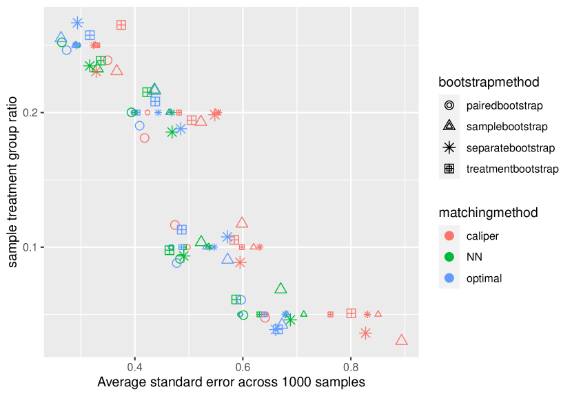
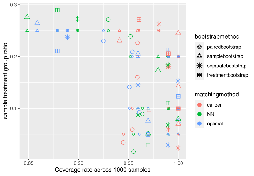
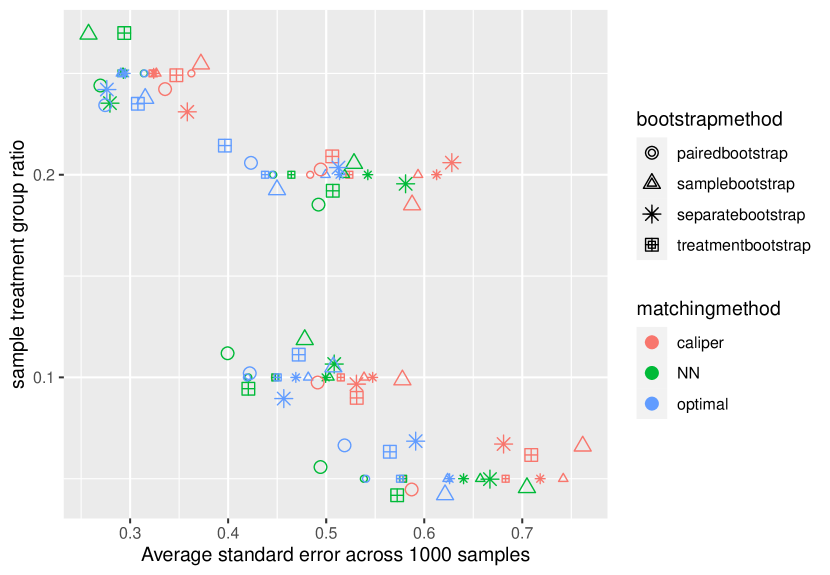
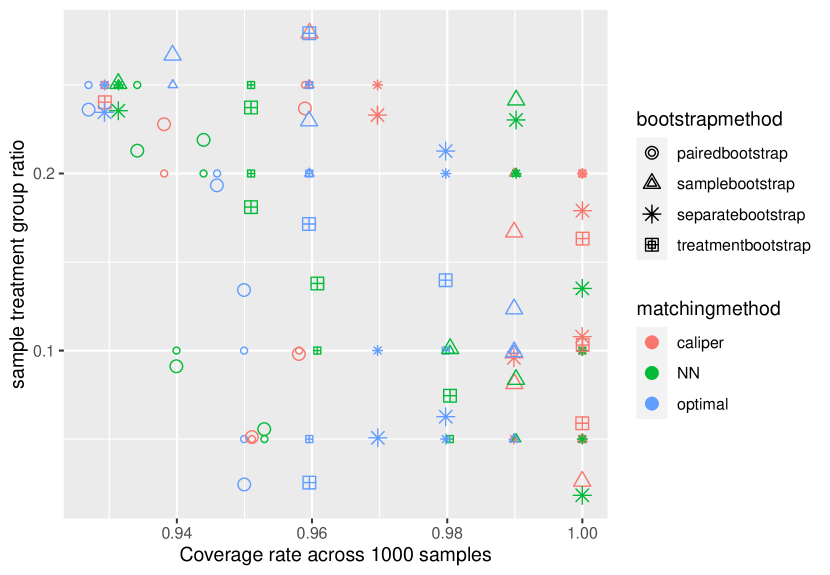
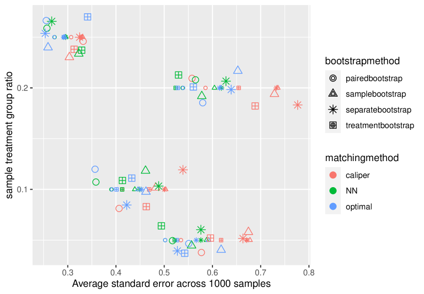
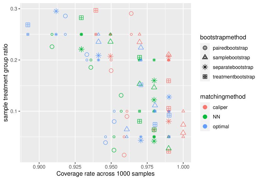
Refer to caption — Figure 1: Mean Standard Error and Coverage Rate for Sample size 500

In Figure 1, 2, and 3 ¹³¹³13The figures are gittered to address overplotting, exact values of mean standard errors as well as coverage rates can be looked up in the Appendix Tables 1, 2, 3., we can observe that both coverage rate and mean standard error decreases as the ratio of treatment group units increases in the sample data for all methods used and all sample sizes, indicating that there seems to be a bias-variance trade-off. When the bias gets smaller, the variance seems to get bigger. In most scenarios our proposed treatment group bootstrap achieves comparable coverage rate and mean standard error compared with the three commonly used bootstrap approaches. Often times it is one of the existing three ones that has the largest mean standard error or smallest coverage rate. There are only 3 occasions where the coverage rate of the proposed approach is below 0.9, around 0.88 when sample sizes are 500 or 2000. Only in one occasion does the approach has larger mean standard error, that is when the sample size is 2000, the treatment units ratio is 0.25 and the matching method is caliper matching. In fact, more often than not along with the paired bootstrap it achieves lower mean standard error compared with the other two approaches.

This provides numerical evidence that the proposed bootstrap approach can form comparable or more precise uncertainty measures for ATT estimate. And the corresponding coverage rates are quite satisfactory, in most cases reaching 95 percent or above. However, there are fluctuations in both mean standard error and coverage rate depending on the ratio of the treatment group in the sample, the specific matching method, and the sample size.

5.2 Simulation with the CPS dataset

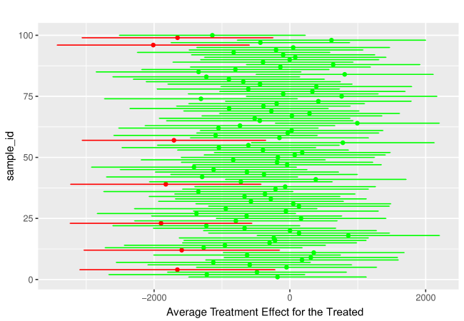
Different from the Monte Carlo simulation above, here we examine the behavior of the proposed bootstrap approach as well as the three existing ones using a real-world data set, the Current Population Study (CPS) data set. First, we randomly assign 175 individuals ¹⁴¹⁴14This treatment group size mimics the Dehejia-Wahha Sample of the Lalonde NSW experiment data (Lalonde 1986). to be the treatment group while the remaining units act as the control group. Repeating this exercise 1000 times gives us 1000 simulated data sets. Applying propensity score matching to each of these 1000 data sets, and we can obtain 1000 pre-bootstrapped average treatment effect estimates. This is the sampling distribution of ATT. As all units in CPS data set are not treated, the average treatment effect estimate should be zero in expectation¹⁵¹⁵15That is the true treatment effect is zero.. The sample mean of the non-bootstrapped ATT is -450.9568 (real earnings in dollars in 1978), which is pretty close to the true treatment effect value of 0, while the standard deviation is 685.1427.

Results displayed in Figure 4 show that the proposed non-parametric bootstrap procedure can quantify the uncertainty of average treatment effect estimate reasonably well. Across 100 runs of the proposed bootstrap procedure for 100 samples (randomly drawn from the 1000 sample data sets generated above), 93 out of the 100 bootstrap confidence intervals trap the true treatment effect of 0, while in 3 of the other 7 cases, the true treatment effect 0 is pretty close to be within two standard errors of the ATT estimate. The green error bars in Figure 4 are those 93 which have 0 within 2 standard errors away from the sample ATT estimate while the red error bars are those 7 which do not have 0 within 2 standard errors away from the sample ATT estimate.

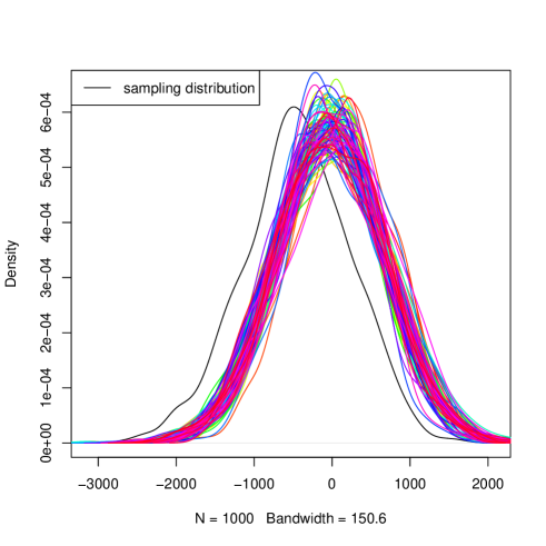
In Figure 5, we plot the sample distribution of ATT, the single black curve on the left, that is the distribution of ATT estimates of the 1000 non-bootstrapped samples, along with 100 bootstrap distributions of ATT, the 100 colored curves on the right, the 100 data samples for which we calculated bootstrapped standard error and 95 percent confidence interval of the sample ATT estimates. It can be observed that the bootstrap distributions are in the same shape as the sample distribution of ATT, the only difference is that the sample distribution is centered slightly to the left.

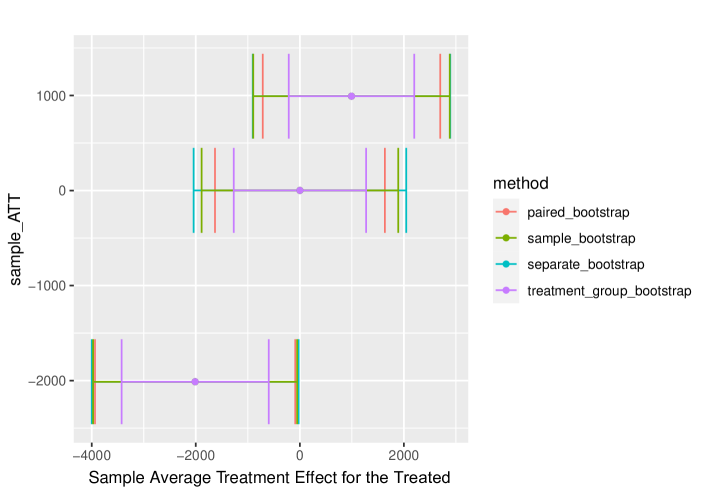
In Figure 6, we show the approximate 95 percent confidence intervals for the proposed bootstrap method as well as the three existing ones for three difference cases of sample ATT: when the sample ATT has the smallest negative value, is closest to zero (the true treatment effect), and has the largest positive value. It can be observed that in all three cases, the proposed approach achieves the narrowest confidence interval. Therefore, the uncertainty measure derived from bootstrapping the treatment group only and pair-matching on estimated propensity score without replacement appears to be more precise than the existing approaches.

6 Discussions and Conclusion

Compared with the existing line of work that uses non-parametric bootstrap to quantify the uncertainty of average treatment effect estimate, our proposed approach of bootstrapping the treatment group only and finding the counterpart control groups by pair matching on estimated propensity score without replacement has shown to be able to provide comparatively precise uncertainty measures for ATT estimates in most scenarios in the Monte Carlo simulation and the simulation using CPS data set above. It also provides high coverage rates. Nonetheless, it is necessary to be aware of the bias-variance trade-off and the potential issue of relatively low coverage rate when it is more difficult to find good matches for treatment group units, that is when the ratio of treatment group units in sample data is relatively big as is demonstrated by the Monte Carlo simulation results above.

In essence, our proposed bootstrap approach tries to account for the two sources of uncertainty involved in estimating ATT in a different but principled way. First, we deal with the variation associated with the treatment group by bootstrapping the treatment group, and then we deal with the variation associated with the matched control group by pair matching the bootstrap treatment group resamaple with the sample control group units on estimated propensity score without replacement. A pair of bootstrap resample treatment group and its corresponding matched control group effectively serves as an approximation to treatment and control groups from a randomized experiment¹⁶¹⁶16If there exists other method that can find the counterpart control group for each bootstrapped treatment group resample such that the pair of matched treatment and control groups more closely mimics a randomized experiment, then we might leverage that method..

In addition, we need to consider other factors that can affect how well the proposed bootstrap approach will work. First, it depends on how common or representative the sample treatment group data is. If the sample data and especially the sample treatment group only represents a rare case to start with, then the proposed non-parametric bootstrap method will not be able to create meaningful estimate of the uncertainty associated with the sample ATT estimate.

Second, in the simulations above, we match individual units in each sample data set based on their estimated propensity score. We acknowledge the fact that matching units on estimated propensity scores is not perfect. While estimated propensity score helps to balance treatment and control group units on observed covariates, it cannot help balance the matched treatment and control group units on unobserved covariates, which brings an element of bias to our proposed bootstrap standard error estimate for the sample ATT.

And lastly, the non-parametric bootstrap approach proposed above is computationally efficient. For both simulation studies above, using a Windows desktop computer with Intel(R) Xeon(R) Platinum 8-score CPU 2.6 GHZ and 32 Gigabyte RAM and the R Matching package, the computation time for each sample of treatment and control groups is around 3-7 minutes across the different matching methods and data scenarios while we implement certain parallel computing mechanisms into our code. With the rapid advances in computing power and availability of distributed computing frameworks such as Apache Spark, we are optimistic that the computation time can be further reduced with the proposed bootstrap approach.

References

Abadie and Gardeazabal (2003) Abadie, Alberto, and Javier, Gardeazabal. (2003). The Economic Costs of Conflict: A Case Study of the Basque Country. The American Economic Review. 2003.
Abadie and Imbens (2002) Abadie, Alberto and Imbens, Guido W. (2002).Simple and Bias-corrected Matching Estimators for average treatment effects. National Bureau of Economic Research 2002; NBER Working Paper Series(283).
Abadie and Imbens (2006) Abadie, Alberto and Imbens, Guido W. (2006). Large Sample Properties of Matching Estimators for Average Treatment Effects. Econometrica, 74(1), 235–267.
Abadie and Imbens (2008) Abadie, Alberto and Imbens, Guido W. (2008). Notes and comments on the failure of the bootstrap for matching estimators. Econometrica, 76(6), 1537–1557.
Abadie and Imbens (2011) Abadie, Alberto and Guido W. Imbens. (2011). Bias-Corrected Matching Estimators for Average Treatment Effects, Journal of Business and Economic Statistics, 29:1, 1-11
Abadie and Imbens (2012) Alberto Abadie and Guido W. Imbens. (2012). A Martingale Representation for Matching Estimators, Journal of the American Statistical Association, 107:498, 833-843.
Abadie and Imbens (2016) Alberto Abadie and Guido W. Imbens. (2016). Matching on Estimated Propensity Score.Econometrica, 84(2), 781-807.
Abadie, Diamond and Hainmueller (2010) Abadie, Alberto, Diamond, Alexis and Hainmueller, Jens. (2010). Synthetic Control Methods for Comparative Case Studies: Estimating the Effect of California’s Tobacco Control Program. Journal of the American Statistical Association, 105(490), 493-505.
Abadie and Spiess (2022) Abadie, Alberto and Spiess, Jann. (2022). Robust Post-Matching Inference, Journal of the American Statistical Association, 117:538, 983-995.
Aldrich and Kage (2011) Aldrich, D., and Kage, R. (2011). Japanese Liberal Democratic Party Support and the Gender Gap: A New Approach. British Journal of Political Science, 41(4), 713-733. Standard errors provided but no details.
Andrews, W.K. Donald (2000) Andrews, W.K. Donald. (2000). Inconsistency of the bootstrap when a parameter is on the boundary of the parameter space. Econometrica, 68(2), 399-405.
Austin and Small (2014) Austin, C.Peter, and Small, S.Dylan. (2014). The use of bootstrapping when using propensity-score matching without replacement: a simulation study. Statistics in Medicine, 33, 4306-4319.
Austin and Stuart (2017) Austin, Peter and Stuart, EA. (2017). Estimating the effect of treatment on binary outcomes using full matching on the propensity score. Stat Methods Med Res, 26(6), 2505-2525.
Austin (2022) Austin, PC. (2022). Bootstrap vs asymptotic variance estimation when using propensity score weighting with continuous and binary outcomes. Statistics in Medicine. 41(22): 4426–4443.
Boas and Hidalgo (2011) Boas, T.C. and Hidalgo, F.D. (2011). Controlling the Airwaves: Incumbency Advantage and Community Radio in Brazil. American Journal of Political Science 55: 869-885.
Bickel and Freedman (1981) Bickel, J. Peter, and Freedman, David. (1981) Some asymptotic theory for the bootstrap. Annals of Statistics, 9(6), 1196-1217.
Bodory et al. (2020) Bodory,Hugo, Lorenzo Camponovo, Martin Huber and Michael Lechner (2020). The Finite Sample Performance of Inference Methods for Propensity Score Matching and Weighting Estimators. Journal of Business and Economic Statistics, 38(1), 183-200.
Embens and Menzel. (2021) Guido Imbens. Konrad Menzel. ”A causal bootstrap.” Ann. Statist. 49 (3) 1460 - 1488, June 2021.
Cerulli (2014) Cerulli, Giovanni. (2014) treatrew: A user-written command for estimating average treatment effects by reweighting on the propensity score. The Stata Journal, 14(3), 541–561.
Christakis and Iwashyna (2003) Christakis, Nicholas A. and Iwashyna, Theodore J.. (2003). The Health Impact of Health Care on Families: A matched cohort study of hospice use by decedents and mortality outcomes in surviving, widowed spouses. Social Science and Medicine, 57(3), 465–475.
Davison and Hinkley (1997) Davison, A.C. and Hinkley, D.V. (1997). Bootstrap Methods and their Application. Cambridge, UK ; New York : Cambridge University Press.
Dehejia (2002) Dehejia, Rajeev H. and Wahba, Sadek. (2002). Propensity Score-matching methods for nonexperimental causal studies. The Review of Economics and Statistics, 84(1), 151–161.
Diamond and Sekhon (2013) Diamond, A. and Sekhon, J.S. Geneticmatching for estimating causal effects: A generalmultivariate matching method for achieving balance in observational studies. (2013). Rev. Econ. Stat. 95. 932–945.
Dynarski (2003) Dynarski, S. M. 2003. Does Aid Matter? Measuring the Effect of Student Aid on College Attendance and Completion. The American Economic Review. 93, 279–288.
Efron (1979) Efron, B. (1979). Bootstrap Methods: Another Look at the Jackknife. Ann. Stat, 7(1), 1-26.
Fisher, R.A. (1935) Fisher, R.A. (1935). The Design of Experiments. Oliver and Boyd. Edinburgh.
Galiani et al. (2005) Galiani, Sebastian, Gertler, Paul and Schargrodsky, Ernesto. (2005). Water for Life: The Impact of the Privatization of Water Services on Child Mortality. Journal of Political Economy, 113(1), 83–120.
Gerber and Green (2005) Gerber, Alan S. and Green, Donald P. (2005). Correction to Gerber and Green (2000), Replication of Disputed Findings, and Reply to Imai (2005) American Political Science Review, 99(2), 301-313.
Hall and Marin (1988) Hall, Peter and Martin, Michael. (1988). On the bootstrap and two-sample problems. Austral. J. Statist. 30A, 179–192.
Hansen (2004) Hansen, B.B. (2004). Full matching in an observational study of coaching for the SAT. J. Amer. Stat. Assoc., 99, 609–618.
Henderson and Chatfield (2011) Henderson, John and Sara, Chatfield. (2011). The Journal of Politics 73:3, 646-658.
Hill and Reiter (2006) Hill J, Reiter JP. (2006). Interval estimation for treatment effects using propensity score matching. Statistics in Medicine 25(13):2230–2256.
Holland (1986) Holland, Paul W. (1986). Statistics and Causal Inference. Journal of the American Statistical Association.
Hong and Park (2016) Hong, J., and Park, S. (2016). Factories for Votes? How Authoritarian Leaders Gain Popular Support Using Targeted Industrial Policy. British Journal of Political Science, 46(3), 501-527.
Imbens (2004) Imbens GW. Nonparametric estimation of average treatment effects under exogeneity: a review. Review of Economics and Statistics 2004; 86:4–29.
Imbens and Rubin (2015) Imbens, Guido and Rubin, Donald. (2015). Causal inference for statistics, social, and biomedical sciences : an introduction. Cambridge University Press.
Imbens and Menzel (2021) Imbens, Guido and Menzel, Konrad. (2021). A Causal Bootstrap. The Annals of Statistics 49(3), 1460-1488.
Kam and Palmer (2008) Cindy D. Kam and Carl L. Palmer. (2008). Reconsidering the Effects of Education on Political Participation. The Journal of Politics 70(3), 612-631.
Kocher et al (2011) Kocher, M.A., Pepinsky, T.B. and Kalyvas, S.N. (2011). Aerial Bombing and Counterinsurgency in the Vietnam War. American Journal of Political Science 55: 201-218.
Lalonde (1986) Lalonde, Robert J. (1986). Evaluating the econometric evaluations of training programs with experimental data. Amer. Econ. Rev., 76(4), 604-620.
Mayer (2011) Mayer, Alexander. 2011. Does Education Increase Political Participation?. The Journal of Politics 73 (3): 633–645.
Mozer et al (2020) Mozer, R., Miratrix, L., Kaufman, A., and Jason Anastasopoulos, L. (2020). Matching with Text Data: An Experimental Evaluation of Methods for Matching Documents and of Measuring Match Quality. Political Analysis 28(4), 445-468.
Neyman (1923) Neyman, J.N. On the application of probability theory to agricultural experiments. Essay on principles. Section 9 (1923), Stat. Sci. 5 (1923 [1990]), pp. 463–480. reprint. Transl. by Dabrowska and Speed.
Otsu and Rai (2017) Taisuke Otsu and Yoshiyasu Rai. (2017). Bootstrap Inference of Matching Estimators for Average Treatment Effects, Journal of the American Statistical Association, 112 (520), 1720-1732.
Rosenbaum and Rubin (1983) Rosenbaum, P.R. and Rubin, Donald B. (1983). The central role of the propensity score in observational studies for causal effects. Biometrika, 70(1), 41-55.
Rosenbaum and Rubin (1985) Rosenbaum, P.R. and Donald B. Rubin (1985) Constructing a Control Group Using Multivariate Matched Sampling Methods That Incorporate the Propensity Score, The American Statistician, 39:1, 33-38.
Rosenbaum (2002) Rosenbaum, P.R. (2002). Observational Studies. Springer. New York.
Rubin (1986) Rubin, Donald B. (1986). Statistics and Causal Inference: Comment: Which Ifs Have Causal Answers. Journal of the American Statistical Association, 81(396), 961-962.
Rubin (1974) Rubin, Donald B. (1974). Estimating causal effects of treatments in randomized and nonrandomized studies. J. Educ. Psychol, 66(5), 688–701.
Rubin (1978) Rubin, Donald B.(1978). Bayesian inference for causal effects: The role of randomization. Ann. Stat, 6(1), 34–58.
Peng (2011) Peng, Xia, Jing, Ping, and Feng, Zi’ou. (2011). Bootstrap Confidence Intervals for the Estimation of Average Treatment Effect on Propensity Score. Journal of Mathematics Research, 3(3), 52:58.
Rojas (2009) Rojas, Gabriel Montes. (2009). A note on the variance of average treatment effects estimators. Economics Bulletin. 29(4), 2937-2943.
Singh (1981) Singh, Kesar. (1981). On the Asymptotic Accuracy of Efron’s Bootstrap. Ann. Stat, 9(6), 1187-1195.
Sekhon (2011) Sekhon, J. S. (2011). Multivariate and Propensity Score Matching Software with Automated Balance Optimization: The Matching package for R. Journal of Statistical Software, 42(7), 1–52.
Simmons and Hopkins (2005) Simmons, B., and Hopkins, D. (2005). The Constraining Power of International Treaties: Theory and Methods. American Political Science Review, 99(4), 623-631.
Tu and Zhou (2002) Tu, Wanzhu, and Zhou, Xiao-Hua. (2002). A Bootstrap Confidence Interval Procedure for the Treatment Effect Using Propensity Score Subclassification. Health Services and Outcomes Research Methodology, 3, 135:147.
Urban and Niebler (2014) Urban, C. and Niebler, S. (2014), Dollars on the Sidewalk: Should U.S. Presidential Candidates Advertise in Uncontested States?. American Journal of Political Science 58: 322-336.

Table 1: Caliper Matching Results

Matching	samplesize	Trtratio	Bootstrap	coverage	sd
caliper	1000	0.05	pairedbootstrap	0.951	0.578
caliper	1000	0.05	samplebootstrap	1.000	0.742
caliper	1000	0.05	separatebootstrap	0.990	0.718
caliper	1000	0.05	treatmentbootstrap	1.000	0.683
caliper	1000	0.10	pairedbootstrap	0.958	0.448
caliper	1000	0.10	samplebootstrap	0.990	0.539
caliper	1000	0.10	separatebootstrap	1.000	0.547
caliper	1000	0.10	treatmentbootstrap	1.000	0.515
caliper	1000	0.20	pairedbootstrap	0.938	0.484
caliper	1000	0.20	samplebootstrap	0.990	0.594
caliper	1000	0.20	separatebootstrap	1.000	0.613
caliper	1000	0.20	treatmentbootstrap	1.000	0.524
caliper	1000	0.25	pairedbootstrap	0.959	0.362
caliper	1000	0.25	samplebootstrap	0.960	0.327
caliper	1000	0.25	separatebootstrap	0.970	0.324
caliper	1000	0.25	treatmentbootstrap	0.929	0.323
caliper	2000	0.05	pairedbootstrap	0.959	0.535
caliper	2000	0.05	samplebootstrap	1.000	0.678
caliper	2000	0.05	separatebootstrap	0.980	0.671
caliper	2000	0.05	treatmentbootstrap	0.990	0.618
caliper	2000	0.10	pairedbootstrap	0.961	0.413
caliper	2000	0.10	samplebootstrap	1.000	0.503
caliper	2000	0.10	separatebootstrap	0.990	0.500
caliper	2000	0.10	treatmentbootstrap	0.990	0.469
caliper	2000	0.20	pairedbootstrap	0.950	0.586
caliper	2000	0.20	samplebootstrap	0.990	0.736
caliper	2000	0.20	separatebootstrap	0.990	0.733
caliper	2000	0.20	treatmentbootstrap	0.990	0.654
caliper	2000	0.25	pairedbootstrap	0.964	0.307
caliper	2000	0.25	samplebootstrap	0.970	0.331
caliper	2000	0.25	separatebootstrap	0.949	0.328
caliper	2000	0.25	treatmentbootstrap	0.939	0.328
caliper	500	0.05	pairedbootstrap	0.945	0.643
caliper	500	0.05	samplebootstrap	1.000	0.850
caliper	500	0.05	separatebootstrap	1.000	0.831
caliper	500	0.05	treatmentbootstrap	0.971	0.762
caliper	500	0.10	pairedbootstrap	0.954	0.498
caliper	500	0.10	samplebootstrap	1.000	0.620
caliper	500	0.10	separatebootstrap	0.990	0.631
caliper	500	0.10	treatmentbootstrap	1.000	0.598
caliper	500	0.20	pairedbootstrap	0.959	0.423
caliper	500	0.20	samplebootstrap	1.000	0.549
caliper	500	0.20	separatebootstrap	0.990	0.555
caliper	500	0.20	treatmentbootstrap	0.990	0.482
caliper	500	0.25	pairedbootstrap	0.959	0.330
caliper	500	0.25	samplebootstrap	0.941	0.327
caliper	500	0.25	separatebootstrap	0.980	0.323
caliper	500	0.25	treatmentbootstrap	0.961	0.331

Table 2: Nearest Neighbor Matching Results

NN	1000	0.05	pairedbootstrap	0.953	0.538
NN	1000	0.05	samplebootstrap	0.990	0.657
NN	1000	0.05	separatebootstrap	1.000	0.640
NN	1000	0.05	treatmentbootstrap	0.980	0.578
NN	1000	0.10	pairedbootstrap	0.940	0.421
NN	1000	0.10	samplebootstrap	0.980	0.503
NN	1000	0.10	separatebootstrap	1.000	0.499
NN	1000	0.10	treatmentbootstrap	0.961	0.448
NN	1000	0.20	pairedbootstrap	0.944	0.446
NN	1000	0.20	samplebootstrap	0.990	0.519
NN	1000	0.20	separatebootstrap	0.990	0.542
NN	1000	0.20	treatmentbootstrap	0.951	0.464
NN	1000	0.25	pairedbootstrap	0.934	0.314
NN	1000	0.25	samplebootstrap	0.931	0.293
NN	1000	0.25	separatebootstrap	0.931	0.293
NN	1000	0.25	treatmentbootstrap	0.951	0.291
NN	2000	0.05	pairedbootstrap	0.952	0.502
NN	2000	0.05	samplebootstrap	0.990	0.588
NN	2000	0.05	separatebootstrap	0.980	0.576
NN	2000	0.05	treatmentbootstrap	0.980	0.522
NN	2000	0.10	pairedbootstrap	0.957	0.390
NN	2000	0.10	samplebootstrap	0.980	0.439
NN	2000	0.10	separatebootstrap	0.980	0.449
NN	2000	0.10	treatmentbootstrap	0.970	0.413
NN	2000	0.20	pairedbootstrap	0.936	0.538
NN	2000	0.20	samplebootstrap	0.970	0.604
NN	2000	0.20	separatebootstrap	0.980	0.619
NN	2000	0.20	treatmentbootstrap	0.970	0.524
NN	2000	0.25	pairedbootstrap	0.909	0.273
NN	2000	0.25	samplebootstrap	0.949	0.296
NN	2000	0.25	separatebootstrap	0.929	0.296
NN	2000	0.25	treatmentbootstrap	0.929	0.292
NN	500	0.05	pairedbootstrap	0.955	0.595
NN	500	0.05	samplebootstrap	1.000	0.713
NN	500	0.05	separatebootstrap	0.990	0.679
NN	500	0.05	treatmentbootstrap	0.970	0.631
NN	500	0.10	pairedbootstrap	0.964	0.468
NN	500	0.10	samplebootstrap	0.970	0.536
NN	500	0.10	separatebootstrap	0.960	0.538
NN	500	0.10	treatmentbootstrap	0.990	0.491
NN	500	0.20	pairedbootstrap	0.952	0.399
NN	500	0.20	samplebootstrap	0.980	0.463
NN	500	0.20	separatebootstrap	0.990	0.468
NN	500	0.20	treatmentbootstrap	0.990	0.399
NN	500	0.25	pairedbootstrap	0.930	0.295
NN	500	0.25	samplebootstrap	0.848	0.290
NN	500	0.25	separatebootstrap	0.899	0.293
NN	500	0.25	treatmentbootstrap	0.879	0.294

Table 3: Optimal Matching Results

optimal	1000	0.05	pairedbootstrap	0.950	0.541
optimal	1000	0.05	samplebootstrap	0.990	0.624
optimal	1000	0.05	separatebootstrap	0.980	0.626
optimal	1000	0.05	treatmentbootstrap	0.960	0.575
optimal	1000	0.10	pairedbootstrap	0.950	0.419
optimal	1000	0.10	samplebootstrap	0.990	0.482
optimal	1000	0.10	separatebootstrap	0.970	0.469
optimal	1000	0.10	treatmentbootstrap	0.980	0.450
optimal	1000	0.20	pairedbootstrap	0.946	0.445
optimal	1000	0.20	samplebootstrap	0.960	0.499
optimal	1000	0.20	separatebootstrap	0.980	0.514
optimal	1000	0.20	treatmentbootstrap	0.960	0.438
optimal	1000	0.25	pairedbootstrap	0.927	0.315
optimal	1000	0.25	samplebootstrap	0.939	0.291
optimal	1000	0.25	separatebootstrap	0.929	0.295
optimal	1000	0.25	treatmentbootstrap	0.960	0.292
optimal	2000	0.05	pairedbootstrap	0.946	0.502
optimal	2000	0.05	samplebootstrap	0.961	0.591
optimal	2000	0.05	separatebootstrap	0.971	0.566
optimal	2000	0.05	treatmentbootstrap	0.990	0.526
optimal	2000	0.10	pairedbootstrap	0.952	0.392
optimal	2000	0.10	samplebootstrap	0.980	0.446
optimal	2000	0.10	separatebootstrap	0.990	0.453
optimal	2000	0.10	treatmentbootstrap	0.980	0.401
optimal	2000	0.20	pairedbootstrap	0.933	0.539
optimal	2000	0.20	samplebootstrap	0.971	0.618
optimal	2000	0.20	separatebootstrap	0.941	0.615
optimal	2000	0.20	treatmentbootstrap	0.971	0.528
optimal	2000	0.25	pairedbootstrap	0.918	0.272
optimal	2000	0.25	samplebootstrap	0.941	0.294
optimal	2000	0.25	separatebootstrap	0.912	0.292
optimal	2000	0.25	treatmentbootstrap	0.892	0.292
optimal	500	0.05	pairedbootstrap	0.961	0.596
optimal	500	0.05	samplebootstrap	1.000	0.681
optimal	500	0.05	separatebootstrap	0.990	0.678
optimal	500	0.05	treatmentbootstrap	0.970	0.640
optimal	500	0.10	pairedbootstrap	0.951	0.466
optimal	500	0.10	samplebootstrap	0.970	0.532
optimal	500	0.10	separatebootstrap	0.960	0.547
optimal	500	0.10	treatmentbootstrap	1.000	0.486
optimal	500	0.20	pairedbootstrap	0.954	0.397
optimal	500	0.20	samplebootstrap	0.960	0.466
optimal	500	0.20	separatebootstrap	1.000	0.443
optimal	500	0.20	treatmentbootstrap	0.990	0.405
optimal	500	0.25	pairedbootstrap	0.925	0.295
optimal	500	0.25	samplebootstrap	0.859	0.289
optimal	500	0.25	separatebootstrap	0.889	0.292
optimal	500	0.25	treatmentbootstrap	0.879	0.290