Superiority of Softmax: Unveiling the Performance Edge Over Linear Attention

Large transformer models have achieved state-of-the-art results in numerous natural language processing tasks. Among the pivotal components of the transformer architecture, the attention mechanism plays a crucial role in capturing token interactions within sequences through the utilization of softmax function.

Conversely, linear attention presents a more computationally efficient alternative by approximating the softmax operation with linear complexity. However, it exhibits substantial performance degradation when compared to the traditional softmax attention mechanism.

In this paper, we bridge the gap in our theoretical understanding of the reasons behind the practical performance gap between softmax and linear attention. By conducting a comprehensive comparative analysis of these two attention mechanisms, we shed light on the underlying reasons for why softmax attention outperforms linear attention in most scenarios.

1 Introduction

Large language models (LLMs) like Transformer [81], BERT [27], RoBERTa [56], XLNet [88], GPT-3 [13], OPT [95], PaLM [25], Llama [77], Llama2 [78], Adobe firefly [47], and BARD [60] have proven to be efficient methods for addressing complex natural language tasks such as content creation, summarization, and dialogue systems [75, 87, 84]. The utilization of attention mechanisms has revolutionized the landscape of computer vision and natural language processing, significantly enhancing network performance. However, a critical challenge lies in the escalating memory and computational demands associated with the prevalent dot-product attention mechanism, particularly as the increase of the input length. The quadratic computational complexity of this attention mechanism with respect to the number of tokens has historically hindered its applicability to processing lengthy sequences.

Recent efforts in the research community have been dedicated to developing efficient attention architectures, aiming to mitigate computation complexity and memory usage. Linear attention is one of the proposed method that has been widely studied [57, 51, 73, 97, 52]. In [57], they propose a Linear Attention Mechanism which is approximate to dot-product attention with much less memory and computational costs based on first-order approximation of Taylor expansion.

In practical applications, softmax attention consistently demonstrates superior performance when compared to linear attention. We hypothesize that for Transformer,

there exist some datasets that can only be effectively classified using softmax attention, while linear attention proves inadequate.

In this paper, we delve into a comprehensive comparison between softmax attention and linear attention, examining their attributes from both experimental and theoretical perspectives.

Our construction is inspired by the hardness proofs in fine-grained complexity [12, 20, 21, 1, 4, 5, 3, 48]. Let $K\in\mathbb{R}^{d\times d},Q\in\mathbb{R}^{d\times d},V\in\mathbb{R}^{d\times d}$ denote the learned key matrix, query matrix and the value matrix respectively in the attention layer. Let $A_{1},A_{2}$ denote the input sequences. The formulation of the softmax cross attention is defined as:

$$\mathsf{Att}(X,Y)=D(X)^{-1}\exp(A_{1}XA_{2}^{\top})A_{2}Y$$ (1)

where $X\in\mathbb{R}^{d\times d}$ denotes the combined parameter $X:=QK^{\top}$, $Y\in\mathbb{R}^{d\times d}:=V$ and $D(X):=\operatorname{diag}(\exp(A_{1}XA_{2}^{\top}){\bf 1}_{n})\in\mathbb{R}^{d\times d}$ denotes the softmax normalization. For linear cross attention, we replace the $\exp$ with $\operatorname{lin}$, which stands for linear. Note that, self attention is a special case for the cross attention, i.e., $A_{2}=A_{1}$. Let $F_{\exp}$ represent the neural network employing softmax attention and ReLU activation, while $F_{\operatorname{lin}}$ denotes the neural network utilizing linear attention. Next, we state our main results.

1.1 Our Result

For the self-attention, we need $A_{1}=A_{2}$ in Eq.(1).

Theorem 1.1 (Self-attention, informal of Section D).

There exists two (self-attention) datasets ${\cal D}_{0}\subset\mathbb{R}^{n\times d}$ and ${\cal D}_{1}\subset\mathbb{R}^{n\times d}$. There exists two four-layer neural networks: $F_{\exp}:\mathbb{R}^{n\times d}\rightarrow\mathbb{R}$ which uses softmax units and ReLU units, and $F_{\operatorname{lin}}:\mathbb{R}^{n\times d}\rightarrow\mathbb{R}$ which uses linear attention units and ReLU units such that with high probability (the randomness is over the weights of network)

• $F_{\exp}$ can distinguish ${\cal D}_{0}$ and ${\cal D}_{1}$

• $F_{\operatorname{lin}}$ cannot distinguish ${\cal D}_{0}$ and ${\cal D}_{1}$

For cross attention, we need $A_{1}\neq A_{2}$ in Eq. (1), and thus the function of neural network in fact takes two $n\times d$ matrices as inputs.

Theorem 1.2 (Cross-attention, informal of Section F).

There exists two (cross-attention) datasets ${\cal D}_{0}\subset\mathbb{R}^{2n\times d}$ and ${\cal D}_{1}\subset\mathbb{R}^{2n\times d}$. There exists two four-layer neural networks: $F_{\exp}:\mathbb{R}^{n\times d}\times\mathbb{R}^{n\times d}\rightarrow\mathbb{R}$ which uses softmax units and ReLU units, and $F_{\operatorname{lin}}:\mathbb{R}^{n\times d}\times\mathbb{R}^{n\times d}\rightarrow\mathbb{R}$ which uses linear attention units and ReLU units such that with high probability (the randomness is over the weights of network)

• $F_{\exp}$ can distinguish ${\cal D}_{0}$ and ${\cal D}_{1}$

• $F_{\operatorname{lin}}$ cannot distinguish ${\cal D}_{0}$ and ${\cal D}_{1}$

2 Related Work

The efficacy of Transformer architectures in particular relies entirely on a self-attention mechanism [68, 53] to compute a series of context-informed vector-space representations of the symbols in its input and output, which are then used to predict distributions over subsequent symbols as the model predicts the output sequence symbol-by-symbol. Concrete evidence from studies [76, 79, 45, 11] underscores the pivotal role of attention with multilayer perceptron in transmitting crucial information, facilitating diverse probing assignments.

Contemporary investigations have delved deep into Transformers’ capabilities. Topics explored range from Turing completeness [65, 14], functional representation [86, 18], to the representation of formal languages [9, 37, 89] and the mastering of abstract algebraic operations [90]. Some research alludes to the potential of Transformers to serve as universal adaptors for sequence-based tasks and even mimic the capabilities of Turing machines [65, 14].

However, the quadratic computational complexity of this attention mechanism with respect to the number of tokens has historically hindered its applicability to processing lengthy sequences. [26] introduced the Pixelated Butterfly model, a strategy employing a consistent sparsity pattern to speed up Transformer training. Performer [22] is an example of the low-rank variant, which uses kernelization to speed up the computation. There are also work that approximate attention computations during the inference phase, provided the precision is adequately maintained. [59] highlights the phenomenon of contextual sparsity in LLM and its predictability. They leveraged this insight to accelerate LLM inference without compromising on output quality.

Numerous investigations, encompassed by references such as [19, 49, 83, 30, 51, 18, 17], have illuminated various facets of this domain. Subsequent research, represented by works like [92, 4, 16, 33, 50, 5, 44, 2, 61], have delved deeply into the computation of attention matrices, highlighting its intricacies and advocating for optimized algorithms.

Furthermore, significant strides have been made in understanding the power of attention mechanisms within Transformers, as illustrated by studies [29, 80, 93, 36, 72, 82, 34, 31]. The work of [94] underscored the potential of mid-scale masked language models to recognize syntactic components, presenting possibilities for partial parse tree reconstructions. This innovative concept, postulated by [94], facilitated [28] in their exploration of tensor cycle rank approximation challenges. [38] subsequently turned their lens towards the exponential regression in the context of the over-parameterized neural tangent kernel. While [58] engaged in evaluating a regularized version of the exponential regression, a notable omission was the normalization factor. In a distinct approach, [32] emphasized softmax regression, encompassing this normalization factor, thereby differentiating their work from prior exponential regression research [38, 58].

Roadmap We first provide a toy example, which simplify the attention formulation, before we propose our main results. In Section 3 we provide some tools that used in our proof and the formulation of our toy model. In Section 4, we provide some properties of the dataset that use in the proof of the toy example. In Section 5, we provide the theoritical analysis of the performance of different models in binary classification task. In Section 6, we proposed our main results for both self-attention and cross-attention. In Section 7, we show some experiments that shows the robustness of our theoretical results.

3 Preliminary

Here in this section, we provide some preliminaries to be used.

Notations.

For a positive integer $n$, the set $\{1,2,\cdots,n\}$ is denoted by $[n]$. Given vectors $u$ and $v$, their inner product is represented as $\langle u,v\rangle$. For any $u\in\mathbb{R}^{n}$, the vector with entries $\exp(x)_{i}=\exp(x_{i})$ is given by $\exp(u)\in\mathbb{R}^{n}$. A vector of length $n$ with all entries being one is represented as ${\bf 1}n$. Considering a matrix $A\in\mathbb{R}^{n\times d}$, its $i$-th column is referred to as $A{*,i}$ for every $i\in[d]$. The element-wise product of two vectors $u$ and $v$ is denoted by $u\circ v$, where the $i$-th entry is $u_{i}v_{i}$. We use $\operatorname*{{\mathbb{E}}}[]$ to denote expectation. We use $\Pr[]$ to denote the probability.

3.1 Probability Tools

Lemma 3.1 (Hoeffding bound [46]).

Let $X_{1},\cdots,X_{n}$ denote $n$ independent bounded variables in $[a_{i},b_{i}]$. Let $X=\sum_{i=1}^{n}X_{i}$, then we have

$$\Pr[|X-\operatorname*{{\mathbb{E}}}[X]|\geq t]\leq 2\exp\Big{(}-\frac{2t^{2}}{\sum_{i=1}^{n}(b_{i}-a_{i})^{2}}\Big{)}.$$

3.2 Definitions of Functions

Definition 3.2 (Linear functions).

We define $u_{\operatorname{lin}}:\mathbb{R}^{n\times d}\rightarrow\mathbb{R}^{n}$ $u_{\operatorname{lin}}(A;x):=Ax$. We define $\alpha_{\operatorname{lin}}:\mathbb{R}^{n\times d}\rightarrow\mathbb{R}$ $\alpha_{\operatorname{lin}}(A;x):=\langle u_{\operatorname{lin}}(A,x),{\bf 1}_{n}\rangle$. We define $f_{\operatorname{lin}}:\mathbb{R}^{n\times d}\rightarrow\mathbb{R}^{n}$ $f_{\operatorname{lin}}(A;x):=\alpha_{\operatorname{lin}}(A,x)^{-1}u_{\operatorname{lin}}(A,x)$.

Definition 3.3 (Softmax functions).

We define $u_{\exp}:\mathbb{R}^{n\times d}\rightarrow\mathbb{R}^{n}$ $u_{\exp}(A;x):=\exp(Ax).$. We define $\alpha_{\exp}(A,x):=\langle u_{\exp}(A,x),{\bf 1}_{n}\rangle$. We define $f_{\exp}(x)$ as follows $f_{\exp}(A,x):=\alpha_{\exp}(A,x)^{-1}u_{\exp}(A,x)$.

Definition 3.4 (ReLU).

We define $\phi(z):=\max\{z,0\}$.

More generally, for parameter $\tau$, we define $\phi_{\tau}(z):=\max\{z-\tau,0\}$.

Definition 3.5.

Let $\tau>0$ denote a parameter. We define a three-layer neural network (with softmax attention and ReLU activation) $F_{\exp}:\mathbb{R}^{n\times d}\rightarrow\mathbb{R}$ $F_{\exp}(A;x,y):=\phi(\sum_{j=1}^{m}\phi_{\tau}(\langle f_{\exp}(A,x),y_{j}\rangle))$.

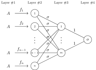
Figure 1: Visualization of our neural network in Section 4. Here $m=O(\log n)$.

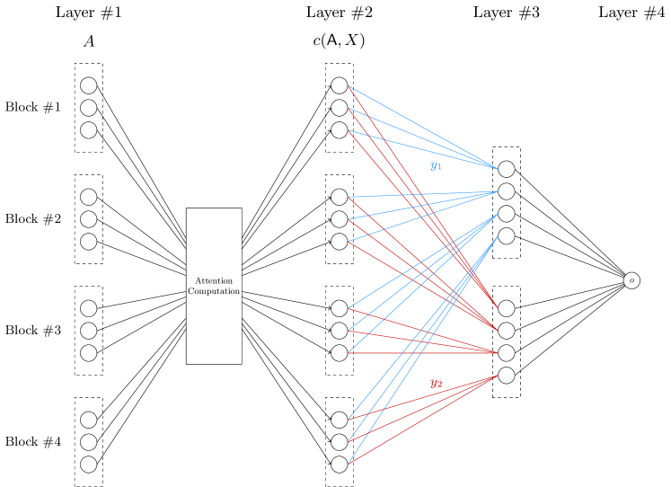
Figure 2: This is structure for self-attention. Let $A=A_{1}=A_{2}=A_{3}\in\mathbb{R}^{n\times d}$. Let $\mathsf{A}=A_{1}\otimes A_{2}$. Let $n=4$, $d=3$, $m=2$. Let $y_{1}\in\mathbb{R}^{d}$. Let $c(\operatorname{\mathsf{A}},x)\in\mathbb{R}^{n\times d}$ which is $\mathbb{R}^{4\times 3}$. Let $c(\operatorname{\mathsf{A}},x)_{1}\in\mathbb{R}^{3}$ denote the first block in layer 2. For the first node in first block in layer 3, the computation is based on ReLU of $\langle c(\operatorname{\mathsf{A}},X)_{1},y_{1}\rangle$.

Definition 3.6.

We define a four-layer neural network(with linear attention and ReLU activation) $F_{\operatorname{lin}}:\mathbb{R}^{n\times d}\rightarrow\mathbb{R}$ $F_{\exp}(A;x,y):=\phi(\sum_{j=1}^{m}\phi_{\tau}(\langle f_{\operatorname{lin}}(A,x),y_{j}\rangle))$

Definition 3.7.

Let $C>1$ denote some constant. Let $m=C\log(n/\delta)$. Let $y\in\mathbb{R}^{n\times m}$, for each $j\in[m]$, we use $y_{j}$ to denote the $j$-th column of $y$. For each entry in $y_{j}$ we sampled it from Rademacher random variable distribution.

The settings of the above neural network are natural in deep learning theory [96, 54, 35, 7, 8, 71, 74, 15, 3, 63].

3.3 Definition of Datasets for Binary Classification

Definition 3.8 (Binary classification).

Given two sets of datasets ${\cal D}_{0}$ and ${\cal D}_{1}$.

• For each $A\in\mathbb{R}^{n\times d}$ from ${\cal D}_{0}$, we assume that $(Ax)_{i}\in[\log n,1.4\log n]$ for all $i\in[n]$

• For each $A\in\mathbb{R}^{n\times d}$ from ${\cal D}_{1}$, we assume that there is one index $j\in[n]$ such that $(Ax)_{j}=4\log n$ and for all $i\in[n]\backslash\{j\}$, we have $(Ax)_{i}\in[\log n,1.4\log n]$

4 Property of Dataset

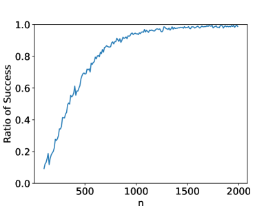
(a) Ratio of Success with respect to $n$

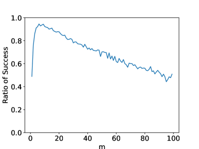
(b) Ratio of Success with respect to $m$

Figure 3: Figure for the softmax regression model

Lemma 4.1.

Let $\sigma\sim\{-1,+1\}^{n}$ denote a random sign vector. Let $C>1$ be a sufficiently large constant. Let $\delta\in(0,0.1)$. Then, for each $A\in{\cal D}_{0}$, we have Part 1. $~{}\Pr_{\sigma}[|\sum_{i=1}^{n}f_{\operatorname{lin}}(A,x)_{i}\sigma_{i}|\leq C\frac{\sqrt{\log(n/\delta)}}{\sqrt{n}}]\geq~{}1-\delta/\operatorname{poly}(n)$ Part 2. $~{}\Pr_{\sigma}[|\sum_{i=1}^{n}f_{\exp}(A,x)_{i}\sigma_{i}|\leq C\frac{\sqrt{\log(n/\delta)}}{n^{0.1}}]\geq~{}1-\delta/\operatorname{poly}(n)$

Proof.

Proof of Part 1. Note that we can show that

$$|f_{\operatorname{lin}}(A,x)_{i}|= ~{}\alpha_{\operatorname{lin}}(A,x)^{-1}|u_{\operatorname{lin}}(A,x)_{i}|$$

$$\leq ~{}(n\log n)^{-1}\cdot(1.4\log n)$$

$$\leq ~{}\frac{2}{n}$$

where the first step follows from the definition of $\alpha$, the second step follows from Definition 3.8 and the last step follows from simple algebra.

Thus, applying Hoeffding inequality, we can get with probability $1-\delta/\operatorname{poly}(n)$,

$$|\sum_{i=1}^{n}f_{\operatorname{lin}}(A,x)_{i}\sigma_{i}|\leq~{}C\frac{\sqrt{n\log(n/\delta)}}{n}=~{}C\frac{\sqrt{\log(n/\delta)}}{\sqrt{n}}$$

Proof of Part 2. For all $i\in[n]$, we know that

$$|f_{\exp}(A,x)_{i}|= ~{}\alpha_{\exp}(A,x)^{-1}\cdot|u_{\exp}(A,x)_{i}|$$

$$\leq ~{}(n\cdot n)^{-1}\cdot(n^{1.4})$$

$$= ~{}\frac{1}{n^{0.6}}$$

Thus, applying Hoeffding inequality, we can get with probability $1-\delta/\operatorname{poly}(n)$,

$$|\sum_{i=1}^{n}f_{\exp}(A,x)_{i}\sigma_{i}|\leq ~{}C\frac{\sqrt{n\log(n/\delta)}}{n^{0.6}}$$

$$\leq ~{}C\frac{\sqrt{\log(n/\delta)}}{n^{0.1}}$$

∎

Lemma 4.2.

Let $\sigma\sim\{-1,+1\}^{n}$ denote a random sign vector. Let $C>1$ be a sufficiently large constant. Let $\delta\in(0,0.1)$. Then, for each $A\in{\cal D}_{1}$, we have

• Part 1. $\Pr_{\sigma}[|\sum_{i=1}^{n}f_{\operatorname{lin}}(A,x)_{i}\sigma_{i}|\leq C\sqrt{\log(n/\delta)/n}]\geq 1-\delta/\operatorname{poly}(n)$

• Part 2. $\Pr_{\sigma}[|\sum_{i=1}^{n}f_{\exp}(A,x)_{i}\sigma_{i}|\geq 1/4]\geq 1$

• Part 3. $\Pr[\sum_{i=1}^{n}f_{\exp}(A,x)_{i}\sigma_{i}>0]=1/2$ and $\Pr[\sum_{i=1}^{n}f_{\exp}(A,x)_{i}\sigma_{i}<0]=1/2$

Proof.

Proof of Part 1. we can show that

$$|f_{\operatorname{lin}}(A,x)_{i}|= ~{}\alpha_{\operatorname{lin}}(A,x)^{-1}|u(A,x)_{i}|$$

$$\leq ~{}((n-1)\log n+4\log n)^{-1}\cdot(4\log n)$$

$$= ~{}\frac{4}{n+3}$$

$$\leq ~{}\frac{4}{n}$$

where the first step follows from the definition of $f_{\operatorname{lin}}$, the second step follows from Definition 3.8, the third step follows from simple algebra and the last step follows from simple algebra.

Applying Hoeffding inequality again, we finish the proof.

Proof of Part 2.

There is one index $j\in[n]$, we know that

$$|f_{\exp}(A,x)_{j}|= ~{}\alpha_{\exp}(A,x)^{-1}\cdot|u_{\exp}(A,x)_{j}|$$

$$\geq ~{}(n^{1.4}\cdot(n-1)+n^{4})^{-1}\cdot(n^{4})$$

$$\geq ~{}\frac{1}{2}$$

For all the $i\in[n]\backslash\{j\}$, we know that

$$|f_{\exp}(A,x)_{i}|= ~{}\alpha_{\exp}(A,x)^{-1}\cdot|u_{\exp}(A,x)_{i}|$$

$$\leq ~{}(n\cdot(n-1)+n^{4})^{-1}\cdot(n^{1.4})$$

$$\leq ~{}\frac{1}{n^{2.6}}$$

Thus, it is obvious that

$$|\sum_{i=1}^{n}f_{\exp}(A,x)_{i}\sigma_{i}|\geq\frac{1}{2}-(n-1)\cdot\frac{1}{n^{2.6}}\geq 1/4$$

where the last step follows from $n\geq 4$.

Proof of Part 3. The sign is completely decided by $\sigma_{j}$, thus it has $1/2$ chance to be positive and $1/2$ chance to be negative. ∎

5 Binary Classification

In this section, we provide an overview of theoretical analysis of the performance of different models in binary classification task.

5.1 Softmax Attention

Lemma 5.1.

For each data $A$ from ${\cal D}_{0}$, $F_{\exp}(A)=0$ with probability at least $1-\delta/\operatorname{poly}(n)$.

Proof.

Note that all the $y_{l}$ are independent, for each $l\in[m]$, we call Part 2 of Lemma 4.1, we can show that $\phi_{\tau}(\langle f_{\exp}(A,x),y_{l}\rangle)=0$.

Since $m\leq\delta/\operatorname{poly}(n)$, we are allowed to take union bound over all $l\in[m]$. Thus, we have $F_{\operatorname{lin}}(A,x)=\phi(\sum_{l=0}^{m}\phi_{\tau}(\langle f_{\exp}(A,x),y_{l}\rangle))=0.$ ∎

Lemma 5.2.

For each data $A$ from ${\cal D}_{1}$, $F_{\exp}(A)>0$ with probability at least $1-\delta/\operatorname{poly}(n)$.

Proof.

By Part 2 and 3 of Lemma 4.2, we have $\phi_{\tau}(\langle f_{\exp}(A,x),y_{l}\rangle)>1/4$ with probability $1/2$.

Since all $l\in[m]$ are independent, thus there exists one $l\in[m]$ such that

$$\phi_{\tau}(\langle f_{\exp}(A,x),y_{l}\rangle)>1/4$$

the probability is $1-(1/2)^{m}\geq 1-\delta/\operatorname{poly}(n)$.

Thus, with probability $1-\delta/\operatorname{poly}(n)$, we have

$$F_{\exp}(A,x)=\phi(\sum_{l=0}^{m}\phi_{\tau}(\langle f_{\exp}(A,x),y_{l}\rangle))>0$$

holds. ∎

5.2 Linear Attention

Lemma 5.3.

For each data $A$ from ${\cal D}_{0}$, $F_{\operatorname{lin}}(A)=0$ with probability at least $1-\delta/\operatorname{poly}(n)$.

Proof.

Note that all the $y_{l}$ are independent, for each $l\in[m]$, we call Part 1 of Lemma 4.1, we can show that $\phi_{\tau}(\langle f_{\operatorname{lin}}(A,x),y_{l}\rangle)=0$.

Since $m\leq\delta/\operatorname{poly}(n)$, we are allowed to take union bound over all $l\in[m]$. Thus, we have $F_{\operatorname{lin}}(A,x)=\phi(\sum_{l=0}^{m}\phi_{\tau}(\langle f_{\operatorname{lin}}(A,x),y_{l}\rangle))=0$. ∎

Lemma 5.4.

For each data $A$ from ${\cal D}_{1}$, $F_{\operatorname{lin}}(A)=0$ with probability at least $1-\delta/\operatorname{poly}(n)$.

Proof.

Note that all the $y_{l}$ are independent, for each $l\in[m]$, we call Part 1 of Lemma 4.2, we can show that $\phi_{\tau}(\langle f_{\operatorname{lin}}(A,x),y_{l}\rangle)=0$.

Since $m\leq\delta/\operatorname{poly}(n)$, we are allowed to take union bound over all $l\in[m]$.

Thus, we have $F_{\operatorname{lin}}(A,x)=\phi(\sum_{l=0}^{m}\phi_{\tau}(\langle f_{\operatorname{lin}}(A,x),y_{l}\rangle))=0$ ∎

6 Main Results

We provide more details for self-attention result, for details of cross-attention, we refer the readers to appendix.

Definition 6.1 (Self-Attention dataset distribution, informal version of Definition D.1).

We define $a_{0}\in(0,0.1)$. We denote $a_{1}\geq 0.7$. Let $b+c=1$ for $b\geq 0.1,c\geq 0.1$. Assume $n=(d-2)t$ where $t$ is a positive integer.

Given two sets of datasets ${\cal D}_{0}$ and ${\cal D}_{1}$. For each $A_{1}\in{\cal D}_{0}$, we have the first column of $A_{1}$ is $e_{j_{3}}\cdot a_{0}\sqrt{\log n}$ for some $j_{3}\in[n]$. From the second column to the $(d-1)$-th columns of $A_{1}$ are $\begin{bmatrix}I_{d-2}\\ I_{d-2}\\ \vdots\\ I_{d-2}\end{bmatrix}\cdot b\sqrt{\log n}$. The last column of $A_{1}$ is ${\bf 1}_{n}\cdot c\sqrt{\log n}$.

Assume $n=(d-2)t$ where $t$ is a positive integer. For each $A_{1}\in{\cal D}_{1}$, we have Type I column: the first column of $A_{1}$ is $e_{j_{3}}\cdot a_{1}\sqrt{\log n}$ for $j_{3}\in[n]$. Type II column: from the second column to the $(d-1)$-th columns of $A_{1}$ are $\begin{bmatrix}I_{d-2}\\ I_{d-2}\\ \vdots\\ I_{d-2}\end{bmatrix}\cdot b\sqrt{\log n}$. Type III column: the last column of $A_{1}$ is ${\bf 1}_{n}\cdot c\sqrt{\log n}$.

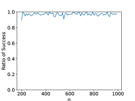
(a) Vary with $n$

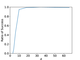
(b) Var with $d$

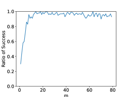
(c) Vary with $m$

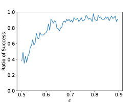
(d) Vary with $c$

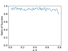
(e) Vary with $a_{0}$

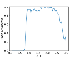
(f) Vary with $a_{1}$

Figure 4: Self-Attention when $X=\mathrm{vec}(I_{d})$. Let $n$ denote the length of input sentence. Let $d$ denote the embedding size. Let $m$ denotes the width of the second layer. Let $a_{1},a_{0},c$ denote the parameters of dataset ${\cal D}_{0}$ and ${\cal D}_{1}$.

(a) Vary with $n$

(b) Vary with $d$

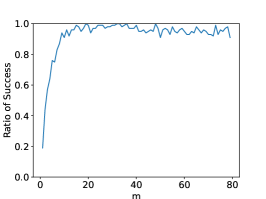
(c) Vary with $m$

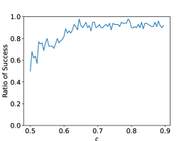
(d) Vary with $c$

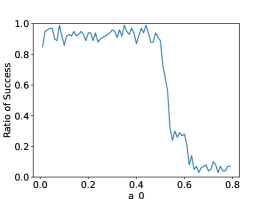
(e) Vary with $a_{0}$

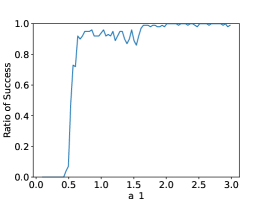
(f) Vary with $a_{1}$

Figure 5: Self-Attention when $X=\mathbf{1}_{n^{2}}$. Let $n$ denote the length of input sentence. Let $d$ denote the embedding size. Let $m$ denotes the width of the second layer. Let $a_{1},a_{0},c$ denote the parameters of dataset ${\cal D}_{0}$ and ${\cal D}_{1}$.

Theorem 6.2 (Main results, informal version of Section D).

Let $\tau=(c+0.1)\sqrt{\log n}$ Let $d\in[\omega(n^{0.02}),n]$ Let $m=O(\log(n/\delta))$ Let $x={\bf 1}_{d^{2}}$ Let

$$F_{\exp}(A_{1}):=\phi(\sum_{j_{0}=1}^{n}\sum_{l=1}^{m}\phi_{\tau}(\langle\mathsf{Att}_{j_{0},*},y_{l}\rangle))$$

where $\mathsf{Att}_{j_{0},*}$ denote the $j_{0}$-th line of Eq. (1). For any $A_{1}$ from ${\cal D}_{1}$ (Definition D.1) With high probability $1-\delta/\operatorname{poly}(n)$, we have

$$F_{\exp}(A_{1})>0,~{}F_{\exp}(A_{1})=0$$

For any $A_{1}$ from ${\cal D}_{0}$ (Definition D.1) With high probability $1-\delta/\operatorname{poly}(n)$, we have

$$F_{\operatorname{lin}}(A_{1})=0,~{}F_{\operatorname{lin}}(A_{1})=0$$

7 Numerical Experiments

Here in this section, we present our numerical experiments of our proof. We ran simulation experiments on the softmax regression model, the self attention model and the cross attention model. We deploy all our experiments on an Apple MacBook Pro with M2 chip and 16GB of memory. The Python we use is version 3.9.12.

7.1 Softmax Regression Model

We set the dataset as described in Section 4. For a pair of inputs $(A_{0},x_{0})\in\mathcal{D}_{0}$ and $(A_{1},x_{1})\in\mathcal{D}_{1}$, we define the event $E_{\mathrm{success}}$ as

$$E_{\mathrm{success}}:= ~{}F_{\exp}(A_{1},x_{1})>0\land~{}F_{\operatorname{lin}}(A_{1},x_{1})=0$$

$$\land ~{}F_{\exp}(A_{0},x_{0})=0\land~{}F_{\operatorname{lin}}(A_{0},x_{0})=0.$$

We divide our numerical experiments for parameters $n$ and $m$. To be specific,

• We deploy experiments for $n\in[100,2000]$ with a step size of $10$. For each $n$, we set $m=\log n$. For each group of the parameters, we generated the models for $1000$ times and count the times $E_{\mathrm{success}}$ happens. The result can be found in Figure (a) in Figure 3.

• We fix $n=1000$, and deploy experiments for $m\in[1,100]$ with a step size of $1$. For each group of the parameters, we generated the models for $1000$ times and count the counts $E_{\mathrm{success}}$ happens. The result can be found in Figure (b) in Figure 3.

7.2 Experiments for Self-Attention

We set the dataset as described in Section D.1. For a pair of inputs $(A_{01},A_{02},A_{03})\in\mathcal{D}_{0}$ and $(A_{11},A_{12},A_{13})\in\mathcal{D}_{1}$, we define the event $E_{\mathrm{success}}$ as

$$E_{\mathrm{success}}:= ~{}F_{\exp}(A_{11},A_{12},A_{13})>0$$

$$\land ~{}F_{\operatorname{lin}}(A_{11},A_{12},A_{13})=0$$

$$\land ~{}F_{\exp}(A_{01},A_{02},A_{03})=0$$

$$\land ~{}F_{\operatorname{lin}}(A_{01},A_{02},A_{03})=0.$$

7.2.1 For $X=\mathrm{vec}(I_{d})$

We first fix $X=\mathrm{vec}(I_{d})$, and deploy the numerical experiments for parameters $n$, $d$, $m$, $c$, $a_{0}$ and $a_{1}$. To be specific,

• We deploy experiments for $n\in[200,1000]$ with a step size of $10$. For each $n$, we set $d=12$, $\delta=0.01$, $m=\max\{\log(n/\delta),15\}$, $a_{0}=0.01$, $a_{1}=1.2$, $b=0.2$, $c=0.8$. For each set of parameters, we iteratively generated models 100 times and recorded the occurrences of successful events denoted as $E_{\mathrm{success}}$. The result can be found in Figure (a) in Figure 4.

• We deploy experiments for $d\in\{4,6,10,18,34,66\}$. For each $d$, we set $n=256$, $\delta=0.01$, $m=\max\{\log(n/\delta),15\}$, $a_{0}=0.01$, $a_{1}=1.2$, $b=0.2$, $c=0.8$. For each set of parameters, we iteratively generated models 100 times and recorded the occurrences of successful events denoted as $E_{\mathrm{success}}$. The result can be found in Figure (b) in Figure 4.

• We deploy experiments for $m\in[1,80]$ with a step size of $1$. For each $m$, we set $n=200$, $d=22$, $\delta=0.01$, $a_{0}=0.01$, $a_{1}=1.2$, $b=0.2$, $c=0.8$. For each set of parameters, we iteratively generated models 100 times and recorded the occurrences of successful events denoted as $E_{\mathrm{success}}$. The result can be found in Figure (c) in Figure 4.

• We deploy experiments for $a_{1}\in[0.1,3]$ with a step size of $0.036$. For each $a_{1}$, we set $n=200$, $d=22$, $\delta=0.01$, $m=\max\{\log(n/\delta),15\}$, $a_{0}=0.01$, $b=0.2$, $c=0.8$. For each set of parameters, we iteratively generated models 100 times and recorded the occurrences of successful events denoted as $E_{\mathrm{success}}$. The result can be found in Figure (d) in Figure 4.

• We deploy experiments for $a_{0}\in[0.01,0.8]$ with a step size of $0.01$. For each $a_{0}$, we set $n=200$, $d=22$, $\delta=0.01$, $m=\max\{\log(n/\delta),15\}$, $a_{0}=0.01$, $a_{1}=1.2$, $b=0.2$, $c=0.8$. For each set of parameters, we iteratively generated models 100 times and recorded the occurrences of successful events denoted as $E_{\mathrm{success}}$. The result can be found in Figure (e) in Figure 4.

• We deploy experiments for $c\in[0.5,0.9]$ with a step size of $0.005$. For each $c$, we set $n=200$, $d=22$, $\delta=0.01$, $m=\max\{\log(n/\delta),15\}$, $a_{1}=1.2$, $b=0.2$. For each set of parameters, we iteratively generated models 100 times and recorded the occurrences of successful events denoted as $E_{\mathrm{success}}$. The result can be found in Figure (f) in Figure 4.

7.2.2 For $X=\mathbf{1}_{n^{2}}$

For the setting that $X=\mathbf{1}_{n^{2}}$, we similarly deploy the experiments on parameters $n$, $d$, $m$, $c$, $a_{0}$ and $a_{1}$. The parameter setting and choice are the same as above. The experiment result is shown in Figure 5.

8 Conclusion

The transformer architecture, propelled by its attention mechanism, has revolutionized natural language processing tasks. Particularly, the softmax function utilized in the attention mechanism plays a crucial role in grasping the token interactions within sequences. On the flip side, linear attention, while computationally more efficient, falls short in its performance compared to softmax attention. This paper delves into the core reasons for this observed discrepancy. Through meticulous comparative analysis, it has been elucidated that softmax-based neural networks are more adept at distinguishing between certain datasets compared to their linear attention counterparts, both in self-attention and cross-attention scenarios. This pivotal revelation offers profound insights into the intrinsic workings of attention mechanisms, thereby guiding the path for more optimized future model developments.

Appendix

Roadmap. We organize the appendix as follows. Section A provides some preliminaries. We discuss more related work in Section B. Section C describes the attention model setting. Section D gives analysis for self attention when $QK^{\top}=\mathbf{1}^{d\times d}$ while Section E gives a further discussion when $QK^{\top}=I_{d}$. Section F provides analysis for cross attention model, with the result figure of our experiment.

Appendix A Preliminary

Notations. We used $\mathbb{R}$ to denote real numbers. We use $A\in\mathbb{R}^{n\times d}$ to denote an $n\times d$ size matrix where each entry is a real number. We use $e_{j}$ to denote the unit vector where $j$-th entry is $1$ and others are $0$. For any positive integer $n$, we use $[n]$ to denote $\{1,2,\cdots,n\}$. For a matrix $A\in\mathbb{R}^{n\times d}$, we use $a_{i,j}$ to denote the an entry of $A$ which is in $i$-th row and $j$-th column of $A$, for each $i\in[n]$, $j\in[d]$. For two vectors $a,b$, we use $\langle a,b\rangle$ to denote their inner product. We use ${\bf 1}_{n}$ to denote a length-$n$ vector where all the entries are ones, and use ${\bf 1}_{n\times n}$ to denote a $n\times n$ matrix where all the entries are ones. For a vector $x$ or a matrix $A$, we use $\exp(x)$ and $\exp(A)$ to denote the entry-wise exponential operation on them. For matrices $A\in\mathbb{R}^{n_{1}\times d_{1}}$ and $B\in\mathbb{R}^{n_{2}\times d_{2}}$, we use $A\otimes B\in\mathbb{R}^{n_{1}n_{2}\times d_{1}d_{2}}$ to denote a matrix such that its $((i_{1}-1)n_{2}+i_{2},(j_{1}-i)d_{2}+j_{2})$-th entry is $A_{i_{1},j_{1}}\cdot B_{i_{2},j_{2}}$ for all $i_{1}\in[n_{1}],j_{1}\in[d_{1}],i_{2}\in[n_{2}],j_{2}\in[d_{2}]$. For a matrix $A\in\mathbb{R}^{n\times d}$, we use $\mathrm{vec}(A)\in\mathbb{R}^{nd}$ to denote the vectorization of $A$. We use $I_{d}$ to denote the $d\times d$ identity matrix. We use $A^{\top}$ to denote the transpose of a matrix $A$.

Using standard tensor-trick [40, 41, 39, 4, 5], we know that

Fact A.1 (Tensor-trick).

Let $A_{1},A_{2}\in\mathbb{R}^{n\times d}$, let $Q\in\mathbb{R}^{d\times d}$, let $K\in\mathbb{R}^{d\times d}$, we have

$$\operatorname{vec}(\exp(A_{1}QK^{\top}A_{2}^{\top}))=\exp(\operatorname{\mathsf{A}}\operatorname{vec}(QK^{\top}))$$

where $\operatorname{\mathsf{A}}:=A_{1}\otimes A_{2}\in\mathbb{R}^{n^{2}\times d^{2}}$.

Appendix B More Related Works

Theory of Transformer.

With the ascent of LLMs, there’s a heightened interest in comprehending their learning prowess and deepening the theoretical underpinnings of transformer models. A key focus is the in-context learning ability of transformers. [43] empirically demonstrated that transformers can adeptly learn linear function classes in-context. [6] linked in-context learning in transformers to conventional learning algorithms, a connection further validated through linear regression. [91] explored the in-context learning of a single-head self-attention layer, noting its strengths and weaknesses. [85] viewed LLMs through a Bayesian lens, interpreting in-context learning as a Bayesian selection process. Delving into the transformer’s architecture, [67] introduced the ”skill location” concept, emphasizing how minor parameter tweaks during fine-tuning can drastically impact performance and continual learning. On the capabilities front, [70] analyzed the strengths and limitations of transformers, highlighting their varying growth rates in different tasks. [10] provided an in-depth analysis of GPT-4 [64], lauding its versatility across domains and advocating for more advanced models. Our research now pivots to a unique 2-layer regression problem, inspired by the transformer paradigm.

Boosting Computation of Attention.

The task of fine-tuning pre-trained LLMs presents challenges, primarily due to their extensive parameter sets. Efforts have been directed towards devising efficient methods for computing the attention module. The use of locality sensitive hashing (LSH) for attention approximation has been a topic of discussion in several studies, as seen in [49] and [24]. Specifically, [49] introduced two methods to enhance computational efficiency. They employed LSH as an alternative to dot product attention, resulting in a notable reduction in time complexity. Additionally, they adopted a reversible residual layer in place of the conventional residual layer. On the other hand, [24] refined the approximation technique, noting that LSH doesn’t consistently demand updates to model parameters. In a different approach, [66] proposed approximation methods that leverage a transformer-in-transformer (TinT) model to emulate both the forward pass and back-propagation of a transformer, leading to enhanced parameter efficiency. [62] delved into the efficient fine-tuning of LLMs, especially those with substantial memory requirements. Building upon the traditional ZO-SCD optimizer, they crafted the memory-efficient MeZO gradient estimator that operates using only the forward pass. Furthermore, [4] established a stringent bound for static attention, while [16] validated results concerning the dynamic attention issue. Lastly, [42] unveiled a quantum algorithm tailored for attention computation.

Optimizer for LLMs.

Gradient-based algorithms remain a cornerstone in machine learning. In recent times, there has been a surge in research efforts aimed at devising efficient optimizers tailored for LLM-centric optimization challenges. [23] explored large-scale optimization scenarios where basic vector operations on decision variables become unfeasible. To address this, they employed a block gradient estimator, formulating an algorithm that markedly cuts down both query and computational complexities per iteration. Taking a different approach, [69] introduced the Direct Preference Optimization algorithm. This method fine-tunes LLMs directly using a specified human preference dataset, bypassing the need for explicit reward models or reinforcement learning techniques. In another significant contribution, [55] unveiled an adept second-order optimizer for LLMs. This optimizer is grounded in diagonal Hessian approximation coupled with a clipping mechanism. Interestingly, they also eased the stipulation that the Hessian must be Lipschitz continuous in their convergence proof. Drawing inspiration from this innovative perspective, our research employs a congruent proof methodology, especially when addressing the ReLU function within our regression analysis.

Appendix C Analysis for $Q,K,V$ Attention

In Section C.1, we give the definition of linear attention. In Section C.2, we give the definition of softmax attention.

C.1 Linear Attention

Definition C.1 (Linear Attention).

Given $A_{1},A_{2},A_{3}\in\mathbb{R}^{n\times d}$.

Let $x=\operatorname{vec}(QK^{\top})\in\mathbb{R}^{d^{2}}$. Let $\operatorname{\mathsf{A}}=A_{1}\otimes A_{2}\in\mathbb{R}^{n^{2}\times d^{2}}$.

Let $V\in\mathbb{R}^{d\times d}$.

Let $\operatorname{\mathsf{A}}_{j_{0}}\in\mathbb{R}^{n\times d^{2}}$ denote the $j_{0}$-th block of $\operatorname{\mathsf{A}}$.

For each $j_{0}\in[n]$, we define $u_{\operatorname{lin}}(\operatorname{\mathsf{A}},x)_{j_{0}}\in\mathbb{R}^{n}$ as follows

$$u_{\operatorname{lin}}(\operatorname{\mathsf{A}},x)_{j_{0}}:=\operatorname{\mathsf{A}}_{j_{0}}x$$

We define $\alpha_{\operatorname{lin}}(\operatorname{\mathsf{A}},x)_{j_{0}}$ as follows

$$\alpha_{\operatorname{lin}}(\operatorname{\mathsf{A}},x)_{j_{0}}:=\langle u_{\operatorname{lin}}(\operatorname{\mathsf{A}},x)_{j_{0}},{\bf 1}_{n}\rangle$$

We define $f_{\operatorname{lin}}(\operatorname{\mathsf{A}},x)_{j_{0}}$ as follows

$$f_{\operatorname{lin}}(\operatorname{\mathsf{A}},x)_{j_{0}}=\alpha_{\operatorname{lin}}(\operatorname{\mathsf{A}},x)_{j_{0}}^{-1}\cdot u_{\operatorname{lin}}(\operatorname{\mathsf{A}},x)_{j_{0}}$$

We define $c_{\operatorname{lin}}(\operatorname{\mathsf{A}},x)_{j_{0}}\in\mathbb{R}^{d}$ as follows

$$c_{\operatorname{lin}}(\operatorname{\mathsf{A}},x)_{j_{0},i_{0}}:=\langle\underbrace{f_{\operatorname{lin}}(\operatorname{\mathsf{A}},x)_{j_{0}}}_{n\times 1},\underbrace{(A_{3}V)_{i_{0}}}_{n\times 1}\rangle,~{}~{}~{}\forall i_{0}\in[d]$$

Definition C.2.

Let $y\in\mathbb{R}^{d\times m}$. Let $y_{l}\in\mathbb{R}^{d}$ denote the $l$-th column of $y$. We define

$$F_{\operatorname{lin}}(A_{1},A_{2},A_{3}):=\phi(\sum_{j_{0}=1}^{n}\sum_{l=1}^{m}\phi_{\tau}(\langle\underbrace{c_{\operatorname{lin}}(\operatorname{\mathsf{A}},x)_{j_{0}}}_{d\times 1},\underbrace{y_{l}}_{d\times 1}\rangle))$$

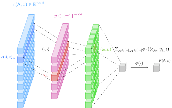
Figure 6: Visualization of our attention computation.

Claim C.3 (Equivalence Formula).

If the following conditions hold,

• Let $x=\operatorname{vec}(QK^{\top})$

• Let $(A_{1})_{j_{0},*}$ denote the $j_{0}$-th row of $A_{1}\in\mathbb{R}^{n\times d}$

• Let $\operatorname{\mathsf{A}}=A_{1}\otimes A_{2}$

Then, we have

• $u_{\operatorname{lin}}(\operatorname{\mathsf{A}},x)_{j_{0}}=((A_{1})_{j_{0},*}QK^{\top}A_{2}^{\top})^{\top}$

• $\alpha_{\operatorname{lin}}(A,x)_{j_{0}}=\langle((A_{1})_{j_{0},*}QK^{\top}A_{2}^{\top})^{\top},{\bf 1}_{n}\rangle$

Proof.

The proofs are directly following from tensor-trick (Fact A.1). ∎

C.2 Softmax Attention

Definition C.4 (Softmax Attention).

Given $A_{1},A_{2},A_{3}\in\mathbb{R}^{n\times d}$.

Let $x=\operatorname{vec}(QK^{\top})\in\mathbb{R}^{d^{2}}$. Let $\operatorname{\mathsf{A}}=A_{1}\otimes A_{2}\in\mathbb{R}^{n^{2}\times d^{2}}$.

Let $\operatorname{\mathsf{A}}_{j_{0}}\in\mathbb{R}^{n\times d^{2}}$ denote the $j_{0}$-th block of $\operatorname{\mathsf{A}}$.

For each $j_{0}\in[n]$, we define $u_{\exp}(\operatorname{\mathsf{A}},x)_{j_{0}}\in\mathbb{R}^{n}$ as follows

$$u_{\exp}(\operatorname{\mathsf{A}},x)_{j_{0}}:=\exp(\operatorname{\mathsf{A}}_{j_{0}}x)$$

We define $\alpha_{\exp}(\operatorname{\mathsf{A}},x)_{j_{0}}$ as follows

$$\alpha_{\exp}(\operatorname{\mathsf{A}},x)_{j_{0}}:=\langle u_{\exp}(\operatorname{\mathsf{A}},x)_{j_{0}},{\bf 1}_{n}\rangle$$

We define $f_{\exp}(\operatorname{\mathsf{A}},x)_{j_{0}}$ as follows

$$f_{\exp}(\operatorname{\mathsf{A}},x)_{j_{0}}=\alpha_{\exp}(\operatorname{\mathsf{A}},x)_{j_{0}}^{-1}\cdot u_{\exp}(\operatorname{\mathsf{A}},x)_{j_{0}}$$

We define $c_{\exp}(\operatorname{\mathsf{A}},x)_{j_{0}}\in\mathbb{R}^{d}$ as follows

$$c_{\exp}(\operatorname{\mathsf{A}},x)_{j_{0},i_{0}}:=\langle f_{\exp}(\operatorname{\mathsf{A}},x)_{j_{0}},(A_{3}V)_{i_{0}}\rangle,~{}~{}~{}\forall i_{0}\in[d]$$

Claim C.5 (Equivalence Formula).

If the following conditions hold,

• Let $x=\operatorname{vec}(QK^{\top})$

• Let $(A_{1})_{j_{0},*}$ denote the $j_{0}$-th row of $A_{1}\in\mathbb{R}^{n\times d}$

• Let $\operatorname{\mathsf{A}}=A_{1}\otimes A_{2}$

Then, we have

• $u_{\exp}(\operatorname{\mathsf{A}},x)_{j_{0}}=(\exp((A_{1})_{j_{0},*}QK^{\top}A_{2}^{\top}))^{\top}$

• $\alpha_{\exp}(A,x)_{j_{0}}=\langle(\exp((A_{1})_{j_{0},*}QK^{\top}A_{2})^{\top})^{\top},{\bf 1}_{n}\rangle$

Proof.

The proofs are directly following from tensor-trick (Fact A.1). ∎

Definition C.6.

Let $y\in\mathbb{R}^{n\times m}$. Let $y_{l}\in\mathbb{R}^{n}$ denote the $l$-th column of $y$. We define

$$F_{\exp}(A_{1},A_{2},A_{3}):=\phi(\sum_{j_{0}=1}^{n}\sum_{l=1}^{m}\phi_{\tau}(\langle c_{\exp}(\operatorname{\mathsf{A}},x)_{j_{0}},y_{l}\rangle))$$

Appendix D Self-Attention Dataset

In Section D.1, we give the definition of the dataset used in the following sections for self-attention. In Section D.2, we show that the output of the $F_{\exp}$ is greater than $0$ with high probability. In Section D.3, we show that the output of $F_{\exp}$ is equal to $0$ with high probability. In Section D.4, we show that the output of the $F_{\operatorname{lin}}$ is equal to $0$ with high probability. In Section D.5, we show that the output of $F_{\operatorname{lin}}$ is equal to $0$ with high probability.

D.1 Definition of Dataset

Definition D.1 (Self-Attention dataset distribution).

We define

• $a_{0}\in(0,0.1)$

• Let $a_{1}\geq 0.7$

• $b+c=1$ for $b\geq 0.1,c\geq 0.1$

Given two sets of datasets ${\cal D}_{0}$ and ${\cal D}_{1}$

• For each $\{A_{1},A_{2},A_{3}\}\in{\cal D}_{0}$, we have

  • $A_{1}=A_{2}=A_{3}\in\mathbb{R}^{n\times d}$

  • Assume $n=(d-2)t$ where $t$ is a positive integer

  • the first column of $A_{1}$ is $e_{j_{3}}\cdot a_{0}\sqrt{\log n}$ for some $j_{3}\in[n]$

  • from the second column to the $(d-1)$-th columns of $A_{1}$ are $\begin{bmatrix}I_{d-2}\\ I_{d-2}\\ \vdots\\ I_{d-2}\end{bmatrix}\cdot b\sqrt{\log n}$

  • the last column of $A_{1}$ is ${\bf 1}_{n}\cdot c\sqrt{\log n}$

• For each $\{A_{1},A_{2},A_{3}\}\in{\cal D}_{1}$, we have

  • $A_{1}=A_{2}=A_{3}\in\mathbb{R}^{n\times d}$

  • Assume $n=(d-2)t$ where $t$ is a positive integer

  • Type I column: the first column of $A_{1}$ is $e_{j_{3}}\cdot a_{1}\sqrt{\log n}$ for $j_{3}\in[n]$

  • Type II column: from the second column to the $(d-1)$-th columns of $A_{1}$ are $\begin{bmatrix}I_{d-2}\\ I_{d-2}\\ \vdots\\ I_{d-2}\end{bmatrix}\cdot b\sqrt{\log n}$

  • Type III column: the last column of $A_{1}$ is ${\bf 1}_{n}\cdot c\sqrt{\log n}$

D.2 Dataset 1 with $F_{\exp}$

In Section D.2.1 we analyse the property of dataset 1 with respect to function $u_{\exp}$ and $f_{\exp}$. In Section D.2.2 we analyse the property of dataset 1 with respect to function $c_{\exp}$. In Section D.2.3 we analyse the property of dataset 1 with respect to function $c_{\exp}$ with random signs. In Section D.2.4 we show the property of dataset 1 with respect to the output of $F_{\exp}$.

D.2.1 Dataset 1 Property when applying function $u_{\exp}$ and $f_{\exp}$

Lemma D.2.

If the following conditions hold

• Let $b+c=1$

• Let $\{A_{1},A_{2},A_{3}\}$ from dataset ${\cal D}_{1}$ (see Definition D.1)

• Let $QK^{\top}={\bf 1}_{d\times d}$ (This is the major difference compared to Lemma E.1)

Then, for $u_{\exp}(\operatorname{\mathsf{A}},x)_{j_{0},j_{1}}$ and $f_{\exp}(\operatorname{\mathsf{A}},x)_{j_{0},j_{1}}$ entry we have

• Part 1. For $j_{0}=j_{3}$,

  • Part 1a. For $j_{1}=j_{3}$, then $u_{\exp}(\operatorname{\mathsf{A}},x)_{j_{0},j_{1}}=n^{(1+a_{1})^{2}}$.

  • Part 1b. For $j_{1}\neq j_{3}$, then $u_{\exp}(\operatorname{\mathsf{A}},x)_{j_{0},j_{1}}=n^{1+a_{1}}$.

• Part 2. For $j_{0}\neq j_{3}$

  • Part 2a. For $j_{1}=j_{3}$, then $u_{\exp}(\operatorname{\mathsf{A}},x)_{j_{0},j_{1}}=n^{1+a_{1}}$

  • Part 2b. For $j_{1}\neq j_{3}$, then $u_{\exp}(A,x)_{j_{0},j_{1}}=n$.

• Part 3. For $j_{0}=j_{3}$,

  • Part 3a. For $j_{1}=j_{3}$, then $f_{\exp}(\operatorname{\mathsf{A}},x)_{j_{0},j_{1}}\geq 1/2$ (if $(1+a_{1})^{2}>2+a_{1}$)

  • Part 3b. For $j_{1}\neq j_{3}$, then $f_{\exp}(\operatorname{\mathsf{A}},x)_{j_{0},j_{1}}\leq 1/n$

• Part 4. For $j_{0}\neq j_{3}$,

  • Part 4a. For $j_{1}=j_{3}$, then $f_{\exp}(\operatorname{\mathsf{A}},x)_{j_{0},j_{1}}\leq 1/n^{1-a_{1}}$

  • Part 4b. For $j_{0}\neq j_{3}$, then $f_{\exp}(\operatorname{\mathsf{A}},x)_{j_{0},j_{1}}\leq 1/n$

Proof.

Proof of Part 1.

Proof of Part 1a. For $j_{0}=j_{3}$ and $j_{1}=j_{3}$, by computing the tensor product of two $3$-sparse vector

$$~{}u_{\exp}(\operatorname{\mathsf{A}},x)_{j_{0},j_{1}}$$

$$= ~{}\exp(\langle(a_{1}\sqrt{\log n},0,\cdots,0,b\sqrt{\log n},0,\cdots,0,c\sqrt{\log n})\otimes(a_{1}\sqrt{\log n},0,\cdots,0,b\sqrt{\log n},0,\cdots,0,c\sqrt{\log n}),{\bf 1}_{d\times d}\rangle)$$

$$= ~{}\exp((a_{1}\sqrt{\log n}+b\sqrt{\log n}+c\sqrt{\log n})^{2})$$

$$= ~{}\exp((a_{1}+b+c)^{2}\log n)$$

$$= ~{}n^{(1+a_{1})^{2}}$$

where the first step follows from Definition D.1, the second step follows from algebra, the second step follows from simple algebra and the last step follows from simple algebra.

Proof of Part 1b. For $j_{0}=j_{3}$ and $j_{1}\neq j_{3}$.

$$u_{\exp}(\operatorname{\mathsf{A}},x)_{j_{0},j_{1}}= ~{}\exp((a_{1}\sqrt{\log n}+b\sqrt{\log n}+c\sqrt{\log n})(b\sqrt{\log n}+c\sqrt{\log n}))$$

$$= ~{}\exp(((b+c)^{2}+a_{1}(b+c))\log n)$$

$$= ~{}n^{1+a_{1}}$$

where the first step follows from Definition D.1, the second step follows from simple algebra and the last step follows from simple algebra.

Proof of Part 2.

Proof of Part 2a.

For $j_{0}\neq j_{3}$ and $j_{1}=j_{3}$, this case is same as Part 1b.

Proof of Part 2b.

For $j_{0}\neq j_{3}$ and $j_{1}\neq j_{3}$,

For the case that we tensor a $2$-sparse vector with another $2$-sparse vector, we have

$$u_{\exp}(\operatorname{\mathsf{A}},x)_{j_{0},j_{1}}= ~{}\exp((b\sqrt{\log n}+c\sqrt{\log n})^{2})$$

$$= ~{}\exp((b+c)^{2}\log n)$$

$$= ~{}n$$

Proof of Part 3.

Proof of Part 3a. We can show

$$f_{\exp}(\operatorname{\mathsf{A}},x)_{j_{0},j_{1}}= ~{}\langle u_{\exp}(\operatorname{\mathsf{A}},x)_{j_{0}},{\bf 1}_{n}\rangle^{-1}\cdot u_{\exp}(\operatorname{\mathsf{A}},x)_{j_{0},j_{1}}$$

$$= ~{}\frac{1}{n^{(a_{1}+1)^{2}}+(n-1)n^{1+a_{1}}}\cdot n^{(1+a_{1})^{2}}$$

$$\geq ~{}\frac{1}{2}$$

where the first step follows from the definition of $f_{\exp}$, the second step follows from Part 1 and Part 2 and the last step follows from $(a_{1}+1)^{2}>2+a_{1}$.

Proof of Part 3b.

$$f_{\exp}(\operatorname{\mathsf{A}},x)_{j_{0},j_{1}}= ~{}\langle u_{\exp}(\operatorname{\mathsf{A}},x)_{j_{0}},{\bf 1}_{n}\rangle^{-1}\cdot u_{\exp}(\operatorname{\mathsf{A}},x)_{j_{0},j_{1}}$$

$$= ~{}\frac{1}{n^{(a_{1}+1)^{2}}+(n-1)n^{1+a_{1}}}\cdot n^{(1+a_{1})}$$

$$\leq ~{}1/n$$

Proof of Part 4.

Proof of Part 4a.

We can show

$$f_{\exp}(\operatorname{\mathsf{A}},x)_{j_{0},j_{1}}= ~{}\frac{n^{(1+a_{1})}}{n^{1+a_{1}}+(n-1)\cdot n}$$

$$\leq ~{}\frac{1}{n^{1-a_{1}}}$$

where the first step follows from Part 1 and Part 2 and the last step follows from simple algebra.

Proof of Part 4b.

We can show

$$f_{\exp}(\operatorname{\mathsf{A}},x)_{j_{0},j_{1}}= ~{}\frac{n}{n^{1+a_{1}}+(n-1)\cdot n}$$

$$\leq ~{}\frac{1}{n}$$

where the first step follows from Part 1 and Part 2 and the last step follows from simple algebra.

∎

D.2.2 Dataset 1 Property when applying function $c_{\exp}$

Lemma D.3.

If the following conditions hold

• Let $\{A_{1},A_{2},A_{3}\}$ from dataset ${\cal D}_{1}$ (see Definition D.1)

• Let $QK^{\top}={\bf 1}_{d\times d}$

• Let $V=I_{d}$

• Let $n=t(d-2)$

Then for $c_{\exp}(\operatorname{\mathsf{A}},x)_{j_{0},i_{0}}$ entry we have

• Part 1. For $j_{0}=j_{3}$ and $i_{0}=1$, we have $c_{\exp}(\operatorname{\mathsf{A}},x)_{j_{0},i_{0}}\geq\frac{1}{2}\cdot a_{1}\sqrt{\log n}$

• Part 2. For $j_{0}=j_{3}$ and $i_{0}\in\{2,\cdots,d-1\}$

  • There is only one $i_{0}$, we have $c_{\exp}(\operatorname{\mathsf{A}},x)_{j_{0},i_{0}}\geq\frac{1}{2}b\sqrt{\log n}$

  • For the rest of $i_{0}$, we have $c_{\exp}(\operatorname{\mathsf{A}},x)_{j_{0},i_{0}}\leq\frac{t}{n}b\sqrt{\log n}$

• Part 3. For $j_{0}=j_{3}$ and $i_{0}=d$, we have $c_{\exp}(\operatorname{\mathsf{A}},x)_{j_{0},i_{0}}=c\sqrt{\log n}$

• Part 4. For $j_{0}\neq j_{3}$ and $i_{0}=1$, we have $c_{\exp}(\operatorname{\mathsf{A}},x)_{j_{0},i_{0}}\leq\frac{1}{n^{1-a_{1}}}a_{1}\sqrt{\log n}$

• Part 5. For $j_{0}\neq j_{3}$ and $i_{0}\in\{2,\cdots,d-1\}$, we have $c_{\exp}(\operatorname{\mathsf{A}},x)_{j_{0},i_{0}}\leq\frac{t}{n}b\sqrt{\log n}$

• Part 6. For $j_{0}\neq j_{3}$ and $i_{0}=d$, we have $c_{\exp}(\operatorname{\mathsf{A}},x)_{j_{0},i_{0}}=c\sqrt{\log n}$

Proof.

Proof of Part 1.

It follows from Part 3 of Lemma D.2 and Type I column in $A_{3}$ (Definition D.1).

We can show for one-hot vector $e_{j_{3}}\in\mathbb{R}^{n}$,

$$\langle f_{\exp}(\operatorname{\mathsf{A}},x)_{j_{0}},(A_{3}V)_{i_{0}}\rangle= ~{}\langle f_{\exp}(\operatorname{\mathsf{A}},x)_{j_{0}},e_{j_{3}}\cdot a_{1}\sqrt{\log n}\rangle$$

$$\geq ~{}\frac{1}{2}a_{1}\sqrt{\log n}$$

where the first step follows from Type I column in $A_{3}$ (Definition D.1) and the last step follows from Part 3 of Lemma D.2.

Proof of Part 2.

It follows from Part 3 of Lemma D.2 and Type II column in $A_{3}$ (Definition D.1).

There are two cases we need to consider, there is one $(A_{3}V)_{i_{0}}$’s $j_{3}$ coordinate is $1$, in this situation, we know

$$\langle f_{\exp}(\operatorname{\mathsf{A}},x)_{j_{0}},(A_{3}V)_{i_{0}}\rangle\geq\frac{1}{2}\cdot b\sqrt{\log n}$$

For the other case, $(A_{3}V)_{i_{0}}$’s $j_{3}$ coordinate is $0$, in this case we use the property that $(A_{3}V)_{i_{0}}$ is $t$-sparse vector. Then, we have

$$\langle f_{\exp}(\operatorname{\mathsf{A}},x)_{j_{0}},(A_{3}V)_{i_{0}}\rangle\leq ~{}t\cdot\frac{1}{n}\cdot b\sqrt{\log n}$$

$$\leq ~{}\frac{t}{n}\cdot b\sqrt{\log n},$$

where the first step follows from entries in $f_{\exp}(\mathsf{A},x)_{j_{0}}$ are bounded by $\frac{1}{n}$ and at most $t$ entries in $(A_{3}V)_{i_{0}}$ are $b\sqrt{\log n}$ and rest are zeros, the second step follows from simple algebra.

Proof of Part 3.

It follows from the fact that $f_{\exp}(\operatorname{\mathsf{A}},x)_{j_{0}}$ is a normalized vector (so $\langle f_{\exp}(\operatorname{\mathsf{A}},x)_{j_{0}},{\bf 1}_{n}\rangle=1$) and Type III column in $A_{3}$ (Definition D.1).

We can show

$$\langle f_{\exp}(\operatorname{\mathsf{A}},x)_{j_{0}},(A_{3}V)_{i_{0}}\rangle= ~{}\langle f_{\exp}(\operatorname{\mathsf{A}},x)_{j_{0}},c\sqrt{\log n}\cdot{\bf 1}_{n}\rangle$$

$$= ~{}\langle f_{\exp}(\operatorname{\mathsf{A}},x)_{j_{0}},{\bf 1}_{n}\rangle\cdot c\sqrt{\log n}$$

$$= ~{}c\sqrt{\log n}$$

Proof of Part 4.

It follows from Part 4 of Lemma D.2 and Type I column in $A_{3}$ (Definition D.1).

$$\langle f_{\exp}(\operatorname{\mathsf{A}},x)_{j_{0}},(A_{3}V)_{i_{0}}\rangle= ~{}\langle f_{\exp}(\operatorname{\mathsf{A}},x)_{j_{0}},e_{j_{3}}\cdot a_{1}\sqrt{\log n}\rangle$$

$$\leq ~{}\frac{1}{n^{1-a_{1}}}a_{1}\sqrt{\log n}$$

where the first step follows from Type I column in $A_{3}$ and the last step follows from, for $j_{0}\neq j_{3}$, then $f_{\exp}(\operatorname{\mathsf{A}},x)_{j_{0},j_{1}}\leq 1/n^{1-a_{1}}$ (Part 4 of Lemma D.2).

Proof of Part 5.

It follows from Part 4 of Lemma D.2 and Type II column in $A_{3}$ (Definition D.1).

$$\langle f_{\exp}(\operatorname{\mathsf{A}},x)_{j_{0}},(A_{3}V)_{i_{0}}\rangle= ~{}tb\sqrt{\log n}\cdot\frac{1}{n}$$

$$\leq ~{}\frac{t}{n}b\sqrt{\log n}$$

where the first step follows from Type II column in $A_{3}$ and the last step follows from, for $j_{0}\neq j_{3}$, then $f_{\exp}(\operatorname{\mathsf{A}},x)_{j_{0},j_{1}}\leq 1/n$ (Part 4 of Lemma D.2).

Proof of Part 6.

It follows from the fact that $f_{\exp}(\operatorname{\mathsf{A}},x)_{j_{0}}$ is a normalized vector and Type III column in $A_{3}$ (Definition D.1).

We can show

$$\langle f_{\exp}(\operatorname{\mathsf{A}},x)_{j_{0}},(A_{3}V)_{i_{0}}\rangle= ~{}\langle f_{\exp}(\operatorname{\mathsf{A}},x)_{j_{0}},c\sqrt{\log n}\cdot{\bf 1}_{n}\rangle$$

$$= ~{}\langle f_{\exp}(\operatorname{\mathsf{A}},x)_{j_{0}},{\bf 1}_{n}\rangle\cdot c\sqrt{\log n}$$

$$= ~{}c\sqrt{\log n}$$

where the first step follows from Type III column in $A_{3}$ (Definition D.1), the second step follows from simple algebra and the last step follows from the fact that $f_{\exp}(\operatorname{\mathsf{A}},x)_{j_{0}}$ is a normalized vector. ∎

D.2.3 Dataset 1 Property when applying function $c_{\exp}$ with random signs

Lemma D.4.

If the following conditions hold

• Let $\{A_{1},A_{2},A_{3}\}$ be from dataset ${\cal D}_{1}$ (see Definition D.1)

• Let $t\sqrt{d}=o(n^{0.99})$ (since $t(d-2)=n$, then we know $\sqrt{d}=\omega(n^{0.01})$, this implies $d=\omega(n^{0.02})$) .

Then, for each random string $\sigma\in\{-1,+1\}^{d}$, we have

• Part 1. If $j_{0}=j_{3}$, then $\Pr[\langle c_{\exp}(\operatorname{\mathsf{A}},x)_{j_{0}},\sigma\rangle\geq(c+0.1)\sqrt{\log n}]\geq 1/10$

• Part 2. If $j_{0}\neq j_{3}$, then $\Pr[\langle c_{\exp}(\operatorname{\mathsf{A}},x)_{j_{0}},\sigma\rangle<(c+0.1)\sqrt{\log n}]\geq 1-\delta/\operatorname{poly}(n)$

Proof.

Proof of Part 1.

For $j_{0}=j_{3}$, following Part 1,2,3 of Lemma D.3, there are three cases for $c_{\exp}(\operatorname{\mathsf{A}},x)_{j_{0},i_{0}}$.

For $i_{0}=1$, we have $c_{\exp}(\operatorname{\mathsf{A}},x)_{j_{0},i_{0}}\geq\frac{1}{2}a_{1}\sqrt{\log n}$

For $i_{0}\in\{2,\cdots,d-1\}$, there is one $i_{0}$ such that $c_{\exp}(\operatorname{\mathsf{A}},x)_{j_{0},i_{0}}\geq\frac{1}{2}b\sqrt{\log n}$. For the rest of $i_{0}$, we have $c_{\exp}(\operatorname{\mathsf{A}},x)_{j_{0},i_{0}}\leq\frac{t}{n}b\sqrt{\log n}$.

For $i_{0}=d$, we have $c_{\exp}(\operatorname{\mathsf{A}},x)_{j_{0},i_{0}}=c\sqrt{\log n}$.

Let $S=\{1,i_{0}^{\prime},d\}$ denote a set of three indices, and $i_{0}^{\prime}$ denote that special index.

By hoeffding inequality (Lemma 3.1), we know that

$$|\langle c_{\exp}(\operatorname{\mathsf{A}},x)_{j_{0},[d]\backslash S},\sigma\rangle|\leq ~{}O(\sqrt{\log(n/\delta)})\cdot\frac{t\sqrt{d-3}}{n}\cdot b\sqrt{\log n}$$

$$\leq ~{}0.1\sqrt{\log n}$$

with probability at least $1-\delta/\operatorname{poly}(n)$. Here the last step due to $t\sqrt{d}=o(n^{0.99})$ and $\operatorname{poly}(\log n)\leq n^{0.01}$.

It is obvious that, with probability at least $1/8$, we have

$$\langle c_{\exp}(\operatorname{\mathsf{A}},x)_{j_{0},S},\sigma\rangle\geq\frac{1}{2}a_{1}\sqrt{\log n}+\frac{1}{2}b\sqrt{\log n}+c\sqrt{\log n}\geq(c+0.2)\cdot\sqrt{\log n}$$

Since the probability that $\sigma_{i_{0}}=1$ for all three cases is $\frac{1}{8}$.

Hence, combining above two events, we have

$$\Pr[\langle c_{\exp}(\operatorname{\mathsf{A}},x)_{j_{0}},\sigma\rangle\geq(c+0.1)\sqrt{\log n}]\geq 1/10$$

Proof of Part 2. It follows from Part 4,5,6 of Lemma D.3 and Hoeffding inequality (Lemma 3.1).

Let $S=\{1,d\}$.

By hoeffding inequality (Lemma 3.1), we know that

$$|\langle c_{\exp}(\operatorname{\mathsf{A}},x)_{j_{0},[d]\backslash S},\sigma\rangle|\leq ~{}O(\sqrt{\log(n/\delta)})\cdot\frac{t\sqrt{d}}{n}\cdot b\sqrt{\log n}$$

$$\leq ~{}0.05\sqrt{\log n}$$

with probability at least $1-\delta/\operatorname{poly}(n)$. Here the last step due to $t\sqrt{d}=o(n^{0.99})$ and $\operatorname{poly}(\log n)\leq n^{0.01}$.

It is obvious that

$$|c_{\exp}(\operatorname{\mathsf{A}},x)_{j_{0},S},\sigma\rangle|\leq c\sqrt{\log n}+0.05\sqrt{\log n}$$

Thus,

$$\Pr[\langle c_{\exp}(\operatorname{\mathsf{A}},x)_{j_{0}},\sigma\rangle\leq(c+0.1)\sqrt{\log n}]\geq 1-\delta/\operatorname{poly}(n)$$

Now, we complete the proof. ∎

D.2.4 Dataset 1 Property when applying function $F_{\exp}$

Theorem D.5.

If the following conditions hold

• Let $d\in[\omega(n^{0.02}),n]$

• Let $\tau=(c+0.1)\sqrt{\log n}$

• Let $m=O(\log(n/\delta))$

• For any $\{A_{1},A_{2},A_{3}\}$ from ${\cal D}_{1}$ (Definition D.1)

• Let $x={\bf 1}_{d^{2}}$

• Let $F_{\exp}(A_{1},A_{2},A_{3}):=\phi(\sum_{j_{0}=1}^{n}\sum_{j_{1}=1}^{m}\phi_{\tau}(\langle c_{\exp}(\operatorname{\mathsf{A}},x),y_{j_{1}}\rangle))$

Then we have

• With high probability $1-\delta/\operatorname{poly}(n)$, $F_{\exp}(A_{1},A_{2},A_{3})>0$

Proof.

It follows from using Lemma D.4. ∎

D.3 Dataset 0 with $F_{\exp}$

In Section D.3.1 we analyse the property of dataset 0 with respect to function $u_{\exp}$ and $f_{\exp}$. In Section D.3.2 we analyse the property of dataset 0 with respect to function $c_{\exp}$. In Section D.3.3 we analyse the property of dataset 0 with respect to function $c_{\exp}$ with random signs. In Section D.3.4 we show the property of dataset 0 with respect to the output of $F_{\exp}$.

D.3.1 Dataset 0 Property when applying function $u_{\exp}$ and $f_{\exp}$

Lemma D.6.

If the following conditions hold

• Let $\{A_{1},A_{2},A_{3}\}$ from dataset ${\cal D}_{1}$ (see Definition D.1)

• Let $QK^{\top}={\bf 1}_{d\times d}$

Then, for $u_{\exp}(\operatorname{\mathsf{A}},x)_{j_{0},j_{1}}$ and $f_{\exp}(\operatorname{\mathsf{A}},x)_{j_{0},j_{1}}$ entry we have

• Part 1. For $j_{0}=j_{3}$,

  • Part 1a. For $j_{1}=j_{3}$, then $u_{\exp}(\operatorname{\mathsf{A}},x)_{j_{0},j_{1}}=n^{(1+a_{0})^{2}}$.

  • Part 1b. For $j_{1}\neq j_{3}$, then $u_{\exp}(\operatorname{\mathsf{A}},x)_{j_{0},j_{1}}=n^{(1+a_{0})}$.

• Part 2. For $j_{0}\neq j_{3}$,

  • Part 2a. For $j_{1}=j_{3}$, then $u_{\exp}(\operatorname{\mathsf{A}},x)_{j_{0},j_{1}}=n^{1+a_{0}}$.

  • Part 2b. For $j_{1}\neq j_{3}$, then $u_{\exp}(\operatorname{\mathsf{A}},x)_{j_{0},j_{1}}=n$.

• Part 3. For $j_{0}=j_{3}$,

  • Part 3a. For $j_{1}=j_{3}$, then $f_{\exp}(\operatorname{\mathsf{A}},x)_{j_{0},j_{1}}\leq 1/n^{1-2a_{0}}$. (if $a_{0}\in(0,0.1)$)

  • Part 3b. For $j_{1}\neq j_{3}$, then $f_{\exp}(\operatorname{\mathsf{A}},x)_{j_{0},j_{1}}\leq 1/n$.

• Part 4. For $j_{0}\neq j_{3}$,

  • Part 4a. For $j_{1}=j_{3}$, then $f_{\exp}(\operatorname{\mathsf{A}},x)_{j_{0},j_{1}}\leq 1/n^{1-a_{0}}$.

  • Part 4b. For $j_{0}\neq j_{3}$, then $f_{\exp}(\operatorname{\mathsf{A}},x)_{j_{0},j_{1}}\leq 1/n$.

Proof.

Proof of Part 1.

Proof of Part 1a. For $j_{0}=j_{3}$ and $j_{1}=j_{3}$, by computing the tensor of two $3$-sparse vector

$$u_{\exp}(\operatorname{\mathsf{A}},x)_{j_{0},j_{1}}= ~{}\exp((a_{0}\sqrt{\log n}+b\sqrt{\log}+c\sqrt{\log n})^{2})$$

$$= ~{}\exp((1+a_{0})^{2}\log n)$$

where the first step follows from Definition D.1, the second step follows from simple algebra and the last step follows from simple algebra.

Proof of Part 1b. For $j_{0}=j_{3}$ and $j_{1}\neq j_{3}$.

In this case we tensor a $2$-sparse vector with another $3$-sparse vector, we get

$$u_{\exp}(\operatorname{\mathsf{A}},x)_{j_{0},j_{1}}= ~{}\exp((b\sqrt{\log n}+c\sqrt{\log n})\cdot(a_{0}\sqrt{\log n}+b\sqrt{\log n}+c\sqrt{\log n}))$$

$$= ~{}\exp(((b+c)^{2}+a_{0}(b+c))\log n)$$

$$= ~{}n^{1+a_{0}}$$

where the first step follows from Definition D.1, the second step follows from simple algebra and the last step follows from simple algebra.

Proof of Part 2.

Proof of Part 2a.

For $j_{0}\neq j_{3}$ and $j_{1}=j_{3}$, this case is same as Part 1b.

Proof of Part 2b.

For $j_{0}\neq j_{3}$ and $j_{1}\neq j_{3}$,

For the case that we tensor a $2$-sparse vector with another $2$-sparse vector, we have

$$u_{\exp}(\operatorname{\mathsf{A}},x)_{j_{0},j_{1}}= ~{}\exp((b\sqrt{\log n}+c\sqrt{\log n})^{2})$$

$$= ~{}\exp((b+c)^{2}\log n)$$

$$= ~{}n$$

Proof of Part 3.

Proof of Part 3a. We can show

$$f_{\exp}(\operatorname{\mathsf{A}},x)_{j_{0},j_{1}}= ~{}\langle u_{\exp}(\operatorname{\mathsf{A}},x)_{j_{0}},{\bf 1}_{n}\rangle^{-1}\cdot u_{\exp}(\operatorname{\mathsf{A}},x)_{j_{0},j_{1}}$$

$$= ~{}\frac{1}{n^{(a_{0}+1)^{2}}+(n-1)n^{1+a_{0}}}\cdot n^{(1+a_{0})^{2}}$$

$$\leq ~{}\frac{n^{1+2a_{0}+a_{0}^{2}}}{n^{2+a_{0}}}$$

$$= ~{}\frac{1}{n^{1-a_{0}-a_{0}^{2}}}$$

$$\leq ~{}\frac{1}{n^{1-2a_{0}}}$$

where the first step follows from the definition of $f_{\exp}$, the second step follows from Part 1 and Part 2, the third step follows from $(a_{0}+1)^{2}\geq(a_{0}+1)$, and the last step follows from $a_{0}^{2}\leq a_{0}$.

Proof of Part 3b.

$$f_{\exp}(\operatorname{\mathsf{A}},x)_{j_{0},j_{1}}= ~{}\langle u_{\exp}(\operatorname{\mathsf{A}},x)_{j_{0}},{\bf 1}_{n}\rangle^{-1}\cdot u_{\exp}(\operatorname{\mathsf{A}},x)_{j_{0},j_{1}}$$

$$= ~{}\frac{1}{n^{(a_{0}+1)^{2}}+(n-1)n^{1+a_{0}}}\cdot n^{(1+a_{0})}$$

$$\leq ~{}1/n$$

Proof of Part 4.

Proof of Part 4a.

We can show

$$f_{\exp}(\operatorname{\mathsf{A}},x)_{j_{0},j_{1}}= ~{}\frac{n^{(1+a_{0})}}{n^{1+a_{0}}+(n-1)\cdot n}$$

$$\leq ~{}\frac{1}{n^{1-a_{0}}}$$

where the first step follows from Part 1 and Part 2 and the last step follows from simple algebra.

Proof of Part 4b.

We can show

$$f_{\exp}(\operatorname{\mathsf{A}},x)_{j_{0},j_{1}}= ~{}\frac{n}{n^{1+a_{0}}+(n-1)\cdot n}$$

$$\leq ~{}\frac{1}{n}$$

where the first step follows from Part 1 and Part 2 and the last step follows from simple algebra.

∎

D.3.2 Dataset 0 Property when applying function $c_{\exp}$

Lemma D.7.

If the following conditions hold

• Let $\{A_{1},A_{2},A_{3}\}$ from dataset ${\cal D}_{0}$ (see Definition D.1)

• Let $QK^{\top}={\bf 1}_{d\times d}$

• Let $V=I_{d}$

• Let $n=t(d-2)$

Then for $c_{\exp}(\operatorname{\mathsf{A}},x)_{j_{0},i_{0}}$ entry we have

• Part 1. For $j_{0}=j_{3}$ and $i_{0}=1$, we have $c_{\exp}(\operatorname{\mathsf{A}},x)_{j_{0},i_{0}}\leq\frac{1}{n^{1-2a_{0}}}a_{0}\sqrt{\log n}$

• Part 2. For $j_{0}=j_{3}$ and $i_{0}\in\{2,\cdots,d-1\}$, we have $c_{\exp}(\operatorname{\mathsf{A}},x)_{j_{0},i_{0}}\leq\frac{t}{n^{1-2a_{0}}}b\sqrt{\log n}$

  • there is one index $i_{0}$ such that $\leq(\frac{1}{n^{1-2a_{0}}}+\frac{t-1}{n})b\sqrt{\log n}$

  • the other indices $i_{0}$ are $\leq\frac{t}{n}b\sqrt{\log n}$

• Part 3. For $j_{0}=j_{3}$ and $i_{0}=d$, we have $c_{\exp}(\operatorname{\mathsf{A}},x)_{j_{0},i_{0}}=c\sqrt{\log n}$

• Part 4. For $j_{0}\neq j_{3}$ and $i_{0}=1$, we have $c_{\exp}(\operatorname{\mathsf{A}},x)_{j_{0},i_{0}}\leq\frac{1}{n^{1-a_{0}}}a_{0}\sqrt{\log n}$

• Part 5. For $j_{0}\neq j_{3}$ and $i_{0}\in\{2,\cdots,d-1\}$, we have $c_{\exp}(\operatorname{\mathsf{A}},x)_{j_{0},i_{0}}\leq\frac{t}{n^{1-a_{0}}}b\sqrt{\log n}$

  • there is one index $i_{0}$ such that $\leq(\frac{1}{n^{1-a_{0}}}+\frac{t-1}{n})b\sqrt{\log n}$

  • the other indices $i_{0}$ are $\leq\frac{t}{n}b\sqrt{\log n}$

• Part 6. For $j_{0}\neq j_{3}$ and $i_{0}=d$, we have $c_{\exp}(\operatorname{\mathsf{A}},x)_{j_{0},i_{0}}=c\sqrt{\log n}$

Proof.

Proof of Part 1.

It follows from Part 3 of Lemma D.6, and Type I column in $A_{3}$.

Proof of Part 2.

It follows from Part 3 of Lemma D.6, and Type II column in $A_{3}$.

There are two types of entries in $f_{\exp}(\operatorname{\mathsf{A}},x)_{j_{0}}$:

• there is one entry at most $1/n^{1-2a_{0}}$

• there are $n-1$ entries at most $1/n$

For $(A_{3}V)_{i_{0}}\in\mathbb{R}^{n}$, the sparsity is $t$.

Thus there is one index $i_{0}$

$$\langle f_{\exp}(\operatorname{\mathsf{A}},x)_{j_{0}},(A_{3}V)_{i_{0}}\rangle\leq(\frac{1}{n^{1-2a_{0}}}+\frac{t-1}{n})b\sqrt{\log n}.$$

For the rest of indices $i_{0}$, we have

$$\langle f_{\exp}(\operatorname{\mathsf{A}},x)_{j_{0}},(A_{3}V)_{i_{0}}\rangle\leq\frac{t}{n}b\sqrt{\log n}.$$

Proof of Part 3.

It follows from Part 3 of Lemma D.6, and Type III column in $A_{3}$.

Proof of Part 4.

It follows from Part 4 of Lemma D.6, and Type I column in $A_{3}$.

Proof of Part 5.

It follows from Part 4 of Lemma D.6, and Type II column in $A_{3}$. The proof is similar to Part 2 of this Lemma.

Proof of Part 6.

It follows from Part 4 of Lemma D.6, and Type III column in $A_{3}$. ∎

D.3.3 Dataset 0 Property when applying function $c_{\exp}$ with random signs

Lemma D.8.

If the following conditions hold

• Let $\{A_{1},A_{2},A_{3},\}$ be from dataset ${\cal D}_{0}$ (see Definition D.1)

• Let $t\sqrt{d}=o(n^{1-2a_{0}-0.01})$ (since $t(d-2)=n$, then this implies $d=\omega(n^{4a_{0}+0.02})$)

Then, for each random string $\sigma\in\{-1,+1\}^{d}$, we have

• Part 1. If $j_{0}=j_{3}$, then $\Pr[|\langle c_{\exp}(\operatorname{\mathsf{A}},x)_{j_{0}},\sigma\rangle|<(c+0.1)\sqrt{\log n}]\geq 1-\delta/\operatorname{poly}(n)$

• Part 2. If $j_{0}\neq j_{3}$, then $\Pr[|\langle c_{\exp}(\operatorname{\mathsf{A}},x)_{j_{0}},\sigma\rangle|<(c+0.1)\sqrt{\log n}]\geq 1-\delta/\operatorname{poly}(n)$

Proof.

Proof of Part 1. It follows from Part 1,2,3 of Lemma D.3, random sign distribution.

Proof of Part 2. It follows from Part 4,5,6 of Lemma D.3 and Hoeffding inequality.

By hoeffding inequality, we know that

$$|\langle c_{\exp}(\operatorname{\mathsf{A}},x)_{j_{0}},\sigma\rangle-c\sqrt{\log n}|\leq ~{}O(\sqrt{\log(n/\delta)})\cdot\frac{t\sqrt{d}}{n^{1-2a_{0}}}b\sqrt{\log n}$$

$$\leq ~{}0.1\sqrt{\log n}$$

with probability at least $1-\delta/\operatorname{poly}(n)$. Here the last step due to $t\sqrt{d}=o(n^{1-2a_{0}-0.01})$ and and $\operatorname{poly}(\log n)\leq n^{0.01}$. ∎

D.3.4 Dataset 0 Property when applying function $F_{\exp}$

Theorem D.9.

If the following conditions hold

• Let $d\in[\omega(n^{4a_{0}+0.02}),n]$

• Let $\tau=(c+0.1)\sqrt{\log n}$

• Let $m=O(\log(n/\delta))$

• For any $\{A_{1},A_{2},A_{3}\}$ from ${\cal D}_{1}$ (Definition D.1)

• Let $F_{\exp}(A_{1},A_{2},A_{3}):=\phi(\sum_{j_{0}=1}^{n}\sum_{j_{1}=1}^{m}\phi_{\tau}(\langle c_{\exp}(\operatorname{\mathsf{A}},x)_{j_{0}},y_{j_{1}}))$

Then we have

• With high probability $1-\delta/\operatorname{poly}(n)$, $F_{\exp}(A_{1},A_{2},A_{3})=0$.

Proof.

It follows from using Lemma D.8. ∎

D.4 Dataset 1 with $F_{\operatorname{lin}}$

In Section D.4.1 we analyse the property of dataset 1 with respect to function $u_{\operatorname{lin}}$ and $f_{\operatorname{lin}}$. In Section D.4.2 we analyse the property of dataset 1 with respect to function $c_{\operatorname{lin}}$. In Section D.4.3 we analyse the property of dataset 1 with respect to function $c_{\operatorname{lin}}$ with random signs. In Section D.4.4 we show the property of dataset 1 with respect to the output of $F_{\operatorname{lin}}$.

D.4.1 Dataset 1 Property when applying function $u_{\operatorname{lin}}$ and $f_{\operatorname{lin}}$

Lemma D.10.

If the following conditions hold

• Let $b+c=1$

• Let $\{A_{1},A_{2},A_{3}\}$ from dataset ${\cal D}_{1}$ (see Definition D.1)

• Let $QK^{\top}={\bf 1}_{d\times d}$

Then, for $u_{\operatorname{lin}}(\operatorname{\mathsf{A}},x)_{j_{0},j_{1}}$ and $f_{\operatorname{lin}}(\operatorname{\mathsf{A}},x)_{j_{0},j_{1}}$ entry we have

• Part 1. For $j_{0}=j_{3}$,

  • Part 1a. For $j_{1}=j_{3}$, then $u_{\operatorname{lin}}(\operatorname{\mathsf{A}},x)_{j_{0},j_{1}}=(1+a_{1})^{2}\log n$.

  • Part 1b. For $j_{1}\neq j_{3}$, then $u_{\operatorname{lin}}(\operatorname{\mathsf{A}},x)_{j_{0},j_{1}}=(1+a_{1})\log n$.

• Part 2. For $j_{0}\neq j_{3}$

  • Part 2a. For $j_{1}=j_{3}$, then $u_{\operatorname{lin}}(\operatorname{\mathsf{A}},x)_{j_{0},j_{1}}=(1+a_{1})\log n$

  • Part 2b. For $j_{1}\neq j_{3}$, then $u_{\operatorname{lin}}(A,x)_{j_{0},j_{1}}=\log n$.

• Part 3. For $j_{0}=j_{3}$,

  • Part 3a. For $j_{1}=j_{3}$, then $f_{\operatorname{lin}}(\operatorname{\mathsf{A}},x)_{j_{0},j_{1}}\leq\frac{1+a_{1}}{n}$

  • Part 3b. For $j_{1}\neq j_{3}$, then $f_{\operatorname{lin}}(\operatorname{\mathsf{A}},x)_{j_{0},j_{1}}\leq\frac{1}{n}$

• Part 4. For $j_{0}\neq j_{3}$,

  • Part 4a. For $j_{1}=j_{3}$, then $f_{\operatorname{lin}}(\operatorname{\mathsf{A}},x)_{j_{0},j_{1}}\leq\frac{1+a_{1}}{n}$

  • Part 4b. For $j_{0}\neq j_{3}$, then $f_{\operatorname{lin}}(\operatorname{\mathsf{A}},x)_{j_{0},j_{1}}\leq\frac{1}{n}$

Proof.

Proof of Part 1.

Proof of Part 1a.

For $j_{0}=j_{3}$ and $j_{1}=j_{3}$, by computing the circ product of two $3$-sparse vector

$$u_{\operatorname{lin}}(\operatorname{\mathsf{A}},x)_{j_{0},j_{1}}= ~{}(a_{1}\sqrt{\log n}+b\sqrt{\log n}+c\sqrt{\log n})^{2}$$

$$= ~{}(a_{1}+b+c)^{2}\log n$$

$$= ~{}(a_{1}+1)^{2}\log n$$

where the first step follows from Definition D.1, the second step follows from simpel algebra and the last step follows from $c+b=1$.

Proof of Part 1b.

For $j_{0}=j_{3}$ and $j_{1}\neq j_{3}$.

$$u_{\operatorname{lin}}(\operatorname{\mathsf{A}},x)_{j_{0},j_{1}}= ~{}(a_{1}\sqrt{\log n}+b\sqrt{\log n}+c\sqrt{\log n})(b\sqrt{\log n}+c\sqrt{\log n})$$

$$= ~{}((b+c)^{2}+a_{1}(b+c))\log n$$

$$= ~{}(1+a_{1})\log n$$

where the first step follows from Definition D.1, the second step follows from simple algebra and the last step follows from $c+b=1$.

Proof of Part 2.

Proof of Part 2a.

For $j_{0}\neq j_{3}$ and $j_{1}=j_{3}$, this case is same as Part 1b.

Proof of Part 2b. For $j_{0}\neq j_{3}$ and $j_{1}\neq j_{3}$,

For the case that we tensor a $2$-sparse vector with another $2$-sparse vector, we have

$$u_{\operatorname{lin}}(\operatorname{\mathsf{A}},x)_{j_{0},j_{1}}= ~{}(b\sqrt{\log n}+c\sqrt{\log n})^{2}$$

$$= ~{}(b+c)^{2}\log n$$

$$= ~{}\log n$$

where the first step follows from Definition D.1, the second step follows from simple algebra and the last step follows from $b+c=1$.

Proof of Part 3.

Proof of Part 3a.

We can show

$$f_{\operatorname{lin}}(\operatorname{\mathsf{A}},x)_{j_{0},j_{1}}= ~{}\langle u_{\operatorname{lin}}(\operatorname{\mathsf{A}},x)_{j_{0}},{\bf 1}_{n}\rangle^{-1}\cdot u_{\operatorname{lin}}(\operatorname{\mathsf{A}},x)_{j_{0},j_{1}}$$

$$= ~{}\frac{1}{(a_{1}+1)^{2}\log n+(n-1)(1+a_{1})\log n}\cdot(a_{1}+1)^{2}\log n$$

$$\leq ~{}\frac{1}{(a_{1}+1)\log n+(n-1)(1+a_{1})\log n}\cdot(a_{1}+1)^{2}\log n$$

$$= ~{}\frac{a_{1}+1}{n}$$

where the first step follows from the definition of $f_{\operatorname{lin}}$, the second step follows from Part 1, the third step follows from simple algebra and the last step follows from simple algebra.

Proof of Part 3b.

$$f_{\operatorname{lin}}(\operatorname{\mathsf{A}},x)_{j_{0},j_{1}}= ~{}\langle u_{\operatorname{lin}}(\operatorname{\mathsf{A}},x)_{j_{0}},{\bf 1}_{n}\rangle^{-1}\cdot u_{\operatorname{lin}}(\operatorname{\mathsf{A}},x)_{j_{0},j_{1}}$$

$$= ~{}\frac{1}{(a_{1}+1)^{2}\log n+(n-1)(1+a_{1})\log n}\cdot(1+a_{1})\log n$$

$$= ~{}\frac{1}{(a_{1}+1)+(n-1)}$$

$$\leq ~{}1/n$$

where the first step follows from the definition of $f_{\operatorname{lin}}$, the second step follows from Part 1, the third step follows from simple algebra and the last step follows from simple algebra. Proof of Part 4.

Proof of Part 4a. We can show

$$f_{\operatorname{lin}}(\operatorname{\mathsf{A}},x)_{j_{0},j_{1}}\leq ~{}\frac{(1+a_{1})\log n}{(1+a_{1})\log n+(n-1)\cdot\log n}$$

$$\leq ~{}\frac{1+a_{1}}{n}$$

Proof of Part 4b.

We can show

$$f_{\operatorname{lin}}(\operatorname{\mathsf{A}},x)_{j_{0},j_{1}}\leq ~{}\frac{\log n}{(1+a_{1})\log n+(n-1)\cdot\log n}$$

$$\leq ~{}\frac{1}{n}$$

∎

D.4.2 Dataset 1 Property when applying function $c_{\operatorname{lin}}$

Lemma D.11.

If the following conditions hold

• Let $\{A_{1},A_{2},A_{3}\}$ from dataset ${\cal D}_{1}$ (see Definition D.1)

• Let $QK^{\top}={\bf 1}_{d\times d}$

• Let $V=I_{d}$

• Let $n=t(d-2)$

Then for $c_{\operatorname{lin}}(\operatorname{\mathsf{A}},x)_{j_{0},i_{0}}$ entry we have

• Part 1. For $j_{0}=j_{3}$ and $i_{0}=1$, we have $c_{\operatorname{lin}}(\operatorname{\mathsf{A}},x)_{j_{0},i_{0}}\leq\frac{(1+a_{1})}{n}\cdot a_{1}\sqrt{\log n}$

• Part 2. For $j_{0}=j_{3}$ and $i_{0}\in\{2,\cdots,d-1\}$, we have $c_{\operatorname{lin}}(\operatorname{\mathsf{A}},x)_{j_{0},i_{0}}\leq\frac{(1+a_{1})}{n}\cdot t\cdot b\sqrt{\log n}$

• Part 3. For $j_{0}=j_{3}$ and $i_{0}=d$, we have $c_{\operatorname{lin}}(\operatorname{\mathsf{A}},x)_{j_{0},i_{0}}=c\sqrt{\log n}$

• Part 4. For $j_{0}\neq j_{3}$ and $i_{0}=1$, we have $c_{\operatorname{lin}}(\operatorname{\mathsf{A}},x)_{j_{0},i_{0}}\leq\frac{(1+a_{1})}{n}\cdot a_{1}\sqrt{\log n}$

• Part 5. For $j_{0}\neq j_{3}$ and $i_{0}\in\{2,\cdots,d-1\}$, we have $c_{\operatorname{lin}}(\operatorname{\mathsf{A}},x)_{j_{0},i_{0}}\leq\frac{(1+a_{1})}{n}\cdot t\cdot b\sqrt{\log n}$

• Part 6. For $j_{0}\neq j_{3}$ and $i_{0}=d$, we have $c_{\operatorname{lin}}(\operatorname{\mathsf{A}},x)_{j_{0},i_{0}}=c\sqrt{\log n}$

Proof.

Proof of Part 1.

It follows from Part 3 of Lemma D.10, and Type I column in $A_{3}$.

Proof of Part 2.

It follows from Part 3 of Lemma D.10, and Type II column in $A_{3}$.

We know that each entry in $f_{\operatorname{lin}}(\operatorname{\mathsf{A}},x)_{j_{0}}$ is at least $0$ and is at most $\frac{1+a_{1}}{n}$.

We know that each entry in $(A_{3}V)_{i_{0}}\in\mathbb{R}^{n}$ is at least $0$ and at most $b\sqrt{\log n}$ and it is $t$-sparse.

Thus,

$$\langle f_{\operatorname{lin}}(\operatorname{\mathsf{A}},x)_{j_{0}},(A_{3}V)_{i_{0}}\rangle\leq\frac{(1+a_{1})t}{n}b\sqrt{\log n}$$

Proof of Part 3.

It follows from Part 3 of Lemma D.10, and Type III column in $A_{3}$.

Proof of Part 4.

It follows from Part 4 of Lemma D.10, and Type I column in $A_{3}$.

Proof of Part 5.

It follows from Part 4 of Lemma D.10, and Type II column in $A_{3}$.

Proof of Part 6.

It follows from Part 4 of Lemma D.10, and Type III column in $A_{3}$. ∎

D.4.3 Dataset 1 Property when applying function $c_{\operatorname{lin}}$ with random signs

Lemma D.12.

If the following conditions hold

• Let $\{A_{1},A_{2},A_{3},\}$ be from dataset ${\cal D}_{1}$ (see Definition D.1)

• Let $t\sqrt{d}=o(n^{0.99})$ (since $t(d-2)=n$, then this implies $d=\omega(n^{0.02})$)

Then, for each random string $\sigma\in\{-1,+1\}^{d}$, we have

• Part 1. If $j_{0}=j_{3}$, then $\Pr[|\langle c_{\operatorname{lin}}(\operatorname{\mathsf{A}},x)_{j_{0}},\sigma\rangle|<(c+0.1)\sqrt{\log n}]\geq 1-\delta/\operatorname{poly}(n)$

• Part 2. If $j_{0}\neq j_{3}$, then $\Pr[|\langle c_{\operatorname{lin}}(\operatorname{\mathsf{A}},x)_{j_{0}},\sigma\rangle|<(c+0.1)\sqrt{\log n}]\geq 1-\delta/\operatorname{poly}(n)$

Proof.

Proof of Part 1. It follows from Part 1,2,3 of Lemma D.11 and Hoeffding inequality (Lemma 3.1).

By hoeffding inequality (Lemma 3.1), we know that

$$|\langle c_{\operatorname{lin}}(\operatorname{\mathsf{A}},x)_{j_{0}},\sigma\rangle-c\sqrt{\log n}|\leq ~{}O(\sqrt{\log(n/\delta)})\cdot\frac{(1+a_{1})t\sqrt{d}}{n}b\sqrt{\log n}$$

$$\leq ~{}0.1\sqrt{\log n}$$

with probability at least $1-\delta/\operatorname{poly}(n)$. Here the last step due to $t\sqrt{d}=o(n^{0.99})$, $a_{1}=O(1)$, $b=O(1)$, and $\operatorname{poly}(\log n)\leq n^{0.01}$.

Proof of Part 2. It follows from Part 4,5,6 of Lemma D.11 and Hoeffding inequality (Lemma 3.1).

By hoeffding inequality (Lemma 3.1), we know that

$$|\langle c_{\operatorname{lin}}(\operatorname{\mathsf{A}},x)_{j_{0}},\sigma\rangle-c\sqrt{\log n}|\leq ~{}O(\sqrt{\log(n/\delta)})\cdot\frac{(1+a_{1})t\sqrt{d}}{n}b\sqrt{\log n}$$

$$\leq ~{}0.1\sqrt{\log n}$$

with probability at least $1-\delta/\operatorname{poly}(n)$. Here the last step due to $t\sqrt{d}=o(n^{0.99})$, $a_{1}=O(1)$, $b=O(1)$, and $\operatorname{poly}(\log n)\leq n^{0.01}$. ∎

D.4.4 Dataset 1 Property when applying function $F_{\operatorname{lin}}$

Theorem D.13.

If the following conditions hold

• Let $d\in[\omega(n^{0.02}),n]$

• Let $\tau=(c+0.1)\sqrt{\log n}$

• Let $m=O(\log(n/\delta))$

• For any $\{A_{1},A_{2},A_{3}\}$ from ${\cal D}_{1}$ (Definition D.1)

• Let $F_{\operatorname{lin}}(A_{1},A_{2},A_{3}):=\phi(\sum_{j_{0}=1}^{n}\sum_{j_{1}=1}^{m}\phi_{\tau}(\langle c_{\operatorname{lin}}(\operatorname{\mathsf{A}},x)_{j_{0}},y_{j_{1}}))$

Then we have

• With high probability $1-\delta/\operatorname{poly}(n)$, $F_{\operatorname{lin}}(A_{1},A_{2},A_{3})=0$

Proof.

It follows from using Lemma D.4. ∎

D.5 Dataset 0 with $F_{\operatorname{lin}}$

In Section D.5.1 we analyse the property of dataset 0 with respect to function $u_{\operatorname{lin}}$ and $f_{\operatorname{lin}}$. In Section D.5.2 we analyse the property of dataset 0 with respect to function $c_{\operatorname{lin}}$. In Section D.5.3 we analyse the property of dataset 0 with respect to function $c_{\operatorname{lin}}$ with random signs. In Section D.5.4 we show the property of dataset 0 with respect to the output of $F_{\operatorname{lin}}$.

D.5.1 Dataset 0 Property when applying function $u_{\operatorname{lin}}$ and $f_{\operatorname{lin}}$

Lemma D.14.

If the following conditions hold

• Let $\{A_{1},A_{2},A_{3}\}$ from dataset ${\cal D}_{0}$ (see Definition D.1)

• Let $QK^{\top}=I_{d}$

Then, for $u_{\operatorname{lin}}(\operatorname{\mathsf{A}},x)_{j_{0},j_{1}}$ and $f_{\operatorname{lin}}(\operatorname{\mathsf{A}},x)_{j_{0},j_{1}}$ entry we have

• Part 1. For $j_{0}=j_{3}$,

  • Part 1a. For $j_{1}=j_{3}$, then $u_{\operatorname{lin}}(\operatorname{\mathsf{A}},x)_{j_{0},j_{1}}=(1+a_{0})^{2}\log n$.

  • Part 1b. For $j_{1}\neq j_{3}$, then $u_{\operatorname{lin}}(\operatorname{\mathsf{A}},x)_{j_{0},j_{1}}=(1+a_{0})\log n$.

• Part 2. For $j_{0}\neq j_{3}$

  • Part 2a. For $j_{1}=j_{3}$, then $u_{\operatorname{lin}}(\operatorname{\mathsf{A}},x)_{j_{0},j_{1}}=(1+a_{0})\log n$

  • Part 2b. For $j_{1}\neq j_{3}$, then $u_{\operatorname{lin}}(A,x)_{j_{0},j_{1}}=\log n$.

• Part 3. For $j_{0}=j_{3}$,

  • Part 3a. For $j_{1}=j_{3}$, then $f_{\operatorname{lin}}(\operatorname{\mathsf{A}},x)_{j_{0},j_{1}}\leq\frac{1+a_{0}}{n}$

  • Part 3b. For $j_{1}\neq j_{3}$, then $f_{\operatorname{lin}}(\operatorname{\mathsf{A}},x)_{j_{0},j_{1}}\leq\frac{1}{n}$

• Part 4. For $j_{0}\neq j_{3}$,

  • Part 4a. For $j_{1}=j_{3}$, then $f_{\operatorname{lin}}(\operatorname{\mathsf{A}},x)_{j_{0},j_{1}}\leq\frac{1+a_{0}}{n}$

  • Part 4b. For $j_{0}\neq j_{3}$, then $f_{\operatorname{lin}}(\operatorname{\mathsf{A}},x)_{j_{0},j_{1}}\leq\frac{1}{n}$

Proof.

Proof of Part 1.

Proof of Part 1a.

For $j_{0}=j_{3}$ and $j_{1}=j_{3}$, by computing the circ product of two $3$-sparse vector

$$u_{\operatorname{lin}}(\operatorname{\mathsf{A}},x)_{j_{0},j_{1}}= ~{}(a_{0}\sqrt{\log n}+b\sqrt{\log n}+c\sqrt{\log n})^{2}$$

$$= ~{}(a_{0}+b+c)^{2}\log n$$

$$= ~{}(a_{0}+1)^{2}\log n$$

where the first step follows from Definition D.1, the second step follows from simple algebra and the last step follows from $c+b=1$.

Proof of Part 1b.

For $j_{0}=j_{3}$ and $j_{1}\neq j_{3}$.

$$u_{\operatorname{lin}}(\operatorname{\mathsf{A}},x)_{j_{0},j_{1}}= ~{}(a_{0}\sqrt{\log n}+b\sqrt{\log n}+c\sqrt{\log n})(b\sqrt{\log n}+c\sqrt{\log n})$$

$$= ~{}((b+c)^{2}+a_{0}(b+c))\log n$$

$$= ~{}(1+a_{0})\log n$$

where the first step follows from Definition D.1, the second step follows from simple algebra and the last step follows from $c+b=1$.

Proof of Part 2.

Proof of Part 2a.

For $j_{0}\neq j_{3}$ and $j_{1}=j_{3}$, this case is same as Part 1b.

Proof of Part 2b. For $j_{0}\neq j_{3}$ and $j_{1}\neq j_{3}$,

For the case that we tensor a $2$-sparse vector with another $2$-sparse vector, we have

$$u_{\operatorname{lin}}(\operatorname{\mathsf{A}},x)_{j_{0},j_{1}}= ~{}(b\sqrt{\log n}+c\sqrt{\log n})^{2}$$

$$= ~{}(b+c)^{2}\log n$$

$$= ~{}\log n$$

where the first step follows from Definition D.1, the second step follows from simple algebra and the last step follows from $b+c=1$.

Proof of Part 3.

Proof of Part 3a.

We can show

$$f_{\operatorname{lin}}(\operatorname{\mathsf{A}},x)_{j_{0},j_{1}}= ~{}\langle u_{\operatorname{lin}}(\operatorname{\mathsf{A}},x)_{j_{0}},{\bf 1}_{n}\rangle^{-1}\cdot u_{\operatorname{lin}}(\operatorname{\mathsf{A}},x)_{j_{0},j_{1}}$$

$$= ~{}\frac{1}{(a_{0}+1)^{2}\log n+(n-1)(1+a_{0})\log n}\cdot(a_{0}+1)^{2}\log n$$

$$\leq ~{}\frac{1}{(a_{0}+1)\log n+(n-1)(1+a_{0})\log n}\cdot(a_{0}+1)^{2}\log n$$

$$= ~{}\frac{a_{0}+1}{n}$$

where the first step follows from the definition of $f_{\operatorname{lin}}$, the second step follows from Part 1, the third step follows from simple algebra and the last step follows from simple algebra.

Proof of Part 3b.

$$f_{\operatorname{lin}}(\operatorname{\mathsf{A}},x)_{j_{0},j_{1}}= ~{}\langle u_{\operatorname{lin}}(\operatorname{\mathsf{A}},x)_{j_{0}},{\bf 1}_{n}\rangle^{-1}\cdot u_{\operatorname{lin}}(\operatorname{\mathsf{A}},x)_{j_{0},j_{1}}$$

$$= ~{}\frac{1}{(a_{0}+1)^{2}\log n+(n-1)(1+a_{0})\log n}\cdot(1+a_{0})\log n$$

$$= ~{}\frac{1}{(a_{0}+1)+(n-1)}$$

$$\leq ~{}1/n$$

where the first step follows from the definition of $f_{\operatorname{lin}}$, the second step follows from Part 1, the third step follows from simple algebra and the last step follows from simple algebra. Proof of Part 4.

Proof of Part 4a. We can show

$$f_{\operatorname{lin}}(\operatorname{\mathsf{A}},x)_{j_{0},j_{1}}\leq ~{}\frac{(1+a_{0})\log n}{(1+a_{0})\log n+(n-1)\cdot\log n}$$

$$\leq ~{}\frac{1+a_{0}}{n}$$

Proof of Part 4b.

We can show

$$f_{\operatorname{lin}}(\operatorname{\mathsf{A}},x)_{j_{0},j_{1}}\leq ~{}\frac{\log n}{(1+a_{0})\log n+(n-1)\cdot\log n}$$

$$\leq ~{}\frac{1}{n}$$

∎

D.5.2 Dataset 0 Property when applying function $c_{\operatorname{lin}}$

Lemma D.15.

If the following conditions hold

• Let $\{A_{1},A_{2},A_{3}\}$ from dataset ${\cal D}_{0}$ (see Definition D.1)

• Let $QK^{\top}={\bf 1}_{d\times d}$

• Let $V=I_{d}$

• Let $n=t(d-2)$

Then for $c_{\operatorname{lin}}(\operatorname{\mathsf{A}},x)_{j_{0},i_{0}}$ entry we have

• Part 1. For $j_{0}=j_{3}$ and $i_{0}=1$, we have $c_{\operatorname{lin}}(\operatorname{\mathsf{A}},x)_{j_{0},i_{0}}\leq\frac{(1+a_{0})}{n}\cdot a_{0}\sqrt{\log n}$

• Part 2. For $j_{0}=j_{3}$ and $i_{0}\in\{2,\cdots,d-1\}$, we have $c_{\operatorname{lin}}(\operatorname{\mathsf{A}},x)_{j_{0},i_{0}}\leq\frac{(1+a_{0})}{n}\cdot t\cdot b\sqrt{\log n}$

• Part 3. For $j_{0}=j_{3}$ and $i_{0}=d$, we have $c_{\operatorname{lin}}(\operatorname{\mathsf{A}},x)_{j_{0},i_{0}}=c\sqrt{\log n}$

• Part 4. For $j_{0}\neq j_{3}$ and $i_{0}=1$, we have $c_{\operatorname{lin}}(\operatorname{\mathsf{A}},x)_{j_{0},i_{0}}\leq\frac{(1+a_{0})}{n}\cdot a_{0}\sqrt{\log n}$

• Part 5. For $j_{0}\neq j_{3}$ and $i_{0}\in\{2,\cdots,d-1\}$, we have $c_{\operatorname{lin}}(\operatorname{\mathsf{A}},x)_{j_{0},i_{0}}\leq\frac{(1+a_{0})}{n}\cdot t\cdot b\sqrt{\log n}$

• Part 6. For $j_{0}\neq j_{3}$ and $i_{0}=d$, we have $c_{\operatorname{lin}}(\operatorname{\mathsf{A}},x)_{j_{0},i_{0}}=c\sqrt{\log n}$

Proof.

Proof of Part 1.

It follows from Part 3 of Lemma D.14, and Type I column in $A_{3}$.

Proof of Part 2.

It follows from Part 3 of Lemma D.14, and Type II column in $A_{3}$.

We know that each entry in $f_{\operatorname{lin}}(\operatorname{\mathsf{A}},x)_{j_{0}}$ is at least $0$ and is at most $\frac{1+a_{0}}{n}$.

We know that each entry in $(A_{3}V)_{i_{0}}\in\mathbb{R}^{n}$ is at least $0$ and at most $b\sqrt{\log n}$ and it is $t$-sparse.

Thus,

$$\langle f_{\exp}(\operatorname{\mathsf{A}},x)_{j_{0}},(A_{3}V)_{i_{0}}\rangle\leq\frac{(1+a_{0})t}{n}b\sqrt{\log n}$$

Proof of Part 3.

It follows from Part 3 of Lemma D.14, and Type III column in $A_{3}$.

Proof of Part 4.

It follows from Part 4 of Lemma D.14, and Type I column in $A_{3}$.

Proof of Part 5.

It follows from Part 4 of Lemma D.14, and Type II column in $A_{3}$.

Proof of Part 6.

It follows from Part 4 of Lemma D.14, and Type III column in $A_{3}$. ∎

D.5.3 Dataset 0 Property when applying function $c_{\operatorname{lin}}$ with random signs

Lemma D.16.

If the following conditions hold

• Let $\{A_{1},A_{2},A_{3},\}$ be from dataset ${\cal D}_{0}$ (see Definition D.1)

• Let $t\sqrt{d}=o(n^{0.99})$ (since $t(d-2)=n$, then this implies $d=\omega(n^{0.02})$)

Then, for each random string $\sigma\in\{-1,+1\}^{d}$, we have

• Part 1. If $j_{0}=j_{3}$, then $\Pr[|\langle c_{\operatorname{lin}}(\operatorname{\mathsf{A}},x)_{j_{0}},\sigma\rangle|<(c+0.1)\sqrt{\log n}]\geq 1-\delta/\operatorname{poly}(n)$

• Part 2. If $j_{0}\neq j_{3}$, then $\Pr[|\langle c_{\operatorname{lin}}(\operatorname{\mathsf{A}},x)_{j_{0}},\sigma\rangle|<(c+0.1)\sqrt{\log n}]\geq 1-\delta/\operatorname{poly}(n)$

Proof.

Proof of Part 1. It follows from Part 1,2,3 of Lemma D.15 and Hoeffding inequality (Lemma 3.1).

By hoeffding inequality (Lemma 3.1), we know that

$$|\langle c_{\operatorname{lin}}(\operatorname{\mathsf{A}},x)_{j_{0}},\sigma\rangle-c\sqrt{\log n}|\leq ~{}O(\sqrt{\log(n/\delta)})\cdot\frac{(1+a_{0})t\sqrt{d}}{n}b\sqrt{\log n}$$

$$\leq ~{}0.1\sqrt{\log n}$$

with probability at least $1-\delta/\operatorname{poly}(n)$. Here the last step due to $t\sqrt{d}=o(n^{0.99})$, $a_{0}=O(1)$, $b=O(1)$, and $\operatorname{poly}(\log n)\leq n^{0.01}$.

Proof of Part 2. It follows from Part 4,5,6 of Lemma D.15 and Hoeffding inequality (Lemma 3.1).

By hoeffding inequality (Lemma 3.1), we know that

$$|\langle c_{\operatorname{lin}}(\operatorname{\mathsf{A}},x)_{j_{0}},\sigma\rangle-c\sqrt{\log n}|\leq ~{}O(\sqrt{\log(n/\delta)})\cdot\frac{(1+a_{0})t\sqrt{d}}{n}b\sqrt{\log n}$$

$$\leq ~{}0.1\sqrt{\log n}$$

with probability at least $1-\delta/\operatorname{poly}(n)$. Here the last step due to $t\sqrt{d}=o(n^{0.99})$, $a_{0}=O(1)$, $b=O(1)$, and $\operatorname{poly}(\log n)\leq n^{0.01}$. ∎

D.5.4 Dataset 0 Property when applying function $F_{\exp}$

Theorem D.17.

If the following conditions hold

• Let $d\in[\omega(n^{0.02}),n]$

• Let $\tau=(c+0.1)\sqrt{\log n}$

• Let $m=O(\log(n/\delta))$

• For any $\{A_{1},A_{2},A_{3}\}$ from ${\cal D}_{0}$ (Definition D.1)

• Let $F_{\exp}(A_{1},A_{2},A_{3}):=\phi(\sum_{j_{0}=1}^{n}\sum_{j_{1}=1}^{m}\phi_{\tau}(\langle c_{\exp}(\operatorname{\mathsf{A}},x)_{j_{0}},y_{j_{1}}))$

Then we have

• With high probability $1-\delta/\operatorname{poly}(n)$, $F_{\operatorname{lin}}(A_{1},A_{2},A_{3})=0$

Proof.

It follows from using Lemma D.16. ∎

Appendix E Self-Attention Dataset, More discussion

In this section instead of choosing $QK^{\top}={\bf 1}_{d\times d}$, we choose $QK^{\top}=I_{d}$. The proofs are similar, we only provide the proofs for $F_{\exp}$ outputs $>0$ for ${\cal D}_{1}$. We omitted the proofs for $F_{\exp}$ outputs $0$ for ${\cal D}_{0}$ and $F_{\operatorname{lin}}$ outputs $0$ for ${\cal D}_{1}$ and ${\cal D}_{0}$. In Section E.1 we analyse the dataset 1 with the function $F_{\exp}$.

E.1 Dataset 1 with $F_{\exp}$

In Section E.1.1 we analyse the property of dataset 1 with respect to function $u_{\exp}$ and $f_{\exp}$. In Section E.1.2 we analyse the property of dataset 1 with respect to function $c_{\exp}$. In Section E.1.3 we analyse the property of dataset 1 with respect to function $c_{\exp}$ with random signs. In Section E.1.4 we show the property of dataset 1 with respect to the output of $F_{\exp}$.

E.1.1 Dataset 1 Property when applying function $u_{\exp}$ and $f_{\exp}$

Lemma E.1.

If the following conditions hold

• Let $a_{1}\geq 1$

• Let $b^{2}+c^{2}=1$

• Let $\{A_{1},A_{2},A_{3}\}$ from dataset ${\cal D}_{1}$ (see Definition D.1)

• Let $QK^{\top}=I_{d}$ (This is the major difference compared to Lemma D.2)

Then, for $u_{\exp}(\operatorname{\mathsf{A}},x)_{j_{0},j_{1}}$ and $f_{\exp}(\operatorname{\mathsf{A}},x)_{j_{0},j_{1}}$ entry we have

• Part 1. For $j_{0}=j_{3}$,

  • Part 1a. For $j_{1}=j_{3}$, then $u_{\exp}(\operatorname{\mathsf{A}},x)_{j_{0},j_{1}}=n^{(1+a_{1})^{2}}$.

  • Part 1b. For $j_{1}\neq j_{3}$, then $u_{\exp}(\operatorname{\mathsf{A}},x)_{j_{0},j_{1}}\in[n^{c^{2}},n^{b^{2}+c^{2}}]$.

    • There $t-1$ indices equal $n^{b^{2}+c^{2}}$

    • There are $n-t$ indices equal to $n^{c^{2}}$

• Part 2. For $j_{0}\neq j_{3}$, for all $j_{1}\in[n]$, then $u_{\exp}(\operatorname{\mathsf{A}},x)_{j_{0},j_{1}}\in[n^{c^{2}},n^{b^{2}+c^{2}}]$

  • There $t-1$ indices equal $n^{b^{2}+c^{2}}$

  • There are $n-t$ indices equal to $n^{c^{2}}$

• Part 3. For $j_{0}=j_{3}$,

  • Part 3a. For $j_{1}=j_{3}$, then $f_{\exp}(\operatorname{\mathsf{A}},x)_{j_{0},j_{1}}\geq 1/2$ (if $a_{1}>1$)

  • Part 3b. For $j_{1}\neq j_{3}$, then $f_{\exp}(\operatorname{\mathsf{A}},x)_{j_{0},j_{1}}\leq 1/n^{1-b^{2}}$

• Part 4. For $j_{0}\neq j_{3}$, for all $j_{1}\in[n]$, $u_{\exp}(\operatorname{\mathsf{A}},x)_{j_{0},j_{1}}$ has the following properties

  • There $t-1$ indices $\leq 1/n^{1-b^{2}}$

  • There are $n-t$ indices $\leq 1/n$

Proof.

Proof of Part 1.

Proof of Part 1a. For $j_{0}=j_{3}$ and $j_{1}=j_{3}$, by computing the circ product of two $3$-sparse vector

$$u_{\exp}(\operatorname{\mathsf{A}},x)_{j_{0},j_{1}}= ~{}\exp((a_{1}\sqrt{\log n})^{2}+(b\sqrt{\log n})^{2}+(c\sqrt{\log n})^{2})$$

$$= ~{}\exp((a_{1}^{2}+b^{2}+c^{2})\log n)$$

where the first step follows from Definition D.1, the second step follows from simple algebra and the last step follows from simple algebra.

Proof of Part 1b. For $j_{0}=j_{3}$ and $j_{1}\neq j_{3}$. There are $(n-1)$ indices $j_{1}$ in this case.

There are $t$ indices, we have

$$u_{\exp}(\operatorname{\mathsf{A}},x)_{j_{0},j_{1}}= ~{}\exp((b\sqrt{\log n}+c\sqrt{\log n})(b\sqrt{\log n}+c\sqrt{\log n})^{2})$$

$$= ~{}\exp((b^{2}+c^{2})\log n)$$

$$= ~{}n^{b^{2}+c^{2}}$$

where the first step follows from Definition D.1, the second step follows from simple algebra and the last step follows from simple algebra.

There are $n-t-1$ indices, we have

$$u_{\exp}(\operatorname{\mathsf{A}},x)_{j_{0},j_{1}}= ~{}\exp((c\sqrt{\log n})^{2})$$

$$= ~{}n^{c^{2}}$$

Proof of Part 2.

Proof is similar to Part 1b.

Proof of Part 3.

Proof of Part 3a. We can show

$$f_{\exp}(\operatorname{\mathsf{A}},x)_{j_{0},j_{1}}= ~{}\langle u_{\exp}(\operatorname{\mathsf{A}},x)_{j_{0}},{\bf 1}_{n}\rangle^{-1}\cdot u_{\exp}(\operatorname{\mathsf{A}},x)_{j_{0},j_{1}}$$

$$= ~{}\frac{1}{n^{(a_{1}^{2}+b^{2}+c^{2})}+(n-1)n^{b^{2}+c^{2}}}\cdot n^{(a_{1}^{2}+b^{2}+c^{2})}$$

$$\geq ~{}\frac{1}{2}$$

where the first step follows from the definition of $f_{\exp}$, the second step follows from Part 1 and Part 2 and the last step follows from $a_{1}>1$.

Proof of Part 3b.

$$f_{\exp}(\operatorname{\mathsf{A}},x)_{j_{0},j_{1}}= ~{}\langle u_{\exp}(\operatorname{\mathsf{A}},x)_{j_{0}},{\bf 1}_{n}\rangle^{-1}\cdot u_{\exp}(\operatorname{\mathsf{A}},x)_{j_{0},j_{1}}$$

$$\leq ~{}\frac{1}{n^{(a_{1}^{2}+b^{2}+c^{2})}+(n-1)n^{c^{2}}}\cdot n^{(b^{2}+c^{2})}$$

$$\leq ~{}\frac{1}{n^{c^{2}}+(n-1)n^{c^{2}}}\cdot n^{(b^{2}+c^{2})}$$

$$\leq ~{}1/n^{1-b^{2}}$$

Proof of Part 4.

Proof of Part 4a.

There are $t$ indices we have:

$$f_{\exp}(\operatorname{\mathsf{A}},x)_{j_{0},j_{1}}\leq ~{}\frac{n^{b^{2}+c^{2}}}{t\cdot n^{b^{2}+c^{2}}+(n-t)\cdot n^{c^{2}}}$$

$$\leq ~{}\frac{n^{b^{2}+c^{2}}}{t\cdot n^{c^{2}}+(n-t)\cdot n^{c^{2}}}$$

$$\leq ~{}\frac{1}{n^{1-b^{2}}}$$

where the first step follows from Part 1 and Part 2 and the last step follows from simple algebra.

Proof of Part 4b. There are $n-t$ indices we have:

$$f_{\exp}(\operatorname{\mathsf{A}},x)_{j_{0},j_{1}}\leq ~{}\frac{n^{c^{2}}}{t\cdot n^{b^{2}+c^{2}}+(n-t)\cdot n^{c^{2}}}$$

$$\leq ~{}\frac{n^{c^{2}}}{t\cdot n^{c^{2}}+(n-t)\cdot n^{c^{2}}}$$

$$\leq ~{}\frac{1}{n}$$

where the first step follows from Part 1 and Part 2 and the last step follows from simple algebra.

∎

E.1.2 Dataset 1 Property when applying function $c_{\exp}$

Lemma E.2.

If the following conditions hold

• Let $\{A_{1},A_{2},A_{3}\}$ from dataset ${\cal D}_{1}$ (see Definition D.1)

• Let $QK^{\top}={\bf 1}_{d\times d}$

• Let $V=I_{d}$

• Let $n=t(d-2)$

Then for $c_{\exp}(\operatorname{\mathsf{A}},x)_{j_{0},i_{0}}$ entry we have

• Part 1. For $j_{0}=j_{3}$ and $i_{0}=1$, we have $c_{\exp}(\operatorname{\mathsf{A}},x)_{j_{0},i_{0}}\geq\frac{1}{2}\cdot a_{1}\sqrt{\log n}$

• Part 2. For $j_{0}=j_{3}$ and $i_{0}\in\{2,\cdots,d-1\}$

  • There is only one $i_{0}$, we have $c_{\exp}(\operatorname{\mathsf{A}},x)_{j_{0},i_{0}}\geq\frac{1}{2}\cdot b\sqrt{\log n}$

  • For the rest of $i_{0}$, we have $c_{\exp}(\operatorname{\mathsf{A}},x)_{j_{0},i_{0}}\leq\frac{t}{n^{1-b^{2}}}\cdot b\sqrt{\log n}$

• Part 3. For $j_{0}=j_{3}$ and $i_{0}=d$, we have $c_{\exp}(\operatorname{\mathsf{A}},x)_{j_{0},i_{0}}=c\sqrt{\log n}$

• Part 4. For $j_{0}\neq j_{3}$ and $i_{0}=1$, we have $c_{\exp}(\operatorname{\mathsf{A}},x)_{j_{0},i_{0}}\leq\frac{1}{n^{1-b^{2}}}\cdot a_{1}\sqrt{\log n}$

• Part 5. For $j_{0}\neq j_{3}$ and $i_{0}\in\{2,\cdots,d-1\}$, we have $c_{\exp}(\operatorname{\mathsf{A}},x)_{j_{0},i_{0}}\leq\frac{t}{n^{1-b^{2}}}\cdot b\sqrt{\log n}$

• Part 6. For $j_{0}\neq j_{3}$ and $i_{0}=d$, we have $c_{\exp}(\operatorname{\mathsf{A}},x)_{j_{0},i_{0}}=c\sqrt{\log n}$

Proof.

Proof of Part 1.

It follows from Part 3 of Lemma E.1 and Type I column in $A_{3}$ (Definition D.1).

$$\langle f_{\exp}(\operatorname{\mathsf{A}},x)_{j_{0}},(A_{3}V)_{i_{0}}\rangle= ~{}\langle f_{\exp}(\operatorname{\mathsf{A}},x)_{j_{0}},e_{j_{3}}\cdot a_{1}\sqrt{\log n}\rangle$$

$$\geq ~{}\frac{1}{2}a_{1}\sqrt{\log n}$$

where the first step follows from Type I column in $A_{3}$ (Definition D.1) and the last step follows from Part 3 of Lemma E.1.

Proof of Part 2.

It follows from Part 3 of Lemma E.1 and Type II column in $A_{3}$ (Definition D.1).

There are two cases we need to consider, there is one $(A_{3}V)_{i_{0}}$’s $j_{3}$ coordinate is $1$, in this situation, we know

$$\langle f_{\exp}(\operatorname{\mathsf{A}},x)_{j_{0}},(A_{3}V)_{i_{0}}\rangle\geq\frac{1}{2}\cdot b\sqrt{\log n}$$

For the other case, $(A_{3}V)_{i_{0}}$’s $j_{3}$ coordinate is $0$, in this case we use the property that $(A_{3}V)_{i_{0}}$ is $t$-sparse vector. Then, we have

$$\langle f_{\exp}(\operatorname{\mathsf{A}},x)_{j_{0}},(A_{3}V)_{i_{0}}\rangle\leq ~{}t\cdot\frac{1}{n^{1-b^{2}}}\cdot b\sqrt{\log n}$$

$$\leq ~{}\frac{t}{n^{1-b^{2}}}\cdot b\sqrt{\log n}$$

Proof of Part 3.

It follows from the fact that $f_{\exp}(\operatorname{\mathsf{A}},x)_{j_{0}}$ is a normalized vector and Type III column in $A_{3}$ (Definition D.1).

We can show

$$\langle f_{\exp}(\operatorname{\mathsf{A}},x)_{j_{0}},(A_{3}V)_{i_{0}}\rangle= ~{}\langle f_{\exp}(\operatorname{\mathsf{A}},x)_{j_{0}},c\sqrt{\log n}\cdot{\bf 1}_{n}\rangle$$

$$= ~{}\langle f_{\exp}(\operatorname{\mathsf{A}},x)_{j_{0}},{\bf 1}_{n}\rangle\cdot c\sqrt{\log n}$$

$$= ~{}c\sqrt{\log n}$$

Proof of Part 4.

It follows from Part 4 of Lemma E.1 and Type I column in $A_{3}$ (Definition D.1).

$$\langle f_{\exp}(\operatorname{\mathsf{A}},x)_{j_{0}},(A_{3}V)_{i_{0}}\rangle= ~{}\langle f_{\exp}(\operatorname{\mathsf{A}},x)_{j_{0}},e_{j_{3}}\cdot a_{1}\sqrt{\log n}\rangle$$

$$\leq ~{}\frac{1}{n^{1-b^{2}}}\cdot a_{1}\sqrt{\log n}$$

where the first step follows from Type I column in $A_{3}$ and the last step follows from, for $j_{0}\neq j_{3}$, then $f_{\exp}(\operatorname{\mathsf{A}},x)_{j_{0},j_{1}}\leq 1/n^{1-a_{1}}$ (Part 5 of Lemma E.1).

Proof of Part 5.

It follows from Part 4 of Lemma E.1 and Type II column in $A_{3}$ (Definition D.1).

$$\langle f_{\exp}(\operatorname{\mathsf{A}},x)_{j_{0}},(A_{3}V)_{i_{0}}\rangle= ~{}tb\sqrt{\log n}\cdot\cdot\frac{1}{n}$$

$$\leq ~{}\frac{t}{n^{1-b^{2}}}b\sqrt{\log n}$$

where the first step follows from Type II column in $A_{3}$ and the last step follows from, for $j_{0}\neq j_{3}$, then $f_{\exp}(\operatorname{\mathsf{A}},x)_{j_{0},j_{1}}\leq 1/n^{1-b^{2}}$ (Part 4 of Lemma E.1).

Proof of Part 6.

It follows from the fact that $f_{\exp}(\operatorname{\mathsf{A}},x)_{j_{0}}$ is a normalized vector and Type III column in $A_{3}$ (Definition D.1).

We can show

$$\langle f_{\exp}(\operatorname{\mathsf{A}},x)_{j_{0}},(A_{3}V)_{i_{0}}\rangle= ~{}\langle f_{\exp}(\operatorname{\mathsf{A}},x)_{j_{0}},c\sqrt{\log n}\cdot{\bf 1}_{n}\rangle$$

$$= ~{}\langle f_{\exp}(\operatorname{\mathsf{A}},x)_{j_{0}},{\bf 1}_{n}\rangle\cdot c\sqrt{\log n}$$

$$= ~{}c\sqrt{\log n}$$

where the first step follows from Type III column in $A_{3}$ (Definition D.1), the second step follows from simple algebra and the last step follows from the fact that $f_{\exp}(\operatorname{\mathsf{A}},x)_{j_{0}}$ is a normalized vector. ∎

E.1.3 Dataset 1 Property when applying function $c_{\exp}$ with random signs

Lemma E.3.

If the following conditions hold

• Let $\{A_{1},A_{2},A_{3}\}$ be from dataset ${\cal D}_{1}$ (see Definition D.1)

• Let $t\sqrt{d}=o(n^{1-b^{2}-0.01})$ (since $t(d-2)=n$, then we know $\sqrt{d}=\omega(n^{b^{2}+0.01})$, this implies $d=\omega(n^{2b^{2}+0.02})$) .

Then, for each random string $\sigma\in\{-1,+1\}^{d}$, we have

• Part 1. If $j_{0}=j_{3}$, then $\Pr[\langle c_{\exp}(\operatorname{\mathsf{A}},x)_{j_{0}},\sigma\rangle\geq(c+0.1)\sqrt{\log n}]\geq 1/10$

• Part 2. If $j_{0}\neq j_{3}$, then $\Pr[\langle c_{\exp}(\operatorname{\mathsf{A}},x)_{j_{0}},\sigma\rangle<(c+0.1)\sqrt{\log n}]\geq 1-\delta/\operatorname{poly}(n)$

Proof.

Proof of Part 1.

For $j_{0}=j_{3}$, following Part 1,2,3 of Lemma E.2, there are three cases for $c_{\exp}(\operatorname{\mathsf{A}},x)_{j_{0},i_{0}}$.

For $i_{0}=1$, we have $c_{\exp}(\operatorname{\mathsf{A}},x)_{j_{0},i_{0}}\geq\frac{1}{2}a_{1}\sqrt{\log n}$

For $i_{0}\in\{2,\cdots,d-1\}$, there is one $i_{0}$ such that $c_{\exp}(\operatorname{\mathsf{A}},x)_{j_{0},i_{0}}\geq\frac{1}{2}b\sqrt{\log n}$. For the rest of $i_{0}$, we have $c_{\exp}(\operatorname{\mathsf{A}},x)_{j_{0},i_{0}}\leq\frac{t}{n^{1-b^{2}}}b\sqrt{\log n}$.

For $i_{0}=d$, we have $c_{\exp}(\operatorname{\mathsf{A}},x)_{j_{0},i_{0}}=c\sqrt{\log n}$.

Let $S=\{1,i_{0}^{\prime},d\}$ denote a set of three indices, and $i_{0}^{\prime}$ denote that special index.

By hoeffding inequality (Lemma 3.1), we know that

$$|\langle c_{\exp}(\operatorname{\mathsf{A}},x)_{j_{0},[d]\backslash S},\sigma\rangle|\leq ~{}O(\sqrt{\log(n/\delta)})\cdot\frac{t\sqrt{d-3}}{n^{1-b^{2}}}\cdot b\sqrt{\log n}$$

$$\leq ~{}0.1\sqrt{\log n}$$

with probability at least $1-\delta/\operatorname{poly}(n)$. Here the last step due to $t\sqrt{d}=o(n^{1-b^{2}-0.01})$ and $\operatorname{poly}(\log n)\leq n^{0.01}$.

It is obvious that, with probability at least $1/8$, we have

$$\langle c_{\exp}(\operatorname{\mathsf{A}},x)_{j_{0},S},\sigma\rangle\geq\frac{1}{2}a_{1}\sqrt{\log n}+\frac{1}{2}b\sqrt{\log n}+c\sqrt{\log n}\geq(c+0.2)\cdot\sqrt{\log n}$$

Since the probability that $\sigma_{i_{0}}=1$ for all three cases is $\frac{1}{8}$.

Hence, combining above two events, we have

$$\Pr[\langle c_{\exp}(\operatorname{\mathsf{A}},x)_{j_{0}},\sigma\rangle\geq(c+0.1)\sqrt{\log n}]\geq 1/8-\delta/\operatorname{poly}(n)\geq 1/10$$

Proof of Part 2. It follows from Part 4,5,6 of Lemma E.2 and Hoeffding inequality (Lemma 3.1).

Let $S=\{1,d\}$.

By hoeffding inequality (Lemma 3.1), we know that

$$|\langle c_{\exp}(\operatorname{\mathsf{A}},x)_{j_{0},[d]\backslash S},\sigma\rangle|\leq ~{}O(\sqrt{\log(n/\delta)})\cdot\frac{t\sqrt{d}}{n^{1-b^{2}}}\cdot b\sqrt{\log n}$$

$$\leq ~{}0.0.5\sqrt{\log n}$$

with probability at least $1-\delta/\operatorname{poly}(n)$. Here the last step due to $t\sqrt{d}=o(n^{1-b^{2}-0.01})$ and $\operatorname{poly}(\log n)\leq n^{0.01}$.

It is obvious that

$$|c_{\exp}(\operatorname{\mathsf{A}},x)_{j_{0},S},\sigma\rangle|\leq c\sqrt{\log n}+0.05\sqrt{\log n}$$

Thus,

$$\Pr[\langle c_{\exp}(\operatorname{\mathsf{A}},x)_{j_{0}},\sigma\rangle\leq(c+0.1)\sqrt{\log n}]\geq 1-\delta/\operatorname{poly}(n)$$

Now, we complete the proof. ∎

E.1.4 Dataset 1 Property when applying function $F_{\exp}$

Theorem E.4.

If the following conditions hold

• Let $a_{1}\geq 1$

• Let $b^{2}+c^{2}=1$

• Let $b\in(0,0.2)$

• Let $d\in[\omega(n^{2b^{2}+0.02}),n]$

• Let $\tau=(c+0.1)\sqrt{\log n}$

• Let $m=O(\log(n/\delta))$

• For any $\{A_{1},A_{2},A_{3}\}$ from ${\cal D}_{1}$ (Definition D.1)

• Let $QK^{\top}=I_{d}$

• Let $F_{\exp}(A_{1},A_{2},A_{3}):=\phi(\sum_{j_{0}=1}^{n}\sum_{j_{1}=1}^{m}\phi_{\tau}(\langle c_{\exp}(\operatorname{\mathsf{A}},x)_{j_{0}},y_{j_{1}}\rangle))$

Then we have

• With high probability $1-\delta/\operatorname{poly}(n)$, $F_{\exp}(A_{1},A_{2},A_{3})>0$

Proof.

It follows from using Lemma E.3. ∎

Appendix F Cross-Attention Dataset

In Section F.1, we give the definition of the dataset used in the following parts for the cross-attention.. In Section F.2, we show that the output of the $F_{\exp}$ is greater than $0$ with high probability. In Section F.3, we show that the output of $F_{\exp}$ is equal to $0$ with high probability. In Section F.4, we show that the output of the $F_{\operatorname{lin}}$ is equal to $0$ with high probability. In Section F.5, we show that the output of $F_{\operatorname{lin}}$ is equal to $0$ with high probability.

F.1 Definition of Dataset

Definition F.1.

Assume the follow parameters,

• Let $a_{0}\in(0,0.1)$

• Let $a_{1}>1$

Given two sets of datasets ${\cal D}_{0}$ and ${\cal D}_{1}$.

• For each $\{A_{1},A_{2},A_{3}\}\in{\cal D}_{0}$, we have

  • $A_{1}\neq A_{2}=A_{3}\in\mathbb{R}^{n\times d}$

  • Assume $n=(d-1)t$ where $t$ is a positive integer

  • There are two special index $j_{2}\in[n]$ and $j_{3}\in[n]$

  • The first column of $A_{1}$ is, $j_{2}$-th location is $a_{0}\log n$ and rest locations are $0$

  • For the second column to $d-1$ columns in $A_{1}$, all the entries are $\log n$

  • the first column of $A_{2}$ is $e_{j_{3}}$ (this is a one-sparse vector where only $j_{3}$-th location is $1$)

  • the second column to $d-1$ columns in $A_{2}$ are $\begin{bmatrix}I_{d-1}\\ I_{d-1}\\ \vdots\\ I_{d-1}\end{bmatrix}$

• For each $\{A_{1},A_{2},A_{3}\}\in{\cal D}_{1}$ , we have

  • $A_{1}\neq A_{2}=A_{3}\in\mathbb{R}^{n\times d}$

  • Assume $n=(d-1)t$ where $t$ is a positive integer

  • There are two special index $j_{2}\in[n]$ and $j_{3}\in[n]$

  • The first column of $A_{1}$ is, $j_{2}$-th location is $a_{1}\cdot\log n$ and rest locations are $0$

  • For the second column to $d-1$ columns in $A_{1}$, all the entries are $\log n$

  • the first column of $A_{2}$ is $e_{j_{3}}\in\mathbb{R}^{n}$ (this is a one-sparse vector where only $j_{3}$-th location is $1$)

  • the second column to $d-1$ columns in $A_{2}$ are $\begin{bmatrix}I_{d-1}\\ I_{d-1}\\ \vdots\\ I_{d-1}\end{bmatrix}$

F.2 Dataset 1 with $F_{\exp}$

In Section F.2.1 we analyse the property of dataset 1 with respect to function $u_{\exp}$ and $f_{\exp}$. In Section F.2.2 we analyse the property of dataset 1 with respect to function $c_{\exp}$. In Section F.2.3 we analyse the property of dataset 1 with respect to function $c_{\exp}$ with random signs. In Section F.2.4 we show the property of dataset 1 with respect to the output of $F_{\exp}$.

F.2.1 Dataset 1 Property when applying function $u_{\exp}$ and $f_{\exp}$

Lemma F.2.

If the following conditions hold

• Let $\{A_{1},A_{2},A_{3}\}$ from dataset ${\cal D}_{1}$ (see Definition F.1)

• Let $QK^{\top}=I_{d}$

Then, for $u_{\exp}(\operatorname{\mathsf{A}},x)_{j_{0},j_{1}}$ and $f_{\exp}(\operatorname{\mathsf{A}},x)_{j_{0},j_{1}}$ entry we have

• Part 1. For $j_{0}=j_{2}$,

  • Part 1a. For $j_{1}=j_{3}$, then $u_{\exp}(\operatorname{\mathsf{A}},x)_{j_{0},j_{1}}=n^{1+a_{1}}$.

  • Part 1b. For $j_{1}\neq j_{3}$, then $u_{\exp}(\operatorname{\mathsf{A}},x)_{j_{0},j_{1}}=n$,

• Part 2. For $j_{0}\neq j_{2}$

  • Part 2a. For $j_{1}=j_{3}$, then $u_{\exp}(A,x)_{j_{0},j_{1}}=n$.

  • Part 2b. For $j_{1}\neq j_{3}$, then $u_{\exp}(A,x)_{j_{0},j_{1}}=n$.

• Part 3. For $j_{0}=j_{2}$,

  • Part 3a. For $j_{1}=j_{3}$, then $f_{\exp}(\operatorname{\mathsf{A}},x)_{j_{0},j_{1}}\geq 1/2$ (if $a_{1}>1$)

  • Part 3b. For $j_{1}\neq j_{3}$, then $f_{\exp}(\operatorname{\mathsf{A}},x)_{j_{0},j_{1}}\leq 1/n$

• Part 4.For $j_{0}=j_{2}$,

  • Part 4a. For $j_{0}=j_{2}$, then $f_{\exp}(\operatorname{\mathsf{A}},x)_{j_{0},j_{1}}=1/n$

  • Part 4b. For $j_{0}\neq j_{2}$, then $f_{\exp}(\operatorname{\mathsf{A}},x)_{j_{0},j_{1}}=1/n$

Proof.

Proof of Part 1. Proof of Part 1a.

By computing the inner product we know

$$u_{\exp}(\operatorname{\mathsf{A}},x)_{j_{0},j_{1}}= ~{}\exp(a_{1}\log n+\log n)$$

$$= ~{}\exp((1+a_{1})\log n)$$

$$= ~{}n^{1+a_{1}}$$

Proof of Part 1b.

We have

$$u_{\exp}(\operatorname{\mathsf{A}},x)_{j_{0},j_{1}}= ~{}\exp(\log n)$$

$$= ~{}n$$

Proof of Part 2. Proofs are same as Part 1b.

Proof of Part 3.

Proof of Part 3a.

We can show

$$f_{\exp}(\operatorname{\mathsf{A}},x)_{j_{0},j_{1}}\geq ~{}\frac{n^{1+a_{1}}}{n^{1+a_{1}}+(n-1)n}$$

$$\geq ~{}\frac{1}{2}$$

Proof of Part 3b.

We can show

$$f_{\exp}(\operatorname{\mathsf{A}},x)_{j_{0},j_{1}}\leq ~{}\frac{n}{n^{1+a_{1}}+(n-1)\cdot n}$$

$$\leq ~{}\frac{n}{n^{2}}$$

$$\leq ~{}\frac{1}{n}$$

Proof of Part 4.

We can show

$$f_{\exp}(\operatorname{\mathsf{A}},x)_{j_{0},j_{1}}= ~{}\frac{n}{n\cdot n}$$

$$= ~{}\frac{1}{n}$$

∎

F.2.2 Dataset 1 Property when applying function $c_{\exp}$

Lemma F.3.

If the following conditions hold

• Let $\{A_{1},A_{2},A_{3}\}$ from dataset ${\cal D}_{1}$ (see Definition F.1)

• Let $QK^{\top}=I_{d}$

• Let $V=I_{d}$

• Let $n=t(d-1)$

Then for $c_{\exp}(\operatorname{\mathsf{A}},x)_{j_{0},i_{0}}$ entry we have

• Part 1. For $j_{0}=j_{2}$ and $i_{0}=1$, we have $c_{\exp}(\operatorname{\mathsf{A}},x)_{j_{0},i_{0}}\geq\frac{1}{2}$

• Part 2. For $j_{0}=j_{2}$ and $i_{0}\in\{2,\cdots,d\}$

  • There is only one $i_{0}$, we have $c_{\exp}(\operatorname{\mathsf{A}},x)_{j_{0},i_{0}}\geq\frac{1}{2}$

  • For the rest of $i_{0}$, we have $c_{\exp}(\operatorname{\mathsf{A}},x)_{j_{0},i_{0}}\leq\frac{t}{n}$

• Part 3. For $j_{0}\neq j_{2}$ and $i_{0}=1$, we have $c_{\exp}(\operatorname{\mathsf{A}},x)_{j_{0},i_{0}}\leq\frac{1}{n}$

• Part 4. For $j_{0}\neq j_{2}$ and $i_{0}\in\{2,\cdots,d\}$, we have $c_{\exp}(\operatorname{\mathsf{A}},x)_{j_{0},i_{0}}\leq\frac{t}{n}$

Proof.

Proof of Part 1.

It follows from Part 3 of Lemma F.2 and Type I column in $A_{3}$ (Definition F.1).

Proof of Part 2.

It follows from Part 3 of Lemma F.2 and Type II column in $A_{3}$ (Definition F.1).

Proof of Part 3.

It follows from Part 4 of Lemma F.2 and Type I column in $A_{3}$ (Definition F.1).

Proof of Part 4.

It follows from Part 4 of Lemma F.2 and Type II column in $A_{3}$ (Definition F.1).

∎

F.2.3 Dataset 1 Property when applying function $c_{\exp}$ with random signs

Lemma F.4.

If the following conditions hold

• Let $\{A_{1},A_{2},A_{3},\}$ be from dataset ${\cal D}_{1}$ (see Definition F.1)

• Let $t\sqrt{d}=o(n^{0.99})$ (since $t(d-1)=n$, then this implies $d=\omega(n^{0.02})$)

Then, for each random string $\sigma\in\{-1,+1\}^{d}$, we have

• Part 1. If $j_{0}=j_{3}$, then $\Pr[\langle c_{\exp}(\operatorname{\mathsf{A}},x)_{j_{0}},\sigma\rangle\geq 1-0.1]=1/10$

• Part 2. If $j_{0}\neq j_{3}$, then $\Pr[|\langle c_{\exp}(\operatorname{\mathsf{A}},x)_{j_{0}},\sigma\rangle|<0.5]=1-\delta/\operatorname{poly}(n)$

Proof.

Proof of Part 1. It follows from Part 1,2,3 of Lemma F.3, random sign distribution.

There are two large coordinates, both of them multiplying with a positive sign, the chance of that is probability $1/4$.

Thus,

$$\Pr[\langle c_{\exp}(\operatorname{\mathsf{A}},x)_{j_{0}},\sigma\rangle\geq\frac{1}{2}+\frac{1}{2}-0.1]\geq 1/4-\delta/\operatorname{poly}(n)\geq 1/10$$

Proof of Part 2. It follows from Part 4,5,6 of Lemma F.3 and Hoeffding inequality (Lemma 3.1).

By hoeffding inequality (Lemma 3.1), we know that

$$|\langle c_{\exp}(\operatorname{\mathsf{A}},x)_{j_{0}},\sigma\rangle|\leq ~{}O(\sqrt{\log(n/\delta)})\cdot\frac{t\sqrt{d}}{n}$$

$$\leq ~{}0.1$$

with probability at least $1-\delta/\operatorname{poly}(n)$. Here the last step due to $t\sqrt{d}=o(n^{0.99})$ and $\operatorname{poly}(\log n)\leq n^{0.01}$. ∎

F.2.4 Dataset 1 Property when applying function $F_{\exp}$

Theorem F.5.

If the following conditions hold

• Let $d\in[\omega(n^{0.02}),n]$

• Let $\tau=0.9$

• Let $m=O(\log(n/\delta))$

• For any $\{A_{1},A_{2},A_{3}\}$ from ${\cal D}_{1}$ (Definition F.1)

• Let $F_{\exp}(A_{1},A_{2},A_{3}):=\phi(\sum_{j_{0}=1}^{n}\sum_{j_{1}=1}^{m}\phi_{\tau}(\langle c_{\exp}(\operatorname{\mathsf{A}},x),y_{j_{1}}))$

Then we have

• With high probability $1-\delta/\operatorname{poly}(n)$, $F_{\exp}(A_{1},A_{2},A_{3})>0$

Proof.

It follows from using Lemma F.4. ∎

F.3 Dataset 0 with $F_{\exp}$

In Section F.3.1 we analyse the property of dataset 0 with respect to function $u_{\exp}$ and $f_{\exp}$. In Section F.3.2 we analyse the property of dataset 0 with respect to function $c_{\exp}$. In Section F.3.3 we analyse the property of dataset 0 with respect to function $c_{\exp}$ with random signs. In Section F.3.4 we show the property of dataset 0 with respect to the output of $F_{\exp}$.

F.3.1 Dataset 0 Property when applying function $u_{\exp}$ and $f_{\exp}$

Lemma F.6.

If the following conditions hold

• Let $\{A_{1},A_{2},A_{3}\}$ from dataset ${\cal D}_{1}$ (see Definition F.1)

• Let $QK^{\top}=I_{d}$

Then, for $u_{\exp}(\operatorname{\mathsf{A}},x)_{j_{0},j_{1}}$ and $f_{\exp}(\operatorname{\mathsf{A}},x)_{j_{0},j_{1}}$ entry we have

• Part 1. For $j_{0}=j_{2}$,

  • Part 1a. For $j_{1}=j_{3}$, then $u_{\exp}(\operatorname{\mathsf{A}},x)_{j_{0},j_{1}}=n^{1+a_{0}}$.

  • Part 1b. For $j_{1}\neq j_{3}$, then $u_{\exp}(\operatorname{\mathsf{A}},x)_{j_{0},j_{1}}=n$,

• Part 2. For $j_{0}\neq j_{2}$

  • Part 2a. For $j_{1}=j_{3}$, then $u_{\exp}(A,x)_{j_{0},j_{1}}=n$.

  • Part 2b. For $j_{1}\neq j_{3}$, then $u_{\exp}(A,x)_{j_{0},j_{1}}=n$.

• Part 3. For $j_{0}=j_{2}$,

  • Part 3a. For $j_{1}=j_{3}$, then $f_{\exp}(\operatorname{\mathsf{A}},x)_{j_{0},j_{1}}\leq 1/n^{1-a_{0}}$ (if $a_{0}<1$)

  • Part 3b. For $j_{1}\neq j_{3}$, then $f_{\exp}(\operatorname{\mathsf{A}},x)_{j_{0},j_{1}}\leq 1/n$

• Part 4.

  • Part 4a. For $j_{0}=j_{2}$, then $f_{\exp}(\operatorname{\mathsf{A}},x)_{j_{0},j_{1}}=1/n$

  • Part 4b. For $j_{0}\neq j_{2}$, then $f_{\exp}(\operatorname{\mathsf{A}},x)_{j_{0},j_{1}}=1/n$

Proof.

Proof of Part 1.

Proof of Part 1a.

By computing the inner product we know

$$u_{\exp}(\operatorname{\mathsf{A}},x)_{j_{0},j_{1}}= ~{}\exp(a_{0}\log n+\log n)$$

$$= ~{}\exp((1+a_{0})\log n)$$

$$= ~{}n^{1+a_{0}}$$

Proof of Part 1b.

We can show

$$u_{\exp}(\operatorname{\mathsf{A}},x)_{j_{0},j_{1}}= ~{}\exp(\log n)$$

$$= ~{}n$$

Proof of Part 2.

We can show

$$u_{\exp}(\operatorname{\mathsf{A}},x)_{j_{0},j_{1}}= ~{}\exp(\log n)$$

$$= ~{}n$$

Proof of Part 3.

Proof of Part 3a. We can show

$$f_{\exp}(\operatorname{\mathsf{A}},x)_{j_{0},j_{1}}\leq ~{}\frac{n^{1+a_{0}}}{n^{1+a_{0}}+(n-1)n}$$

$$\leq ~{}\frac{n^{1+a_{0}}}{n^{2}}$$

$$\leq ~{}\frac{1}{1-a_{0}}$$

Proof of Part 3b.

We can show

$$f_{\exp}(\operatorname{\mathsf{A}},x)_{j_{0},j_{1}}\leq ~{}\frac{n}{n^{1+a_{0}}+(n-1)\cdot n}$$

$$\leq ~{}\frac{n}{n^{2}}$$

$$\ = ~{}\frac{1}{n}$$

Proof of Part 4.

We can show

$$f_{\exp}(\operatorname{\mathsf{A}},x)_{j_{0},j_{1}}= ~{}\frac{n}{n\cdot n}$$

$$= ~{}1/n$$

∎

F.3.2 Dataset 0 Property when applying function $c_{\exp}$

Lemma F.7.

If the following conditions hold

• Let $\{A_{1},A_{2},A_{3}\}$ from dataset ${\cal D}_{0}$ (see Definition F.1)

• Let $QK^{\top}=I_{d}$

• Let $V=I_{d}$

• Let $n=t(d-1)$

Then for $c_{\exp}(\operatorname{\mathsf{A}},x)_{j_{0},i_{0}}$ entry we have

• Part 1. For $j_{0}=j_{3}$ and $i_{0}=1$, we have $c_{\exp}(\operatorname{\mathsf{A}},x)_{j_{0},i_{0}}\leq\frac{1}{n^{1-a_{0}}}$

• Part 2. For $j_{0}=j_{3}$ and $i_{0}\in\{2,\cdots,d\}$, we have $c_{\exp}(\operatorname{\mathsf{A}},x)_{j_{0},i_{0}}\leq\frac{t}{n^{1-a_{0}}}$

• Part 4. For $j_{0}\neq j_{3}$ and $i_{0}=1$, we have $c_{\exp}(\operatorname{\mathsf{A}},x)_{j_{0},i_{0}}\leq\frac{1}{n}$

• Part 5. For $j_{0}\neq j_{3}$ and $i_{0}\in\{2,\cdots,d\}$, we have $c_{\exp}(\operatorname{\mathsf{A}},x)_{j_{0},i_{0}}\leq\frac{t}{n}$

Proof.

Proof of Part 1.

It follows from Part 3 of Lemma F.6, and Type I column in $A_{3}$.

Proof of Part 2.

It follows from Part 3 of Lemma F.6, and Type II column in $A_{3}$.

We know that each entry in $f_{\exp}(\operatorname{\mathsf{A}},x)_{j_{0}}$ is at least $0$ and is at most $\frac{1}{n^{1-a_{0}}}$.

We know that each entry in $(A_{3}V)_{i_{0}}\in\mathbb{R}^{n}$ is at least $0$ and at most $1$ and it is $t$-sparse.

Thus,

$$\langle f_{\exp}(\operatorname{\mathsf{A}},x)_{j_{0}},(A_{3}V)_{i_{0}}\rangle\leq\frac{1}{n^{1-a_{0}}}$$

Proof of Part 3.

It follows from Part 4 of Lemma F.6, and Type I column in $A_{3}$.

Proof of Part 4.

It follows from Part 4 of Lemma F.6, and Type II column in $A_{3}$.

∎

F.3.3 Dataset 0 Property when applying function $c_{\exp}$ with random signs

Lemma F.8.

If the following conditions hold

• Let $\{A_{1},A_{2},A_{3},\}$ be from dataset ${\cal D}_{0}$ (see Definition F.1)

• Let $t\sqrt{d}=o(n^{1-a_{0}-0.01})$ (since $t(d-1)=n$, then this implies $d=\omega(n^{2a_{0}+0.02})$)

Then, for each random string $\sigma\in\{-1,+1\}^{d}$, we have

• Part 1. If $j_{0}=j_{3}$, then $\Pr[|\langle c_{\exp}(\operatorname{\mathsf{A}},x)_{j_{0}},\sigma\rangle|<0.5]=1-\delta/\operatorname{poly}(n)$

• Part 2. If $j_{0}\neq j_{3}$, then $\Pr[|\langle c_{\exp}(\operatorname{\mathsf{A}},x)_{j_{0}},\sigma\rangle|<0.5]=1-\delta/\operatorname{poly}(n)$

Proof.

Proof of Part 1. It follows from Part 1,2,3 of Lemma F.3, random sign distribution.

Proof of Part 2. It follows from Part 4,5,6 of Lemma F.3 and Hoeffding inequality.

By hoeffding inequality, we know that

$$|\langle c_{\exp}(\operatorname{\mathsf{A}},x)_{j_{0}},\sigma\rangle|\leq ~{}O(\sqrt{\log(n/\delta)})\cdot\frac{t\sqrt{d}}{n^{1-a_{0}}}$$

$$\leq ~{}0.5$$

with probability at least $1-\delta/\operatorname{poly}(n)$. Here the last step due to $t\sqrt{d}=o(n^{1-a_{0}-0.01})$ and and $\operatorname{poly}(\log n)\leq n^{0.01}$. ∎

F.3.4 Dataset 0 Property when applying function $F_{\exp}$

Theorem F.9.

If the following conditions hold

• Let $d\in[\omega(n^{2a_{0}+0.02}),n]$

• Let $a_{0}\in(0,0.1)$

• Let $\tau=0.9$

• Let $m=O(\log(n/\delta))$

• For any $\{A_{1},A_{2},A_{3}\}$ from ${\cal D}_{1}$ (Definition F.1)

• Let $F_{\exp}(A_{1},A_{2},A_{3}):=\phi(\sum_{j_{0}=1}^{n}\sum_{j_{1}=1}^{m}\phi_{\tau}(\langle c_{\exp}(\operatorname{\mathsf{A}},x),y_{j_{1}}))$

Then we have

• With high probability $1-\delta/\operatorname{poly}(n)$, $F_{\exp}(A_{1},A_{2},A_{3})=0$

Proof.

It follows from using Lemma F.4. ∎

F.4 Dataset 1 with $F_{\operatorname{lin}}$

In Section F.4.1 we analyse the property of dataset 1 with respect to function $u_{\operatorname{lin}}$ and $f_{\operatorname{lin}}$. In Section F.4.2 we analyse the property of dataset 1 with respect to function $c_{\operatorname{lin}}$. In Section F.4.3 we analyse the property of dataset 1 with respect to function $c_{\operatorname{lin}}$ with random signs. In Section F.4.4 we show the property of dataset 1 with respect to the output of $F_{\operatorname{lin}}$.

F.4.1 Dataset 1 Property when applying function $u_{\operatorname{lin}}$ and $f_{\operatorname{lin}}$

Lemma F.10.

If the following conditions hold

• Let $\{A_{1},A_{2},A_{3}\}$ from dataset ${\cal D}_{1}$ (see Definition F.1)

• Let $QK^{\top}=I_{d}$

Then, for $u_{\operatorname{lin}}(\operatorname{\mathsf{A}},x)_{j_{0},j_{1}}$ and $f_{\operatorname{lin}}(\operatorname{\mathsf{A}},x)_{j_{0},j_{1}}$ entry we have

• Part 1. For $j_{0}=j_{2}$, and $j_{1}=j_{3}$, then $u_{\operatorname{lin}}(\operatorname{\mathsf{A}},x)_{j_{0},j_{1}}=(1+a_{1})\log n$.

• Part 2. For $j_{0}\neq j_{2}$ or $j_{1}\neq j_{3}$, then $u_{\operatorname{lin}}(A,x)_{j_{0},j_{1}}=\log n$.

• Part 3. For $j_{0}=j_{2}$, and $j_{1}=j_{3}$, then $f_{\operatorname{lin}}(\operatorname{\mathsf{A}},x)_{j_{0},j_{1}}\leq(1+a_{1})/n$.

• Part 4. For $j_{0}=j_{2}$, and $j_{1}\neq j_{3}$, then $f_{\operatorname{lin}}(\operatorname{\mathsf{A}},x)_{j_{0},j_{1}}\leq 1/n$.

• Part 5. For $j_{0}\neq j_{2}$, then $f_{\operatorname{lin}}(\operatorname{\mathsf{A}},x)_{j_{0},j_{1}}=1/n$.

Proof.

Proof of Part 1.

By computing the inner product we know

$$u_{\operatorname{lin}}(\operatorname{\mathsf{A}},x)_{j_{0},j_{1}}= ~{}a_{1}\log n+\log n$$

$$= ~{}(1+a_{1})\log n$$

where the last step follows from simple algebra.

Proof of Part 2.

We can show

$$u_{\operatorname{lin}}(\operatorname{\mathsf{A}},x)_{j_{0},j_{1}}=\log n$$

Proof of Part 3.

We can show

$$f_{\operatorname{lin}}(\operatorname{\mathsf{A}},x)_{j_{0},j_{1}}\leq ~{}\frac{(1+a_{1})\log n}{(1+a_{1})\log n+(n-1)\cdot\log n}$$

$$\leq ~{}\frac{1+a_{1}}{n}$$

Proof of Part 4.

We can show

$$f_{\operatorname{lin}}(\operatorname{\mathsf{A}},x)_{j_{0},j_{1}}\leq ~{}\frac{\log n}{(1+a_{1})\log n+(n-1)\cdot\log n}$$

$$\leq ~{}\frac{1}{n}$$

Proof of Part 5.

We can show

$$f_{\operatorname{lin}}(\operatorname{\mathsf{A}},x)_{j_{0},j_{1}}= ~{}\frac{\log n}{n\cdot\log n}$$

$$= ~{}\frac{1}{n}$$

∎

F.4.2 Dataset 1 Property when applying function $c_{\operatorname{lin}}$

Lemma F.11.

If the following conditions hold

• Let $\{A_{1},A_{2},A_{3}\}$ from dataset ${\cal D}_{0}$ (see Definition F.1)

• Let $QK^{\top}=I_{d}$

• Let $V=I_{d}$

• Let $n=t(d-1)$

Then for $c_{\operatorname{lin}}(\operatorname{\mathsf{A}},x)_{j_{0},i_{0}}$ entry we have

• Part 1. For $j_{0}=j_{3}$ and $i_{0}=1$, we have $c_{\operatorname{lin}}(\operatorname{\mathsf{A}},x)_{j_{0},i_{0}}\leq\frac{1+a_{1}}{n}$

• Part 2. For $j_{0}=j_{3}$ and $i_{0}\in\{2,\cdots,d\}$, we have $c_{\operatorname{lin}}(\operatorname{\mathsf{A}},x)_{j_{0},i_{0}}\leq\frac{(1+a_{1})t}{n}$

• Part 3. For $j_{0}\neq j_{3}$ and $i_{0}=1$, we have $c_{\operatorname{lin}}(\operatorname{\mathsf{A}},x)_{j_{0},i_{0}}\leq\frac{1}{n}$

• Part 4. For $j_{0}\neq j_{3}$ and $i_{0}\in\{2,\cdots,d\}$, we have $c_{\operatorname{lin}}(\operatorname{\mathsf{A}},x)_{j_{0},i_{0}}\leq\frac{t}{n}$

Proof.

Proof of Part 1.

It follows from Part 3 and Part 4 of Lemma F.10, and Type I column in $A_{3}$.

Proof of Part 2.

It follows from Part 3 and Part 4 of Lemma F.10, and Type II column in $A_{3}$.

We know that each entry in $f_{\operatorname{lin}}(\operatorname{\mathsf{A}},x)_{j_{0}}$ is at least $0$ and is at most $\frac{(1+a_{1})}{n}$.

We know that each entry in $(A_{3}V)_{i_{0}}\in\mathbb{R}^{n}$ is at least $0$ and at most $1$ and it is $t$-sparse.

Thus,

$$\langle f_{\operatorname{lin}}(\operatorname{\mathsf{A}},x)_{j_{0}},(A_{3}V)_{i_{0}}\rangle\leq\frac{(1+a_{1})t}{n}$$

Proof of Part 3.

It follows from Part 5 of Lemma F.10, and Type I column in $A_{3}$.

Proof of Part 4.

It follows from Part 5 of Lemma F.10, and Type II column in $A_{3}$.

∎

F.4.3 Dataset 1 Property when applying function $c_{\operatorname{lin}}$ with random signs

Lemma F.12.

If the following conditions hold

• Let $\{A_{1},A_{2},A_{3},\}$ be from dataset ${\cal D}_{0}$ (see Definition F.1)

• Let $t\sqrt{d}=o(n^{0.99})$ (since $t(d-1)=n$, then this implies $d=\omega(n^{0.02})$)

Then, for each random string $\sigma\in\{-1,+1\}^{d}$, we have

• Part 1. If $j_{0}=j_{3}$, then $\Pr[|\langle c_{\operatorname{lin}}(\operatorname{\mathsf{A}},x)_{j_{0}},\sigma\rangle|<0.5]=1-\delta/\operatorname{poly}(n)$

• Part 2. If $j_{0}\neq j_{3}$, then $\Pr[|\langle c_{\operatorname{lin}}(\operatorname{\mathsf{A}},x)_{j_{0}},\sigma\rangle|<0.5]=1-\delta/\operatorname{poly}(n)$

Proof.

Proof of Part 1. It follows from Part 1,2,3 of Lemma F.11, random sign distribution.

By hoeffding inequality (Lemma 3.1), we know that

$$|\langle c_{\operatorname{lin}}(\operatorname{\mathsf{A}},x)_{j_{0}},\sigma\rangle|\leq ~{}O(\sqrt{\log(n/\delta)})\cdot\frac{(1+a_{1})t\sqrt{d}}{n}$$

$$\leq ~{}0.5$$

with probability at least $1-\delta/\operatorname{poly}(n)$. Here $a_{1}=O(1)$.

Proof of Part 2. It follows from Part 4,5,6 of Lemma F.11 and Hoeffding inequality (Lemma 3.1).

By hoeffding inequality (Lemma 3.1), we know that

$$|\langle c_{\operatorname{lin}}(\operatorname{\mathsf{A}},x)_{j_{0}},\sigma\rangle|\leq ~{}O(\sqrt{\log(n/\delta)})\cdot\frac{2t\sqrt{d}}{n}$$

$$\leq ~{}0.5$$

with probability at least $1-\delta/\operatorname{poly}(n)$. Here the last step due to $t\sqrt{d}=o(n^{0.99})$ and and $\operatorname{poly}(\log n)\leq n^{0.01}$. ∎

F.4.4 Dataset 1 Property when applying function $F_{\operatorname{lin}}$

Theorem F.13.

If the following conditions hold

• Let $d\in[\omega(n^{0.02}),n]$

• Let $\tau=0.9$

• Let $a_{1}=O(1)$

• Let $m=O(\log(n/\delta))$

• For any $\{A_{1},A_{2},A_{3}\}$ from ${\cal D}_{1}$ (Definition F.1)

• Let $F_{\operatorname{lin}}(A_{1},A_{2},A_{3}):=\phi(\sum_{j_{0}=1}^{n}\sum_{j_{1}=1}^{m}\phi_{\tau}(\langle c_{\operatorname{lin}}(\operatorname{\mathsf{A}},x),y_{j_{1}}))$

Then we have

• With high probability $1-\delta/\operatorname{poly}(n)$, $F_{\operatorname{lin}}(A_{1},A_{2},A_{3})=0$

Proof.

It follows from using Lemma F.4. ∎

F.5 Dataset 0 with $F_{\operatorname{lin}}$

In Section F.5.1 we analyse the property of dataset 0 with respect to function $u_{\operatorname{lin}}$ and $f_{\operatorname{lin}}$. In Section F.5.2 we analyse the property of dataset 0 with respect to function $c_{\operatorname{lin}}$. In Section F.5.3 we analyse the property of dataset 0 with respect to function $c_{\operatorname{lin}}$ with random signs. In Section F.5.4 we show the property of dataset 0 with respect to the output of $F_{\operatorname{lin}}$.

F.5.1 Dataset 0 Property when applying function $u_{\operatorname{lin}}$ and $f_{\operatorname{lin}}$

Lemma F.14.

If the following conditions hold

• Let $\{A_{1},A_{2},A_{3}\}$ from dataset ${\cal D}_{1}$ (see Definition F.1)

• Let $QK^{\top}=I_{d}$

Then, for $u_{\operatorname{lin}}(\operatorname{\mathsf{A}},x)_{j_{0},j_{1}}$ and $f_{\operatorname{lin}}(\operatorname{\mathsf{A}},x)_{j_{0},j_{1}}$ entry we have

• Part 1. For $j_{0}=j_{3}$, and $j_{1}=j_{3}$, then $u_{\operatorname{lin}}(\operatorname{\mathsf{A}},x)_{j_{0},j_{1}}=(1+a_{0})\log n$.

• Part 2. For $j_{0}\neq j_{3}$ and $j_{1}\neq j_{3}$, then $u_{\operatorname{lin}}(A,x)_{j_{0},j_{1}}=\log n$.

• Part 3. For $j_{0}=j_{3}$, and $j_{1}=j_{3}$, then $f_{\operatorname{lin}}(\operatorname{\mathsf{A}},x)_{j_{0},j_{1}}\leq(1+a_{0})/n$.

• Part 4. For $j_{0}=j_{3}$, and $j_{1}\neq j_{3}$, then $f_{\operatorname{lin}}(\operatorname{\mathsf{A}},x)_{j_{0},j_{1}}\leq 1/n$.

• Part 5. For $j_{0}\neq j_{3}$, for all $j_{1}\in[n]$ then $f_{\operatorname{lin}}(\operatorname{\mathsf{A}},x)_{j_{0},j_{1}}=1/n$.

Proof.

Proof of Part 1.

By computing the inner product we know

$$u_{\operatorname{lin}}(\operatorname{\mathsf{A}},x)_{j_{0},j_{1}}= ~{}a_{0}\log n+\log n$$

$$= ~{}(1+a_{0})\log n$$

where the last step follows from simple algebra.

Proof of Part 2.

We have

$$u_{\operatorname{lin}}(\operatorname{\mathsf{A}},x)_{j_{0},j_{1}}=\log n$$

Proof of Part 3.

We can show

$$f_{\operatorname{lin}}(\operatorname{\mathsf{A}},x)_{j_{0},j_{1}}\leq ~{}\frac{(1+a_{0})\log n}{(1+a_{0})\log n+(n-1)\cdot\log n}$$

$$\leq ~{}\frac{1+a_{0}}{n}$$

Proof of Part 4.

We can show

$$f_{\operatorname{lin}}(\operatorname{\mathsf{A}},x)_{j_{0},j_{1}}\leq ~{}\frac{\log n}{(1+a_{0})\log n+(n-1)\cdot\log n}$$

$$\leq ~{}\frac{1}{n}$$

Proof of Part 5.

We can show

$$f_{\operatorname{lin}}(\operatorname{\mathsf{A}},x)_{j_{0},j_{1}}= ~{}\frac{\log n}{n\cdot\log n}$$

$$= ~{}\frac{1}{n}$$

∎

F.5.2 Dataset 0 Property when applying function $c_{\operatorname{lin}}$

Lemma F.15.

If the following conditions hold

• Let $\{A_{1},A_{2},A_{3}\}$ from dataset ${\cal D}_{0}$ (see Definition F.1)

• Let $QK^{\top}=I_{d}$

• Let $V=I_{d}$

• Let $n=t(d-2)$

Then for $c_{\operatorname{lin}}(\operatorname{\mathsf{A}},x)_{j_{0},i_{0}}$ entry we have

• Part 1. For $j_{0}=j_{2}$ and $i_{0}=1$, we have $c_{\operatorname{lin}}(\operatorname{\mathsf{A}},x)_{j_{0},i_{0}}\leq\frac{1+a_{0}}{n}$

• Part 2. For $j_{0}=j_{2}$ and $i_{0}\in\{2,\cdots,d\}$, we have $c_{\operatorname{lin}}(\operatorname{\mathsf{A}},x)_{j_{0},i_{0}}\leq\frac{(1+a_{0})t}{n}$

• Part 3. For $j_{0}\neq j_{2}$ and $i_{0}=1$, we have $c_{\operatorname{lin}}(\operatorname{\mathsf{A}},x)_{j_{0},i_{0}}\leq\frac{1}{n}$

• Part 4. For $j_{0}\neq j_{2}$ and $i_{0}\in\{2,\cdots,d\}$, we have $c_{\operatorname{lin}}(\operatorname{\mathsf{A}},x)_{j_{0},i_{0}}\leq\frac{t}{n}$

Proof.

Proof of Part 1.

It follows from Part 3 and Part 4 of Lemma F.14, and Type I column in $A_{3}$.

Proof of Part 2.

It follows from Part 3 and Part 4 of Lemma F.14, and Type II column in $A_{3}$.

We know that each entry in $f_{\operatorname{lin}}(\operatorname{\mathsf{A}},x)_{j_{0}}$ is at least $0$ and is at most $\frac{1+a_{0}}{n}$.

We know that each entry in $(A_{3}V)_{i_{0}}\in\mathbb{R}^{n}$ is at least $0$ and at most $1$ and it is $t$-sparse.

Thus,

$$\langle f_{\operatorname{lin}}(\operatorname{\mathsf{A}},x)_{j_{0}},(A_{3}V)_{i_{0}}\rangle\leq\frac{(1+a_{0})t}{n}$$

Proof of Part 3.

It follows from Part 5 of Lemma F.14, and Type I column in $A_{3}$.

Proof of Part 4.

It follows from Part 5 of Lemma F.14, and Type II column in $A_{3}$.

∎

F.5.3 Dataset 0 Property when applying function $c_{\operatorname{lin}}$ with random signs

Lemma F.16.

If the following conditions hold

• Let $\{A_{1},A_{2},A_{3},\}$ be from dataset ${\cal D}_{0}$ (see Definition F.1)

• Let $t\sqrt{d}=o(n^{0.99})$ (since $t(d-1)=n$, then this implies $d=\omega(n^{0.02})$)

Then, for each random string $\sigma\in\{-1,+1\}^{d}$, we have

• Part 1. If $j_{0}=j_{3}$, then $\Pr[|\langle c_{\operatorname{lin}}(\operatorname{\mathsf{A}},x)_{j_{0}},\sigma\rangle|<0.5]=1-\delta/\operatorname{poly}(n)$

• Part 2. If $j_{0}\neq j_{3}$, then $\Pr[|\langle c_{\operatorname{lin}}(\operatorname{\mathsf{A}},x)_{j_{0}},\sigma\rangle|<0.5]=1-\delta/\operatorname{poly}(n)$

Proof.

Proof of Part 1. It follows from Part 1,2,3 of Lemma F.15, random sign distribution.

By hoeffding inequality (Lemma 3.1), we know that

$$|\langle c_{\operatorname{lin}}(\operatorname{\mathsf{A}},x)_{j_{0}},\sigma\rangle|\leq ~{}O(\sqrt{\log(n/\delta)})\cdot\frac{(1+a_{0})t\sqrt{d}}{n}$$

$$\leq ~{}0.5$$

with probability at least $1-\delta/\operatorname{poly}(n)$. Here $a_{0}=O(1)$

Proof of Part 2. It follows from Part 4,5,6 of Lemma F.15 and Hoeffding inequality (Lemma 3.1).

By hoeffding inequality (Lemma 3.1), we know that

$$|\langle c_{\operatorname{lin}}(\operatorname{\mathsf{A}},x)_{j_{0}},\sigma\rangle|\leq ~{}O(\sqrt{\log(n/\delta)})\cdot\frac{t\sqrt{d}}{n}$$

$$\leq ~{}0.5$$

with probability at least $1-\delta/\operatorname{poly}(n)$. Here the last step due to $t\sqrt{d}=o(n^{0.99})$ and and $\operatorname{poly}(\log n)\leq n^{0.01}$. ∎

F.5.4 Dataset 0 Property when applying function $F_{\operatorname{lin}}$

Theorem F.17.

If the following conditions hold

• Let $d\in[\omega(n^{0.02}),n]$

• Let $\tau=0.9$

• Let $a_{0}\in(0,0.1)$

• Let $m=O(\log(n/\delta))$

• For any $\{A_{1},A_{2},A_{3}\}$ from ${\cal D}_{0}$ (Definition F.1)

• Let $F_{\operatorname{lin}}(A_{1},A_{2},A_{3}):=\phi(\sum_{j_{0}=1}^{n}\sum_{j_{1}=1}^{m}\phi_{\tau}(\langle c_{\operatorname{lin}}(\operatorname{\mathsf{A}},x),y_{j_{1}}))$

Then we have

• With high probability $1-\delta/\operatorname{poly}(n)$, $F_{\operatorname{lin}}(A_{1},A_{2},A_{3})=0$

Proof.

It follows from using Lemma F.4. ∎

F.6 Experiments for Cross-Attention

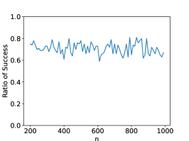
(a) Cross-Attention $n$

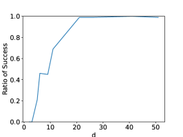
(b) Cross-Attention $d$

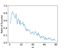
(c) Cross-Attention $m$

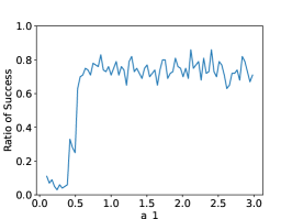
(d) Cross-Attention $a_{1}$

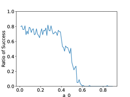
(e) Cross-Attention $a_{0}$

Figure 7: Cross-Attention

We set the dataset as described in Section F.1. For a pair of inputs $(A_{01},A_{02},A_{03})\in\mathcal{D}_{0}$ and $(A_{11},A_{12},A_{13})\in\mathcal{D}_{1}$, we define the event $E_{\mathrm{success}}$ as

$$E_{\mathrm{success}}:= ~{}F_{\exp}(A_{11},A_{12},A_{13})>0$$

$$\land ~{}F_{\operatorname{lin}}(A_{11},A_{12},A_{13})=0$$

$$\land ~{}F_{\exp}(A_{01},A_{02},A_{03})=0$$

$$\land ~{}F_{\operatorname{lin}}(A_{01},A_{02},A_{03})=0.$$

We first fix $X=\mathrm{vec}(I_{d})$, and deploy the numerical experiments for parameters $n$, $d$, $m$, $a_{0}$ and $a_{1}$. To be specific,

• We deploy experiments for $n\in[200,1000]$ with a step size of $10$. For each $n$, we set $d=11$, $\delta=0.01$, $m=\log(n/\delta)$, $a_{0}=0.01$, $a_{1}=3$. For each set of parameters, we iteratively generated models 100 times and recorded the occurrences of successful events denoted as $E_{\mathrm{success}}$. The result can be found in Figure (a) in Figure 7.

• We deploy experiments for $d\in\{2,3,5,6,9,11,21,26,41,51\}$. For each $d$, we set $n=200$, $\delta=0.01$, $m=\log(n/\delta)$, $a_{0}=0.01$, $a_{1}=3$. For each set of parameters, we iteratively generated models 100 times and recorded the occurrences of successful events denoted as $E_{\mathrm{success}}$. The result can be found in Figure (b) in Figure 7.

• We deploy experiments for $m\in[1,80]$ with a step size of $1$. For each $m$, we set $n=200$, $d=11$, $\delta=0.01$, $m=\log(n/\delta)$, $a_{0}=0.01$, $a_{1}=3$. For each set of parameters, we iteratively generated models 100 times and recorded the occurrences of successful events denoted as $E_{\mathrm{success}}$. The result can be found in Figure (c) in Figure 7.

• We deploy experiments for $a_{1}\in[0.1,3]$ with a step size of $0.036$. For each $a_{1}$, we set $n=200$, $d=12$, $\delta=0.01$, $m=\log(n/\delta)$, $a_{0}=0.01$. For each set of parameters, we iteratively generated models 100 times and recorded the occurrences of successful events denoted as $E_{\mathrm{success}}$. The result can be found in Figure (d) in Figure 7.

• We deploy experiments for $a_{0}\in[0.01,0.9]$ with a step size of $0.01$. For each $a_{0}$, we set $n=200$, $d=12$, $\delta=0.01$, $m=\log(n/\delta)$, $a_{0}=0.01$. For each set of parameters, we iteratively generated models 100 times and recorded the occurrences of successful events denoted as $E_{\mathrm{success}}$. The result can be found in Figure (e) in Figure 7.

References

- ACSS [20] Josh Alman, Timothy Chu, Aaron Schild, and Zhao Song. Algorithms and hardness for linear algebra on geometric graphs. In 2020 IEEE 61st Annual Symposium on Foundations of Computer Science (FOCS), pages 541–552. IEEE, 2020.
- AG [23] Pranjal Awasthi and Anupam Gupta. Improving length-generalization in transformers via task hinting. arXiv preprint arXiv:2310.00726, 2023.
- ALS+ [23] Josh Alman, Jiehao Liang, Zhao Song, Ruizhe Zhang, and Danyang Zhuo. Bypass exponential time preprocessing: Fast neural network training via weight-data correlation preprocessing. In NeurIPS. arXiv preprint arXiv:2211.14227, 2023.
- [4] Josh Alman and Zhao Song. Fast attention requires bounded entries. In NeurIPS. arXiv preprint arXiv:2302.13214, 2023.
- [5] Josh Alman and Zhao Song. How to capture higher-order correlations? generalizing matrix softmax attention to kronecker computation. arXiv preprint arXiv:2310.04064, 2023.
- ASA+ [22] Ekin Akyürek, Dale Schuurmans, Jacob Andreas, Tengyu Ma, and Denny Zhou. What learning algorithm is in-context learning? investigations with linear models. arXiv preprint arXiv:2211.15661, 2022.
- [7] Zeyuan Allen-Zhu, Yuanzhi Li, and Zhao Song. A convergence theory for deep learning via over-parameterization. In International Conference on Machine Learning, pages 242–252. PMLR, 2019.
- [8] Zeyuan Allen-Zhu, Yuanzhi Li, and Zhao Song. On the convergence rate of training recurrent neural networks. Advances in neural information processing systems, 32, 2019.
- BAG [20] Satwik Bhattamishra, Kabir Ahuja, and Navin Goyal. On the Ability and Limitations of Transformers to Recognize Formal Languages. In Proceedings of the 2020 Conference on Empirical Methods in Natural Language Processing (EMNLP), pages 7096–7116, Online, November 2020. Association for Computational Linguistics.
- BCE+ [23] Sebastien Bubeck, Varun Chandrasekaran, Ronen Eldan, Johannes Gehrke, Eric Horvitz, Ece Kamar, Peter Lee, Yin Tat Lee, Yuanzhi Li, Scott Lundberg, Harsha Nori, Hamid Palangi, Marco Tulio Ribeiro, and Yi Zhang. Sparks of artificial general intelligence: Early experiments with gpt-4. arXiv preprint arXiv:2305.12712, 2023.
- Bel [22] Yonatan Belinkov. Probing classifiers: Promises, shortcomings, and advances. Computational Linguistics, 48(1):207–219, March 2022.
- BIS [17] Arturs Backurs, Piotr Indyk, and Ludwig Schmidt. On the fine-grained complexity of empirical risk minimization: Kernel methods and neural networks. Advances in Neural Information Processing Systems (NeurIPS), 30, 2017.
- BMR+ [20] Tom Brown, Benjamin Mann, Nick Ryder, Melanie Subbiah, Jared D Kaplan, Prafulla Dhariwal, Arvind Neelakantan, Pranav Shyam, Girish Sastry, Amanda Askell, et al. Language models are few-shot learners. Advances in neural information processing systems, 33:1877–1901, 2020.
- BPG [20] Satwik Bhattamishra, Arkil Patel, and Navin Goyal. On the computational power of transformers and its implications in sequence modeling. In Proceedings of the 24th Conference on Computational Natural Language Learning, pages 455–475, Online, November 2020. Association for Computational Linguistics.
- BPSW [21] Jan van den Brand, Binghui Peng, Zhao Song, and Omri Weinstein. Training (overparametrized) neural networks in near-linear time. In ITCS, 2021.
- BSZ [23] Jan van den Brand, Zhao Song, and Tianyi Zhou. Algorithm and hardness for dynamic attention maintenance in large language models. arXiv preprint arXiv:2304.02207, 2023.
- CDL+ [22] Beidi Chen, Tri Dao, Kaizhao Liang, Jiaming Yang, Zhao Song, Atri Rudra, and Christopher Re. Pixelated butterfly: Simple and efficient sparse training for neural network models. In International Conference on Learning Representations (ICLR), 2022.
- CDW+ [21] Beidi Chen, Tri Dao, Eric Winsor, Zhao Song, Atri Rudra, and Christopher Ré. Scatterbrain: Unifying sparse and low-rank attention. Advances in Neural Information Processing Systems (NeurIPS), 34:17413–17426, 2021.
- CGRS [19] Rewon Child, Scott Gray, Alec Radford, and Ilya Sutskever. Generating long sequences with sparse transformers. arXiv preprint arXiv:1904.10509, 2019.
- Che [18] Lijie Chen. On the hardness of approximate and exact (bichromatic) maximum inner product. In CCC. arXiv preprint arXiv:1802.02325, 2018.
- CJW [19] Lijie Chen, Ce Jin, and R Ryan Williams. Hardness magnification for all sparse np languages. In 2019 IEEE 60th Annual Symposium on Foundations of Computer Science (FOCS), pages 1240–1255. IEEE, 2019.
- CLD+ [20] Krzysztof Choromanski, Valerii Likhosherstov, David Dohan, Xingyou Song, Andreea Gane, Tamas Sarlos, Peter Hawkins, Jared Davis, Afroz Mohiuddin, Lukasz Kaiser, et al. Rethinking attention with performers. arXiv preprint arXiv:2009.14794, 2020.
- CLMY [21] HanQin Cai, Yuchen Lou, Daniel Mckenzie, and Wotao Yin. A zeroth-order block coordinate descent algorithm for huge-scale black-box optimization. arXiv preprint arXiv:2102.10707, 2021.
- CLP+ [21] Beidi Chen, Zichang Liu, Binghui Peng, Zhaozhuo Xu, Jonathan Lingjie Li, Tri Dao, Zhao Song, Anshumali Shrivastava, and Re.Mongoose Christopher. A learnable lsh framework for efficient neural network training. International Conference on Learning Representation, 2021.
- CND+ [22] Aakanksha Chowdhery, Sharan Narang, Jacob Devlin, Maarten Bosma, Gaurav Mishra, Adam Roberts, Paul Barham, Hyung Won Chung, Charles Sutton, Sebastian Gehrmann, et al. Palm: Scaling language modeling with pathways. arXiv preprint arXiv:2204.02311, 2022.
- DCL+ [22] Tri Dao, Beidi Chen, Kaizhao Liang, Jiaming Yang, Zhao Song, Atri Rudra, and Christopher Re. Pixelated butterfly: Simple and efficient sparse training for neural network models. In ICLR. arXiv preprint arXiv:2112.00029, 2022.
- DCLT [18] Jacob Devlin, Ming-Wei Chang, Kenton Lee, and Kristina Toutanova. Bert: Pre-training of deep bidirectional transformers for language understanding. arXiv preprint arXiv:1810.04805, 2018.
- DGS [23] Yichuan Deng, Yeqi Gao, and Zhao Song. Solving tensor low cycle rank approximation. arXiv preprint arXiv:2304.06594, 2023.
- DGV+ [18] Mostafa Dehghani, Stephan Gouws, Oriol Vinyals, Jakob Uszkoreit, and Łukasz Kaiser. Universal transformers. arXiv preprint arXiv:1807.03819, 2018.
- DKOD [20] Giannis Daras, Nikita Kitaev, Augustus Odena, and Alexandros G Dimakis. Smyrf-efficient attention using asymmetric clustering. Advances in Neural Information Processing Systems (NeurIPS), 33:6476–6489, 2020.
- DLMS [23] Yichuan Deng, Zhihang Li, Sridhar Mahadevan, and Zhao Song. Zero-th order algorithm for softmax attention optimization. arXiv preprint arXiv:2307.08352, 2023.
- DLS [23] Yichuan Deng, Zhihang Li, and Zhao Song. Attention scheme inspired softmax regression. arXiv preprint arXiv:2304.10411, 2023.
- DMS [23] Yichuan Deng, Sridhar Mahadevan, and Zhao Song. Randomized and deterministic attention sparsification algorithms for over-parameterized feature dimension. arxiv preprint: arxiv 2304.03426, 2023.
- DSX [23] Yichuan Deng, Zhao Song, and Shenghao Xie. Convergence of two-layer regression with nonlinear units. arXiv preprint arXiv:2308.08358, 2023.
- DZPS [19] Simon S Du, Xiyu Zhai, Barnabas Poczos, and Aarti Singh. Gradient descent provably optimizes over-parameterized neural networks. arXiv preprint arXiv:1810.02054, 2019.
- EGKZ [21] Benjamin L Edelman, Surbhi Goel, Sham Kakade, and Cyril Zhang. Inductive biases and variable creation in self-attention mechanisms. arXiv preprint arXiv:2110.10090, 2021.
- EGZ [20] Javid Ebrahimi, Dhruv Gelda, and Wei Zhang. How can self-attention networks recognize Dyck-n languages? In Findings of the Association for Computational Linguistics: EMNLP 2020, pages 4301–4306, Online, November 2020. Association for Computational Linguistics.
- GMS [23] Yeqi Gao, Sridhar Mahadevan, and Zhao Song. An over-parameterized exponential regression. arXiv preprint arXiv:2303.16504, 2023.
- GSWY [23] Yeqi Gao, Zhao Song, Weixin Wang, and Junze Yin. A fast optimization view: Reformulating single layer attention in llm based on tensor and svm trick, and solving it in matrix multiplication time. arXiv preprint arXiv:2309.07418, 2023.
- GSX [23] Yeqi Gao, Zhao Song, and Shenghao Xie. In-context learning for attention scheme: from single softmax regression to multiple softmax regression via a tensor trick. arXiv preprint arXiv:2307.02419, 2023.
- GSY [23] Yeqi Gao, Zhao Song, and Junze Yin. Gradientcoin: A peer-to-peer decentralized large language models. arXiv preprint arXiv:2308.10502, 2023.
- GSYZ [23] Yeqi Gao, Zhao Song, Xin Yang, and Ruizhe Zhang. Fast quantum algorithm for attention computation. arXiv preprint arXiv:2307.08045, 2023.
- GTLV [22] Shivam Garg, Dimitris Tsipras, Percy Liang, and Gregory Valiant. What can transformers learn in-context? a case study of simple function classes. arXiv preprint arXiv:2208.01066, 2022.
- HJK+ [23] Insu Han, Rajesh Jarayam, Amin Karbasi, Vahab Mirrokni, David P. Woodruff, and Amir Zandieh. Hyperattention: Long-context attention in near-linear time. arXiv preprint arXiv:2310.05869, 2023.
- HL [19] John Hewitt and Percy Liang. Designing and interpreting probes with control tasks. In Proceedings of the 2019 Conference on Empirical Methods in Natural Language Processing and the 9th International Joint Conference on Natural Language Processing (EMNLP-IJCNLP), pages 2733–2743, Hong Kong, China, November 2019. Association for Computational Linguistics.
- Hoe [63] Wassily Hoeffding. Probability inequalities for sums of bounded random variables. Journal of the American Statistical Association, 58(301):13–30, 1963.
- Inc [23] Adobe Inc. Adobe firefly. https://www.adobe.com/sensei/generative-ai/firefly.html, 2023.
- JX [23] Ce Jin and Yinzhan Xu. Removing additive structure in 3sum-based reductions. In Proceedings of the 55th Annual ACM Symposium on Theory of Computing, pages 405–418, 2023.
- KKL [20] Nikita Kitaev, Lukasz Kaiser, and Anselm Levskaya. Reformer: The efficient transformer. arXiv preprint arXiv: 2001.04451, 2020.
- KMZ [23] Praneeth Kacham, Vahab Mirrokni, and Peilin Zhong. Polysketchformer: Fast transformers via sketches for polynomial kernels. arXiv preprint arXiv:2310.01655, 2023.
- KVPF [20] Angelos Katharopoulos, Apoorv Vyas, Nikolaos Pappas, and François Fleuret. Transformers are rnns: Fast autoregressive transformers with linear attention. In International conference on machine learning, pages 5156–5165. PMLR, 2020.
- LCZ+ [23] Langming Liu, Liu Cai, Chi Zhang, Xiangyu Zhao, Jingtong Gao, Wanyu Wang, Yifu Lv, Wenqi Fan, Yiqi Wang, Ming He, et al. Linrec: Linear attention mechanism for long-term sequential recommender systems. In Proceedings of the 46th International ACM SIGIR Conference on Research and Development in Information Retrieval, pages 289–299, 2023.
- LFS+ [17] Zhouhan Lin, Minwei Feng, Cicero Nogueira dos Santos, Mo Yu, Bing Xiang, Bowen Zhou, and Yoshua Bengio. A structured self-attentive sentence embedding. arXiv preprint arXiv:1703.03130, 2017.
- LL [18] Yuanzhi Li and Yingyu Liang. Learning overparameterized neural networks via stochastic gradient descent on structured data. Advances in neural information processing systems, 31, 2018.
- LLH+ [23] Hong Liu, Zhiyuan Li, David Hall, Percy Liang, and Tengyu Ma. Sophia: A scalable stochastic second-order optimizer for language model pre-training. arXiv preprint arXiv:2305.14342, 2023.
- LOG+ [19] Yinhan Liu, Myle Ott, Naman Goyal, Jingfei Du, Mandar Joshi, Danqi Chen, Omer Levy, Mike Lewis, Luke Zettlemoyer, and Veselin Stoyanov. Roberta: A robustly optimized bert pretraining approach. arXiv preprint arXiv:1907.11692, 2019.
- LSDZ [20] Rui Li, Jianlin Su, Chenxi Duan, and Shunyi Zheng. Linear attention mechanism: An efficient attention for semantic segmentation. arXiv preprint arXiv:2007.14902, 2020.
- LSZ [23] Zhihang Li, Zhao Song, and Tianyi Zhou. Solving regularized exp, cosh and sinh regression problems. arXiv preprint arXiv:2303.15725, 2023.
- LWD+ [23] Zichang Liu, Jue Wang, Tri Dao, Tianyi Zhou, Binhang Yuan, Zhao Song, Anshumali Shrivastava, Ce Zhang, Yuandong Tian, Christopher Re, and Beidi Chen. Deja vu: Contextual sparsity for efficient llms at inference time. In ICML, 2023.
- Man [23] James Manyika. An overview of bard: an early experiment with generative ai. Technical report, Tech. rep., Technical report, Google AI, 2023.
- MDA [22] Gary Marcus, Ernest Davis, and Scott Aaronson. A very preliminary analysis of dall-e 2. arXiv preprint arXiv:2204.13807, 2022.
- MGN+ [23] Sadhika Malladi, Tianyu Gao, Eshaan Nichani, Alex Damian, Jason D Lee, Danqi Chen, and Sanjeev Arora. Fine-tuning language models with just forward passes. arXiv preprint arXiv:2305.17333, 2023.
- MOSW [22] Alexander Munteanu, Simon Omlor, Zhao Song, and David Woodruff. Bounding the width of neural networks via coupled initialization a worst case analysis. In International Conference on Machine Learning, pages 16083–16122. PMLR, 2022.
- Ope [23] OpenAI. Gpt-4 technical report. arXiv preprint arXiv:2303.08774, 2023.
- PMB [19] Jorge Pérez, Javier Marinković, and Pablo Barceló. On the turing completeness of modern neural network architectures. arXiv preprint arXiv:1901.03429, 2019.
- PMXA [23] Abhishek Panigrahi, Sadhika Malladi, Mengzhou Xia, and Sanjeev Arora. Trainable transformer in transformer. arXiv preprint arXiv:2307.01189, 2023.
- PSZA [23] Abhishek Panigrahi, Nikunj Saunshi, Haoyu Zhao, and Sanjeev Arora. Task-specific skill localization in fine-tuned language models. arXiv preprint arXiv:2302.06600, 2023.
- PTDU [16] Ankur P Parikh, Oscar Täckström, Dipanjan Das, and Jakob Uszkoreit. A decomposable attention model for natural language inference. arXiv preprint arXiv:1606.01933, 2016.
- RSM+ [23] Rafael Rafailov, Archit Sharma, Eric Mitchell, Stefano Ermon, Christopher D.Manning, and Chelsea Finn. Direct preference optimization: Your language model is secretly a reward model. arXiv preprint arXiv:2305.18290, 2023.
- SHT [23] Clayton Sanford, Daniel Hsu, and Telgarsky. Representational strengths and limitations of transformers. arXiv preprint arXiv:2306.02896, 2023.
- SY [19] Zhao Song and Xin Yang. Quadratic suffices for over-parametrization via matrix chernoff bound. arXiv preprint arXiv:1906.03593, 2019.
- SZKS [21] Charlie Snell, Ruiqi Zhong, Dan Klein, and Jacob Steinhardt. Approximating how single head attention learns. arXiv preprint arXiv:2103.07601, 2021.
- [73] Zhuoran Shen, Mingyuan Zhang, Haiyu Zhao, Shuai Yi, and Hongsheng Li. Efficient attention: Attention with linear complexities. In Proceedings of the IEEE/CVF winter conference on applications of computer vision, pages 3531–3539, 2021.
- [74] Zhao Song, Lichen Zhang, and Ruizhe Zhang. Training multi-layer over-parametrized neural network in subquadratic time. arXiv preprint arXiv:2112.07628, 2021.
- TDFH+ [22] Romal Thoppilan, Daniel De Freitas, Jamie Hall, Noam Shazeer, Apoorv Kulshreshtha, Heng-Tze Cheng, Alicia Jin, Taylor Bos, Leslie Baker, Yu Du, et al. Lamda: Language models for dialog applications. arXiv preprint arXiv:2201.08239, 2022.
- TDP [19] Ian Tenney, Dipanjan Das, and Ellie Pavlick. BERT rediscovers the classical NLP pipeline. In Proceedings of the 57th Annual Meeting of the Association for Computational Linguistics, pages 4593–4601, Florence, Italy, July 2019. Association for Computational Linguistics.
- TLI+ [23] Hugo Touvron, Thibaut Lavril, Gautier Izacard, Xavier Martinet, Marie-Anne Lachaux, Timothée Lacroix, Baptiste Rozière, Naman Goyal, Eric Hambro, Faisal Azhar, et al. Llama: Open and efficient foundation language models. arXiv preprint arXiv:2302.13971, 2023.
- TMS+ [23] Hugo Touvron, Louis Martin, Kevin Stone, Peter Albert, Amjad Almahairi, Yasmine Babaei, Nikolay Bashlykov, Soumya Batra, Prajjwal Bhargava, Shruti Bhosale, et al. Llama 2: Open foundation and fine-tuned chat models. arXiv preprint arXiv:2307.09288, 2023.
- VB [19] Jesse Vig and Yonatan Belinkov. Analyzing the structure of attention in a transformer language model. In Proceedings of the 2019 ACL Workshop BlackboxNLP: Analyzing and Interpreting Neural Networks for NLP, pages 63–76, Florence, Italy, August 2019. Association for Computational Linguistics.
- VBC [20] James Vuckovic, Aristide Baratin, and Remi Tachet des Combes. A mathematical theory of attention. arXiv preprint arXiv:2007.02876, 2020.
- VSP+ [17] Ashish Vaswani, Noam Shazeer, Niki Parmar, Jakob Uszkoreit, Llion Jones, Aidan N Gomez, Łukasz Kaiser, and Illia Polosukhin. Attention is all you need. Advances in neural information processing systems, 30, 2017.
- WCM [21] Colin Wei, Yining Chen, and Tengyu Ma. Statistically meaningful approximation: a case study on approximating turing machines with transformers. arXiv preprint arXiv:2107.13163, 2021.
- WLK+ [20] Sinong Wang, Belinda Z Li, Madian Khabsa, Han Fang, and Hao Ma. Linformer: Self-attention with linear complexity. arXiv preprint arXiv:2006.04768, 2020.
- WTB+ [22] Jason Wei, Yi Tay, Rishi Bommasani, Colin Raffel, Barret Zoph, Sebastian Borgeaud, Dani Yogatama, Maarten Bosma, Denny Zhou, Donald Metzler, et al. Emergent abilities of large language models. arXiv preprint arXiv:2206.07682, 2022.
- WZW [23] Xinyi Wang, Wanrong Zhu, and William Yang Wang. Large language models are implicitly topic models: Explaning and finding good demonstrations for in-context learning. arXiv preprint arXiv:2301.11916, 2023.
- YBR+ [20] Chulhee Yun, Srinadh Bhojanapalli, Ankit Singh Rawat, Sashank Reddi, and Sanjiv Kumar. Are transformers universal approximators of sequence-to-sequence functions? In International Conference on Learning Representations, 2020.
- YCRI [22] Ann Yuan, Andy Coenen, Emily Reif, and Daphne Ippolito. Wordcraft: story writing with large language models. In 27th International Conference on Intelligent User Interfaces, pages 841–852, 2022.
- YDY+ [19] Zhilin Yang, Zihang Dai, Yiming Yang, Jaime Carbonell, Russ R Salakhutdinov, and Quoc V Le. Xlnet: Generalized autoregressive pretraining for language understanding. Advances in neural information processing systems, 32, 2019.
- YPPN [21] Shunyu Yao, Binghui Peng, Christos Papadimitriou, and Karthik Narasimhan. Self-attention networks can process bounded hierarchical languages. In Proceedings of the 59th Annual Meeting of the Association for Computational Linguistics and the 11th International Joint Conference on Natural Language Processing (Volume 1: Long Papers), pages 3770–3785, Online, August 2021. Association for Computational Linguistics.
- ZBB+ [22] Yi Zhang, Arturs Backurs, Sébastien Bubeck, Ronen Eldan, Suriya Gunasekar, and Tal Wagner. Unveiling transformers with lego: a synthetic reasoning task, 2022.
- ZFB [23] Ruiqi Zhang, Spencer Frei, and Peter L Bartlett. Trained transformers learn linear models in-context. arXiv preprint arXiv:2306.09927, 2023.
- ZHDK [23] Amir Zandieh, Insu Han, Majid Daliri, and Amin Karbasi. Kdeformer: Accelerating transformers via kernel density estimation. In ICML. arXiv preprint arXiv:2302.02451, 2023.
- ZKV+ [20] Jingzhao Zhang, Sai Praneeth Karimireddy, Andreas Veit, Seungyeon Kim, Sashank Reddi, Sanjiv Kumar, and Suvrit Sra. Why are adaptive methods good for attention models? Advances in Neural Information Processing Systems, 33:15383–15393, 2020.
- ZPGA [23] Haoyu Zhao, Abhishek Panigrahi, Rong Ge, and Sanjeev Arora. Do transformers parse while predicting the masked word? arXiv preprint arXiv:2303.08117, 2023.
- ZRG+ [22] Susan Zhang, Stephen Roller, Naman Goyal, Mikel Artetxe, Moya Chen, Shuohui Chen, Christopher Dewan, Mona Diab, Xian Li, Xi Victoria Lin, et al. Opt: Open pre-trained transformer language models. arXiv preprint arXiv:2205.01068, 2022.
- ZSJ+ [17] Kai Zhong, Zhao Song, Prateek Jain, Peter L Bartlett, and Inderjit S Dhillon. Recovery guarantees for one-hidden-layer neural networks. In International conference on machine learning, pages 4140–4149. PMLR, 2017.
- ZWK [22] Lin Zheng, Chong Wang, and Lingpeng Kong. Linear complexity randomized self-attention mechanism. In International Conference on Machine Learning, pages 27011–27041. PMLR, 2022.