A Symbolic Language
for Interpreting Decision Trees

Abstract

The recent development of formal explainable AI has disputed the folklore claim “decision trees are readily interpretable models”, showing different interpretability queries that are computationally hard on decision trees, as well as proposing different methods to deal with them in practice. Nonetheless, no single explainability query or score works as a “silver bullet” that is appropriate for every context and end-user. This naturally suggests the possibility of “interpretability languages” in which a wide variety of queries can be expressed, giving control to the end-user to tailor queries to their particular needs. In this context, our work presents ExplainDT, a symbolic language for interpreting decision trees.  ExplainDT is rooted in a carefully constructed fragment of first-order logic that we call StratiFOILed. StratiFOILed balances expressiveness and complexity of evaluation, allowing for the computation of many post-hoc explanations — both local (e.g., abductive and contrastive explanations) and global ones (e.g., feature relevance) — while remaining in the Boolean Hierarchy over NP. Furthermore, StratiFOILed queries can be written as a Boolean combination of NP-problems, thus allowing us to evaluate them in practice with a constant number of calls to a SAT solver. On the theoretical side, our main contribution is an in-depth analysis of the expressiveness and complexity of StratiFOILed, while on the practical side, we provide an optimized implementation for encoding StratiFOILed queries as propositional formulas, together with an experimental study on its efficiency.

1 Introduction

Context.

The increasing need to comprehend the decisions made by machine learning (ML) models has fostered a large body of research in explainable AI (XAI) methods [42], leading to the introduction of numerous queries and scores that aim to explain individual predictions produced by such models. For example, several methods aim to measure the contribution of a feature, or a set of features, to the output of an ML model, thus enabling users to identify the most influential features in shaping the model’s decision around a given input [46, 19, 38].

Nonetheless, it is often not a single query or score, but a combination of them, that provides the best explanation [16, 41]. Furthermore, it has been shown that some widely used explainability scores, believed to be theoretically mature and robust, may behave counterintuitively in certain situations [24, 21, 11, 51, 32]. This state of affairs has raised a call for developing explainability languages: general-purpose languages that allow users the flexibility to interact with an ML model, by posing different queries, in search of the best explanation. A first attempt in this direction was carried out by Arenas et al. [2], who designed a simple explainability language based on first-order logic, called FOIL for first-order interpretability logic, that was able to express some basic explainability queries.

However, as noted by the authors of [2], the primary purpose of FOIL was not to serve as a practical explainability language but as a foundation upon which such languages could be constructed. To date, nevertheless, we have no complete understanding of why FOIL is not a good practical language for explainability, nor what needs to be added to it in order to make it a more effective tool for performing such tasks. To gain a deeper understanding of this issue, we introduce two desiderata that any language used for explainability queries should meet: (1) Rich expressive power: The language should be able to express a broad range of explainability queries commonly used in practice; (2) Efficiency: The computational complexity of the language used to express explainability queries must be manageable. Specifically, we require that queries can be evaluated with a constant number of calls to an NP oracle, which may enable the use of SAT solvers for query evaluation. SAT solvers are a mature technology that is effective in computing explanations for various ML models [30, 55, 27].

Theoretical contributions.

We start by assessing the suitability of FOIL as an explainability language, with a specific emphasis on its ability to meet the first criterion in our desiderata. We show that there are crucial explainability queries that cannot be expressed in this language. For instance, the query known as the minimum sufficient reason [48, 6] cannot be expressed in FOIL. This query takes an input $\mathbf{e}$ to a machine learning model $\mathcal{M}$ and requests a subset $S$ of its features, with the smallest possible cardinality, that justifies the output of the model on said input. In other words, the output of $\mathcal{M}$ on inputs that coincide with $\mathbf{e}$ on the features from $S$ must always be the same.

In view of this drawback, we propose a natural extension of the FOIL language, which we call $\textsc{FOIL}^{+}$. We demonstrate that $\textsc{FOIL}^{+}$ can express a broad range of explainability queries commonly used in practice, including the minimum sufficient reason. Importantly, $\textsc{FOIL}^{+}$ is model-agnostic, meaning it does not depend on the specific type of machine learning model being employed.

Next, we explore the computational cost of evaluating $\textsc{FOIL}^{+}$ queries to gain understanding of the second condition in our list of requirements. Our focus is on the evaluation problem over decision trees, a class of ML models that have been extensively studied for explainability in the literature [6, 28, 2, 30, 29, 3]. It is known that there are FOIL queries that are ${\rm NP}$-hard to evaluate on decision trees [2]. However, it remains unclear whether every $\textsc{FOIL}^{+}$ query over decision trees can be evaluated by a constant number of calls to ${\rm NP}$ oracles. We show that, under some widely believed complexity assumptions, this is not the case. Specifically, we show that the $\textsc{FOIL}^{+}$ evaluation problem over decision trees is hard for each level of the polynomial hierarchy, which goes well beyond the problems that can be solved with a constant, or even polynomial, number of calls to an ${\rm NP}$ oracle.

Based on this negative result, we identify a language StratiFOILed that satisfies our desiderata: (a) it is able to express a broad range of explainability queries commonly used in practice; in fact, all the examples we present of explainability queries that can be expressed in $\textsc{FOIL}^{+}$ can also be expressed in StratiFOILed; and (b) every query expressible in StratiFOILed can be evaluated with a constant number of calls to an ${\rm NP}$ oracle. The language StratiFOILed is so named because it is a stratified version of $\textsc{FOIL}^{+}$, but which allows quantification over a specific class of objects that cannot be defined in $\textsc{FOIL}^{+}$. Unlike $\textsc{FOIL}^{+}$, the language StratiFOILed is model-specific, as the class of objects over which we allow this extended quantification to range over is characteristic of the decision trees. This allows us to define the language StratiFOILed in a simple and elegant way.

Practical contributions.

We present an implementation of ExplainDT, a minimalistic high-level language that can be used to interpret trained decision trees. ExplainDT  queries are compiled into StratiFOILed formulas, then run through a simplifier module, to then encode a CNF formula whose satisfiability captures the truth-value of the StratiFOILed formula. Such CNF formulas are later fed to a SAT solver, whose answer is given back to the user, thus closing the loop. Figure 2 illustrates the intended workflow when using ExplainDT. Our entire implementation, together with the necessary code to reproduce our experiments, is available in the repository .

Related work.

Our work is rooted in the area of formal XAI [40, 13, 39], which aims to deliver trust-worthy explanations through well-defined semantics, meaning that each kind of explanation has a precise mathematical definition, thus avoiding the pitfalls of explanations that do not make sense or are unfaithful to the underlying models  [47]. The problem of explaining decision trees, as well as their generalization to random forests, has received significant attention within the community [12, 30, 28, 6, 29, 3, 2, 4]. The theoretical line of work within formal XAI that is closest to our work is that Liu and Lorini [36, 35, 34], which also concerns logic-based languages for explainability. The main differences between our work and that of Liu and Lorini are: (i) we provide an implementation of our language, (ii) we use classical first-order logic as opposed to modal logic, and (iii) the complexity of evaluation is much lower in our logic. On the other hand, the practical line of work that is closest to ours is that of libraries for computing abductive and contrastive explanations for tree-based models, such as PyXAI [5] and XReason [24, 25, 22]. However, while PyXAI and XReason provide support only for a finite number of pre-defined queries, ExplainDT allows writing an infinite family of different queries. Finally, our implementation based on SAT encodings is related to a wide range of work using SAT-solving for explainability [28, 3, 26, 43, 40].

Figure 1: High-level diagram of the ExplainDT workflow.

Figure 2: Example of a decision tree of dimension $4$.

2 Background

Models and instances.

We use an abstract notion of a model of dimension $n$, and define it as a Boolean function $\mathcal{M}:\{0,1\}^{n}\to\{0,1\}$. We write ${\rm dim}(\mathcal{M})$ for the dimension of a model $\mathcal{M}$. A partial instance of dimension $n$ is a tuple $\mathbf{e}\in\{0,1,\bot\}^{n}$, where $\bot$ is used to represent undefined features. We define $\mathbf{e}_{\bot}=\{i\in\{1,\dots,n\}\mid\mathbf{e}[i]=\bot\}$. An instance of dimension $n$ is a tuple $\mathbf{e}\in\{0,1\}^{n}$. That is, an instance is a partial instance without undefined features. Given partial instances $\mathbf{e}_{1}$, $\mathbf{e}_{2}$ of dimension $n$, we say that $\mathbf{e}_{1}$ is subsumed by $\mathbf{e}_{2}$ if for every $i\in\{1,\ldots,n\}$ with $\mathbf{e}_{1}[i]\neq\bot$, it holds that $\mathbf{e}_{1}[i]=\mathbf{e}_{2}[i]$. That is, it is possible to obtain $\mathbf{e}_{2}$ from $\mathbf{e}_{1}$ by replacing some unknown values. For example, $(1,\bot)$ is subsumed by $(1,0)$, but it is not subsumed by $(0,0)$. A partial instance $\mathbf{e}$ can be seen as a compact representation of the set of instances $\mathbf{e}^{\prime}$ such that $\mathbf{e}$ is subsumed by $\mathbf{e}^{\prime}$, where such instances $\mathbf{e}^{\prime}$ are called the completions of $\mathbf{e}$.

Decision trees.

A decision tree (cf. Figure 2) over instances of dimension $n$ is a rooted directed tree $\mathcal{T}$ with labels on edges and nodes such that: (i) each leaf is labeled with $\mathbf{true}$ or $\mathbf{false}$; (ii) each internal node (a node that is not a leaf) is labeled with a feature $i\in\{1,\dots,n\}$; (iii) each internal node has two outgoing edges, one labeled $0$ and the another one labeled $1$, and (iv) in every path from the root to a leaf, no two nodes on that path have the same label. Every instance $\mathbf{e}\in\{0,1\}^{n}$ defines a unique path $\pi_{\mathbf{e}}=u_{1}\cdots u_{k}$ from the root $u_{1}$ to a leaf $u_{k}$ of $\mathcal{T}$ such that: if the label of $u_{i}$ is $j\in\{1,\dots,n\}$, where $i\in\{1,\ldots,k-1\}$, then the edge from $u_{i}$ to $u_{i+1}$ is labeled with $\mathbf{e}[j]$. Further, the instance $\mathbf{e}$ is positive, denoted by $\mathcal{T}(\mathbf{e})=1$, if the label of $u_{k}$ is $\mathbf{true}$; otherwise the instance $\mathbf{e}$ is negative, which is denoted by $\mathcal{T}(\mathbf{e})=0$. For example, for the decision tree $\mathcal{T}$ in Figure 2 and instances $\mathbf{e}_{1}=(0,0,1,1)$ and $\mathbf{e}_{2}=(0,1,1,0)$, it holds that $\mathcal{T}(\mathbf{e}_{1})=1$ and $\mathcal{T}(\mathbf{e}_{2})=0$.

3 The FOIL Logic

FOIL was introduced in [2], and it is simply first-order logic over two relations on the set of partial instances of a given dimension: A unary relation Pos which indicates the value of an instance in a model, and a binary relation $\subseteq$ that represents the subsumption relation among partial instances.

We assume familiarity with the syntax and semantics of first-order logic (see the appendix for a review of these concepts). In particular, given a vocabulary $\sigma$ consisting of relations $R_{1}$, $\ldots$, $R_{\ell}$, recall that a structure $\mathfrak{A}$ over $\sigma$ consists of a domain, where quantifiers are instantiated, and an interpretation for each relation $R_{i}$. Moreover, given a first-order formula $\varphi$ defined over the vocabulary $\sigma$, we write $\varphi(x_{1},\ldots,x_{k})$ to indicate that $\{x_{1},\ldots,x_{k}\}$ is the set of free variables of $\varphi$. Finally, given a structure $\mathfrak{A}$ over the vocabulary $\sigma$ and elements $a_{1}$, $\ldots$, $a_{k}$ in the domain of $\mathfrak{A}$, we use $\mathfrak{A}\models\varphi(a_{1},\ldots,a_{k})$ to indicate that formula $\varphi$ is satisfied by $\mathfrak{A}$ when each variable $x_{i}$ is replaced by element $a_{i}$ ($1\leq i\leq k$).

Consider a model $\mathcal{M}$ with ${\rm dim}(\mathcal{M})=n$. The structure $\mathfrak{A}_{\mathcal{M}}$ representing $\mathcal{M}$ over the vocabulary formed by Pos and $\subseteq$ is defined as follows. The domain of $\mathfrak{A}_{\mathcal{M}}$ is the set $\{0,1,\bot\}^{n}$ of all partial instances of dimension $n$. An instance $\mathbf{e}\in\{0,1\}^{n}$ is in the interpretation of Pos in $\mathfrak{A}_{\mathcal{M}}$ if and only if $\mathcal{M}(\mathbf{e})=1$, and no partial instance including undefined features is contained in the interpretation of Pos. Moreover, a pair $(\mathbf{e}_{1},\mathbf{e}_{2})$ is in the interpretation of relation $\subseteq$ in $\mathfrak{A}_{\mathcal{M}}$ if and only if $\mathbf{e}_{1}$ is subsumed by $\mathbf{e}_{2}$. Then given a formula $\varphi(x_{1},\ldots,x_{k})$ in FOIL and partial instances $\mathbf{e}_{1}$, $\ldots$, $\mathbf{e}_{k}$ of dimension $n$, model $\mathcal{M}$ is said to satisfy $\varphi(\mathbf{e}_{1},\ldots,\mathbf{e}_{k})$, denoted by $\mathcal{M}\models\varphi(\mathbf{e}_{1},\ldots,\mathbf{e}_{k})$, if $\mathfrak{A}_{\mathcal{M}}\models\varphi(\mathbf{e}_{1},\ldots,\mathbf{e}_{k})$. Notice that for a decision tree $\mathcal{T}$, the structure $\mathfrak{A}_{\mathcal{T}}$ can be exponentially larger than $\mathcal{T}$. Hence, $\mathfrak{A}_{\mathcal{T}}$ is a theoretical construction needed to formally define the semantics of FOIL, but that should not be built when verifying in practice if a formula $\varphi$ is satisfied by $\mathcal{T}$.

3.1 Expressing properties in FOIL

We give several examples of how FOIL can be used to express some natural explainability queries on models. In these examples we make use of the following FOIL formula: $\textsc{Full}(x)=\forall y\,(x\subseteq y\,\rightarrow\,y\subseteq x)$. Notice that if $\mathcal{M}$ is a model and $\mathbf{e}$ is a partial instance, then $\mathcal{M}\models\textsc{Full}(\mathbf{e})$ if and only if $\mathbf{e}$ is also an instance (i.e., it has no undefined features). We also use the formula

$$\textsc{AllPos}(x)\ =\ \forall y\,\big{(}(x\subseteq y\wedge\textsc{Full}(y))\,\rightarrow\,\textsc{Pos}(y)\big{)},$$

such that $\mathcal{M}\models\textsc{AllPos}(\mathbf{e})$ if and only if every completion $\mathbf{e}^{\prime}$ of $\mathbf{e}$ is a positive instance of $\mathcal{M}$. Analogously, we define a formula $\textsc{AllNeg}(x)$.

Sufficient reasons.

A sufficient reason (SR) for an instance $\mathbf{e}$ over a model $\mathcal{M}$ is a partial instance $\mathbf{e}^{\prime}$ such that $\mathbf{e}^{\prime}\subseteq\mathbf{e}$ and each completion of $\mathbf{e}^{\prime}$ takes the same value over $\mathcal{M}$ as $\mathbf{e}$. We can define SRs in FOIL by means of the following formula:

$$\textsc{SR}(x,y)\ =\ \textsc{Full}(x)\wedge\,y\subseteq x\,\wedge\,\forall z\,\big{(}(y\subseteq z\wedge\textsc{Full}(z))\,\rightarrow\,(\textsc{Pos}(z)\leftrightarrow\textsc{Pos}(x))\big{)}.$$

In fact, it is easy to see that $\mathcal{M}\models\textsc{SR}(\mathbf{e},\mathbf{e}^{\prime})$ if and only if $\mathbf{e}^{\prime}$ is a SR for $\mathbf{e}$ over $\mathcal{M}$.

Notice that $\mathbf{e}$ is always a SR for itself. However, we are typically interested in SRs that satisfy some optimality criterion. A common such criterion is that of being minimal [48, 28, 6, 2]. Formally, $\mathbf{e}^{\prime}$ is a minimal SR for $\mathbf{e}$ over $\mathcal{M}$, if $\mathbf{e}^{\prime}$ is a SR for $\mathbf{e}$ over $\mathcal{M}$ and there is no partial instance $\mathbf{e}^{\prime\prime}$ that is properly subsumed by $\mathbf{e}^{\prime}$ that is also a SR for $\mathbf{e}$. Let us write $x\subsetneq y$ for $x\subseteq y\wedge\neg(y\subseteq x)$. Then for

$$\textsc{MinimalSR}(x,y)\ =\ \textsc{SR}(x,y)\,\wedge\,\forall z\,(z\subsetneq y\,\rightarrow\neg\textsc{SR}(x,z)),$$

we have that $\mathcal{M}\models\textsc{MinimalSR}(\mathbf{e},\mathbf{e}^{\prime})$ if and only if $\mathbf{e}^{\prime}$ is a minimal SR for $\mathbf{e}$ over $\mathcal{M}$. Minimal SRs have also been called prime implicant or abductive explanations in the literature [23, 38].

Feature Relevancy.

A standard global interpretability question about an ML model is to decide which features are relevant to its decisions [20, 14]. Such a notion can be defined in FOIL as follows:

$$\textsc{RFS}(x)\ =\ \forall y\,\big{(}\textsc{SUF}(x,y)\,\rightarrow\,(\textsc{AllPos}(y)\vee\textsc{AllNeg}(y))\big{)},$$ (1)

where $\textsc{SUF}(x,y)$ is a FOIL formula (SUF stands for same undefined features) such that $\mathcal{M}\models\textsc{SUF}(\mathbf{e},\mathbf{e}^{\prime})$ if and only if $\mathbf{e}_{\bot}=\mathbf{e}^{\prime}_{\bot}$, i.e., the sets of undefined features in $\mathbf{e}$ and $\mathbf{e}^{\prime}$ are the same (see the appendix for a definition of this formula). Then we have that $\mathcal{M}\models\textsc{RFS}(\mathbf{e})$ if and only if for every $\mathbf{e}^{\prime}$ with $\mathbf{e}_{\bot}=\mathbf{e}^{\prime}_{\bot}$, all completions of $\mathbf{e}^{\prime}$ receive the same classification over $\mathcal{M}$. In other words, the output of the model on each instance is invariant to the features that are undefined in $\mathbf{e}$. We call this a Relevant Feature Set (RFS). For example, for the decision tree $\mathcal{T}$ shown in Figure 2, the set of features $\{1,3,4\}$ is an RFS, as the output of the model does not depend on feature 2. In particular, for the instances $\mathbf{e}_{1}=(0,0,0,0)$ and $\mathbf{e}_{2}=(0,1,0,0)$, we have that $\mathcal{T}(\mathbf{e}_{1})=\mathcal{T}(\mathbf{e}_{2})=1$, while for the instances $\mathbf{e}_{3}=(1,0,1,0)$ and $\mathbf{e}_{4}=(1,1,1,0)$, we have that $\mathcal{T}(\mathbf{e}_{3})=\mathcal{T}(\mathbf{e}_{4})=0$, so that the output of the model on these instances does not depend on feature 2. As before, we can also express that $\mathbf{e}$ is minimal with respect to feature relevancy using the formula: $\textsc{MinimalRFS}(x)=\textsc{RFS}(x)\,\wedge\,\forall y\,(y\subsetneq x\,\rightarrow\neg\textsc{RFS}(y))$.

3.2 Expressiveness limitations of FOIL

In some scenarios we want to express a stronger condition for SRs and RFSs: not only that they are minimal, but also that they are minimum. Formally, a SR $\mathbf{e}^{\prime}$ for $\mathbf{e}$ over $\mathcal{M}$ is minimum, if there is no SR $\mathbf{e}^{\prime\prime}$ for $\mathbf{e}$ over $\mathcal{M}$ with $|\mathbf{e}^{\prime\prime}_{\bot}|<|\mathbf{e}^{\prime}_{\bot}|$, i.e., $\mathbf{e}^{\prime\prime}$ has more undefined features than $\mathbf{e}^{\prime}$. Analogously, we can define the notion of minimum RFS. One can easily observe that an RFS is minimum if and only if it is minimal. Therefore, the FOIL formula $\textsc{MinimalRFS}(x)$ presented earlier indicates that $\mathbf{e}$ is both the minimum and minimal RFS. This is however not the case for SRs; a sufficient reason can be minimal without being minimum. The following theorem demonstrates that FOIL cannot express the query that verifies if a partial instance $\mathbf{e}^{\prime}$ is a minimum SR for a given instance $\mathbf{e}$ over decision trees.

Theorem 1.

There is no formula $\textsc{MinimumSR}(x,y)$ in FOIL such that, for every decision tree $\mathcal{T}$, instance $\mathbf{e}$ and partial instance $\mathbf{e}^{\prime}$, we have that $\mathcal{T}\models\textsc{MinimumSR}(\mathbf{e},\mathbf{e}^{\prime})\Leftrightarrow\text{$\mathbf{e}^{\prime}$ is a minimum SR for $\mathbf{e}$ over $\mathcal{T}$.}$

In the next section, we present a simple extension of FOIL that is capable to express this and other interesting explainability queries that are related to comparing cardinalities of sets of features.

4 The $\textsc{FOIL}^{+}$ Logic

We propose the logic $\textsc{FOIL}^{+}$, a simple extension of FOIL that includes a binary relation LEL with the following interpretation: $\mathcal{M}\models\textsc{LEL}(\mathbf{e},\mathbf{e}^{\prime})$ if and only if $|\mathbf{e}_{\bot}|\geq|\mathbf{e}^{\prime}_{\bot}|$. Using this language, we can easily express the idea that $\mathbf{e}^{\prime}$ is the minimum SR for $\mathbf{e}$ over $\mathcal{M}$ by the following formula:

$$\textsc{MinimumSR}(x,y)\ =\ \textsc{SR}(x,y)\wedge\forall z\big{(}\textsc{SR}(x,z)\to(\textsc{LEL}(z,y)\to\textsc{LEL}(y,z))\big{)}.$$

Minimum change required.

Explanations that are contrastive provide reasons for why a model classified a given input in a certain way instead of another. One such an explanation is the minimum change required (MCR) query. Given an instance $\mathbf{e}$ and a model $\mathcal{M}$, MCR aims to find another instance $\mathbf{e}^{\prime}$ such that $\mathcal{M}(\mathbf{e})\neq\mathcal{M}(\mathbf{e}^{\prime})$ and the number of features whose values need to be flipped in order to change the output of the model is minimal, which is the same as saying that the Hamming distance between $\mathbf{e}$ and $\mathbf{e}^{\prime}$ is minimal. It is possible to express MCR in $\textsc{FOIL}^{+}$ as follows. In the supplementary material we show that in $\textsc{FOIL}^{+}$ one can express a ternary formula LEH such that for every model $\mathcal{M}$ of dimension $n$ and every sequence of instances $\mathbf{e}_{1},\mathbf{e}_{2},\mathbf{e}_{3}$ of dimension $n$, it holds that: $\mathcal{M}\models\textsc{LEH}(\mathbf{e}_{1},\mathbf{e}_{2},\mathbf{e}_{3})$ if and only if the Hamming distance between $\mathbf{e}_{1}$ and $\mathbf{e}_{2}$ is less or equal than the Hamming distance between $\mathbf{e}_{1}$ and $\mathbf{e}_{3}$. By using LEH, we can express the condition that an instance $y$ is obtained from an instance $x$ by flipping the minimum number of values required to change the output of the model:

$$\textsc{MinimumCR}(x,y)\ =\ \textsc{Full}(x)\wedge\textsc{Full}(y)\wedge\neg(\textsc{Pos}(x)\leftrightarrow\textsc{Pos}(y))\ \wedge\\ \forall z\,\big{[}(\textsc{Full}(z)\wedge\neg(\textsc{Pos}(x)\leftrightarrow\textsc{Pos}(z)))\to\textsc{LEH}(x,y,z)\big{]}.$$

For example, for the decision tree $\mathcal{T}$ depicted in Figure 2 and for the instances $\mathbf{e}=(0,1,0,1)$ and $\mathbf{e}^{\prime}=(0,1,1,0)$, it holds that $\mathcal{T}\models\textsc{MinimumCR}(\mathbf{e},\mathbf{e}^{\prime})$, as $\mathcal{T}(\mathbf{e})=1$, $\mathcal{T}(\mathbf{e}^{\prime})=0$ and $\mathcal{T}(\mathbf{e}^{\prime\prime})=1$ for every instance $\mathbf{e}^{\prime\prime}$ such that the Hamming distance between $\mathbf{e}$ and $\mathbf{e}^{\prime\prime}$ is equal to 1.

4.1 The evaluation problem

For each query $\varphi(x_{1},\ldots,x_{k})$ in $\textsc{FOIL}^{+}$, we define its associated problem Eval$(\varphi)$ as follows. The input to this problem is a decision tree $\mathcal{T}$ of dimension $n$ and partial instances $\mathbf{e}_{1},\ldots,\mathbf{e}_{k}$ of dimension $n$. The output is Yes, if $\mathcal{T}\models\varphi(\mathbf{e}_{1},\ldots,\mathbf{e}_{k})$, and No otherwise.

It is known that there exists a formula $\phi(x)$ in FOIL for which its evaluation problem over the class of decision trees is ${\rm NP}$-hard, i.e., Eval$(\varphi)$ is NP-hard [2]. We want to determine whether the language $\textsc{FOIL}^{+}$ is appropriate for implementation using SAT encodings. Thus, it is natural to ask whether the evaluation problem for formulas in this logic can always be reduced to a Boolean combination of ${\rm NP}$ languages. However, we prove that this is not always the case. Although the evaluation of $\textsc{FOIL}^{+}$ formulas is always in the polynomial hierarchy (PH), there exist formulas in $\textsc{FOIL}^{+}$ (and even in FOIL) for which their corresponding evaluation problems are hard for every level of PH. Based on widely held complexity assumptions, we can conclude that $\textsc{FOIL}^{+}$ contains formulas whose evaluations cannot be reduced to a Boolean combination of ${\rm NP}$ languages.

Let us quickly recall how PH is defined. The class $\Sigma_{k}^{\rm{P}}$, for $k\geq 0$, is recursively defined as follows: $\Sigma_{0}^{\rm{P}}={\rm PTIME}$ and $\Sigma_{k+1}^{\rm{P}}$ is the class of languages that can be solved in ${\rm NP}$ with access to an oracle in $\Sigma_{k}^{\rm{P}}$. We then define PH as $\bigcup_{k\geq 0}\Sigma_{k}^{\rm{P}}$. A decision problem is hard for $\Sigma_{k}^{\rm{P}}$, if every problem in $\Sigma_{k}^{\rm{P}}$ can be reduced in polynomial time to it. We can thus state the following result.

Theorem 2.

(i) Let $\phi$ be a $\textsc{FOIL}^{+}$ formula. Then there exists $k\geq 0$ such that Eval$(\phi)$ is in $\Sigma_{k}^{\rm{P}}$; (ii) For every $k\geq 0$, there is a FOIL-formula $\phi_{k}$ such that Eval$(\phi_{k})$ is $\Sigma_{k}^{\rm{P}}$-hard.

5 The StratiFOILed Logic

We present a logic that builds upon $\textsc{FOIL}^{+}$ and has the ability to encompass all explainability queries shown in the paper. Further, it can be evaluated through Boolean combinations of ${\rm NP}$ languages.

5.1 The definition of the logic

The logic StratiFOILed is defined by considering three layers: atomic formulas, guarded formulas, and finally the formulas from StratiFOILed itself.

Atomic formulas.

In the previous sections, we showed how some predicates like $\subseteq$, Full, SUF, LEL, GLB and LEH are used to express these notions. Such predicates can be called syntactic in the sense that they refer to the values of the features of partial instances, and they do not make reference to classification models. It turns out that all the syntactic predicates needed in our logical formalism can be expressed as first-order queries over the predicates $\subseteq$ and LEL. Moreover, it turns out that each such formulas can be evaluated in polynomial time:

Theorem 3.

Let $\phi$ be a $\textsc{FOIL}^{+}$ formula defined over $\{\subseteq,\textsc{LEL}\}$. Then Eval$(\phi)$ is in ${\rm PTIME}$.

The atomic formulas of StratiFOILed are defined as the set of $\textsc{FOIL}^{+}$ formulas over the vocabulary $\{\subseteq,\textsc{LEL}\}$. Note that we could not have simply taken one of these predicates when defining atomic formulas, as we show in the appendix that they cannot be defined in terms of each other. The following is an additional example of an atomic formula in StratiFOILed:

$$\textsc{Cons}(x,y)\ =\ \exists z\,(x\subseteq z\wedge y\subseteq z).$$

This relation checks whether two partial instances $\mathbf{e}$ and $\mathbf{e}^{\prime}$ are consistent, in the sense that features that are defined in both $\mathbf{e}$ and $\mathbf{e}^{\prime}$ have the same value. We use this formula in the rest of the paper.

Guarded formulas.

At this point, we depart from the model-agnostic approach of $\textsc{FOIL}^{+}$ and introduce the concept of guarded quantification, which specifically applies to decision trees. This involves quantifying over the elements that define a decision tree, namely the nodes and the leaves in the tree. To formalize this, given a decision tree $\mathcal{T}$ and a node $u$ of $\mathcal{T}$, the instance $\mathbf{e}_{u}$ represented by $u$ is defined as follows. If $\pi=u_{1}\cdots u_{k}$ is the unique path that leads from the root of $\mathcal{T}$ to $u_{k}=u$, then: (i) for every $i\in\{1,\ldots,k-1\}$, if the label of node $u_{i}$ is $j\in\{1,\dots,n\}$, then $\mathbf{e}_{u}[j]$ is equal to the label of the edge in $\mathcal{T}$ from $u_{i}$ to $u_{i+1}$; and (ii) for each $j\in\{1,\ldots,n\}$, $\mathbf{e}_{u}[j]=\bot$ if the label of $u_{i}$ is different from $j$ for every $i\in\{1,\dots,k-1\}$. For example, for the decision tree $\mathcal{T}$ in Figure 2 and the nodes $u$, $v$ shown in this figure, it holds that $\mathbf{e}_{u}=(\bot,0,\bot,\bot)$ and $\mathbf{e}_{v}=(0,1,0,0)$. Then we define a predicate $\textsc{Node}(x)$ such that, $\mathcal{T}\models\textsc{Node}(\mathbf{e})$ if and only if $\mathbf{e}=\mathbf{e}_{u}$ for some node $u$ of $\mathcal{T}$. Moreover, we define a predicate $\textsc{PosLeaf}(x)$ such that, given a decision tree $\mathcal{T}$ and a partial instance $\mathbf{e}$: $\mathcal{T}\models\textsc{PosLeaf}(\mathbf{e})$ if and only if $\mathbf{e}=\mathbf{e}_{u}$ for some leaf $u$ of $\mathcal{T}$ with label $\mathbf{true}$.

With the predicates Node and PosLeaf as part of the vocabulary, the set of guarded formulas is inductively defined as follows: (i) Each atomic formula is a guarded formula. (ii) Boolean combinations of guarded formulas are guarded formulas. (iii) If $\phi$ is a guarded formula, then so are $\exists x(\textsc{Node}(x)\wedge\phi)$, $\forall x(\textsc{Node}(x)\to\phi)$, $\exists x(\textsc{PosLeaf}(x)\wedge\phi)$ and $\forall x(\textsc{PosLeaf}(x)\to\phi)$. This class is termed as guarded due to the fact that every quantification is protected by a collection of nodes or leaves in the decision tree. As the decision tree comprises a linear number of nodes (in the size of the tree), and hence a linear number of leaves, it follows from Theorem 3 that every guarded formula can be evaluated within polynomial time.

The following are examples of guarded formulas. These formulas will be used to express the different notions of explanation studied in this paper, and some of them, like Pos, AllPos and AllNeg, have already shown to be needed when expressing interpretability queries.

$$\textsc{Leaf}(x)\ =\ \ \textsc{Node}(x)\wedge\forall y\,\big{(}\textsc{Node}(y)\to(x\subseteq y\to y\subseteq x)\big{)}$$

$$\textsc{NegLeaf}(x)\ =\ \ \textsc{Leaf}(x)\wedge\neg\textsc{PosLeaf}(x)$$

$$\textsc{AllPos}(x)\ =\ \ \forall y\,\big{(}\textsc{Node}(y)\to((\textsc{Leaf}(y)\wedge\textsc{Cons}(x,y))\to\textsc{PosLeaf}(y))\big{)}$$

$$\textsc{AllNeg}(x)\ =\ \ \forall y\,\big{(}\textsc{Node}(y)\to((\textsc{Leaf}(y)\wedge\textsc{Cons}(x,y))\to\textsc{NegLeaf}(y))\big{)}$$

$$\textsc{Pos}(x)\ =\ \ \textsc{Full}(x)\wedge\textsc{AllPos}(x)$$

$$\textsc{Neg}(x)\ =\ \ \textsc{Full}(x)\wedge\textsc{AllNeg}(x)$$

StratiFOILed formulas.

We finally have all the necessary ingredients to define the logic StratiFOILed. As in the previous cases, the formulas in this logic are defined in a recursive way: (i) Each guarded formula is a StratiFOILed formula. (ii) If $\phi$ is guarded, then $\exists x_{1}\cdots\exists x_{\ell}\,\phi$ and $\forall x_{1}\cdots\forall x_{\ell}\,\phi$ are StratiFOILed formulas. (iii) Boolean combinations of StratiFOILed formulas are StratiFOILed formulas.

Both predicates SR and RFS can be expressed as StratiFOILed formulas. In fact,

$$\textsc{SR}(x,y)\ =\ \textsc{Full}(x)\wedge y\subseteq x\wedge(\textsc{Pos}(x)\to\textsc{AllPos}(y))\ \wedge\ (\textsc{Neg}(x)\to\textsc{AllNeg}(y)),$$

which is an StratiFOILed formula as it is a Boolean combination of guarded formulas. For RFS the situation is a bit more complex. Observe first that we cannot use the definition of $\textsc{RFS}(x)$ provided in (1), as such a formula involves an alternation of unrestricted quantifiers. Instead, we can use the following guarded formula:

$$\textsc{RFS}(x)\ =\ \forall y\,\big{[}\textsc{Node}(y)\to(\textsc{AllPos}(y)\ \to\ \forall z\,(\textsc{Node}(z)\to(\textsc{AllNeg}(z)\ \to\\ \ \neg\exists w\,(\textsc{SUF}(x,w)\wedge\textsc{Cons}(w,y)\wedge\textsc{Cons}(w,z)))))\big{]}.$$ (2)

Notice that this is a guarded formula, so a StratiFOILed formula, since the formula $\neg\exists w\,(\textsc{SUF}(x,w)\wedge\textsc{Cons}(w,y)\wedge\textsc{Cons}(w,z))$ is atomic (that is, it is defined by using only the predicates $\subseteq$ and LEL). Finally, we can see that StratiFOILed can express all the examples of explainability queries that we have studied in the paper:

$$\textsc{MinimalSR}(x,y)\ =\ \ \textsc{SR}(x,y)\wedge\forall z\big{(}\textsc{SR}(x,z)\to(z\subseteq y\to y\subseteq z)\big{)}$$

$$\textsc{MinimumSR}(x,y)\ =\ \ \textsc{SR}(x,y)\wedge\forall z\big{(}\textsc{SR}(x,z)\to(\textsc{LEL}(z,y)\to\textsc{LEL}(y,z))\big{)}$$

$$\textsc{MinimalRFS}(x)\ =\ \ \textsc{RFS}(x)\wedge\forall y\big{(}\textsc{RFS}(y)\to(y\subseteq x\to x\subseteq y)\big{)}$$

$$\textsc{MinimumCR}(x,y)\ =\ \ \textsc{Full}(x)\wedge\textsc{Full}(y)\wedge\neg(\textsc{Pos}(x)\leftrightarrow\textsc{Pos}(y))\ \wedge$$

$$\quad\quad\forall z\,\big{[}(\textsc{Full}(z)\wedge\neg(\textsc{Pos}(x)\leftrightarrow\textsc{Pos}(z)))\to\textsc{LEH}(x,y,z)\big{]}$$

5.2 The evaluation problem

The evaluation problem for StratiFOILed is defined in the same way as for $\textsc{FOIL}^{+}$. Specifically, given a fixed StratiFOILed formula $\phi(x_{1},\dots,x_{m})$, we investigate the problem Eval($\phi$), which takes a decision tree $\mathcal{T}$ and partial instances $\mathbf{e}_{1},\dots,\mathbf{e}_{m}$ as input, and asks whether $\mathcal{T}\models\phi(\mathbf{e}_{1},\dots,\mathbf{e}_{m})$. It turns out that StratiFOILed can express formulas whose associated evaluation problem is NP-hard. An example of such a formula is $\neg\textsc{MinimumSR}(x,y)$ [6]. Next we significantly extend this result by providing a precise characterization of the complexity of the evaluation problem for StratiFOILed. More specifically, we establish that this problem can always be solved in the Boolean Hierarchy over ${\rm NP}$ [54, 10], i.e., as a Boolean combination of ${\rm NP}$ problems. The Boolean Hierarchy over ${\rm NP}$ is denoted by ${\rm BH}$, and it is defined as $\bigcup_{k\geq 1}{\rm BH}_{k}$, where ${\rm BH}_{k}$ for $k\geq 1$ is recursively defined as follows: (1) ${\rm BH}_{1}={\rm NP}$; (2) ${\rm BH}_{2k}$ is the class of problems $L$ such that $L=L_{1}\cap L_{2}$ with $L_{1}\in{\rm BH}_{2k-1}$ and $L_{2}\in{\rm coNP}$; and (3) ${\rm BH}_{2k+1}$ is the class of problems $L$ such that $L=L_{1}\cup L_{2}$ with $L_{1}\in{\rm BH}_{2k}$ and $L_{2}\in{\rm NP}$. A decision problem is hard for ${\rm BH}_{k}$, if every problem in ${\rm BH}_{k}$ can be reduced in polynomial time to it. Then:

Theorem 4.

(i) For each StratiFOILed formula $\phi$, there is $k\geq 1$ such that Eval$(\phi)$ is in ${\rm BH}_{k}$; (ii) For every $k\geq 1$, there is a StratiFOILed formula $\phi_{k}$ such that Eval$(\phi_{k})$ is ${\rm BH}_{k}$-hard.

6 Implementation and Experiments

Our implementation of ExplainDT consists of three main components (cf. Figure 2): (i) a parser for high-level syntax, (ii) a prototype simplifier for StratiFOILed formulas, and (iii) the encoder translating StratiFOILed formulas into CNF instances. This section describes them at a high level and also presents some key experiments – the supplementary material contains a detailed exposition of our implementation, as well as more extensive experimentation.

Parser and simplifier.

Writing logical queries directly as Equation (2) would be too cumbersome and error-prone for end-users; this motivates ExplainDT’s high-level syntax which is then parsed into StratiFOILed. An example is illustrated in Figure 3. In turn, logical connectives can significantly increase the size of our resulting CNF formulas; consider for example the formula: $\varphi(y)=\exists x\,[\neg(\neg(\neg(\neg(\neg(x\subseteq y)))))\lor(1,0,\bot)\subseteq(1,1,1)]$. It is clear that double-negations can be safely eliminated, and also that sub-expressions involving only constants can be pre-processed and also eliminated, thus resulting in the simplified formula $\varphi(y)=\exists x\,\neg(x\subseteq y)$. We implement a simplifier-module that performs these optimizations.

⬇

exists politician1, politician2,

politician1.supportsImmigration = True and Republican(politician1)

and politician2.supportsImmigration = False and Democrat(politician2);

$$\exists x\exists y\text{Full}(x)\wedge \text{Full}(y)\wedge \text{Pos}(x)\wedge \text{Neg}(y)\wedge (\perp ,\perp ,\mathrm{\cdots },\perp ,1)\subseteq x\wedge (\perp ,\perp ,\mathrm{\cdots },\perp ,0)\subseteq y$$

Figure 3: Example of a parsing input-output pair for ExplainDT being used.

Encoder.

We use standard encoding techniques for SAT-solving, for which we refer the reader to the Handbook of Satisfiability [1, 9]. The basic variables of our propositional encoding are of the form $v_{x,i,s}$, indicating that the StratiFOILed variable $x$ has value $s$ in its $i$-th feature, with $i\in\{1,\ldots,\dim(\mathcal{T})\}$, for an input decision tree $\mathcal{T}$, and $s\in\{0,1,\bot\}$. Then, the clauses (and further auxiliary variables) are mainly built on two layers of abstraction: a predicate layer, and a first-order layer. The predicate layer consists of individual ad-hoc encodings for each of the predicates and shorthands that appear frequently in queries, such as Cons, LEL, Full, AllPos and AllNeg. The first-order layer consists of encoding the logical connectives ($\neg,\lor,\land$) as well as the quantifiers (with the corresponding Node and PosLeaf guards when appropriate). For two interesting examples of encoding the predicate layer, let us consider LEL and AllPos. For AllPos, we use a reachability encoding, in which we create variables $r_{x,u}$ to represent that a node $u$ of $\mathcal{T}$ is reachable by a partial instance $y$ subsuming $x$. We start by enforcing that $r_{x,\text{root}(\mathcal{T})}$ is set to true, to then propagate the reachability from every node $u$ to its children $u\to 0$ and $u\to 1$ depending on the value of $x[a]$ with $a$ the label of $u$. Finally, by adding unit clauses stating that $(\neg r_{x,\ell})$ for every $\mathbf{false}$ leaf $\ell$, we have encoded that no instance $y$ subsuming $x$ reaches a false leaf, and thus is a positive instance. For the case of LEL, we have that

$$\textsc{LEL}(x,y)\ \equiv\ |x_{\bot}|\geq|y_{\bot}|\ \equiv\ \left(\sum^{\dim(\mathcal{T})}_{i}v_{x,i,\bot}\right)\geq\left(\sum^{\dim(\mathcal{T})}_{i}v_{y,i,\bot}\right)\\ \equiv\ \bigwedge_{k=1}^{\dim(\mathcal{T})}\left(\sum^{\dim(\mathcal{T})}_{i}v_{x,i,\bot}\geq k\right)\lor\neg\left(\sum^{\dim(\mathcal{T})}_{i}v_{y,i,\bot}\geq k\right)\ \equiv\ \bigwedge_{k=1}^{\dim(\mathcal{T})}c_{x,k}\lor\overline{c_{y,k}}$$

where $c_{x,k}$ and $c_{y,k}$ are the auxiliary variables from Sinz’s sequential encoding [50, 9], thus amounting to a total of $O(\dim(\mathcal{T})^{2})$ auxiliary variables and clauses.

For the first-order layer, we implement the Tseitin transformation [52] to more efficiently handle $\neg$ and $\lor$, while treating the guarded-$\forall$ as a conjunction over the $O(|\mathcal{T}|)$ partial instances for which either $\textsc{Node}(\cdot)$ or $\textsc{PosLeaf}(\cdot)$ holds, which can be precomputed from $\mathcal{T}$. An interesting problem that arises when handling negations or disjunctions is that of consistency constraints, e.g., for each $i\in\{1,\ldots,\dim(\mathcal{T})\}$, the clause $(v_{x,i,\bot}\lor v_{x,i,0}\lor v_{x,i,1})$ should be true. To address this, we partition the clauses of our encoding into two sets: ConsistencyCls (consistency clauses) and SemanticCls (semantic clauses), so that logical connectives operate only over SemanticCls, preserving the internal consistency of our variables, both the original and auxiliary ones. Table 6 shows the size of the encoding on two queries we found to be hard: (i) deciding whether a random instance $x$ has a sufficient reason $y$ with $|y_{\bot}|=0.1\times\dim(\mathcal{T})$, and (ii), deciding whether there is a partial instance $x$ describing an RFS with $|x_{\bot}|=0.1\times\dim(\mathcal{T})$. As Table 6 depicts, both the number of variables and clauses seem to grow at a rate that is linear in $|\mathcal{T}|$, the number of nodes of $\mathcal{T}$.

Experiments.

We perform experiments over both synthetic and real datasets (binarized MNIST [15] and the Congressional Voting Records Data Set [17]). As hardware we used a 2020 M1 MacBook Pro personal computer, and as software we used scikit-learn [44] for training decision trees, YalSAT [7] and Kissat [8] for SAT-solving. The synthetic datasets consist simply of uniformly random vectors in $\{0,1\}^{d}$ for a parameter $d$, whose true label is also chosen uniformly at random. Albeit meaningless by itself, the purpose of such data is to allow us to freely experiment over different dimensions and tree sizes. We perform experiments for all queries presented in this article, as well as a manually crafted set of queries as the one illustrated in Figure 3. Our main finding is that ExplainDT evaluates most queries in a few seconds, for trees of up to 1500 nodes, and even high-dimensional datasets (e.g., MNIST has dimension 784, Figure 4 depicts experiments). Given that our experiments were run on a personal computer, we take these preliminary results as a signal of ExplainDT being a practically usable interpretability language, at least concerning performance.

Table 1: Average encoding size as a function of the dimension and size, over 5 decision trees trained on random data.

*$\exists y\,\textsc{SR}(x,y)$ with $|y_{\bot}|=0.1\times\dim(\mathcal{T})$ $\dim(\mathcal{T})$ $|\mathcal{T}|$ # vars # clauses 50 500 3201 8999.4 50 1000 3701 11123.8 50 1500 4201 13248 100 500 10901 28378 100 1000 11401 30512 100 1500 11901 32626.2 150 500 23601 60256.4 150 1000 24101 62382.4 150 1500 24601 64506.4

*$\exists x\,\textsc{RFS}(x)$ with $|x_{\bot}|=0.1\times\dim(\mathcal{T})$ $\dim(\mathcal{T})$ $|\mathcal{T}|$ # vars # clauses 50 500 2700 22436 50 1000 2700 69246 50 1500 2700 147427 100 500 10400 41757 100 1000 10400 88557 100 1500 10400 166766 150 500 23100 73603 150 1000 23100 120483 150 1500 23100 198603

Figure 4: Evaluation time of the query $\exists y\,\textsc{SR}(x,y)$ with $|y_{\bot}|=720$, over the binarized MNIST dataset.

7 Limitations and Future Work

A natural extension of our work is to add support for trees trained over categorical and numerical features, following the discretization approaches of Choi et al. [12] and Arenas et al. [2]. For a real adoption of ExplainDT by practitioners, we will require a more extensive and versatile high-level syntax, as well as providing tools for simplifying the interaction with the language. In terms of performance, the simplifier we have implemented only takes care of simple syntactic cases, which opens opportunities for optimizations. In particular, the area of databases has studied significantly the problem of restructuring queries or deciding evaluation plans with the goal of improving performance [49, 45, 18], which might serve as guidance for improving ExplainDT. At the theoretical level, a natural question is whether some of our theoretical results can be extended to larger classes of decision diagrams such as OBDDs; a main obstacle for such extensions is that while for decision trees there is a natural correspondence between partial instances and nodes, over OBDDs (and thus FBDDs) there can be exponentially many distinct partial instances that reach a node.

Appendix A Appendix

Organization.

We start by presenting further experimentation in Subsection A.1, followed by a more extensive exposition of our implementation in Subsection A.2. Afterward, Subsection A.3 presents a brief review of first-order logic and Ehrenfeucht-Fraïssé games, which are heavily used in our proofs. We then present the proofs for each of our theorems, as well as intermediate results and required definitions. For ease of reference, these are organized as follows:

• Subsection A.4 shows how the SUF predicate is expressible in FOIL.

• Subsection A.5 presents the proof of Theorem 1

• Subsection A.6 shows how the LEH predicate is expressible in $\textsc{FOIL}^{+}$.

• Subsection A.7 presents the proof of Theorem 2.

• Subsection A.8 shows how LEL and $\subseteq$ cannot be defined in terms of each other.

• Subsection A.9 presents the proof of Theorem 3.

• Subsection A.10 presents the proof of Theorem 4.

A.1 Experiments

Datasets and Training.

For our experiments we use 3 different datasets:

1. A binarized version of the MNIST [15] dataset, where each pixel is binarized by comparing its grayscale value (i.e., from $0$ to $255$) with $70$. As MNIST is a multi-class dataset, we define for each digit $d\in\{0,\ldots,9\}$ the dataset $\textrm{MNIST}_{d}$ by making all images corresponding to digit $d$ of the positive class, while the rest belong to the negative class. Our rationale behind using MNIST, considering decision trees are not a natural choice for such a classification task, is that it presents a large number of features (784), thus establishing a challenge for our toolage, while its visual nature allows us for a more intuitive presentation of computed explanations (e.g., SR or RFS).

2. The Congressional Voting Records Data Set [17]), which we deem representative of a more appropriate classification task that could naturally be tackled with decision trees. In this dataset, features have human-interpretable semantics by themselves (as opposed to e.g., individual pixels in image datasets). As the dataset contains instances with missing feature values, whose treatment is part of our future work, we remove them from the dataset.

3. We also create random synthetic datasets which consist simply of uniformly random vectors in $\{0,1\}^{d}$ for a parameter $d$, whose classification label is also chosen uniformly at random. Using such a dataset we can freely experiment with the number of nodes and the dimension.

To train the decision trees over these datasets we use the DecisionTreeClassifier class of the scikit-learn [44] library. This class receives an upper bound for the number of leaves, and thus the equation $\#\text{nodes}=\left(2\cdot\#\text{leaves}-1\right)$, which holds for any full binary tree, provides us control over the upper bound on the total number of nodes (see, for example, Figure 4).

Images of SRs and RFSs.

We tested our implementation over MNIST [15] dataset. Firstly, we trained a decision tree $\mathcal{T}_{d}$ for each digit $d$ in the dataset. Secondly, we use the solver to find a SR with a large number of undefined features (at least $730$, which corresponds to $\frac{730}{784}\approx 93\%$ of the dataset dimension). Finally, a visualization of the explanations is presented in Figure 5 (SR explanations for positive instances) and Figure 6 (for negative instances). The original input $\mathbf{e}$ is colored with black and gray, whereas the sufficient reason $\mathbf{e}^{\prime}$ is colored with white and red. In the case of RFS, the same procedure yields the results illustrated in Figure 7.

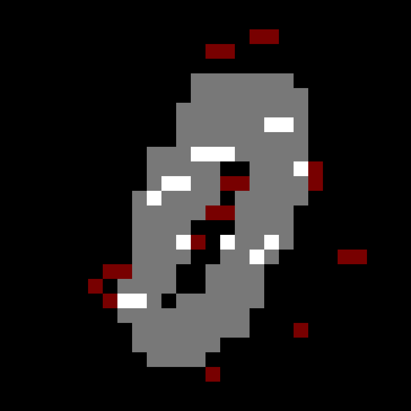
(a) SR found to explain $\mathcal{T}_{0}(\mathbf{e})$

(b) SR found to explain $\mathcal{T}_{1}(\mathbf{e})$

(c) SR found to explain $\mathcal{T}_{2}(\mathbf{e})$

(d) SR found to explain $\mathcal{T}_{3}(\mathbf{e})$

(e) SR found to explain $\mathcal{T}_{4}(\mathbf{e})$

(f) SR found to explain $\mathcal{T}_{5}(\mathbf{e})$

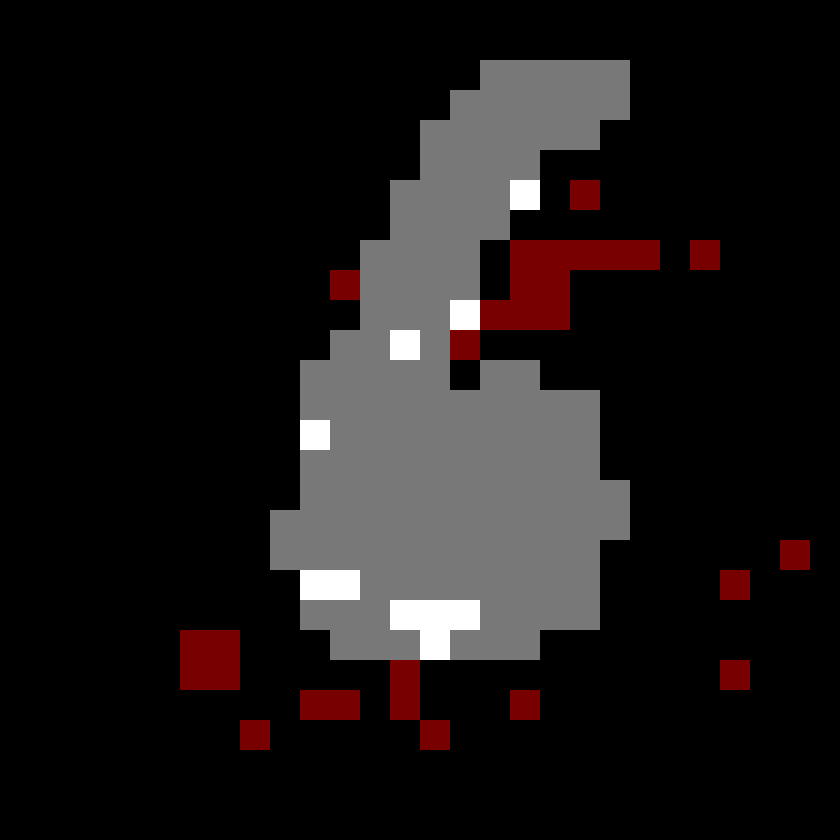
(g) SR found to explain $\mathcal{T}_{6}(\mathbf{e})$

(h) SR found to explain $\mathcal{T}_{7}(\mathbf{e})$

(i) SR found to explain $\mathcal{T}_{8}(\mathbf{e})$

(j) SR found to explain $\mathcal{T}_{9}(\mathbf{e})$

Figure 5: Visualization of SRs $\mathbf{e}^{\prime}$, with $|\mathbf{e}^{\prime}_{\bot}|\geq 730$, over positive instances $\mathbf{e}$.

(a) SR found to explain $\mathcal{T}_{0}(\mathbf{e})$

(b) SR found to explain $\mathcal{T}_{1}(\mathbf{e})$

(c) SR found to explain $\mathcal{T}_{2}(\mathbf{e})$

(d) SR found to explain $\mathcal{T}_{3}(\mathbf{e})$

(e) SR found to explain $\mathcal{T}_{4}(\mathbf{e})$

(f) SR found to explain $\mathcal{T}_{5}(\mathbf{e})$

(g) SR found to explain $\mathcal{T}_{6}(\mathbf{e})$

(h) SR found to explain $\mathcal{T}_{7}(\mathbf{e})$

(i) SR found to explain $\mathcal{T}_{8}(\mathbf{e})$

(j) SR found to explain $\mathcal{T}_{9}(\mathbf{e})$

Figure 6: Visualization of SRs $\mathbf{e}^{\prime}$, with $|\mathbf{e}^{\prime}_{\bot}|\geq 730$, over negative instances $\mathbf{e}$.

In the case of RFS, we did the same procedure to obtain the results illustrated in Figure 7. We choose 8 different positive instances for the digit 7 and used $\mathcal{T}_{7}$ to ask if exists a RFS with a certain amount of undefined features. We found a relevant feature set which explained all 8 positive results. The color coding is such that grey means irrelevant feature; in black and white we drew the original input on relevant features; and in green we represented the found RFS on the sub-figure at the center. An interesting observation based on Figure 5(h) is that pixels in both the southwest and southeast corners of the image are not relevant to the model’s decisions, which can be explained by the dataset’s absence of images of different classes that differ on said pixels.

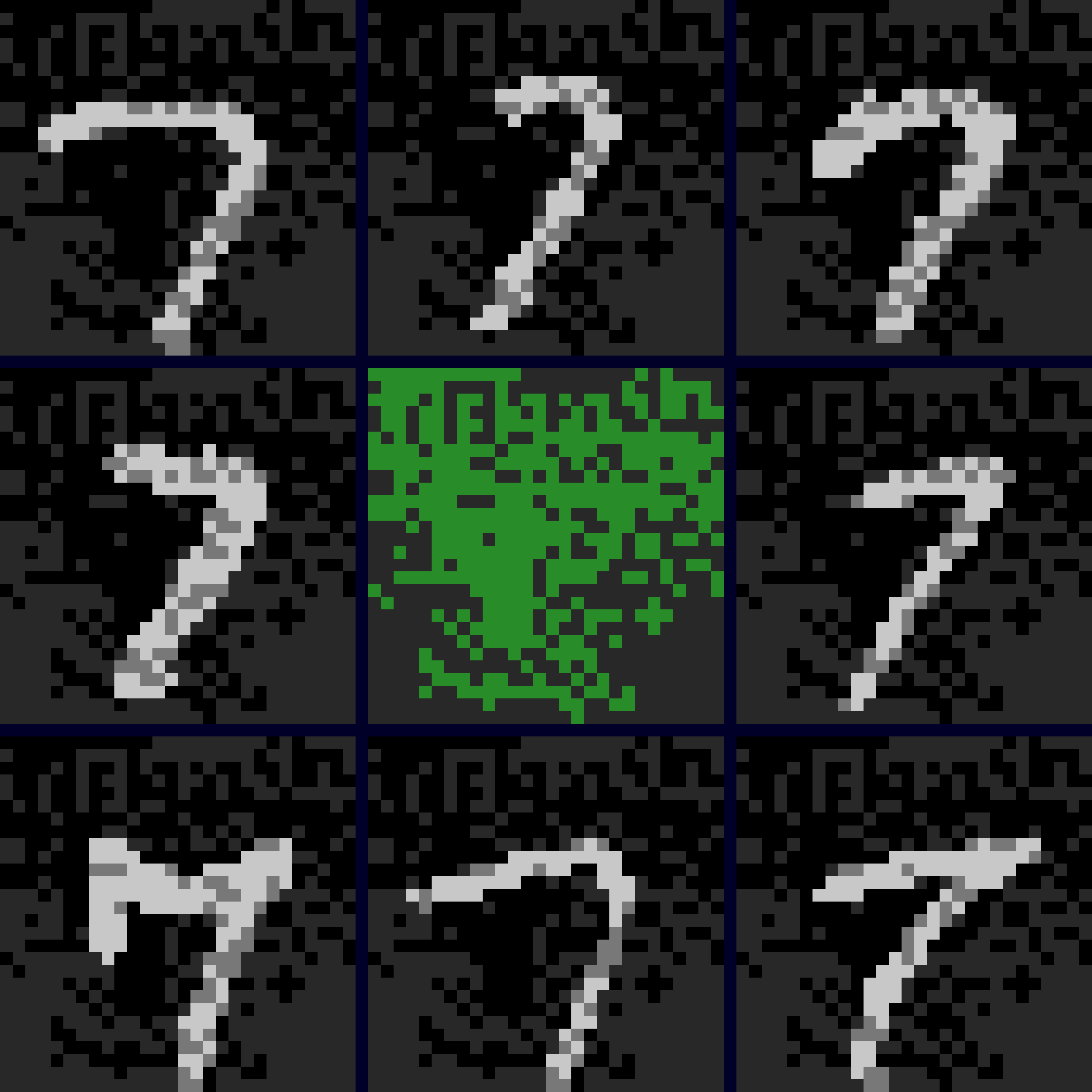
Figure 7: Visualization of RFS $\mathbf{e}^{\prime}$ over the 8 positive instances $\mathbf{e}_{i}$, such that $|\mathbf{e}^{\prime}_{\bot}|\geq 392$.

In order for ExplainDT to be usable in practice (e.g., by a data scientist), we must provide a high-level syntax in which queries are easier to write and interact with. While a more detailed description of the parsing is presented in Subsection A.2, Figure 8 presents an example interactive session with ExplainDT through its REPL interpreter.

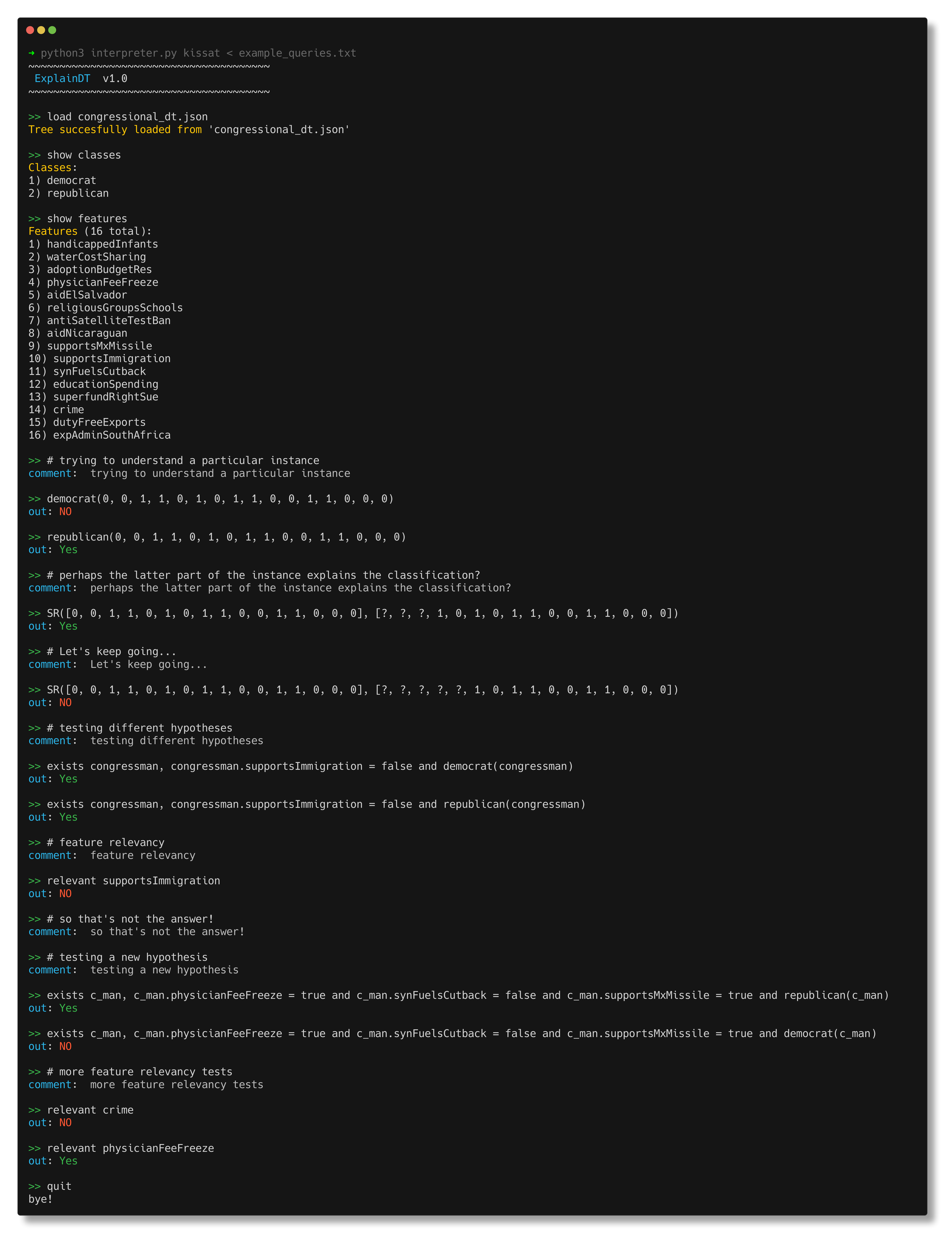
Figure 8: An interactive session using the ExplainDT REPL over the Congressional Voting Records Data Set [17].

More runtime plots and analysis.

Figure 4 show our time performance over the MNIST dataset. Finding small explanations is a particularly difficult task over high-dimensional datasets. In that sense, ExplainDT only takes seconds to find SRs over models up to 2500 nodes, which is much larger than the industry standard [37, 53]. Figure 9 shows how runtime scales for finding SRs over random decision trees, for dimensions up to $250$ and up to $2500$ nodes. Every datapoint consists of the average of $15$ different random instances to explain, and the candidate sufficient reasons are chosen to only have $5\%$ of their features undefined; this is because as the dataset is random, features are independent and also uncorrelated with the ground truth class, which suggests the absence of small SRs.

Figure 9: Evaluation time of the query $\exists y\,\textsc{SR}(x,y)$ with $|y_{\bot}|=0.05\times\dim(\mathcal{T})$, over synthetic random datasets.

Hardware.

All our experiments have been run on a personal computer with the following specifications: MacBook Pro (13-inch, M1, 2020), Apple M1 processor, 16 GB of RAM.

A.2 Detailed Implementation

Software Architecture.

Our code is written and tested in Python 3.10. Furthermore following libraries are required to build the project: pytest, argparse, pyparsing, scikit-learn, matplotlib, seaborn, pandas and typer. The input of our program consists of a Decision Tree model in a custom JSON structure and high-level queries against that model, which are provided by the user via the command line. The output is simply the truth value of the query provided by the user. As an intermediate step, the encoder generates a CNF file DIMACS format, a standard of common use in official SAT competitions. As a direct consequence, our implementation is solver-independent. Any solver whose input is a DIMACS CNF can be plugged into the application, including more performant future SAT solvers.

Regarding the software architecture, our object-oriented modularization is roughly segmented into 4 parts:

1. Parser and Interpreter: a method to get the user query parsing tree and generate a StratiFOILed query.

2. Context: all the model-based information to generate a CNF given a user query. E.g., Leaf, Tree, and Node classes, representing their respective objects in the decision tree.

3. Components: includes CNF, model partial instances and first-order logical connectives as Python classes. For example, the Not, And, and True classes. Also many useful StratiFOILed predicates are built as components. All components have simplify and encode methods, which are the implementation of the application Simplifier and Encoder respectively.

4. Experiments: a set of experiments that uses all the other modules to generate metrics and figures.

Parser and Interpreter.

This paragraph provides some detail into the main interface of ExplainDT: a REPL interpreter that users can directly interact with, writing queries in a high-level language. We use the Python library pyparsing, which offers high-level abstractions for parser combinators. In particular, a simplified version of the grammar we offer is the following:

constantvaltrue false 0 1 ?
constantconstantval constantval , constant
varname alphanumeric
varorconstconstant varname
classname alphanumeric
unarypredname full all_pos all_neg rfs classname
unarypred unarypredname( varorconst )
binarypredname subsumed by <= cons SR
binarypred biarypredname( varorconst, varorconst)
binaryconnective or and implies
qfree unarypred binarypred
not qfree qfree binaryconnective qfree
sentence qfree exists varname, sentence
for all varname, sentence
formula sentence not formula formula binaryconnective formula
modelfiname alphanumeric
action load modelfilename show features show classes
ExplainDT-expr action formula

The result of the parsing process is an abstract syntax tree, which a REPL interpreter executes. The interpreter distinguishes mainly between formulas (i.e., in StratiFOILed) and actions (e.g., load a different decision tree). While actions are completely executed by the interpreted, formulas are passed through the ${\color[rgb]{0,0,1}\text{Simplifier}}\to{\color[rgb]{0,0,1}\text{Encoder}}\to{\color[rgb]{0,0,1}\text{Solver}}$ pipeline.

Simplifier.

We implemented basic optimizations over the user queries, a very similar concept to the logical plan optimizer in a regular SQL database management system. As mentioned before, it is coded as a Component method.

Here we can distinguish two behaviors depending on the component type. In the case of first-order logical connectives, the simplify method propagates the simplification to their children checks if they are already truth values, and rewrites the plan. For example, if the child of the Not operator is False; then when the component simplification is finished, the parent of Not will have a True child during the calculation of its own simplification.

In the case of predicates, the simplify method performs optimizations over the generated circuits. When all the variables of a given predicate are constants, then the Simplifier calculates the truth value of the component. Notice that, this simplification is possible because it is a polynomial check of a formula with respect to the size of the model.

Encoder.

The encode method of each component builds the CNF of the subtree under the node that represents the component in the parsing tree. In other words, a logical connective like AND takes the CNF encoding of both its children and generates the CNF simply concatenating them. We tried to use libraries that had Tseitin transformation [52] over first-order formulas but none of them met our performance and correctness expectations, therefore we implemented our own version.

We distinguish between constants and variables. The encode method generates a different CNF depending on the representation used to indicate the semantics of a partial instance. For instance, $x\subseteq y$ has 3 circuits: one circuit when both $x$ and $y$ are variables, and two different circuits when only one of them is a constant. Notice that the case with two constants is resolved during the simplification phase.

It is worth noticing that a first-order logic formula $\varphi$ starting with a universal quantifier cannot directly be passed to a SAT-solver. Therefore, if a formula $\varphi$ is of the form $\varphi=\forall x\,P(x)$, then we apply the following identities:

$$\varphi:=\forall x\,P(x)=\neg\left(\neg\forall x\,P(x)\right)=\neg\left(\exists x\,\left(\neg P(x)\right)\right),$$

and thus it is enough to invert the truth value of the formula $\psi=\exists x\,\left(\neg P(x)\right)$, which is obtained with the aid of the SAT-solver.

Extended analysis on encoding size.

Illustrated in Table 6, we succeed in the generation of CNF formulas with a decent size, with respect to the query and the model. We attribute this result to two decisions we made about the Encoder. The first one was to study the first two layers of StratiFOILed and choose which predicates are useful to build more complex formulas. Then, to improve the performance, we though of the predicates as algorithms, circuits and finally as a CNF formula divided in ConsistencyCls and SemanticCls.

The second decision was to introduce new Boolean variables representing the predicates, i.e., a predicate variable is true if, and only if, the predicate is true. That representation allowed us to create our own efficient transform into CNF because logical connectives would now operate over singles variables instead of applying negation and distribution over considerably large circuits in CNF.

Limits of the implementation.

There is a countable number of predicates that can be included as circuits. We justify that the ones we choose are important based on the queries that are relevant according to the explainability literature. Nevertheless, more predicates can be easily added following the structure and object heritage.

Testing.

Our application has a high level of robustness regarding testing. Tests go from verifying the semantics of the vocabulary to checking the correctness of the circuits using handmade decision trees. The full suite of unit tests has 1182 individual tests.

A.3 Review of First-Order Logic

We review the definition of first-order logic (FO) over vocabularies consisting only of relations.

Syntax of FO.

A vocabulary $\sigma$ is a finite set $\{R_{1},\dots,R_{m}\}$, where each $R_{i}$ is a relation symbol with associated arity $n_{i}>0$, for $i\in\{1,\ldots,m\}$. We assume the existence of a countably infinite set of variables $\{x,y,z,\dots\}$, possibly with subscripts. The set of FO-formulas over $\sigma$ is inductively defined as follows.

1. If $x,y$ are variables, then $x=y$ is an ${\rm FO}$-formula over $\sigma$.

2. If relation symbol $R\in\sigma$ has arity $n>0$ and $x_{1},\dots,x_{n}$ are variables, then $R(x_{1},\dots,x_{n})$ is an ${\rm FO}$-formula over $\sigma$.

3. If $\varphi,\psi$ are ${\rm FO}$-formulas over $\sigma$, then $(\neg\varphi)$, $(\varphi\vee\psi)$, and $(\varphi\wedge\psi)$ are ${\rm FO}$-formulas over $\sigma$.

4. If $x$ is a variable and $\varphi$ is an ${\rm FO}$-formula over $\sigma$, then $(\exists x\,\varphi)$ and $(\forall x\,\varphi)$ are ${\rm FO}$-formulas over $\sigma$.

FO-formulas of type (1) and (2) are called atomic. A variable $x$ in ${\rm FO}$-formula $\varphi$ appears free, if there is an occurrence of $x$ in $\varphi$ that is not in the scope of a quantifier $\exists x$ or $\forall x$. An ${\rm FO}$-sentence is an ${\rm FO}$-formula without free variables. We often write $\varphi(x_{1},\ldots,x_{k})$ to denote that $\{x_{1},\ldots,x_{k}\}$ is the set of free variables of $\varphi$.

Semantics of FO.

${\rm FO}$-formulae over a vocabulary $\sigma$ are interpreted over $\sigma$-structures. Formally, a $\sigma$-structure is a tuple

$$\mathfrak{A} = \langle A,\,R_{1}^{\mathfrak{A}},\cdots,R_{m}^{\mathfrak{A}}\rangle,$$

where $A$ is the domain of $\mathfrak{A}$, and for each relation symbol $R\in\sigma$ of arity $n$, we have that $R^{\mathfrak{A}}$ is an $n$-ary relation over $A$. We call $R_{i}^{\mathfrak{A}}$ the interpretation of $R_{i}$ in $\mathfrak{A}$.

Let $\varphi$ be an ${\rm FO}$-formula over a vocabulary $\sigma$, and $\mathfrak{A}$ a $\sigma$-structure. Consider a mapping $\nu$ that associates an element in $A$ to each variable. We formally define the satisfaction of ${\rm FO}$-formula $\varphi$ over the pair $(\mathfrak{A},\nu)$, denoted by $(\mathfrak{A},\nu)\models\varphi$, as follows.

1. If $\varphi$ is an atomic formula of the form $x=y$, then $(\mathfrak{A},\nu)\models\varphi\,\Leftrightarrow\,\nu(t_{1})=\nu(t_{2})$.

2. If $\varphi$ is an atomic formula of the form $R(x_{1},\ldots,x_{n})$ for some $R\in\sigma$, then $(\mathfrak{A},\nu)\models\varphi\,\Leftrightarrow\,(\nu(x_{1}),\dots,\nu(x_{n}))\in R^{\mathfrak{A}}$.

3. If $\varphi$ is of the form $(\neg\psi)$, then $(\mathfrak{A},\nu)\models\varphi\,\Leftrightarrow\,(\mathfrak{A},\nu)\not\models\psi$.

4. If $\varphi$ is of the form $(\psi\vee\psi^{\prime})$, then $(\mathfrak{A},\nu)\models\varphi$ iff $(\mathfrak{A},\nu)\models\psi$ or $(\mathfrak{A},\nu)\models\psi^{\prime}$.

5. If $\varphi$ is of the form $(\psi\wedge\psi^{\prime})$, then $(\mathfrak{A},\nu)\models\varphi$ iff $(\mathfrak{A},\nu)\models\psi$ and $(\mathfrak{A},\nu)\models\psi^{\prime}$.

6. If $\varphi$ is of the form $(\exists x\,\psi)$, then $(\mathfrak{A},\nu)\models\varphi$ iff there exists $a\in A$ for which $(\mathfrak{A},\nu[x/a])\models\psi$. Here, $\nu[x/a]$ is a mapping that takes the same value as $\nu$ on every variable $y\neq x$, and takes value $a$ on $x$.

7. If $\varphi$ is of the form $(\forall x\,\psi)$, then $(\mathfrak{A},\nu)\models\varphi$ iff for every $a\in A$ we have that $(\mathfrak{A},\nu[x/a])\models\psi$.

For an FO-formula $\varphi(x_{1},\dots,x_{k})$ and assignment $\nu$ such that $\nu(x_{i})=a_{i}$, for each $i\in\{1,\ldots,k\}$, we write $\mathfrak{A}\models\varphi(a_{1},\ldots,a_{k})$ to denote that $(\mathfrak{A},\nu)\models\varphi$. If $\varphi$ is a sentence, we write simply $\mathfrak{A}\models\varphi$, as for any pair of mappings $\nu_{1}$, $\nu_{2}$ for the variables, it holds that $(\mathfrak{A},\nu_{1})\models\varphi$ iff $(\mathfrak{A},\nu_{2})\models\varphi$.

Games for FO distinguishability.

The quantifier rank of an ${\rm FO}$ formula $\phi$, denoted by ${\rm qr}(\phi)$, is the maximum depth of quantifier nesting in it. For $\mathfrak{A}$, we write ${\rm dom}(\mathfrak{A})$ to denote its domain.

Some proofs in this paper make use of Ehrenfeucht-Fraïssé  (EF) games. This game is played in two structures, $\mathfrak{A}_{1}$ and $\mathfrak{A}_{2}$, of the same schema, by two players, the spoiler and the duplicator. In round $i$ the spoiler selects a structure, say $\mathfrak{A}_{1}$, and an element $c_{i}$ in ${\rm dom}(\mathfrak{A}_{1})$; the duplicator responds by selecting an element $e_{i}$ in ${\rm dom}(\mathfrak{A}_{2})$. The duplicator wins in $k$ rounds, for $k\geq 0$, if $\{(c_{i},e_{i})\mid i\leq k\}$ defines a partial isomorphism between $\mathfrak{A}_{1}$ and $\mathfrak{A}_{2}$. If the duplicator wins no matter how the spoiler plays, we write $\mathfrak{A}_{1}\equiv_{k}\mathfrak{A}_{2}$. A classical result states that $\mathfrak{A}_{1}\equiv_{k}\mathfrak{A}_{2}$ iff $\mathfrak{A}_{1}$ and $\mathfrak{A}_{2}$ agree on all ${\rm FO}$ sentences of quantifier rank $\leq k$ (cf. [33]).

Also, if $\bar{a}$ is an $m$-tuple in ${\rm dom}(\mathfrak{A}_{1})$ and $\bar{b}$ is an $m$-tuple in ${\rm dom}(\mathfrak{A}_{2})$, where $m\geq 0$, we write $(\mathfrak{A}_{1},\bar{a})\equiv_{k}(\mathfrak{A}_{2},\bar{b})$ whenever the duplicator wins in $k$ rounds no matter how the spoiler plays, but starting from position $(\bar{a},\bar{b})$. In the same way, $(\mathfrak{A}_{1},\bar{a})\equiv_{k}(\mathfrak{A}_{2},\bar{b})$ iff for every ${\rm FO}$ formula $\phi(\bar{x})$ of quantifier rank $\leq k$, it holds that $\mathfrak{A}_{1}\models\phi(\bar{a})\Leftrightarrow\mathfrak{A}_{2}\models\phi(\bar{b})$.

It is well-known (cf. [33]) that there are only finitely many ${\rm FO}$ formulae of quantifier rank $k$, up to logical equivalence. The rank-$k$ type of an $m$-tuple $\bar{a}$ in a structure $\mathfrak{A}$ is the set of all formulae $\phi(\bar{x})$ of quantifier rank $\leq k$ such that $\mathfrak{A}\models\phi(\bar{a})$. Given the above, there are only finitely many rank-$k$ types, and each one of them is definable by an ${\rm FO}$ formula $\tau_{k}^{(\mathfrak{A},\bar{a})}(\bar{x})$ of quantifier rank $k$.

A.4 Definition of formula $\textsc{SUF}(x,y)$ in FOIL

Recall that $x\subsetneq y$ is a shorthand for the formula $x\subseteq y\wedge\neg(y\subseteq x)$. Then define the following auxiliary predicates:

$$L_{0}(x)\ =\ \forall y\,(x\subseteq y),$$

$$L_{1}(x)\ =\ \exists y\,(L_{0}(y)\wedge y\subsetneq x\wedge\neg\exists z\,(y\subsetneq z\wedge z\subsetneq x)),$$

$$\textsc{Opp}(x,y)\ =\ L_{1}(x)\wedge L_{1}(y)\wedge\neg\exists z\,(x\subseteq z\wedge y\subseteq z).$$

By using these predicates, we define a binary predicate SUF such that for every model $\mathcal{M}$ of dimension $n$ and every pair of partial instances $\mathbf{e}_{1},\mathbf{e}_{2}$ of dimension $n$, it holds that: $\mathcal{M}\models\textsc{SUF}(\mathbf{e},\mathbf{e}^{\prime})$ if and only if $\mathbf{e}_{\bot}=\mathbf{e}^{\prime}_{\bot}$. More precisely, we have that:

$$\textsc{SUF}(x,y)\ =\ \forall u\forall v\,( \textsc{Opp}(u,v)\ \to$$

$$[(u\subseteq x\wedge u\subseteq y\wedge\neg(v\subseteq x)\wedge\neg(v\subseteq y))\ \vee$$

$$\phantom{[}(v\subseteq x\wedge v\subseteq y\wedge\neg(u\subseteq x)\wedge\neg(u\subseteq y))\ \vee$$

$$\phantom{[}(u\subseteq x\wedge v\subseteq y\wedge\neg(u\subseteq y)\wedge\neg(v\subseteq x))\ \vee$$

$$\phantom{[}(u\subseteq y\wedge v\subseteq x\wedge\neg(u\subseteq x)\wedge\neg(v\subseteq y))\ \vee$$

$$\phantom{[}(\neg(u\subseteq x)\wedge\neg(u\subseteq y)\wedge\neg(v\subseteq x)\wedge\neg(v\subseteq y))]).$$

A.5 Proof of Theorem 1

The proof, which extends techniques from [33], requires introducing some terminology and establishing some intermediate lemmas.

Let $\mathcal{M}$, $\mathcal{M}^{\prime}$ be models of dimension $n$ and $p$, respectively, and consider the structures $\mathfrak{A}_{\mathcal{M}}=\langle\{0,1,\bot\}^{n},\subseteq^{\mathfrak{A}_{\mathcal{M}}},\textsc{Pos}^{\mathfrak{A}_{\mathcal{M}}}\rangle$ and $\mathfrak{A}_{\mathcal{M}^{\prime}}=\langle\{0,1,\bot\}^{p},\subseteq^{\mathfrak{A}_{\mathcal{M}^{\prime}}},\textsc{Pos}^{\mathfrak{A}_{\mathcal{M}^{\prime}}}\rangle$. We write $\mathfrak{A}_{\mathcal{M}}\oplus\mathfrak{A}_{\mathcal{M}^{\prime}}$ for the structure over the same vocabulary that satisfies the following:

• The domain of $\mathfrak{A}_{\mathcal{M}}\oplus\mathfrak{A}_{\mathcal{M}^{\prime}}$ is $\{0,1,\bot\}^{n+p}$.

• The interpretation of $\subseteq$ on $\mathfrak{A}_{\mathcal{M}}\oplus\mathfrak{A}_{\mathcal{M}^{\prime}}$ is the usual subsumption relation on $\{0,1,\bot\}^{n+p}$.

• The interpretation of Pos on $\mathfrak{A}_{\mathcal{M}}\oplus\mathfrak{A}_{\mathcal{M}^{\prime}}$ is the set of instances $\mathbf{e}\in\{0,1\}^{n+p}$ such that $(\mathbf{e}[1],\cdots,\mathbf{e}[n])\in\textsc{Pos}^{\mathfrak{A}_{\mathcal{M}}}$ or $(\mathbf{e}[n+1],\cdots,\mathbf{e}[n+p])\in\textsc{Pos}^{\mathfrak{A}_{\mathcal{M}^{\prime}}}$.

We start by establishing the following composition lemma.

Lemma 1.

Consider models $\mathcal{M}$, $\mathcal{M}_{1}$, and $\mathcal{M}_{2}$ of dimension $n$, $p$, and $q$, respectively, and assume that $(\mathfrak{A}_{\mathcal{M}_{1}},\{1\}^{p})\equiv_{k}(\mathfrak{A}_{\mathcal{M}_{2}},\{1\}^{q})$. Then it is the case that

$$\big{(}\mathfrak{A}_{\mathcal{M}}\oplus\mathfrak{A}_{\mathcal{M}_{1}},\{1\}^{n+p},\{\bot\}^{n}\times\{1\}^{p}\big{)}\,\equiv_{k}\,\big{(}\mathfrak{A}_{\mathcal{M}}\oplus\mathfrak{A}_{\mathcal{M}_{2}},\{1\}^{n+q},\{\bot\}^{n}\times\{1\}^{q}\big{)}.$$

Proof.

Let $\mathbf{e}_{i}$ and $\mathbf{e}^{\prime}_{i}$ be the moves played by Spoiler and Duplicator in $\mathfrak{A}_{\mathcal{M}}\oplus\mathfrak{A}_{\mathcal{M}_{1}}$ and $\mathfrak{A}_{\mathcal{M}}\oplus\mathfrak{A}_{\mathcal{M}_{2}}$, respectively, for the first $i\leq k$ rounds of the Ehrenfeucht-Fraïssé game

$$\big{(}\mathfrak{A}_{\mathcal{M}}\oplus\mathfrak{A}_{\mathcal{M}_{1}},\{1\}^{n+p},\{\bot\}^{n}\times\{1\}^{p}\big{)}\,\equiv_{k}\,\big{(}\mathfrak{A}_{\mathcal{M}}\oplus\mathfrak{A}_{\mathcal{M}_{2}},\{1\}^{n+q},\{\bot\}^{n}\times\{1\}^{q}\big{)}.$$

We write $\mathbf{e}_{i}=(\mathbf{e}_{i1},\mathbf{e}_{i2})$ to denote that $\mathbf{e}_{i1}$ is the tuple formed by the first $n$ features of $\mathbf{e}_{i}$ and $\mathbf{e}_{i2}$ is the one formed by the last $p$ features of $\mathbf{e}_{i}$. Similarly, we write $\mathbf{e}^{\prime}_{i}=(\mathbf{e}^{\prime}_{i1},\mathbf{e}^{\prime}_{i2})$ to denote that $\mathbf{e}^{\prime}_{i1}$ is the tuple formed by the first $n$ features of $\mathbf{e}^{\prime}_{i}$ and $\mathbf{e}^{\prime}_{i2}$ is the one formed by the last $q$ features of $\mathbf{e}^{\prime}_{i}$.

The winning strategy for Duplicator is as follows. Suppose $i-1$ rounds have been played, and for round $i$ the Spoiler picks element $\mathbf{e}_{i}\in\mathfrak{A}_{\mathcal{M}}\oplus\mathfrak{A}_{\mathcal{M}_{1}}$ (the case when he picks an element in $\mathfrak{A}_{\mathcal{M}}\oplus\mathfrak{A}_{\mathcal{M}_{2}}$ is symmetric). Assume also that $\mathbf{e}_{i}=(\mathbf{e}_{i1},\mathbf{e}_{i2})$. The duplicator then considers the position

$$\big{(}(\mathbf{e}_{12},\dots,\mathbf{e}_{(i-1)2}),(\mathbf{e}^{\prime}_{12},\dots,\mathbf{e}^{\prime}_{(i-1)2})\big{)}$$

on the game $(\mathfrak{A}_{\mathcal{M}_{1}},\{1\}^{p})\equiv_{k}(\mathfrak{A}_{\mathcal{M}_{2}},\{1\}^{q})$, and finds his response $\mathbf{e}^{\prime}_{i2}$ to $\mathbf{e}_{i2}$ in $\mathfrak{A}_{\mathcal{M}_{2}}$. The Duplicator then responds to the Spoiler’s move $\mathbf{e}_{i}\in\mathfrak{A}_{\mathcal{M}}\oplus\mathfrak{A}_{\mathcal{M}_{1}}$ by choosing the element $\mathbf{e}^{\prime}_{i}=(\mathbf{e}_{i1},\mathbf{e}^{\prime}_{i2})\in\mathfrak{A}_{\mathcal{M}}\oplus\mathfrak{A}_{\mathcal{M}_{2}}$.

Notice, by definition, that $\mathbf{e}_{i}=\{1\}^{n+p}$ iff $\mathbf{e}^{\prime}_{i}=\{1\}^{n+q}$. Similarly, $\mathbf{e}_{i}=\{\bot\}^{n}\times\{1\}^{p}$ iff $\mathbf{e}^{\prime}_{i}=\{\bot\}^{n}\times\{1\}^{q}$. Moreover, it is easy to see that playing in this way the Duplicator preserves the subsumption relation. Analogously, the strategy preserves the Pos relation. In fact, $\mathbf{e}_{i}$ is a positive instance of $\mathfrak{A}_{\mathcal{M}}\oplus\mathfrak{A}_{\mathcal{M}_{1}}$ iff $\mathbf{e}_{i1}$ is a positive instance of $\mathfrak{A}_{\mathcal{M}}$ or $\mathbf{e}_{i2}$ is a positive instance of $\mathfrak{A}_{\mathcal{M}_{1}}$. By definition, the latter follows if, and only if, $\mathbf{e}_{i1}$ is a positive instance of $\mathfrak{A}_{\mathcal{M}}$ or $\mathbf{e}^{\prime}_{i2}$ is a positive instance of $\mathfrak{A}_{\mathcal{M}_{2}}$, which in turn is equivalent to $\mathbf{e}^{\prime}_{i}$ being a positive instance of $\mathfrak{A}_{\mathcal{M}}\oplus\mathfrak{A}_{\mathcal{M}_{2}}$.

We conclude that this is a winning strategy for the Duplicator, and hence that

$$\big{(}\mathfrak{A}_{\mathcal{M}}\oplus\mathfrak{A}_{\mathcal{M}_{1}},\{1\}^{n+p},\{\bot\}^{n}\times\{1\}^{p}\big{)}\,\equiv_{k}\,\big{(}\mathfrak{A}_{\mathcal{M}}\oplus\mathfrak{A}_{\mathcal{M}_{2}},\{1\}^{n+q},\{\bot\}^{n}\times\{1\}^{q}\big{)}.$$

This finishes the proof of the lemma. ∎

We now consider structures of the form $\mathfrak{A}_{n}=\langle\{0,1,\bot\}^{n},\subseteq^{\mathfrak{A}}\rangle$, where $\subseteq$ is interpreted as the subsumption relation over $\{0,1,\bot\}^{n}$. For any such structure, we write $\mathfrak{A}_{n}^{+}$ for the structure over the vocabulary $\{\subseteq,\textsc{Pos}\}$ that extends $\mathfrak{A}$ by adding only the tuple $\{1\}^{n}$ to the interpretation of Pos. The following lemma is crucial for our proof.

Lemma 2.

If $n,p\geq 3^{k}$, then $\mathfrak{A}_{n}^{+}\equiv_{k}\mathfrak{A}_{p}^{+}$.

Proof.

We prove something slightly more general. For doing so, we need to define several concepts. Let $U=\{a_{i}\mid i>0\}$ be a countably infinite set. We take a disjoint copy $\overline{U}=\{\overline{a}_{i}\mid i>0\}$ of $U$. For an $X\subseteq U\cup\overline{U}$, we define

$$X_{U\setminus\overline{U}}\ :=\ \{a\in U\mid a\in X\text{ and }\overline{a}\not\in X\}$$

$$X_{U\cap\overline{U}}\ :=\ \{a\in U\mid a\in X\text{ and }\overline{a}\in X\}$$

$$X_{\overline{U}\setminus U}\ :=\ \{\overline{a}\in\overline{U}\mid\overline{a}\in X\text{ and }a\not\in X\}$$

The $\ell$-type of $X$, for $\ell\geq 0$, is the tuple

$$\big{(}\min{\{\ell,|X_{U\setminus\overline{U}}|\}},\,\min{\{\ell,|X_{U\cap\overline{U}}|\}},\,\min{\{\ell,|X_{\overline{U}\setminus U|}|\}}\big{)}.$$

We write $X\leftrightarrows_{\ell}X^{\prime}$, for $X,X^{\prime}\subseteq U\cup\overline{U}$, if $X$ and $X^{\prime}$ have the same $\ell$-type. If $X\subseteq U\cup\overline{U}$, then $X$ is well formed (wf) if for each $i>0$ at most one element from $\{a_{i},\overline{a}_{i}\}$ is in $X$.

We start with the following combinatorial lemma.

Lemma 3.

Assume that $X\leftrightarrows_{3^{k+1}}Y$, for $X,Y\subseteq U\cup\overline{U}$ and $k\geq 0$. Then:

• For every wf $X_{1}\subseteq X$, there exists a wf $Y_{1}\subseteq Y$ such that

  $$X_{1}\leftrightarrows_{3^{k}}Y_{1}\ \ \text{ and }\ \ X\setminus X_{1}\leftrightarrows_{3^{k}}Y\setminus Y_{1}.$$

• For every wf $Y_{1}\subseteq Y$, there exists a wf $X_{1}\subseteq X$ such that

  $$X_{1}\leftrightarrows_{3^{k}}Y_{1}\ \ \text{ and }\ \ X\setminus X_{1}\leftrightarrows_{3^{k}}Y\setminus Y_{1}.$$

Proof.

Given $Z\subseteq U$, we use $\overline{Z}$ to denote the set $\{\overline{a}\in\overline{U}\mid a\in Z\}$, and given $W\subseteq\overline{U}$, we use $\overline{W}$ to denote the set $\{a\in U\mid\overline{a}\in W\}$. Let $X_{1}$ be a wf subset of $X$. Then we have that $X_{1}=X_{1,1}\cup X_{1,2}\cup X_{1,3}\cup X_{1,4}$, where

$$X_{1,1} \subseteq X_{U\setminus\overline{U}},$$

$$X_{1,2} \subseteq \{a\in U\mid a\in X_{U\cap\overline{U}}\},$$

$$X_{1,3} \subseteq \{\overline{a}\in\overline{U}\mid a\in X_{U\cap\overline{U}}\},$$

$$X_{1,4} \subseteq X_{\overline{U}\setminus U},$$

and $\overline{X_{1,2}}\cap X_{1,3}=\emptyset$ (since $X$ is wf). We construct a set $Y_{1}=Y_{1,1}\cup Y_{1,2}\cup Y_{1,3}\cup Y_{1,4}$ by considering the following rules.

1. If $|X_{U\setminus\overline{U}}|<3^{k+1}$, then $|Y_{U\setminus\overline{U}}|=|X_{U\setminus\overline{U}}|$ since $X\leftrightarrows_{3^{k+1}}Y$. In this case, we choose $Y_{1,1}\subseteq Y_{U\setminus\overline{U}}$ in such a way that $|Y_{1,1}|=|X_{1,1}|$ and $|Y_{U\setminus\overline{U}}\setminus Y_{1,1}|=|X_{U\setminus\overline{U}}\setminus X_{1,1}|$.

   If $|X_{U\setminus\overline{U}}|\geq 3^{k+1}$, then $|Y_{U\setminus\overline{U}}|\geq 3^{k+1}$ since $X\leftrightarrows_{3^{k+1}}Y$. In this case, we choose $Y_{1,1}\subseteq Y_{U\setminus\overline{U}}$ in the following way. If $|X_{1,1}|<3^{k}$, then $|Y_{1,1}|=|X_{1,1}|$, and if $|X_{U\setminus\overline{U}}\setminus X_{1,1}|<3^{k}$, then $|Y_{U\setminus\overline{U}}\setminus Y_{1,1}|=|X_{U\setminus\overline{U}}\setminus X_{1,1}|$. Finally, if $|X_{1,1}|\geq 3^{k}$ and $|X_{U\setminus\overline{U}}\setminus X_{1,1}|\geq 3^{k}$, then $|Y_{1,1}|\geq 3^{k}$ and $|Y_{U\setminus\overline{U}}\setminus Y_{1,1}|\geq 3^{k}$. Notice that we can choose such a set $Y_{1,1}$ since $|Y_{U\setminus\overline{U}}|\geq 3^{k+1}$.

2. If $|X_{U\cap\overline{U}}|<3^{k+1}$, then $|Y_{U\cap\overline{U}}|=|X_{U\cap\overline{U}}|$ since $X\leftrightarrows_{3^{k+1}}Y$. In this case, we choose $Y_{1,2}\subseteq\{a\in U\mid a\in Y_{U\cap\overline{U}}\}$ and $Y_{1,3}\subseteq\{\overline{a}\in\overline{U}\mid a\in Y_{U\cap\overline{U}}\}$ in such a way that $\overline{Y_{1,2}}\cap Y_{1,3}=\emptyset$, $|Y_{1,2}|=|X_{1,2}|$, $|Y_{1,3}|=|X_{1,3}|$ and $|Y_{U\cap\overline{U}}\setminus(Y_{1,2}\cup\overline{Y_{1,3}})|=|X_{U\cap\overline{U}}\setminus(X_{1,2}\cup\overline{X_{1,3}})|$.

   If $|X_{U\cap\overline{U}}|\geq 3^{k+1}$, then $|Y_{U\cap\overline{U}}|\geq 3^{k+1}$ since $X\leftrightarrows_{3^{k+1}}Y$. In this case, we choose $Y_{1,2}\subseteq\{a\in U\mid a\in Y_{U\cap\overline{U}}\}$ and $Y_{1,3}\subseteq\{\overline{a}\in\overline{U}\mid a\in Y_{U\cap\overline{U}}\}$ in the following way.

   1. If $|X_{1,2}|<3^{k}$, $|X_{1,3}|<3^{k}$ and $|X_{U\cap\overline{U}}\setminus(X_{1,2}\cup\overline{X_{1,3}})|\geq 3^{k}$, then $|Y_{1,2}|=|X_{1,2}|$, $|Y_{1,3}|=|X_{1,3}|$ and $\overline{Y_{1,2}}\cap Y_{1,3}=\emptyset$. Notice that we can choose such sets $Y_{1,2}$ and $Y_{1,3}$ since $|Y_{\overline{U}\setminus U}|\geq 3^{k+1}$.

   2. If $|X_{1,2}|<3^{k}$, $|X_{1,3}|\geq 3^{k}$ and $|X_{U\cap\overline{U}}\setminus(X_{1,2}\cup\overline{X_{1,3}})|<3^{k}$, then $|Y_{1,2}|=|X_{1,2}|$, $|Y_{U\cap\overline{U}}\setminus(Y_{1,2}\cup\overline{Y_{1,3}})|=|X_{U\cap\overline{U}}\setminus(X_{1,2}\cup\overline{X_{1,3}})|$ and $\overline{Y_{1,2}}\cap Y_{1,3}=\emptyset$. Notice that we can choose such sets $Y_{1,2}$ and $Y_{1,3}$ since $|Y_{\overline{U}\setminus U}|\geq 3^{k+1}$.

   3. If $|X_{1,2}|\geq 3^{k}$, $|X_{1,3}|<3^{k}$ and $|X_{U\cap\overline{U}}\setminus(X_{1,2}\cup\overline{X_{1,3}})|<3^{k}$, then $|Y_{1,3}|=|X_{1,3}|$, $|Y_{U\cap\overline{U}}\setminus(Y_{1,2}\cup\overline{Y_{1,3}})|=|X_{U\cap\overline{U}}\setminus(X_{1,2}\cup\overline{X_{1,3}})|$ and $\overline{Y_{1,2}}\cap Y_{1,3}=\emptyset$. Notice that we can choose such sets $Y_{1,2}$ and $Y_{1,3}$ since $|Y_{\overline{U}\setminus U}|\geq 3^{k+1}$.

   4. If $|X_{1,2}|<3^{k}$, $|X_{1,3}|\geq 3^{k}$ and $|X_{U\cap\overline{U}}\setminus(X_{1,2}\cup\overline{X_{1,3}})|\geq 3^{k}$, then $|Y_{1,2}|=|X_{1,2}|$, $|Y_{1,3}|\geq 3^{k}$, $|Y_{U\cap\overline{U}}\setminus(Y_{1,2}\cup\overline{Y_{1,3}})|\geq 3^{k}$ and $\overline{Y_{1,2}}\cap Y_{1,3}=\emptyset$. Notice that we can choose such sets $Y_{1,2}$ and $Y_{1,3}$ since $|Y_{\overline{U}\setminus U}|\geq 3^{k+1}$.

   5. If $|X_{1,2}|\geq 3^{k}$, $|X_{1,3}|<3^{k}$ and $|X_{U\cap\overline{U}}\setminus(X_{1,2}\cup\overline{X_{1,3}})|\geq 3^{k}$, then $|Y_{1,3}|=|X_{1,3}|$, $|Y_{1,2}|\geq 3^{k}$, $|Y_{U\cap\overline{U}}\setminus(Y_{1,2}\cup\overline{Y_{1,3}})|\geq 3^{k}$ and $\overline{Y_{1,2}}\cap Y_{1,3}=\emptyset$. Notice that we can choose such sets $Y_{1,2}$ and $Y_{1,3}$ since $|Y_{\overline{U}\setminus U}|\geq 3^{k+1}$.

   6. If $|X_{1,2}|\geq 3^{k}$, $|X_{1,3}|\geq 3^{k}$ and $|X_{U\cap\overline{U}}\setminus(X_{1,2}\cup\overline{X_{1,3}})|<3^{k}$, then $|Y_{U\cap\overline{U}}\setminus(Y_{1,2}\cup\overline{Y_{1,3}})|=|X_{U\cap\overline{U}}\setminus(X_{1,2}\cup\overline{X_{1,3}})|$, $|Y_{1,2}|\geq 3^{k}$, $|Y_{1,3}|\geq 3^{k}$ and $\overline{Y_{1,2}}\cap Y_{1,3}=\emptyset$. Notice that we can choose such sets $Y_{1,2}$ and $Y_{1,3}$ since $|Y_{\overline{U}\setminus U}|\geq 3^{k+1}$.

   7. If $|X_{1,2}|\geq 3^{k}$, $|X_{1,3}|\geq 3^{k}$ and $|X_{U\cap\overline{U}}\setminus(X_{1,2}\cup\overline{X_{1,3}})|\geq 3^{k}$, then $|Y_{1,2}|\geq 3^{k}$, $|Y_{1,3}|\geq 3^{k}$, $|Y_{U\cap\overline{U}}\setminus(Y_{1,2}\cup\overline{Y_{1,3}})|\geq 3^{k}$ and $\overline{Y_{1,2}}\cap Y_{1,3}=\emptyset$. Notice that we can choose such sets $Y_{1,2}$ and $Y_{1,3}$ since $|Y_{\overline{U}\setminus U}|\geq 3^{k+1}$.

3. If $|X_{\overline{U}\setminus U}|<3^{k+1}$, then $|Y_{\overline{U}\setminus U}|=|X_{\overline{U}\setminus U}|$ since $X\leftrightarrows_{3^{k+1}}Y$. In this case, we choose $Y_{1,4}\subseteq Y_{\overline{U}\setminus U}$ in such a way that $|Y_{1,4}|=|X_{1,4}|$ and $|Y_{\overline{U}\setminus U}\setminus Y_{1,4}|=|X_{\overline{U}\setminus U}\setminus X_{1,4}|$.

   If $|X_{\overline{U}\setminus U}|\geq 3^{k+1}$, then $|Y_{\overline{U}\setminus U}|\geq 3^{k+1}$ since $X\leftrightarrows_{3^{k+1}}Y$. In this case, we choose $Y_{1,4}\subseteq Y_{\overline{U}\setminus U}$ in the following way. If $|X_{1,4}|<3^{k}$, then $|Y_{1,4}|=|X_{1,4}|$, and if $|X_{\overline{U}\setminus U}\setminus X_{1,4}|<3^{k}$, then $|Y_{\overline{U}\setminus U}\setminus Y_{1,4}|=|X_{\overline{U}\setminus U}\setminus X_{1,4}|$. Finally, if $|X_{1,4}|\geq 3^{k}$ and $|X_{\overline{U}\setminus U}\setminus X_{1,4}|\geq 3^{k}$, then $|Y_{1,4}|\geq 3^{k}$ and $|Y_{\overline{U}\setminus U}\setminus Y_{1,4}|\geq 3^{k}$. Notice that we can choose such a set $Y_{1,4}$ since $|Y_{\overline{U}\setminus U}|\geq 3^{k+1}$.

By definition of $Y_{1,1}$, $Y_{1,2}$, $Y_{1,3}$ and $Y_{1,4}$, it is straightforward to conclude that $Y_{1}$ is wf, $X_{1}\leftrightarrows_{3^{k}}Y_{1}$ and $(X\setminus X_{1})\leftrightarrows_{3^{k}}(Y\setminus Y_{1})$.

We have just proved that for every wf $X_{1}\subseteq X$, there exists a wf $Y_{1}\subseteq Y$ such that $X_{1}\leftrightarrows_{3^{k}}Y_{1}$ and $X\setminus X_{1}\leftrightarrows_{3^{k}}Y\setminus Y_{1}$. In the same way, it can be shown that for every wf $Y_{1}\subseteq Y$, there exists a wf $X_{1}\subseteq X$ such that $X_{1}\leftrightarrows_{3^{k}}Y_{1}$ and $X\setminus X_{1}\leftrightarrows_{3^{k}}Y\setminus Y_{1}$. This concludes the proof of the lemma.

∎

In the rest of the proof we make use of structures of the form $\mathfrak{A}^{*}=\langle 2^{X},\subseteq^{\mathfrak{A}^{*}}\rangle$, where $X\subseteq U\cup\overline{U}$ and $\subseteq^{\mathfrak{A}^{*}}$ is the relation that contains all pairs $(Y,Z)$, for $Y,Z\subseteq X$, such that $Y\subseteq Z$. Given two structures $\mathfrak{A}^{*}_{1}$ and $\mathfrak{A}^{*}_{2}$ of this form, perhaps with constants, we write $\mathfrak{A}^{*}_{1}\equiv_{k}^{{\rm wf}}\mathfrak{A}^{*}_{2}$ to denote that the Duplicator has a winning strategy in the $k$-round Ehrenfeucht-Fraïssé game played on structures $\mathfrak{A}^{*}_{1}$ and $\mathfrak{A}^{*}_{2}$, but where Spoiler and Duplicator are forced to play wf subsets of $U\cup\overline{U}$ only.

Consider structures $\mathfrak{A}^{*}_{1}=\langle 2^{X_{1}},\subseteq^{\mathfrak{A}^{*}_{1}}\rangle$ and $\mathfrak{A}^{*}_{2}=\langle 2^{X_{2}},\subseteq^{\mathfrak{A}^{*}_{2}}\rangle$ of the form described above. We claim that, for every $k\geq 0$,

$$X_{1}\leftrightarrows_{3^{k}}X_{2}\quad\Longrightarrow\quad\big{(}\mathfrak{A}^{*}_{1},(X_{1}\cap U)\big{)}\ \equiv_{k}^{{\rm wf}}\ \big{(}\mathfrak{A}^{*}_{2},(X_{2}\cap U)\big{)}.\quad\quad\quad(\dagger)$$

Before proving the claim in $(\dagger)$, we explain how it implies Lemma 2. Take a structure of the form $\mathfrak{A}_{n}=\langle\{0,1,\bot\}^{n},\subseteq^{\mathfrak{A}_{n}}\rangle$, where $\subseteq^{\mathfrak{A}_{n}}$ is the subsumption relation over $\{0,1,\bot\}^{n}$. Take, on the other hand, the structure $\mathfrak{A}_{n}^{*}=\langle 2^{X},\subseteq^{\mathfrak{A}_{n}^{*}}\rangle$, where $X=\{a_{1},\dots,a_{n},\bar{a}_{1},\dots,\bar{a}_{n}\}$. It can be seen that there is an isomorphism $f$ between $\mathfrak{A}_{n}$ and the substructure of $\mathfrak{A}_{n}^{*}$ induced by the wf subsets of $X$. The isomorphism $f$ takes an instance $\mathbf{e}\in\{0,1,\bot\}^{n}$ and maps it to $Y\subseteq X$ such that for every $i\in\{1,\dots,n\}$, (a) if $\mathbf{e}[i]=1$ then $a_{i}\in Y$, (b) if $\mathbf{e}[i]=0$ then $\bar{a}_{i}\in Y$, and (c) if $\mathbf{e}[i]=\bot$ then neither $a_{i}$ nor $\bar{a}_{i}$ is in $Y$. By definition, the isomorphism $f$ maps the tuple $\{1\}^{n}$ in $\mathfrak{A}_{n}$ to the set $X\cap U=\{a_{1},\dots,a_{n}\}$ in $\mathfrak{A}^{*}_{n}$.

From the claim in $(\dagger)$, it follows then that if $n,p\geq 3^{k}$ it is the case that

$$(\mathfrak{A}^{*}_{n},\{a_{1},\dots,a_{n}\})\ \equiv_{k}^{{\rm wf}}\ (\mathfrak{A}^{*}_{p},\{a_{1},\dots,a_{p}\}).$$

From our previous observations, this implies that

$$(\mathfrak{A}_{n},\{1\}^{n})\ \equiv_{k}\ (\mathfrak{A}_{p},\{1\}^{p}).$$

We conclude, in particular, that $\mathfrak{A}^{+}_{n}\equiv_{k}\mathfrak{A}^{+}_{p}$, as desired.

We now prove the claim in $(\dagger)$. We do it by induction on $k\geq 0$. The base cases $k=0,1$ are immediate. We now move to the induction case for $k+1$. Take structures $\mathfrak{A}^{*}_{1}=\langle 2^{X_{1}},\subseteq^{\mathfrak{A}^{*}_{1}}\rangle$ and $\mathfrak{A}^{*}_{2}=\langle 2^{X_{2}},\subseteq^{\mathfrak{A}^{*}_{2}}\rangle$ of the form described above, such that $X_{1}\leftrightarrows_{3^{k+1}}X_{2}$. Assume, without loss of generality, that for the first round the Spoiler picks the well formed element $X^{\prime}_{1}\subseteq X_{1}$ in the structure $\mathfrak{A}^{*}_{1}$. From Lemma 3, there exists $X^{\prime}_{2}\subseteq X_{2}$ such that

$$X^{\prime}_{1}\leftrightarrows_{3^{k}}X^{\prime}_{2}\ \ \text{ and }\ \ X_{1}\setminus X^{\prime}_{1}\leftrightarrows_{3^{k}}X_{2}\setminus X^{\prime}_{2}.$$

By induction hypothesis, the following holds:

$$\big{(}\langle 2^{X^{\prime}_{1}},\subseteq\rangle,(X^{\prime}_{1}\cap U)\big{)}\, \equiv^{\rm wf}_{k}\ \big{(}\langle 2^{X^{\prime}_{2}},\subseteq\rangle,(X^{\prime}_{2}\cap U)\big{)}$$

$$\big{(}\langle 2^{X_{1}\setminus X^{\prime}_{1}},\subseteq\rangle,((X_{1}\setminus X^{\prime}_{1})\cap U)\big{)}\, \equiv^{\rm wf}_{k}\ \big{(}\langle 2^{X_{2}\setminus X^{\prime}_{2}},\subseteq\rangle,((X_{2}\setminus X^{\prime}_{2})\cap U)\big{)}$$

A simple composition argument, similar to the one presented in Lemma 1, allows to obtain the following from these two expressions:

$$\big{(}\langle 2^{X_{1}},\subseteq\rangle,(X_{1}\cap U),X^{\prime}_{1}\big{)}\ \equiv_{k}^{{\rm wf}}\ \big{(}\langle 2^{X_{2}},\subseteq\rangle,(X_{2}\cap U),X^{\prime}_{2}\big{)}.$$ (3)

In particular, this holds because $X^{\prime}_{1}=(X_{1}\cap U)$ iff $X^{\prime}_{2}=(X_{2}\cap U)$. In fact, assume without loss of generality that $X^{\prime}_{1}=(X_{1}\cap U)$. In particular, $X^{\prime}_{1}\cap\overline{U}=\emptyset$, but then $X^{\prime}_{2}\cap\overline{U}=\emptyset$ since $X^{\prime}_{1}\leftrightarrows_{3^{k}}X^{\prime}_{2}$. It follows that $X^{\prime}_{2}=(X_{2}\cap U)$. But Equation (3) is equivalent with the following fact:

$$\big{(}\langle 2^{X_{1}},\subseteq\rangle,(X_{1}\cap U)\big{)}\ \equiv_{k+1}^{{\rm wf}}\ \big{(}\langle 2^{X_{2}},\subseteq\rangle,(X_{2}\cap U)\big{)}.$$

This finishes the proof of the lemma. ∎

We now proceed with the proof of Theorem 1. Assume, for the sake of contradiction, that there is in fact a formula $\textsc{MinimumSR}(x,y)$ in FOIL such that, for every decision tree $\mathcal{M}$, instance $\mathbf{e}$, and partial instance $\mathbf{e}^{\prime}$, we have that $\mathfrak{A}_{\mathcal{M}}\models\textsc{MinimumSR}(\mathbf{e},\mathbf{e}^{\prime})$ iff $\mathbf{e}^{\prime}$ is a minimum sufficient reason for $\mathbf{e}$ over $\mathcal{M}$. Let $k\geq 0$ be the quantifier rank of this formula. We show that there exist decision trees $\mathcal{M}_{1}$ and $\mathcal{M}_{2}$, instances $\mathbf{e}_{1}$ and $\mathbf{e}_{2}$ over $\mathcal{M}_{1}$ and $\mathcal{M}_{2}$, respectively, and partial instances $\mathbf{e}^{\prime}_{1}$ and $\mathbf{e}^{\prime}_{2}$ over $\mathcal{M}_{1}$ and $\mathcal{M}_{2}$, respectively, for which the following holds:

• $(\mathcal{M}_{1},\mathbf{e}_{1},\mathbf{e}^{\prime}_{1})\equiv_{k}(\mathcal{M}_{2},\mathbf{e}_{2},\mathbf{e}^{\prime}_{2})$, and hence

  $$\mathcal{M}_{1}\models\textsc{MinimumSR}(\mathbf{e}_{1},\mathbf{e}^{\prime}_{1})\ \Leftrightarrow\ \mathcal{M}_{2}\models\textsc{MinimumSR}(\mathbf{e}_{2},\mathbf{e}^{\prime}_{2}).$$

• It is the case that $\mathbf{e}^{\prime}_{1}$ is a minimum sufficient reason for $\mathbf{e}_{1}$ under $\mathcal{M}_{1}$, but $\mathbf{e}^{\prime}_{2}$ is not a minimum sufficient reason for $\mathbf{e}_{2}$ under $\mathcal{M}_{2}$.

This is our desired contradiction.

Let $\mathcal{M}_{n,p}$ be a decision tree of dimension $n+p$ such that, for every instance $\mathbf{e}\in\{0,1\}^{n+p}$, we have that $\mathcal{M}_{n,p}(\mathbf{e})=1$ iff $\mathbf{e}$ is of the form $\{1\}^{n}\times\{0,1\}^{p}$, i.e., the first $n$ features of $\mathbf{e}$ are set to 1, or $\mathbf{e}$ is of the form $\{0,1\}^{n}\times\{1\}^{p}$, i.e., the last $p$ features of $\mathbf{e}$ are set to 1. Take the instance $\mathbf{e}=\{1\}^{n+p}$. It is easy to see that $\mathbf{e}$ only has two minimal sufficient reasons in $\mathcal{M}_{n,p}$; namely, $\mathbf{e}_{1}=\{1\}^{n}\times\{\bot\}^{p}$ and $\mathbf{e}_{2}=\{\bot\}^{n}\times\{1\}^{p}$.

We define the following:

• $\mathcal{M}_{1}:=\mathcal{M}_{2^{k},2^{k}}$ and $\mathcal{M}_{2}:=\mathcal{M}_{2^{k},2^{k}+1}$.

• $\mathbf{e}_{1}:=\{1\}^{2^{k}+2^{k}}$ and $\mathbf{e}_{2}:=\{1\}^{2^{k}+2^{k}+1}$.

• $\mathbf{e}^{\prime}_{1}:=\{\bot\}^{2^{k}}\times\{1\}^{2^{k}}$ and $\mathbf{e}^{\prime}_{2}:=\{\bot\}^{2^{k}}\times\{1\}^{2^{k}+1}$.

From our previous observation, $\mathbf{e}^{\prime}_{1}$ is a minimal sufficient reason for $\mathbf{e}_{1}$ over $\mathcal{M}_{1}$ and $\mathbf{e}^{\prime}_{2}$ is a minimal sufficient reason for $\mathbf{e}_{2}$ over $\mathcal{M}_{2}$.

We show first that $(\mathcal{M}_{1},\mathbf{e}_{1},\mathbf{e}^{\prime}_{1})\equiv_{k}(\mathcal{M}_{2},\mathbf{e}_{2},\mathbf{e}^{\prime}_{2})$. It can be observed that $\mathfrak{A}_{\mathcal{M}_{1}}$ is of the form $\mathfrak{A}_{N}\oplus\mathfrak{A}_{N_{1}}$, where $N$ is a model of dimension $2^{k}$ that only accepts the tuple $\{1\}^{2^{k}}$ and the same holds for $N_{1}$. Analogously, $\mathfrak{A}_{\mathcal{M}_{2}}$ is of the form $\mathfrak{A}_{N}\oplus\mathfrak{A}_{N_{2}}$, where $N_{2}$ is a model of dimension $2^{k}+1$ that only accepts the tuple $\{1\}^{2^{k}+1}$. From Lemma 2, we have that $\mathfrak{A}_{N_{1}}\equiv_{k}\mathfrak{A}_{N_{2}}$. Notice that any winning strategy for the Duplicator on this game must map the tuples $\{1\}^{2^{k}}$ in $\mathfrak{A}_{N_{1}}$ and $\{1\}^{2^{k}+1}$ into each other. Therefore,

$$(\mathfrak{A}_{N_{1}},\{1\}^{2^{k}})\ \equiv_{k}\ (\mathfrak{A}_{N_{2}},\{1\}^{2^{k}+1}).$$

But then, from Lemma 1, we obtain that

$$\big{(}\mathfrak{A}_{N}\oplus\mathfrak{A}_{N_{1}},\{1\}^{2^{k}+2^{k}},\{\bot\}^{2^{k}}\times\{1\}^{2^{k}}\big{)}\ \equiv_{k}\ \big{(}\mathfrak{A}_{N}\oplus\mathfrak{A}_{N_{2}},\{1\}^{2^{k}+2^{k}+1},\{\bot\}^{2^{k}}\times\{1\}^{2^{k}+1}\big{)}.$$

We can then conclude that $(\mathcal{M}_{1},\mathbf{e}_{1},\mathbf{e}^{\prime}_{1})\equiv_{k}(\mathcal{M}_{2},\mathbf{e}_{2},\mathbf{e}^{\prime}_{2})$, as desired.

Notice now that $\mathbf{e}^{\prime}_{1}$ is a minimum sufficient reason for $\mathbf{e}_{1}$ over $\mathcal{M}_{1}$. In fact, by our previous observations, the only other minimal sufficient reason for $\mathbf{e}_{1}$ over $\mathcal{M}_{1}$ is $\mathbf{e}^{\prime\prime}_{1}=\{\bot\}^{2^{k}}\times\{1\}^{2^{k}}$, which has the same number of undefined features as $\mathbf{e}^{\prime}_{1}$. In turn, $\mathbf{e}^{\prime}_{2}$ is not a minimum sufficient reason for $\mathbf{e}_{2}$ over $\mathcal{M}_{2}$. This is because $\mathbf{e}^{\prime\prime}_{2}=\{\bot\}^{2^{k}+1}\times\{1\}^{2^{k}}$ is also a SR for $\mathbf{e}_{2}$ over $\mathcal{M}_{2}$, and $\mathbf{e}^{\prime\prime}_{2}$ has more undefined features than $\mathbf{e}^{\prime}_{2}$.

A.6 Definition of formula LEH in $\textsc{FOIL}^{+}$

Let GLB be the following formula:

$$\textsc{GLB}(x,y,z)\ =\ z\subseteq x\wedge z\subseteq y\wedge\forall w\,((w\subseteq x\wedge w\subseteq y)\to w\subseteq z).$$

Moreover, let LEH be a ternary predicate such that for every model $\mathcal{M}$ of dimension $n$ and every sequence of instances $\mathbf{e}_{1},\mathbf{e}_{2},\mathbf{e}_{3}$ of dimension $n$, it holds that: $\mathcal{M}\models\textsc{LEH}(\mathbf{e}_{1},\mathbf{e}_{2},\mathbf{e}_{3})$ if and only if the Hamming distance between $\mathbf{e}_{1}$ and $\mathbf{e}_{2}$ is less or equal than the Hamming distance between $\mathbf{e}_{1}$ and $\mathbf{e}_{3}$. Relation LEH can be expressed as follows in $\textsc{FOIL}^{+}$:

$$\textsc{LEH}(x,y,z)\ =\ \textsc{Full}(x)\wedge\textsc{Full}(y)\wedge\textsc{Full}(z)\ \wedge\\ \exists w_{1}\exists w_{2}\,(\textsc{GLB}(x,y,w_{1})\wedge\textsc{GLB}(x,z,w_{2})\wedge\textsc{LEL}(w_{2},w_{1})).$$

A.7 Proof of Theorem 2

For the first item, consider a fixed FOIL formula $\phi(x_{1},\dots,x_{m})$. We assume without loss of generality that $\phi$ is in prenex normal form, i.e., it is of the form

$$\exists\bar{y}_{1}\forall\bar{y}_{2}\cdots Q_{k}\bar{y}_{k}\,\psi(x_{1},\dots,x_{m},\bar{y}_{1},\dots,\bar{y}_{k}),\quad\quad(k\geq 0)$$

where $Q_{k}=\exists$ if $k$ is odd and $Q=\forall$ otherwise, and $\psi$ is a quantifier-free formula. An FOIL formula of this form is called a $\Sigma_{k}$-FOIL formula. Consider that $\mathcal{M}$ is a decision tree of dimension $n$, and assume that we want to check whether $\mathcal{M}\models\phi(\mathbf{e}_{1},\dots,\mathbf{e}_{m})$, for $\mathbf{e}_{1},\dots,\mathbf{e}_{m}$ given partial instances of dimension $n$. Since the formula $\phi$ is fixed, and thus the length of each tuple $\bar{y}_{i}$, for $i\leq k$, is constant, we can decide this problem in polynomial time by using a $\Sigma_{k}$-alternating Turing machine (as the fixed size quantifier-free formula $\psi$ can be evaluated in polynomial time over $\mathcal{M}$).

We now deal with the second item. We start by studying the complexity of the well-known quantified Boolean formula (QBF) problem for the case when the underlying formula (or, more precisely, the underlying Boolean function) is defined by a decision tree. More precisely, suppose that $\mathcal{M}$ is a decision tree over instances of dimension $n$. A $\Sigma_{k}$-QBF over $\mathcal{M}$, for $k>1$, is an expression

$$\exists P_{1}\forall P_{2}\cdots Q_{k}P_{k}\,\mathcal{M},$$

where $Q_{k}=\exists$ if $k$ is odd and $Q=\forall$ otherwise, and $P_{1},\dots,P_{k}$ is a partition of $\{1,\dots,n\}$ into $k$ equivalence classes. As an example, if $\mathcal{M}$ is of dimension 3 then $\exists\{2,1\}\forall\{3\}\,\mathcal{M}$ is a $\Sigma_{2}$-QBF over $\mathcal{M}$. The semantics of these expressions is standard. For instance, $\exists\{1,2\}\forall\{3\}\,\mathcal{M}$ holds if there exists a partial instance $(b_{1},b_{2},\bot)\in\{0,1\}\times\{0,1\}\times\{\bot\}$ such that both $\mathcal{M}(b_{1},b_{2},0)=1$ and $\mathcal{M}(b_{1},b_{2},1)=1$.

For a fixed $k>1$, we introduce then the problem $\Sigma_{k}$-QBF$(\mathsf{DTree})$. It takes as input a $\Sigma_{k}$-QBF $\alpha$ over $\mathcal{M}$, for $\mathcal{M}$ a decision tree, and asks whether $\alpha$ holds. We establish the following result, which we believe of independent interest, as (to the best of our knowledge) the complexity of the QBF problem over decision trees has not been studied in the literature.

Lemma 4.

For every even $k>1$, the problem $\Sigma_{k}$-QBF$(\mathsf{DTree})$ is $\Sigma_{k}^{\text{P}}$-complete.

Proof.

The upper bound is clear. For the lower bound we use a reduction from the following standard $\Sigma_{k}^{\text{P}}$-hard problem: Given a 3CNF formula $\varphi$ over set $X=\{x_{1},\dots,x_{m}\}$ of propositional variables, is it the case that the expression $\psi=\exists X_{1}\forall X_{2}\cdots\forall X_{k}\,\varphi$ holds, where $X_{1},\dots,X_{k}$ is a partition of $X$ in $k$ equivalence classes? From $\psi$ we build in polynomial time a $\Sigma_{k}$-QBF $\alpha$ over $\mathcal{M}_{\varphi}$, where $\mathcal{M}_{\varphi}$ is a decision tree that can be built in polynomial time from $\varphi$, such that

$$\text{$\psi$ holds}\quad\Longleftrightarrow\quad\text{$\alpha$ holds.}$$ (4)

We now explain how to define $\mathcal{M}_{\varphi}$ from the CNF formula $\varphi$. Let $\varphi=C_{1}\wedge\cdots\wedge C_{n}$ be a propositional formula, where each $C_{i}$ is a disjunction of three literals and does not contain repeated or complementary literals. Moreover, assume that $\{x_{1},\ldots,x_{m}\}$ is the set of variables occurring in $\varphi$, and the proof will use partial instances of dimension $n+m$. Notice that the last $m$ features of such a partial instance $\mathbf{e}$ naturally define a truth assignment for the propositional formula $\varphi$. More precisely, for every $i\in\{1,\ldots,n\}$, we use notation $\mathbf{e}(C_{i})=1$ to indicate that there is a disjunct $\ell$ of $C_{i}$ such that $\ell=x_{j}$ and $\mathbf{e}[n+j]=1$, or $\ell=\neg x_{j}$ and $\mathbf{e}[n+j]=0$, for some $j\in\{1,\ldots,m\}$. Furthermore, we write $\mathbf{e}(\varphi)=1$ if $\mathbf{e}(C_{i})=1$ for every $i\in\{1,\ldots,n\}$.

For each clause $C_{i}$ ($i\in\{1,\ldots,n\}$), let $\mathcal{M}_{C_{i}}$ be a decision tree of dimension $n+m$ (but that will only use features $n+1,\ldots,n+m$) such that for every entity $\mathbf{e}$: $\mathcal{M}_{C_{i}}(\mathbf{e})=1$ if and only $\mathbf{e}(C_{i})=1$. Notice that $\mathcal{M}_{C_{i}}$ can be constructed in constant time as it only needs to contain at most eight paths of depth 3. For example, assuming that $C=(x_{1}\vee x_{2}\vee x_{3})$, a possible decision tree $\mathcal{M}_{C}$ is depicted in the following figure:

Moreover, define $\mathcal{M}_{\varphi}$ as the following decision tree.

Recall that the set of features of $\mathcal{M}_{\varphi}$ is $[1,n+m]$. The formula $\alpha$ is defined as

$$\exists P_{1}\forall P_{2}\cdots\forall(P_{k}\cup P)\,\mathcal{M}_{\varphi},$$

assuming that $P_{i}$, for $1\leq i\leq k$, is the set $\{n+\ell\mid x_{\ell}\in X_{i}\}$, and $P=\{1,\dots,n\}$. That is, $P_{i}$ is the set of features from $\mathcal{M}_{\varphi}$ that represent the variables in $X_{i}$ and $P$ is the set of features that are used to encode the clauses of $\varphi$.

We show next that the equivalence stated in (4) holds. For simplicity, we only do it for the case $k=2$. The proof for $k>2$ uses exactly the same ideas, only that it is slightly more cumbersome.

Assume, on the one hand, that $\psi=\exists X_{1}\forall X_{2}\varphi$ holds. That is, there exists an assignment $\sigma_{1}:X_{1}\to\{0,1\}$ such that for every assignment $\sigma_{2}:X_{2}\to\{0,1\}$, it is the case that $\varphi$ holds when variables in $X_{1}$ are interpreted according to $\sigma_{1}$ and variables in $X_{2}$ according to $\sigma_{2}$. We show next that $\alpha=\exists P_{1}\forall(P_{2}\cup P)\mathcal{M}_{\varphi}$ holds, where $P_{1}$, $P_{2}$, and $P$ are defined as above. Take the partial instance $\mathbf{e}_{\sigma_{1}}$ of dimension $n+m$ that naturally “represents” the assignment $\sigma_{1}$; that is:

• $\mathbf{e}_{\sigma_{1}}[i]=\bot$, for each $i\in\{1,\dots,n\}$,

• $\mathbf{e}_{\sigma_{1}}[n+i]=\sigma_{1}(x_{i})$, for each $i\in\{1,\dots,m\}$ with $x_{i}\in X_{1}$, and

• $\mathbf{e}_{\sigma_{1}}[n+i]=\bot$, for each $i\in\{1,\dots,m\}$ with $x_{i}\not\in X_{1}$.

To show that $\alpha$ holds, it suffices to show that $\mathcal{M}_{\varphi}(\mathbf{e})=1$ for every instance $\mathbf{e}$ of dimension $n+m$ that subsumes $\mathbf{e}_{\sigma_{1}}$. Take an arbitrary such an instance $\mathbf{e}\in\{0,1\}^{n+m}$. Notice that if $\mathbf{e}[i]=1$, for every $i\in\{1,\dots,n\}$, then $\mathcal{M}_{\varphi}(\mathbf{e})=1$ by definition of $\mathcal{M}_{\varphi}$. Suppose then that there exists a minimum value $i\in\{1,\dots,n\}$ such that $\mathbf{e}[i]=0$. Hence, to show that $\mathcal{M}_{\varphi}(\mathbf{e})=1$ we need to show that $\mathcal{M}_{C_{i}}(\mathbf{e})=1$. But this follows easily from the fact that $\mathbf{e}$ naturally represents an assignment $\sigma$ for $\varphi$ such that the restriction of $\sigma$ to $X_{1}$ is precisely $\sigma_{1}$. We know that any such an assignment $\sigma$ satisfies $\varphi$, and therefore it satisfies $C_{i}$. It follows that $\mathcal{M}_{C_{i}}(\mathbf{e})=1$.

Assume, on the other hand, that $\alpha=\exists P_{1}\forall(P_{2}\cup P)\mathcal{M}_{\varphi}$ holds. Then there exists a partial instance $\mathbf{e}$ such that the following statements hold:

• $\mathbf{e}[i]\neq\bot$ iff for some $j\in\{1,\dots,m\}$ it is the case that $i=n+j$ and $j\in P_{1}$, and

• for every completion $\mathbf{e}^{\prime}$ of $\mathbf{e}$ we have that $\mathcal{M}_{\varphi}(\mathbf{e})=1$.

We show next that $\psi=\exists X_{1}\forall X_{2}\varphi$ holds. Let $\sigma_{1}:X_{1}\to\{0,1\}$ be the assignment for the variables in $X_{1}$ that is naturally defined by $\mathbf{e}$. Take an arbitrary assignment $\sigma_{2}:X_{2}\to\{0,1\}$. It suffices to show that each clause $C_{i}$ of $\varphi$, for $i\in\{1,\dots,n\}$, is satisfied by the assignment that interprets the variables in $X_{1}$ according to $\sigma_{1}$ and the variables in $\sigma_{2}$ according to $X_{2}$. Let us define a completion $\mathbf{e}^{\prime}$ of $\mathbf{e}$ that satisfies the following:

• $\mathbf{e}^{\prime}[i]=0$,

• $\mathbf{e}^{\prime}[j]=1$, for each $j\in\{1,\dots,n\}$ with $i\neq j$,

• $\mathbf{e}^{\prime}[n+j]=\sigma_{1}(x_{j})$, if $j\in\{1,\dots,m\}$ and $x_{j}\in P_{1}$, and

• $\mathbf{e}^{\prime}[n+j]=\sigma_{2}(x_{j})$, if $j\in\{1,\dots,m\}$ and $x_{j}\in P_{2}$.

We know that $\mathcal{M}_{\varphi}(\mathbf{e}^{\prime})=1$, which implies that $\mathcal{M}_{C_{i}}(\mathbf{e}^{\prime})=1$ (since $\mathbf{e}^{\prime}$ takes value 0 for feature $i$). We conclude that $C_{i}$ is satisfied by the assignment which is naturally defined by $\mathbf{e}^{\prime}$, which is precisely the one that interprets the variables in $X_{1}$ according to $\sigma_{1}$ and the variables in $\sigma_{2}$ according to $X_{2}$. ∎

With the help of Lemma 4 we can now finish the proof of the theorem. We reduce from $\Sigma_{k}$-QBF$(\mathsf{DTree})$. The input to $\Sigma_{k}$-QBF$(\mathsf{DTree})$ is given by an expression $\alpha$ of the form

$$\exists P_{1}\forall P_{2}\cdots\forall_{k}P_{k}\,\mathcal{M},$$

for $\mathcal{M}$ a decision tree of dimension $n$ and $P_{1},\dots,P_{k}$ a partition of $\{1,\dots,n\}$. We explain next how the formula $\phi_{k}(x_{1},\dots,x_{k})$ is defined.

We start by defining some auxiliary terminology. We use $x[i]$ to denote the $i$-th feature of the partial instance that is assigned to variable $x$. We define the following formulas.

• ${\sf Undef}(x):=\neg\exists y(y\subset x)$. That is, ${\sf Undef}$ defines the set that only consists of the partial instance $\{\bot\}^{n}$ in which all components are undefined.

• ${\sf Single}(x):=\exists y(y\subset x)\wedge\forall y(y\subset x\,\rightarrow\,{\sf Undef}(y))$. That is, ${\sf Single}$ defines the set that consists precisely of those partial instances in $\{0,1,\bot\}^{n}$ which have at most one component that is defined.

• $(x\sqcup y=z):=(x\subseteq z)\wedge(y\subseteq z)\wedge\neg\exists w\big{(}(x\subseteq w)\wedge(y\subseteq w)\wedge(w\subset z)\big{)}$. That is, $z$, if it exists, is the join of $x$ and $y$. In other words, $z$ is defined if every feature that is defined over $x$ and $y$ takes the same value in both partial instances, and, in such case, for each $1\leq i\leq n$ we have that $z[i]=x[i]\sqcup y[i]$, where $\sqcup$ is the commutative and idempotent binary operation that satisfies $\bot\sqcup 0=0$ and $\bot\sqcup 1=1$.

  As an example, $(1,0,\bot,\bot)\sqcup(1,\bot,\bot,1)=(1,0,\bot,1)$, while $(1,\bot)\sqcup(0,0)$ is undefined.

• $(x\sqcap y=z):=(z\subseteq x)\wedge(z\subseteq y)\wedge\neg\exists w\big{(}(w\subseteq x)\wedge(w\subseteq y)\wedge(z\subset w)\big{)}$. That is, $z$ is the meet of $x$ and $y$ (which always exists). In other words, for each $1\leq i\leq n$ we have that $z[i]=x[i]\sqcap y[i]$, where $\sqcap$ is the commutative and idempotent binary operation that satisfies $\bot\sqcap 0=\bot\sqcap 1=0\sqcap 1=\bot$.

  As an example, $(1,0,\bot,\bot)\sqcap(1,\bot,\bot,1)=(1,\bot,\bot,\bot)$, while $(1,\bot)\sqcap(0,0)=(\bot,\bot)$.

• ${\sf Comp}(x,y):=\exists w\exists z({\sf Undef}(z)\,\wedge\,x\sqcup y=w\,\wedge\,x\sqcap y=z)$. That is, ${\sf Comp}$ defines the pairs $(\mathbf{e}_{1},\mathbf{e}_{2})$ of partial instances in $\{0,1,\bot\}^{n}\times\{0,1,\bot\}^{n}$ such that no feature that is defined in $\mathbf{e}_{1}$ is also defined in $\mathbf{e}_{2}$, and vice versa. In fact, assume for the sake of contradiction that this is not the case. By symmetry, we only have to consider the following two cases.

  • There is an $i\leq n$ with $\mathbf{e}_{1}[i]=1$ and $\mathbf{e}_{2}[i]=0$. Then the join of $\mathbf{e}_{1}$ and $\mathbf{e}_{2}$ does not exist.

  • There is an $i\leq n$ with $\mathbf{e}_{1}[i]=\mathbf{e}_{2}[i]=1$. Then the $i$-th component of the meet of $\mathbf{e}_{1}$ and $\mathbf{e}_{2}$ takes value 1, and hence $\mathbf{e}_{1}\sqcap\mathbf{e}_{2}\neq\{\bot\}^{n}$.

• ${\sf MaxComp}(x,y):={\sf Comp}(x,y)\,\wedge\,\neg\exists z\big{(}(y\subset z)\wedge{\sf Comp}(x,z)\big{)}$. That is, ${\sf MaxComp}$ defines the pairs $(\mathbf{e}_{1},\mathbf{e}_{2})$ such that the components that are defined in $\mathbf{e}_{1}$ are precisely the ones that are undefined in $\mathbf{e}_{2}$, and vice versa.

• ${\sf Rel}(x,y):=\neg\exists z\big{(}(z\subseteq y)\,\wedge\,{\sf Single}(z)\,\wedge\,{\sf Comp}(x,z)\big{)}$. That is, ${\sf Rel}$ defines the pairs $(\mathbf{e}_{1},\mathbf{e}_{2})$ of partial instances in $\{0,1,\bot\}^{n}\times\{0,1,\bot\}^{n}$ such that every feature that is defined in $\mathbf{e}_{1}$ is also defined in $\mathbf{e}_{2}$.

• ${\sf MaxRel}(x,y):={\sf Rel}(x,y)\,\wedge\,\neg\exists z\big{(}(y\subset z)\wedge{\sf Rel}(x,z)\big{)}$. That is, ${\sf MaxRel}$ defines the pairs $(\mathbf{e}_{1},\mathbf{e}_{2})$ such that the features defined in $\mathbf{e}_{1}$ and in $\mathbf{e}_{2}$ are the same.

We now define the formula $\phi_{k}(x_{1},\dots,x_{k})$ as

$$\exists y_{1}\forall y_{2}\cdots\forall y_{k}\,\bigg{(}\bigwedge_{i=1}^{k}{\sf MaxRel}(x_{i},y_{i})\,\wedge\,\forall z\big{(}z=y_{1}\sqcup y_{2}\sqcup\cdots\sqcup y_{k}\,\rightarrow\,\textsc{Pos}(z)\big{)}\bigg{)}.$$

For each $i$ with $1\leq i\leq k$, let $\mathbf{e}_{i}$ be the partial instance of dimension $n$ such that

$$\mathbf{e}_{i}[j]\ =\ \begin{cases}1\quad\quad&\text{if $j\in P_{i}$,}\\ \bot&\text{otherwise.}\end{cases}$$

That is, $\mathbf{e}_{i}$ takes value 1 over the features in $P_{i}$ and it is undefined over all other features. We claim that $\alpha$ holds if, and only if, $\mathcal{M}\models\phi_{k}(\mathbf{e}_{1},\dots,\mathbf{e}_{k})$. The result then follows since $\mathcal{M}$ is a decision tree.

For the sake of presentation we only prove the aforementioned equivalence for the case when $k=2$, since the extension to $k>2$ is standard (but cumbersome). That is, we consider the case when $\alpha=\exists P_{1}\forall P_{2}\mathcal{M}$ and, therefore,

$$\phi_{2}(x_{1},x_{2})=\exists y_{1}\forall y_{2}\,\bigg{(}{\sf MaxRel}(x_{1},y_{1})\,\wedge\,{\sf MaxRel}(x_{2},y_{2})\,\wedge\,\forall z\big{(}z=y_{1}\sqcup y_{2}\,\rightarrow\,\textsc{Pos}(z)\big{)}\bigg{)}.$$

• Assume first that $\mathcal{M}\models\phi_{2}(\mathbf{e}_{1},\mathbf{e}_{2})$. Hence, there exists a partial instance $\mathbf{e}^{\prime}_{1}$ such that

  $$\mathcal{M}\,\models\,\forall y_{2}\,\bigg{(}{\sf MaxRel}(\mathbf{e}_{1},\mathbf{e}^{\prime}_{1})\,\wedge\,{\sf MaxRel}(\mathbf{e}_{2},y_{2})\,\wedge\,\forall z\big{(}z=\mathbf{e}^{\prime}_{1}\sqcup y_{2}\,\rightarrow\,\textsc{Pos}(z)\big{)}\bigg{)}.$$

  This means that the features defined in $\mathbf{e}_{1}$ and $\mathbf{e}^{\prime}_{1}$ are exactly the same, and hence $\mathbf{e}^{\prime}_{1}$ is a partial instance that is defined precisely over the features in $P_{1}$. We claim that every instance $\mathbf{e}$ that is a completion of $\mathbf{e}^{\prime}_{1}$ satisfies $\mathcal{M}(\mathbf{e})=1$, thus showing that $\alpha$ holds. In fact, take an arbitrary such a completion $\mathbf{e}$. By definition, $\mathbf{e}$ can be written as $\mathbf{e}^{\prime}_{1}\sqcup\mathbf{e}^{\prime}_{2}$, where $\mathbf{e}^{\prime}_{2}$ is a partial instance that is defined precisely over those features not in $P_{1}$, i.e., over the features in $P_{2}$. Thus,

  $$\mathcal{M}\,\models\,{\sf MaxRel}(\mathbf{e}_{1},\mathbf{e}^{\prime}_{1})\,\wedge\,{\sf MaxRel}(\mathbf{e}_{2},\mathbf{e}^{\prime}_{2})\,\wedge\,\mathbf{e}=\mathbf{e}^{\prime}_{1}\sqcup\mathbf{e}^{\prime}_{2},$$

  which allows us to conclude that $\mathcal{M}\models\textsc{Pos}(\mathbf{e})$. This tells us that $\mathcal{M}(\mathbf{e})=1$.

• Assume in turn that $\alpha$ holds, and hence that there is a partial instance $\mathbf{e}^{\prime}_{1}$ that is defined precisely over the features in $P_{1}$ such that that every instance $\mathbf{e}$ that is a completion of $\mathbf{e}^{\prime}_{1}$ satisfies $\mathcal{M}(\mathbf{e})=1$. We claim that

  $$\mathcal{M}\,\models\,\forall y_{2}\,\bigg{(}{\sf MaxRel}(\mathbf{e}_{1},\mathbf{e}^{\prime}_{1})\,\wedge\,{\sf MaxRel}(\mathbf{e}_{2},y_{2})\,\wedge\,\forall z\big{(}z=\mathbf{e}^{\prime}_{1}\sqcup y_{2}\,\rightarrow\,\textsc{Pos}(z)\big{)}\bigg{)},$$

  which implies that $\mathcal{M}\models\phi_{2}(\mathbf{e}_{1},\mathbf{e}_{2})$. In fact, let $\mathbf{e}^{\prime}_{2}$ be an arbitrary instance such that ${\sf MaxRel}(\mathbf{e}_{2},\mathbf{e}^{\prime}_{2})$ holds. By definition, $\mathbf{e}^{\prime}_{2}$ is defined precisely over the features in $P_{2}$. Let $\mathbf{e}=\mathbf{e}^{\prime}_{1}\sqcup\mathbf{e}^{\prime}_{2}$. Notice that $\mathbf{e}$ is well-defined since the sets of features defined in $\mathbf{e}^{\prime}_{1}$ and $\mathbf{e}^{\prime}_{2}$, respectively, are disjoint. Moreover, $\mathbf{e}$ is a completion of $\mathbf{e}^{\prime}_{1}$ as $P_{1}\cup P_{2}=\{1,\dots,n\}$. We then have that $\mathcal{M}(\mathbf{e})=1$ as $\alpha$ holds. This allows us to conclude that $\mathcal{M}\models\textsc{Pos}(\mathbf{e})$, and hence that $\mathcal{M}\models\phi_{2}(\mathbf{e}_{1},\mathbf{e}_{2})$.

This concludes the proof of the theorem.

A.8 $\subseteq$ and LEL cannot be defined in terms of each other

First, we show that predicate LEL cannot be defined in terms of predicate $\subseteq$.

Lemma 5.

There is no formula $\textsc{LEL}(x,y)$ in $\textsc{FOIL}^{+}$ defined over the vocabulary $\{\subseteq\}$ such that, for every decision tree $\mathcal{T}$ and pair of partial instances $\mathbf{e}$, $\mathbf{e}^{\prime}$, we have that

$$\mathcal{T}\models\textsc{LEL}(\mathbf{e},\mathbf{e}^{\prime})\ \Longleftrightarrow\ |\mathbf{e}_{\bot}|\geq|\mathbf{e}^{\prime}_{\bot}|.$$

Proof.

For the sake of contradiction, assume that $\textsc{LEL}(x,y)$ is definable in $\textsc{FOIL}^{+}$ over the vocabulary $\{\subseteq\}$. Then the following are formulas in FOIL:

$$\textsc{SR}(x,y) = \textsc{Full}(x)\wedge\,y\subseteq x\,\wedge\,\forall z\,\big{(}y\subseteq z\wedge\textsc{Full}(z)\,\rightarrow\,(\textsc{Pos}(z)\leftrightarrow\textsc{Pos}(\ x))\big{)},$$

$$\textsc{MinimumSR}(x,y) = \textsc{SR}(x,y)\wedge\forall z\big{(}\textsc{SR}(x,z)\to(\textsc{LEL}(z,y)\to\textsc{LEL}(y,z))\big{)}.$$

But the second formula verifies if a partial instance $x$ is a minimum SR for a given instance $y$, which contradicts the inexpressibility result of Theorem 1, and hence concludes the proof of the lemma. ∎

Second, we show that predicate $\subseteq$ cannot be defined in terms of predicate LEL.

Lemma 6.

There is no formula $\textsc{Subsumed}(x,y)$ in $\textsc{FOIL}^{+}$ defined over the vocabulary $\{\textsc{LEL}\}$ such that, for every decision tree $\mathcal{T}$ and pair of partial instances $\mathbf{e}$, $\mathbf{e}^{\prime}$, we have that

$$\mathcal{T}\models\textsc{Subsumed}(\mathbf{e},\mathbf{e}^{\prime})\ \Longleftrightarrow\ \mathbf{e}\text{ is subsumed by }\mathbf{e}^{\prime}.$$

Proof.

For the sake of contradiction, assume that $\textsc{Subsumed}(x,y)$ is definable in $\textsc{FOIL}^{+}$ over the vocabulary $\{\textsc{LEL}\}$, and let $n\geq 3$. Moreover, for every $k\in\{0,\ldots,n\}$, define $L_{k}$ as the following set of partial instances:

$$L_{k} = \{\mathbf{e}\in\{0,1,\bot\}^{n}\mid|\mathbf{e}_{\bot}|=k\},$$

and let $f_{k}:L_{k}\to L_{k}$ be an arbitrary bijection from $L_{k}$ to itself. Finally, let $f:\{0,1,\bot\}^{n}\to\{0,1,\bot\}^{n}$ be defined as $f(\mathbf{e})=f_{i}(\mathbf{e})$ if $|\mathbf{e}|=i$. Clearly, $f$ is a bijection from $\{0,1,\bot\}^{n}$ to $\{0,1,\bot\}^{n}$.

For a decision tree $\mathcal{T}$ of dimension $n$, function $f$ is an automorphism of $\mathfrak{A}_{\mathcal{T}}$ since $f$ is a bijection from $\{0,1,\bot\}^{n}$ to $\{0,1,\bot\}^{n}$, and for every pair of partial instances $\mathbf{e}_{1},\mathbf{e}_{2}$:

$$\mathfrak{A}_{\mathcal{T}}\models\textsc{LEL}(\mathbf{e}_{1},\mathbf{e}_{2}) \mathfrak{A}_{\mathcal{T}}\models\textsc{LEL}(f(\mathbf{e}_{1}),f(\mathbf{e}_{2})).$$ if and only if

Then given that $\textsc{Subsumed}(x,y)$ is definable in first-order logic over the vocabulary $\{\textsc{LEL}\}$, we have that for every pair of partial instances $\mathbf{e}_{1},\mathbf{e}_{2}$:

$$\mathfrak{A}_{\mathcal{T}}\models\textsc{Subsumed}(\mathbf{e}_{1},\mathbf{e}_{2}) \mathfrak{A}_{\mathcal{T}}\models\textsc{Subsumed}(f(\mathbf{e}_{1}),f(\mathbf{e}_{2})).$$ if and only if (5)

But now assume that $g_{k}:L_{k}\to L_{k}$ is defined as the identity function for every $k\in\{0,\ldots,n\}\setminus\{1\}$, and assume that $g_{1}$ is defined as follows for every partial instance $\mathbf{e}$:

$$g_{1}(\mathbf{e}) = \begin{cases}(\bot,0,\ldots,0)&\text{if }\mathbf{e}=(0,\ldots,0,\bot)\\ (0,\ldots,0,\bot)&\text{if }\mathbf{e}=(\bot,0,\ldots,0)\\ \mathbf{e}&\text{otherwise}\end{cases}$$

Clearly, each function $g_{i}$ is a bijection. Moreover, let $g:\{0,1,\bot\}^{n}\to\{0,1,\bot\}^{n}$ be defined as $g(\mathbf{e})=g_{i}(\mathbf{e})$ if $|\mathbf{e}|=i$. Then we have by (5) that for every pair of partial instances $\mathbf{e}_{1}$, $\mathbf{e}_{2}$:

$$\mathfrak{A}_{\mathcal{T}}\models\textsc{Subsumed}(\mathbf{e}_{1},\mathbf{e}_{2}) \mathfrak{A}_{\mathcal{T}}\models\textsc{Subsumed}(g(\mathbf{e}_{1}),g(\mathbf{e}_{2})).$$ if and only if

Hence, if we consider $\mathbf{e}_{1}=(\bot,\bot,0,\ldots,0)$ and $\mathbf{e}_{2}=(\bot,0,\ldots,0)$, given that $g(\mathbf{e}_{1})=(\bot,\bot,0,\ldots,0)$ and $g(\mathbf{e}_{2})=(0,\ldots,0,\bot)$, we conclude that:

$$\mathfrak{A}_{\mathcal{T}}\models\textsc{Subsumed}((\bot,\bot,0,\ldots,0),\,(\bot,0,\ldots,0))\ \text{ if and only if }\\ \mathfrak{A}_{\mathcal{T}}\models\textsc{Subsumed}((\bot,\bot,0,\ldots,0),\,(0,\ldots,0,\bot)).$$

But this leads to a contradiction, since $(\bot,\bot,0,\ldots,0)$ is subsumed by $(\bot,0,\ldots,0)$, but $(\bot,\bot,0,\ldots,0)$ is not subsumed by $(0,\ldots,0,\bot)$. This concludes the proof of the lemma. ∎

A.9 Proof of Theorem 3

Given $n\geq 0$ and a decision tree $\mathcal{T}$ of dimension $n$, define $\mathfrak{B}_{\mathcal{T}}$ as a structure over the vocabulary $\{\subseteq,\textsc{LEL}\}$ generated from $\mathfrak{A}_{\mathcal{T}}$ by removing the interpretation of predicate Pos, and adding the interpretation of predicate LEL. Notice that given two decision trees $\mathcal{T}_{1}$, $\mathcal{T}_{2}$ of dimension $n$, we have that $\mathfrak{B}_{\mathcal{T}_{1}}=\mathfrak{B}_{\mathcal{T}_{2}}$, so we define $\mathfrak{B}_{n}$ as $\mathfrak{B}_{\mathcal{T}}$ for an arbitrary decision tree $\mathcal{T}$ of dimension $n$.

Fix a $\textsc{FOIL}^{+}$ formula $\phi(x_{1},\ldots,x_{\ell})$ over the vocabulary $\{\subseteq,\textsc{LEL}\}$. Then we have that the input of Eval$(\phi)$ is a decision tree $\mathcal{T}$ of dimension $n$ and partial instances $\mathbf{e}_{1}$, $\ldots$, $\mathbf{e}_{\ell}$ of dimension $n$, and the question to answer is whether $\mathfrak{B}_{\mathcal{T}}\models\phi(\mathbf{e}_{1},\ldots,\mathbf{e}_{\ell})$, which is equivalent to checking whether $\mathfrak{B}_{n}\models\phi(\mathbf{e}_{1},\ldots,\mathbf{e}_{\ell})$. In what follows, we provide a polynomial-time algorithm for Eval$(\phi)$, by using Ehrenfeucht-Fraïssé  games as in the proof of Theorem 1 (see Section A.5 in this appendix).

To give an idea of how the polynomial-time algorithm for Eval$(\phi)$ works, assume first that $\phi$ is a sentence ($\phi$ does not have any free variables), and let $k$ be the quantifier rank of $\phi$. Then as in the proof of Theorem 1, it is possible to show that there exists a fixed value $v_{0}$ such that:

Lemma 7.

For every $n,m\geq v_{0}$, it holds that $\mathfrak{B}_{n}\equiv_{k}\mathfrak{B}_{m}$.

Lemma 7 gives us a polynomial-time algorithm for Eval$(\phi)$, given that $\phi$ is a fixed formula and $v_{0}$ is a fixed value. The algorithm receives as input a decision tree $\mathcal{T}$. Assume that $\dim(T)=n$. If $n<v_{0}$, then the algorithm materializes $\mathfrak{B}_{n}$ and checks whether $\mathfrak{B}_{n}\models\phi$. If $n\geq v_{0}$, then it materializes $\mathfrak{B}_{v_{0}}$ and checks whether $\mathfrak{B}_{v_{0}}\models\phi$. Notice that this algorithm works in polynomial time as $v_{0}$ is a fixed value. Besides, it is correct as if $n\geq v_{0}$, then it holds by Lemma 7 that $\mathfrak{B}_{n}\equiv_{k}\mathfrak{B}_{v_{0}}$, and, therefore, $\mathfrak{B}_{n}\models\phi$ if and only if $\mathfrak{B}_{v_{0}}\models\phi$ given that the quantifier rank of $\phi$ is $k$.

To show how the previous idea can be extended to a formula with free variables, assume first that $\phi$ has free variables $x_{1}$ and $x_{2}$. Then given $(a_{1},a_{2})\in\{0,1,\bot\}^{2}$ and partial instances $\mathbf{e}_{1}$, $\mathbf{e}_{2}$ of dimension $n$, let $n_{(a_{1},a_{2})}(\mathbf{e}_{1},\mathbf{e}_{2})$ be defined as follows:

$$n_{(a_{1},a_{2})}(\mathbf{e}_{1},\mathbf{e}_{2}) = \big{|}\{i\in\{1,\ldots,n\}\mid\mathbf{e}_{1}[i]=a_{1}\text{ and }\mathbf{e}_{2}[i]=a_{2}\}\big{|}.$$

Moreover, let $k$ be the quantifier rank of $\phi$. Then as in the proof of Theorem 1, it is possible to show that there exists a fixed value $v_{2}$ such that:

Lemma 8.

Let $n,m\geq 1$, $\mathbf{e}_{1}$, $\mathbf{e}_{2}$ be partial instances of dimension $n$, and $\mathbf{e}^{\prime}_{1}$, $\mathbf{e}^{\prime}_{2}$ be partial instances of dimension $m$. If $n,m\geq v_{2}$ and for every $(a_{1},a_{2})\in\{0,1,\bot\}^{2}$:

$$\min\{v_{2},n_{(a_{1},a_{2})}(\mathbf{e}_{1},\mathbf{e}_{2})\} = \min\{v_{2},n_{(a_{1},a_{2})}(\mathbf{e}^{\prime}_{1},\mathbf{e}^{\prime}_{2})\},$$

then it holds that $(\mathfrak{B}_{n},\mathbf{e}_{1},\mathbf{e}_{2})\equiv_{k}(\mathfrak{B}_{m},\mathbf{e}^{\prime}_{1},\mathbf{e}^{\prime}_{2})$.

Lemma 8 gives us a polynomial-time algorithm for Eval$(\phi)$, given that $\phi$ is a fixed formula, the number of free variables of $\phi$ is fixed, and $v_{2}$ is a fixed value. The algorithm receives as input a decision tree $\mathcal{T}$ such that $\dim(T)=n$, and partial instances $\mathbf{e}_{1}$, $\mathbf{e}_{2}$ of dimension $n$. If $n<v_{2}$, then the algorithm materializes $\mathfrak{B}_{n}$ and checks whether $\mathfrak{B}_{n}\models\phi(\mathbf{e}_{1},\mathbf{e}_{2})$. If $n\geq v_{2}$, then the algorithm considers the minimum value $m$ such that $m\geq v_{2}$ and there exist partial instances $\mathbf{e}^{\prime}_{1}$, $\mathbf{e}^{\prime}_{2}$ satisfying that

$$\min\{v_{2},n_{(a_{1},a_{2})}(\mathbf{e}_{1},\mathbf{e}_{2})\} = \min\{v_{2},n_{(a_{1},a_{2})}(\mathbf{e}^{\prime}_{1},\mathbf{e}^{\prime}_{2})\},$$

for every $(a_{1},a_{2})\in\{0,1,\bot\}^{2}$. Then the algorithm checks whether $\mathfrak{B}_{m}\models\phi(\mathbf{e}^{\prime}_{1},\mathbf{e}^{\prime}_{2})$. As in the previous case, this algorithm works in polynomial time since $v_{2}$ is a fixed value, and it is correct by Lemma 8.

Finally, consider a fixed $\textsc{FOIL}^{+}$ formula $\phi(x_{1},\ldots,x_{\ell})$. Then given $(a_{1},\ldots,a_{\ell})\in\{0,1,\bot\}^{\ell}$ and partial instances $\mathbf{e}_{1}$, $\ldots$, $\mathbf{e}_{\ell}$ of dimension $n$, let $n_{(a_{1},\ldots,a_{\ell})}(\mathbf{e}_{1},\ldots,\mathbf{e}_{\ell})$ be defined as follows:

$$n_{(a_{1},\ldots,a_{\ell})}(\mathbf{e}_{1},\ldots,\mathbf{e}_{\ell}) = \big{|}\{i\in\{1,\ldots,n\}\mid\mathbf{e}_{j}[i]=a_{j}\text{ for every }j\in\{1,\ldots,\ell\}\}\big{|}.$$

Moreover, let $k$ be the quantifier rank of $\phi$. Then as in the proof of Theorem 1, it is possible to show that there exists a fixed value $v_{\ell}$ such that:

Lemma 9.

Let $n,m\geq 1$, $\mathbf{e}_{1}$, $\ldots$, $\mathbf{e}_{\ell}$ be partial instances of dimension $n$, and $\mathbf{e}^{\prime}_{1}$, $\ldots$, $\mathbf{e}^{\prime}_{\ell}$ be partial instances of dimension $m$. If $n,m\geq v_{\ell}$ and for every $(a_{1},\ldots,a_{\ell})\in\{0,1,\bot\}^{\ell}$:

$$\min\{v_{\ell},n_{(a_{1},\ldots,a_{\ell})}(\mathbf{e}_{1},\ldots,\mathbf{e}_{\ell})\} = \min\{v_{\ell},n_{(a_{1},\ldots,a_{\ell})}(\mathbf{e}^{\prime}_{1},\ldots,\mathbf{e}^{\prime}_{\ell})\},$$

then it holds that $(\mathfrak{B}_{n},\mathbf{e}_{1},\ldots,\mathbf{e}_{\ell})\equiv_{k}(\mathfrak{B}_{m},\mathbf{e}^{\prime}_{1},\ldots,\mathbf{e}^{\prime}_{\ell})$.

As in the previous two cases, Lemma 9 gives us a polynomial-time algorithm for Eval$(\phi)$, given that $\phi$ is a fixed formula, the number $\ell$ of free variables of $\phi$ is fixed, and $v_{\ell}$ is a fixed value.

A.10 Proof of Theorem 4

For the first item of the theorem, we notice that for a fixed formula $\phi$ in StratiFOILed, the membership of Eval$(\phi)$ in ${\rm BH}_{k}$ for some $k\geq 1$ follows directly from the fact that $\phi$ is defined as a (fixed) Boolean combination of formulas $\phi^{\prime}$ for which Eval$(\phi^{\prime})$ is in ${\rm NP}$.

To prove the second item of the theorem, we first need to introduce a family of complete problems for the different levels of the Boolean hierarchy. As usual, let us denote by SAT the set of propositional formulas that are satisfiable, and by UNSAT the set of propositional formulas that are not satisfiable. Then for every $k\geq 1$, define the expression $\textsc{SATExp}(\psi_{1},\ldots,\psi_{k})$ in the following recursive way, where $\psi_{1}$, $\ldots$, $\psi_{k}$ are propositional formulas.

$$\textsc{SATExp}(\psi_{1}) = \psi_{1}\in\textsc{SAT}$$

$$\textsc{SATExp}(\psi_{1},\ldots,\psi_{2k-1},\psi_{2k}) = (\textsc{SATExp}(\psi_{1},\ldots,\psi_{2k-1})\text{ and }\psi_{2k}\in\textsc{UNSAT})$$

$$\textsc{SATExp}(\psi_{1},\ldots,\psi_{2k},\psi_{2k+1}) = (\textsc{SATExp}(\psi_{1},\ldots,\psi_{2k})\text{ or }\psi_{2k}\in\textsc{SAT})$$

For example, we have that

$$\textsc{SATExp}(\psi_{1},\psi_{2}) = \psi_{1}\in\textsc{SAT}\text{ and }\psi_{2}\in\textsc{UNSAT}$$

$$\textsc{SATExp}(\psi_{1},\psi_{2},\psi_{3}) = (\psi_{1}\in\textsc{SAT}\text{ and }\psi_{2}\in\textsc{UNSAT})\text{ or }\psi_{3}\in\textsc{SAT}$$

Moreover, define the decision problem $\textsc{SAT}(k)$ as:

$$\textsc{SAT}(k)=\{(\psi_{1},\ldots,\psi_{k})\mid\text{the expression }\textsc{SATExp}(\psi_{1},\ldots,\psi_{k})\text{ holds}\}.$$

It is known that $\textsc{SAT}(k)$ is ${\rm BH}_{k}$-complete for every $k\geq 1$ [10]. In what follows, we show that for every $k\geq 1$, there exists a StratiFOILed formula $\phi_{k}$ such that $\textsc{SAT}(k)$ can be reduced in polynomial time to Eval$(\phi_{k})$, thus concluding the second item of the theorem.

Let $L=\{(\mathcal{T},\mathbf{e},\mathbf{e}^{\prime})\mid\mathcal{T}$ is a decision tree, $\mathbf{e}$, $\mathbf{e}^{\prime}$ are partial instances and $\mathcal{T}\models\neg\textsc{MinimumSR}(\mathbf{e},\mathbf{e}^{\prime})\}$. It follows from [6] that $L$ is ${\rm NP}$-complete (see Section 4 for a definition of the formula $\textsc{MinimumSR}(x,y)$). Hence, for every propositional formula $\psi$, it is possible to construct in polynomial time a decision tree $\mathcal{T}_{\psi}$ and partial instances $\mathbf{e}_{\psi,1}$, $\mathbf{e}_{\psi,2}$ such that:

• $\psi\in\textsc{SAT}$ if and only if $\mathcal{T}_{\psi}\models\neg\textsc{MinimumSR}(\mathbf{e}_{\psi,1},\mathbf{e}_{\psi,2})$

Let $k\geq 1$. In what follows, we use language $L$ to construct a formula $\phi_{k}$ in StratiFOILed such that, $\textsc{SAT}(k)$ can be reduced in polynomial time to Eval$(\phi_{k})$. Let $(\psi_{1},\ldots,\psi_{k})$ be a tuple of $k$ propositional formulas, and assume that each decision tree $\mathcal{T}_{\psi_{i}}$ has dimension $n_{i}$ ($1\leq i\leq k$). Then a decision tree $\mathcal{T}$ of dimension $d=k+\sum_{\ell=1}^{k}n_{\ell}$ is defined as follows:

where each $\mathcal{T}_{\psi_{i}}$ ($1\leq i\leq k$) mentions the following features:

$$\bigg{\{}k+\sum_{\ell=1}^{i-1}n_{\ell}+1,\ldots,k+\sum_{\ell=1}^{i}n_{\ell}\bigg{\}}.$$

In this way, we have that $\mathcal{T}_{\psi_{i}}$ and $\mathcal{T}_{\psi_{j}}$ are defined over disjoint sets of features, for every $i,j\in\{1,\ldots,k\}$ with $i\neq j$. Moreover, define the following partial instances of dimension $d$.

• For each $i\in\{1,\ldots,k\}$, the partial instance $\mathbf{e}_{i}$ is defined as: (1) $\mathbf{e}_{i}[i]=1$; (2) $\mathbf{e}_{i}[j]=0$ for every $j\in\{1,\ldots,k\}\setminus\{i\}$; and (3) $\mathbf{e}_{i}[j]=\bot$ for every $j\in\{k+1,\ldots,d\}$.

• For each $i\in\{1,\ldots,k\}$, the partial instances $\mathbf{e}_{i,1}$, $\mathbf{e}_{i,2}$, are defined as: (1) $\mathbf{e}_{i,1}[i]=\mathbf{e}_{i,2}[i]=1$; (2) $\mathbf{e}_{i,1}[j]=\mathbf{e}_{i,1}[j]=0$ for every $j\in\{1,\ldots,k\}\setminus\{i\}$; (3) $\mathbf{e}_{i,1}[j]=\mathbf{e}_{\psi_{i},1}[j-(k+\sum_{\ell=1}^{i-1}n_{\ell})]$ for every $j\in\{k+\sum_{\ell=1}^{i-1}n_{\ell}+1,\ldots,k+\sum_{\ell=1}^{i}n_{\ell}\}$; (4) $\mathbf{e}_{i,2}[j]=\mathbf{e}_{\psi_{i},2}[j-(k+\sum_{\ell=1}^{i-1}n_{\ell})]$ for every $j\in\{k+\sum_{\ell=1}^{i-1}n_{\ell}+1,\ldots,k+\sum_{\ell=1}^{i}n_{\ell}\}$; (5) $\mathbf{e}_{i,1}[j]=0$ for every $j\in\{k+1,\ldots,d\}\setminus\{k+\sum_{\ell=1}^{i-1}n_{\ell}+1,\ldots,k+\sum_{\ell=1}^{i}n_{\ell}\}$; and (6) $\mathbf{e}_{i,2}[j]=\bot$ for every $j\in\{k+1,\ldots,d\}\setminus\{k+\sum_{\ell=1}^{i-1}n_{\ell}+1,\ldots,k+\sum_{\ell=1}^{i}n_{\ell}\}$.

Moreover, define the following StratiFOILed formulas:

$$\textsc{SR}(x,y,w)\ =\ \ w\subseteq x\wedge w\subseteq y\wedge\textsc{Full}(x)\wedge y\subseteq x\ \wedge$$

$$\hskip 30.0pt(\textsc{Pos}(x)\to\textsc{AllPos}(y))\wedge(\textsc{Neg}(x)\to\textsc{AllNeg}(y))$$

$$\textsc{MinimumSR}(x,y,w)\ =\ \ \textsc{SR}(x,y,w)\ \wedge$$

$$\hskip 30.0pt\forall z\,(w\subseteq z\to(\textsc{SR}(x,z,w)\to(\textsc{LEL}(z,y)\to\textsc{LEL}(y,z))))$$

Notice that the decision tree $\mathcal{T}$ and the partial instances $\mathbf{e}_{1}$, $\ldots$, $\mathbf{e}_{k}$, $\mathbf{e}_{1,1}$, $\mathbf{e}_{1,2}$, $\ldots$, $\mathbf{e}_{k,1}$, $\mathbf{e}_{k,2}$ can be constructed in polynomial time in the size of $(\psi_{1},\ldots,\psi_{k})$. Besides, from the definition of these elements, it is possible to conclude that:

Lemma 10.

For every $i\in\{1,\ldots,k\}$: $\mathcal{T}_{\psi_{i}}\models\textsc{MinimumSR}(\mathbf{e}_{\psi_{i},1},\mathbf{e}_{\psi_{i},2})$ if and only if $\mathcal{T}\models\textsc{MinimumSR}(\mathbf{e}_{i,1},\mathbf{e}_{i,2},\mathbf{e}_{i})$.

Finally, let $\phi_{k}$ be a StratiFOILed formula obtain by constructing the following sequences of formula $\alpha_{i}$ with $i\in\{1,\ldots,k\}$, and then defining $\phi_{k}(x_{1,1},x_{1,2},x_{1},\ldots,x_{k,1},x_{k,2},x_{k})=\alpha_{k}(x_{1,1},x_{1,2},x_{1},\ldots,x_{k,1},x_{k,2},x_{k})$:

$$\alpha_{1} = \neg\textsc{MinimumSR}(x_{1,1},x_{1,2},x_{1})$$

$$\alpha_{2\ell} = (\alpha_{2\ell-1}\wedge\textsc{MinimumSR}(x_{2\ell,1},x_{2\ell,2},x_{2\ell}))$$

$$\alpha_{2\ell+1} = (\alpha_{2\ell}\vee\neg\textsc{MinimumSR}(x_{2\ell+1,1},x_{2\ell+1,2},x_{2\ell+1})$$

For example, we have that:

$$\alpha_{2}\ =\ \ (\neg\textsc{MinimumSR}(x_{1,1},x_{1,2},x_{1})\wedge\textsc{MinimumSR}(x_{2,1},x_{2,2},x_{2}))$$

$$\alpha_{3}\ =\ \ (\neg\textsc{MinimumSR}(x_{1,1},x_{1,2},x_{1})\wedge\textsc{MinimumSR}(x_{2,1},x_{2,2},x_{2}))\ \vee$$

$$\hskip 200.0pt\neg\textsc{MinimumSR}(x_{3,1},x_{3,2},x_{3})$$

By the definition of $\textsc{SATExp}(\psi_{1},\ldots,\psi_{k})$, the fact that $\textsc{SAT}(k)$ is ${\rm BH}_{k}$-complete, condition (C1), Lemma 10 and the definition of $\phi_{k}(x_{1,1},x_{1,2},x_{1},\ldots,x_{k,1},x_{k,2},x_{k})$, we conclude that the expression $\textsc{SATExp}(\psi_{1},\ldots,\psi_{k})$ holds if and only if $\mathcal{T}\models\phi_{k}(\mathbf{e}_{1,1},\mathbf{e}_{1,2},\mathbf{e}_{1},\ldots,\mathbf{e}_{k,1},\mathbf{e}_{k,2},\mathbf{e}_{k})$. Therefore, given that the decision tree $\mathcal{T}$ and the partial instances $\mathbf{e}_{1,1}$, $\mathbf{e}_{1,2}$, $\mathbf{e}_{1}$, $\ldots$, $\mathbf{e}_{k,1}$, $\mathbf{e}_{k,2}$, $\mathbf{e}_{k}$ can be constructed in polynomial time in the size of $(\psi_{1},\ldots,\psi_{k})$, we conclude that ${\rm BH}_{k}$ can be reduced in polynomial time to Eval$(\phi_{k})$. This completes the proof of the theorem.

References

• [1] and Biere, A., Heule, M., van Maaren, H., and Walsh, T. Handbook of Satisfiability: Volume 185 Frontiers in Artificial Intelligence and Applications. IOS Press, NLD, 2009.
• [2] Arenas, M., Baez, D., Barceló, P., Pérez, J., and Subercaseaux, B. Foundations of symbolic languages for model interpretability. In NeurIPS 2021 (2021), pp. 11690–11701.
• [3] Arenas, M., Barceló, P., Romero Orth, M., and Subercaseaux, B. On computing probabilistic explanations for decision trees. In Advances in Neural Information Processing Systems (2022), S. Koyejo, S. Mohamed, A. Agarwal, D. Belgrave, K. Cho, and A. Oh, Eds., vol. 35, Curran Associates, Inc., p. 28695–28707.
• [4] Audemard, G., Bellart, S., Bounia, L., Koriche, F., Lagniez, J.-M., and Marquis, P. On the explanatory power of boolean decision trees. Data Knowl. Eng. 142, C (nov 2022).
• [5] Audemard, G., Bellart, S., Bounia, L., Lagniez, J.-M., Marquis, P., and Szczepanski, N. Pyxai : calculer en python des explications pour des modèles d’apprentissage supervisé. In Extraction et Gestion des Connaissances, EGC 2023, Lyon, France, 16 - 20 janvier 2023. (2023), p. 581–588.
• [6] Barceló, P., Monet, M., Pérez, J., and Subercaseaux, B. Model interpretability through the lens of computational complexity. In Advances in Neural Information Processing Systems (2020), vol. 33, Curran Associates, Inc., p. 15487–15498.
• [7] Biere, A. Cadical, lingeling, plingeling, treengeling, yalsat entering the sat competition 2017. In Proc. of SAT Competition 2017 – Solver and Benchmark Descriptions (2017), T. Balyo, M. Heule, and M. Järvisalo, Eds., vol. B-2017-1 of Department of Computer Science Series of Publications B, University of Helsinki, p. 14–15.
• [8] Biere, A., Fazekas, K., Fleury, M., and Heisinger, M. Cadical, kissat, paracooba, plingeling and treengeling entering the sat competition 2020. In Proc. of SAT Competition 2020 – Solver and Benchmark Descriptions (2020), T. Balyo, N. Froleyks, M. Heule, M. Iser, M. Järvisalo, and M. Suda, Eds., vol. B-2020-1 of Department of Computer Science Report Series B, University of Helsinki, p. 51–53.
• [9] Biere, A., Heule, M., van Maaren, H., and Walsh, T., Eds. Handbook of Satisfiability - Second Edition, vol. 336 of Frontiers in Artificial Intelligence and Applications. IOS Press, 2021.
• [10] Cai, J., Gundermann, T., Hartmanis, J., Hemachandra, L. A., Sewelson, V., Wagner, K. W., and Wechsung, G. The boolean hierarchy I: structural properties. SIAM J. Comput. 17, 6 (1988), 1232–1252.
• [11] Camburu, O., Giunchiglia, E., Foerster, J. N., Lukasiewicz, T., and Blunsom, P. Can I trust the explainer? verifying post-hoc explanatory methods. CoRR abs/1910.02065 (2019).
• [12] Choi, A., Shih, A., Goyanka, A., and Darwiche, A. On symbolically encoding the behavior of random forests, 2020.
• [13] Darwiche, A. Logic for explainable ai, 2023.
• [14] Darwiche, A., and Hirth, A. On the reasons behind decisions. In ECAI (2020), p. 712–720.
• [15] Deng, L. The mnist database of handwritten digit images for machine learning research. IEEE Signal Processing Magazine 29, 6 (2012), 141–142.
• [16] Doshi-Velez, F., and Kim, B. Towards a rigorous science of interpretable machine learning, 2017.
• [17] Dua, D., and Graff, C. UCI machine learning repository, 2017.
• [18] Garcia-Molina, H., Ullman, J. D., and Widom, J. Database Systems: The Complete Book. Pearson, 2008.
• [19] Guidotti, R., Monreale, A., Ruggieri, S., Turini, F., Giannotti, F., and Pedreschi, D. A survey of methods for explaining black box models. ACM Comput. Surv. 51, 5 (2019), 93:1–93:42.
• [20] Huang, X., Cooper, M. C., Morgado, A., Planes, J., and Marques-Silva, J. Feature necessity & relevancy in ml classifier explanations. In ETAPS (2023), p. 167–186.
• [21] Ignatiev, A. Towards trustable explainable AI. In IJCAI (2020), C. Bessiere, Ed., ijcai.org, pp. 5154–5158.
• [22] Ignatiev, A., Izza, Y., Stuckey, P. J., and Marques-Silva, J. Using maxsat for efficient explanations of tree ensembles. In AAAI (2022).
• [23] Ignatiev, A., Narodytska, N., and Marques-Silva, J. Abduction-based explanations for machine learning models. In AAAI (2019), AAAI Press, pp. 1511–1519.
• [24] Ignatiev, A., Narodytska, N., and Marques-Silva, J. On validating, repairing and refining heuristic ML explanations. CoRR abs/1907.02509 (2019).
• [25] Ignatiev, A., Narodytska, N., and Marques-Silva, J. On formal reasoning about explanations. In RCRA (2020).
• [26] Ignatiev, A., Pereira, F., Narodytska, N., and Marques-Silva, J. A sat-based approach to learn explainable decision sets. In Automated Reasoning (Cham, 2018), D. Galmiche, S. Schulz, and R. Sebastiani, Eds., Springer International Publishing, p. 627–645.
• [27] Ignatiev, A., and Silva, J. P. M. Sat-based rigorous explanations for decision lists. In SAT (2021), C. Li and F. Manyà, Eds., vol. 12831 of LNCS, Springer, pp. 251–269.
• [28] Izza, Y., Ignatiev, A., and Marques-Silva, J. On explaining decision trees. CoRR abs/2010.11034 (2020).
• [29] Izza, Y., Ignatiev, A., and Marques-Silva, J. On tackling explanation redundancy in decision trees. J. Artif. Intell. Res. 75 (2022), 261–321.
• [30] Izza, Y., and Marques-Silva, J. On explaining random forests with SAT. In IJCAI (2021), Z. Zhou, Ed., ijcai.org, pp. 2584–2591.
• [31] Ji, C., and Darwiche, A. A new class of explanations for classifiers with non-binary features, 2023.
• [32] Kumar, I. E., Venkatasubramanian, S., Scheidegger, C., and Friedler, S. A. Problems with shapley-value-based explanations as feature importance measures. In ICML (2020), pp. 5491–5500.
• [33] Libkin, L. Elements of Finite Model Theory. Texts in Theoretical Computer Science. An EATCS Series. Springer, 2004.
• [34] Liu, X., and Lorini, E. A logic for binary classifiers and their explanation. In Logic and Argumentation (Cham, 2021), P. Baroni, C. Benzmüller, and Y. N. Wáng, Eds., Springer International Publishing, p. 302–321.
• [35] Liu, X., and Lorini, E. A unified logical framework for explanations in classifier systems, 2022.
• [36] Liu, X., and Lorini, E. A unified logical framework for explanations in classifier systems. Journal of Logic and Computation 33, 2 (Mar 2023), 485–515.
• [37] Mantovani, R. G., Horváth, T., Cerri, R., Junior, S. B., Vanschoren, J., and Carvalho, A. C. P. d. L. F. d. An empirical study on hyperparameter tuning of decision trees. CoRR abs/1812.02207 (2018).
• [38] Marques-Silva, J. Logic-based explainability in machine learning. CoRR abs/2211.00541 (2022).
• [39] Marques-Silva, J. Logic-Based Explainability in Machine Learning. Springer Nature Switzerland, Cham, 2023, p. 24–104.
• [40] Marques-Silva, J., and Ignatiev, A. Delivering trustworthy AI through formal XAI. In AAAI (2022), pp. 12342–12350.
• [41] Marques-Silva, J., and Ignatiev, A. No silver bullet: interpretable ml models must be explained. Frontiers in Artificial Intelligence 6 (Apr 2023), 1128212.
• [42] Molnar, C. Interpretable Machine Learning. 2022.
• [43] Narodytska, N., Ignatiev, A., Pereira, F., and Marques-Silva, J. Learning optimal decision trees with sat. In Proceedings - 27th International Joint Conference on Artificial Intelligence, IJCAI 2018 (United States of America, 2018), J. Lang, Ed., Association for the Advancement of Artificial Intelligence (AAAI), pp. 1362–1368. International Joint Conference on Artificial Intelligence 2018, IJCAI 2018 ; Conference date: 13-07-2018 Through 19-07-2018.
• [44] Pedregosa, F., Varoquaux, G., Gramfort, A., Michel, V., Thirion, B., Grisel, O., Blondel, M., Prettenhofer, P., Weiss, R., Dubourg, V., Vanderplas, J., Passos, A., Cournapeau, D., Brucher, M., Perrot, M., and Duchesnay, E. Scikit-learn: Machine learning in python. Journal of Machine Learning Research 12 (2011), 2825–2830.
• [45] Ramakrishnan, R., and Gehrke, J. Database Management Systems. McGraw-Hill, 2000.
• [46] Ribeiro, M. T., Singh, S., and Guestrin, C. Anchors: High-precision model-agnostic explanations. In AAAI (2018), pp. 1527–1535.
• [47] Rudin, C. Stop explaining black box machine learning models for high stakes decisions and use interpretable models instead. Nat. Mach. Intell. 1, 5 (2019), 206–215.
• [48] Shih, A., Choi, A., and Darwiche, A. A symbolic approach to explaining bayesian network classifiers. arXiv preprint arXiv:1805.03364 (2018).
• [49] Silberschatz, A., Korth, H. F., and Sudarshan, S. Database System Concepts. McGraw-Hill, 2010.
• [50] Sinz, C. Towards an optimal cnf encoding of boolean cardinality constraints. In Principles and Practice of Constraint Programming - CP 2005 (Berlin, Heidelberg, 2005), P. van Beek, Ed., Springer Berlin Heidelberg, p. 827–831.
• [51] Slack, D., Hilgard, S., Jia, E., Singh, S., and Lakkaraju, H. Fooling LIME and SHAP: adversarial attacks on post hoc explanation methods. In AIES (2020), A. N. Markham, J. Powles, T. Walsh, and A. L. Washington, Eds., pp. 180–186.
• [52] Tseitin, G. S. On the complexity of derivation in propositional calculus. In Studies in Mathematics and Mathematical Logic 2 (1968), p. 115–125.
• [53] Vanschoren, J., van Rijn, J. N., Bischl, B., and Torgo, L. Openml: Networked science in machine learning. SIGKDD Explor. Newsl. 15, 2 (jun 2014), 49–60.
• [54] Wechsung, G. On the boolean closure of NP. In Fundamentals of Computation Theory, FCT ’85 (1985), vol. 199 of Lecture Notes in Computer Science, pp. 485–493.
• [55] Yu, J., Ignatiev, A., Stuckey, P. J., and Bodic, P. L. Computing optimal decision sets with SAT. In CP (2020), H. Simonis, Ed., vol. 12333 of LNCS, Springer, pp. 952–970.