FixPix: Fixing Bad Pixels using Deep Learning

Abstract

Efficient and effective on-line detection and correction of bad-pixels can improve yield and increase the expected lifetime of image sensors. This paper presents a comprehensive Deep Learning (DL) based on-line detection-correction approach, suitable for a wide range of pixel corruption rates. A confidence calibrated segmentation approach is introduced, which achieves nearly perfect bad pixel detection, even with few training samples. A computationally light-weight correction algorithm is proposed for low rates of pixel corruption, that surpasses the accuracy of traditional interpolation-based techniques. We also propose an autoencoder based image reconstruction approach which alleviates the need for prior bad pixel detection and yields promising results for high rates of pixel corruption. Unlike previous methods, which use proprietary images, we demonstrate the efficacy of the proposed methods on the open-source Samsung S7 ISP and MIT-Adobe FiveK datasets. Our approaches yield up to 99.6% detection accuracy with ${<}0.6\%$ false positives and corrected images within 1.5% average pixel error from 70% corrupted images.

Index Terms—  CMOS image sensor, pixel defect, bad pixel detection, bad pixel correction, deep learning

1 Introduction

There have been remarkable technological advances in the development of CMOS image sensors with improvement in quality, efficiency, and fault-tolerance [1]. Nevertheless, pixel defects can occur in these sensors during the manufacturing process or later during operation, are permanent and increase in number over the sensor lifetime. These defects degrade the sensor yield and effectiveness and consequently cost.

Traditionally, pixel defects are detected only during manufacturing using noise calibration [2]. These static pixel defect maps do not capture the defects developed during the lifetime of the sensor. The detected pixel defects are typically corrected using interpolation algorithms, such as nearest neighbor interpolation [3], linear filtering [4], and median filtering [5]. On the other hand, Deep Learning (DL) has achieved impressive strides in several applications. DL approaches have also been explored in the area of pixel defect detection and correction [6, 7]. However, a holistic DL based detection and correction pipeline that effectively addresses a range of error rates and pixel variations remains lacking.

In this paper, we propose DL based on-line bad pixel detection and correction on Bayer images, focused towards benefiting both photographic and computer vision (CV) applications. Our goal is to improve sensor yields during manufacturing as well as increase their effective lifetime. More specifically, we propose two different strategies for dealing with low and high rates of pixel corruption. For low error rates, we propose to first detect bad pixels, followed by a lightweight patch-based pixel correction, using extracted patches around the detected bad pixel. For very high error rates, we propose a complete image reconstruction without prior detection.

Our contributions can be summarized as follows. (1) We propose a binary segmentation method for effective detection of bad pixels. While this approach achieves nearly perfect detection for large datasets, the detection rate drops for smaller datasets. To mitigate this gap, we propose confidence calibration using multiple images during inference. Our confidence-calibrated segmentation approach yields an improvement of up to 20% over regular binary segmentation. (2) We propose a lightweight patch based pixel correction using multi-layer perceptron (MLP) models, that outperforms existing interpolation techniques. More specifically, our MLP model exceeds reported values for Adaptive Defect Correction [8] by 7.05dB and linear [4] and median [5] interpolation by 4.85dB, for the same error rate. (3) For extremely high rates of pixel corruption, we propose a fail-safe autoencoder based image reconstruction approach, that needs no prior detection. This approach achieves a Normalized Mean Squared Error (NMSE) of 1.55% for up to 70% corrupted pixels.

2 Background

Bad Pixel Detection: Bad pixel detection is traditionally performed during the manufacturing process using noise calibration [2]. However, on-line detection using Bayesian statistics of image sequences [9, 10] or rule based analysis of pixel deviation from local average estimates of same color neighbors [11] have also been proposed. More recently, Kalyanasundaram et al. [6] proposed a MLP model for defect detection, although it also applies some initial pre-processing steps.

Bad Pixel Correction: Pixel defect correction is typically performed using interpolation. While nearest neighbor interpolation [3] replaces the defective pixel with its nearest non-defective pixel value in 2D space, linear filtering [4], and median filtering [5] compute the mean and median of a few non-defective neighboring pixels to replace the defective pixel. More advanced interpolation techniques such as Adaptive Defect Correction (ADC) [8] tries to estimate edges and directions, whereas Sparsity-based Defect Interpolation [2] devises a complex iterative algorithm based on sparsity. DL approaches have also been explored for pixel defect corrections [12, 7]. For pixel-defect correction of flat-panel radiography images, [7] uses different DL approaches: single-layer ANN, multi-layer CNN, concatenated CNN, and GANs.

3 Bad Pixel Detection

Semantic segmentation [13, 14, 15, 16] is a common task in computer vision, where each pixel in an image is classified into a specific class. We formulate bad pixel detection as a binary segmentation problem consisting of two classes: good pixels and bad pixels (Figure 1). However, simply using binary segmentation cannot achieve perfect detection, particularly when there are limited number of images for training the segmentation model (see Section 5.2).

Fig. 1: Bad pixel detection using binary segmentation

Our model is trained using a combination of binary cross-entropy and dice loss.

Due to nature of defects, the corrupted pixels always occur in the same location across images. A single image may not be enough to correctly identify all bad pixel locations. We hypothesize that predictions from multiple test images can be leveraged for more reliable bad pixel detection. For semantic segmentation, the model outputs a set of probability or confidence scores indicating if a pixel belongs to a particular class. Instead of taking probability values from a single image, we take mean probability score of $n$ images during test time, which is then thresholded to obtain final class labels, as shown in Figure 2. Our results show that this approach shows significant improvement in detection performance (see Section 5.2).

Fig. 2: Bad pixel detection using confidence-calibrated segmentation

4 Bad Pixel Correction

For correction of bad pixels, we propose two different approaches to deal with different error rates. First, we propose a patch-based correction approach, where a n$\times$n patch around the detected bad pixel is extracted, and passed through the correction network to obtain the actual value of the erroneous central pixel. While this method performs reasonably well for low error rates, it fails when the number of bad pixels in a patch is very high. For this, we propose a fail-safe, a Vision Transformer based Autoencoder (ViT AE) [17, 18] for pixel correction using image reconstruction.

Patch-based Correction using MLP: While bad pixel detection needs to be applied periodically during the lifetime of the sensor (e.g., during the boot-up process), bad pixel correction has to be performed on every single captured image. Hence, the correction algorithm should be preferably lightweight. We build a 2-layer MLP, consisting of 2 fully-connected layers with ReLU activation, to predict the central pixel from neighboring pixel values. The ReLU layers introduce non-linearity, which helps the network better estimate the optimal pixel value and outperform traditional interpolation approaches. We compare our approach with linear [4] and median [5] filtering (Figure 3) and observe that our approach performs $\sim 14.2\times$ better than these methods.

(a) Extracting 5$\times$5 patches

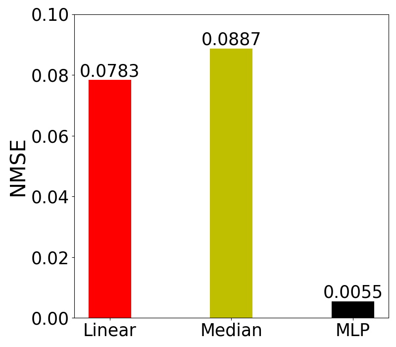
(b) NMSE comparison

Fig. 3: Patch based bad pixel correction

A n$\times$n patch may contain multiple bad pixels in the neighborhood of the central pixel, as shown in Figure 3, which makes the problem of pixel correction harder. We adopt two different approaches to mitigate this problem: increasing patch size and training models with neighborhood bad pixels. While very effective for low error rates, for high levels of image corruption they experience notable deterioration (see Section 5.2), motivating a secondary approach.

Image Reconstruction using a ViT AE: An Autoencoder (AE) [19, 20] has an encoder-decoder architecture, where the encoder learns the latent features from input images and the decoder reconstructs the image using those latent features. They are used for a wide range of vision tasks, including anomaly detection [21, 22, 20], segmentation [14, 15] and super-resolution [23, 24]. Denoising autoencoders (DAE) [19] or masked autoencoders (MAE) [18] are used as pre-training for very large models. While DAE injects noise, MAE masks out large portions of the input, and the model learns to reconstruct the image from partial input information, learning robust features.

Unlike these approaches, we use AE with the goal to recover original pixel values from corrupted images. We design a ViT based AE inspired from MAE [18]. However, differing from [18], we do not mask image portions or use mask tokens, but use the original patch embedding for the corrupted images. The AE is trained by minimizing normalized error on the corrupted pixels. We demonstrate that this method, although computationally expensive and hence inappropriate for low error rates, yields significant benefits for high rates of pixel corruption. More importantly, this method requires no prior detection, and hence, saves detection cost.

5 Experimental Results

5.1 Experimental Setup

Models and Dataset: Our approaches are evaluated on the Samsung S7 ISP [25] and the Canon EOS 5D subset of the MIT-Adobe FiveK dataset [26] datasets. The S7 ISP is a small dataset, consisting of 110 image pairs, captured using the Samsung S7 rear camera, whereas the MIT FiveK is a large-scale dataset, containing 5,000 photographs taken with SLR cameras, from which we extract 777 Canon images, similar to [27]. We consider the raw images for this task and inject bad pixels to the images to evaluate our approaches. The datasets are split into train, validation, and test sets in a ratio of 8:1:1. Detection is performed using U-Net [14] segmentation model, and correction is performed using a 2-layer MLP [28] and ViT AE, inspired from [18].

Bad pixel injection: Pixel defects in image sensors have different types. While dead pixels are permanently stuck at 0, hot pixels or stuck pixels maybe permanently bright. Pixel defects may also cause them to deviate from their original value. In our framework, the bad pixel value is obtained by adding at least $\pm\delta$ variation to original pixel value, but still within the permissible range of pixel values. We test our approach over a wide range of $\delta$. The lower the deviation from its original value, the harder it is to detect a bad pixel, whereas, higher the deviation in neighboring pixels, harder it is for correction. The number of bad pixels expected is determined by manufacturing facilities as well as sensor lifetime models. We test over a wide range of error rates from 0.01% to 85% with the location of bad pixels selected at random.

Training Framework: Both U-Net and ViT AE models are trained for 50 epochs on S7 ISP and 10 epochs on MIT FiveK datasets. For U-Net, we use a step learning rate (lr), starting with a lr of 0.001 and decaying by 0.5 every 10 epochs. ViT AE is trained with an initial lr of 0.01, a linear increase in lr for the first 5 epochs, and cosine decay in lr for the rest of the training epochs. The MLP models for correction are trained for 50 epochs using a learning rate of 0.01. Since raw images have very high dimension ($\sim$3000$\times$4000), each image is broken down into 64 patches before being fed into U-Net or ViT AE, to reduce computation.

Evaluation metrics: The detection approach is evaluated using Precision and Recall. Precision is defined as $\text{TP}/(\text{TP}+\text{FP})$ and Recall is defined as $\text{TP}/(\text{TP}+\text{FN})$ where TP, FP, and FN refer to true positives, false positives, and false negatives, respectively. In this case, bad pixels are considered positives. Thus, recall quantifies the detection rate and precision quantifies the false positive ratio. The correction approach is evaluated using NMSE given by $\frac{\lVert p_{pred}-p_{act}\rVert_{2}^{2}}{\lVert p_{act}\rVert_{2}^{2}}$ where $p_{act}$ and $p_{pred}$ refer to actual and predicted pixel values.

5.2 Results and Analysis

Table 1 summarizes the results for bad pixel detection and correction using the proposed approaches for error rates ranging from 0.01% to 70%. Detection results are reported for a single test image. While for the larger dataset MIT FiveK, we are able to achieve 99.6% detection accuracy, even with a single test image, the obtained detection rate is lower for the smaller S7 ISP dataset, due to lack of training samples. To mitigate this, we leverage prediction confidence for multiple test images (see Figure 4). NMSE values are reported for both patch-based correction using MLP (NMSE_MLP) and image reconstruction using ViT (NMSE_AE). The MLP model is trained on 5$\times$5 patches, whereas, the AE is trained on entire images, both having the specified error rate. While patch-based pixel correction is effective for low error rates, it suffers up to 31% pixel error when 70% pixels are bad. The AE model successfully reduces this error to 1.55%.

Dataset	Error	Detection		Correction
	(%)	Recall	Precision	NMSEMLP	NMSEAE
S7 ISP	0.01	0.85	0.96	0.005	0.053
	70	0.95	0.99	0.26	0.098
MIT FiveK	0.01	0.996	0.994	0.0009	0.0036
	70	0.994	0.995	0.31	0.0155

Table 1: Detection and correction results for widely different error rates (with $\delta$=0.7).

Improving Detection using Confidence Calibration: In Table 1, we observe that for the S7 ISP dataset, we are not able to detect nearly 15% of the bad pixels, even for a $\delta$ variation of 0.7. To address this, we use our confidence calibration approach. Figure 4 illustrates precision and recall values for a fixed error pattern and different $\delta$ variations, with an increase in the number of images used during inference. The increasing trend in precision as well as recall reaffirms our hypothesis, that using multiple images during test time helps in more reliable pixel detection. We observe that using 9 test images, the maximum number supported by our test set, yields an improvement of $\sim$20% in detection rate, compared with a single test image.

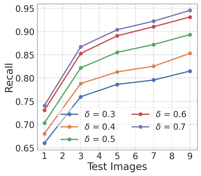
(a) Recall

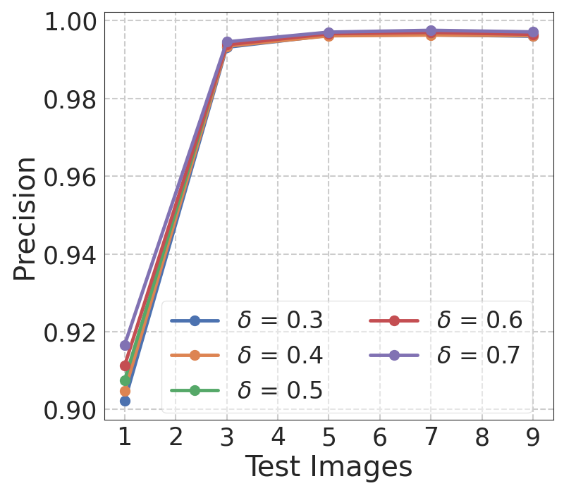
(b) Precision

Fig. 4: Precision and recall vs # of test images for confidence calibration on S7 ISP dataset (error rate=0.01%)

Necessity for Training with Corrupted Pixels: We quantify the need for models to be trained with patches containing neighborhood defects (Figure 5(a)) for patch-based correction. A model, trained using no bad pixels in the neighborhood, performs poorly when it is fed with a patch containing up to 4 bad pixels. A model, trained on multiple bad pixels, yields low error for all defect rates, although it incurs a small increase in error for no neighborhood defects. Hence, we train our models for a given error rate.

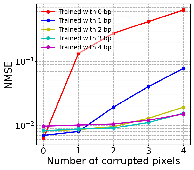
(a) Training with corrupted pixels

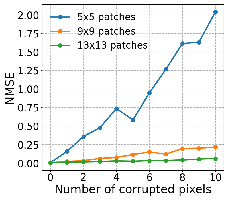
(b) Increasing patch size

Fig. 5: Patch-based pixel correction on the S7 ISP dataset

Impact of Increasing Patch Size: In Figure 5(b), we demonstrate results with increased patch size of $9\times 9$ and $13\times 13$, when there are up to 10 bad pixels in the neighborhood. The models are trained on patches with no bad pixel in the neighborhood and tested on patches with multiple bad pixels. Increasing patch size provides clear advantage when number of number of defective pixels in a patch are low.

Comparison with Interpolation Methods: For 5 erroneous pixels in a 5$\times$5 patch (error rate is 20%), our MLP model achieves a PSNR of 30.55 dB on the S7 ISP dataset, which is higher than reported for all interpolation techniques described in Section 2. More specifically, a comparison with the results reported in [2] suggests that our model exceeds ADC [8] by 7.05dB and linear [4] and median [5] interpolation by 4.85dB.

Correction using MLP vs ViT AE: In Figure 6, we compare patch based pixel correction vs AE based reconstruction for different error rates. MLP models are trained with varying patch sizes with pre-defined error rates. We observe that increasing patch size for MLP models is ineffective when the number of bad pixels scales with patch size. ViT, however, learns from the global image context and maintains a low NMSE even for very high error rates, achieving 2.2% NMSE for 85% corrupted pixels. While ViT AE performs significantly better for high error rates, patch wise detection and correction is more effective for low error rates.

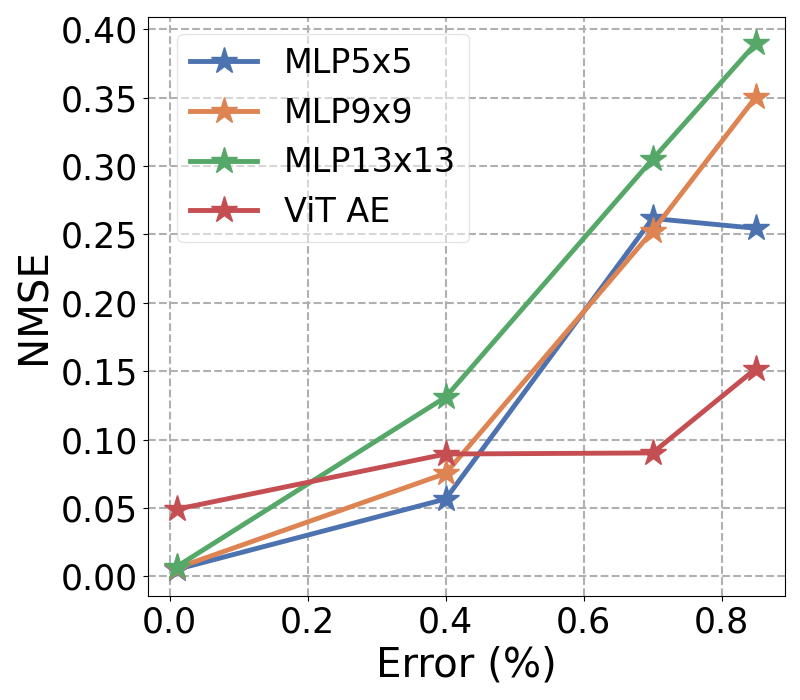
(a) Samsung S7 ISP

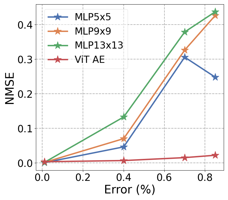
(b) MIT Adobe 5K

Fig. 6: Comparison of ViT AE and MLP based correction with S7 ISP and MIT FiveK for wide range of error rates

6 Summary and Conclusions

This paper presents novel and comprehensive DL based solutions for both the detection and correction of bad pixels for image sensors, for a wide range of error rates, and pixel variations. We achieve detection rate up to 99.6% with less than 0.6% false positives. The correction algorithm yields significantly better results than classical interpolation based approaches. We also offer a fail-safe reconstruction approach for extremely high error rates, which achieves 1.55% average pixel error for 70% corrupted pixels. Our future work includes exploring how the correction algorithm can be combined with in-sensor computing solutions.

Since our pixel detection and correction pipeline operates on the pre-ISP raw images, it can also completely bypass the ISP operations [29], which are typically expensive and performed off-chip. This also enables the pathway for our pipeline to be integrated with existing in-pixel computing paradigms [30, 31], that can significantly improve the sensor energy-efficiency for CV tasks.

Acknowledgements: We thank Dr. Souvik Kundu for his guidance in this research.

References

- [1] M. LaPedus, “Scaling CMOS image sensors,” 2020, https://semiengineering.com/scaling-cmos-image-sensors/,.
- [2] Michael Schöberl, Jürgen Seiler, Bernhard Kasper, Siegfried Fößel, and André Kaup, “Sparsity-based defect pixel compensation for arbitrary camera raw images,” 2011 IEEE International Conference on Acoustics, Speech and Signal Processing (ICASSP), pp. 1257–1260, 2011.
- [3] D.D. Pape and W.T. Reiss, “Defect correction apparatus for solid state imaging devices including inoperative pixel detection,” Sept. 10 1991, US Patent 5,047,863.
- [4] M.G. Kovac, “Removal of dark current spikes from image sensor output signals,” 1975, US Patent 3,904,818.
- [5] Su Wang, Suying Yao, Olivier Faurie, and Zaifeng Shi, “Adaptive defect correction and noise suppression module in the CIS image processing system,” in Applied Optics and Photonics China, 2009.
- [6] Girish Kalyanasundaram, Puneet Pandey, and Manjit Hota, “A pre-processing assisted neural network for dynamic bad pixel detection in Bayer images,” in International Conference on Computer Vision and Image Processing, 2020.
- [7] Eunae Lee, Eunyeong Hong, and Dong Sik Kim, “Using deep learning for pixel-defect corrections in flat-panel radiography imaging,” Journal of Medical Imaging, vol. 8, pp. 023501 – 023501, 2021.
- [8] Anthony A. Tanbakuchi, A.G. van der Sijde, Bart Dillen, Albert J. P. Theuwissen, and Wim de Haan, “Adaptive pixel defect correction,” in IS&T/SPIE Electronic Imaging, 2003.
- [9] Jenny Leung, Glenn H Chapman, Israel Koren, and Zahava Koren, “Automatic detection of in-field defect growth in image sensors,” in 2008 IEEE International Symposium on Defect and Fault Tolerance of VLSI Systems. IEEE, 2008, pp. 305–313.
- [10] Touraj Tajbakhsh, “Efficient defect pixel cluster detection and correction for bayer cfa image sequences,” in Digital Photography VII. SPIE, 2011, vol. 7876, pp. 174–182.
- [11] Noha A. El-Yamany, “Robust defect pixel detection and correction for Bayer imaging systems,” in Digital Photography and Mobile Imaging, 2017.
- [12] Jie Chen, Binghao Wang, Shupei He, Qijun Xing, Xing Su, Wei Liu, and Ge Gao, “Hisp: Heterogeneous image signal processor pipeline combining traditional and deep learning algorithms implemented on fpga,” Electronics, vol. 12, no. 16, pp. 3525, 2023.
- [13] Jonathan Long, Evan Shelhamer, and Trevor Darrell, “Fully convolutional networks for semantic segmentation,” in Proceedings of the IEEE conference on computer vision and pattern recognition, 2015, pp. 3431–3440.
- [14] Olaf Ronneberger, Philipp Fischer, and Thomas Brox, “U-net: Convolutional networks for biomedical image segmentation,” in Medical Image Computing and Computer-Assisted Intervention – MICCAI 2015, Nassir Navab, Joachim Hornegger, William M. Wells, and Alejandro F. Frangi, Eds., Cham, 2015, pp. 234–241, Springer International Publishing.
- [15] Liang-Chieh Chen, George Papandreou, Iasonas Kokkinos, Kevin Murphy, and Alan L Yuille, “DeepLab: Semantic image segmentation with deep convolutional nets, atrous convolution, and fully connected crfs,” IEEE transactions on pattern analysis and machine intelligence, vol. 40, no. 4, pp. 834–848, 2017.
- [16] Michal Drozdzal, Eugene Vorontsov, Gabriel Chartrand, Samuel Kadoury, and Chris Pal, “The importance of skip connections in biomedical image segmentation,” in International Workshop on Deep Learning in Medical Image Analysis, International Workshop on Large-Scale Annotation of Biomedical Data and Expert Label Synthesis. Springer, 2016, pp. 179–187.
- [17] Alexey Dosovitskiy, Lucas Beyer, Alexander Kolesnikov, Dirk Weissenborn, Xiaohua Zhai, Thomas Unterthiner, Mostafa Dehghani, Matthias Minderer, Georg Heigold, Sylvain Gelly, Jakob Uszkoreit, and Neil Houlsby, “An image is worth 16x16 words: Transformers for image recognition at scale,” in International Conference on Learning Representations, 2021.
- [18] Kaiming He, Xinlei Chen, Saining Xie, Yanghao Li, Piotr Dollár, and Ross Girshick, “Masked autoencoders are scalable vision learners,” in Proceedings of the IEEE/CVF conference on computer vision and pattern recognition, 2022, pp. 16000–16009.
- [19] Pascal Vincent, Hugo Larochelle, Yoshua Bengio, and Pierre-Antoine Manzagol, “Extracting and composing robust features with denoising autoencoders,” in Proceedings of the 25th international conference on Machine learning, 2008, pp. 1096–1103.
- [20] Jinwon An and Sungzoon Cho, “Variational autoencoder based anomaly detection using reconstruction probability,” Special lecture on IE, vol. 2, no. 1, pp. 1–18, 2015.
- [21] Chong Zhou and Randy C Paffenroth, “Anomaly detection with robust deep autoencoders,” in Proceedings of the 23rd ACM SIGKDD international conference on knowledge discovery and data mining, 2017, pp. 665–674.
- [22] Yiru Zhao, Bing Deng, Chen Shen, Yao Liu, Hongtao Lu, and Xian-Sheng Hua, “Spatio-temporal autoencoder for video anomaly detection,” in Proceedings of the 25th ACM international conference on Multimedia, 2017, pp. 1933–1941.
- [23] Chao Dong, Chen Change Loy, Kaiming He, and Xiaoou Tang, “Image super-resolution using deep convolutional networks,” IEEE transactions on pattern analysis and machine intelligence, vol. 38, no. 2, pp. 295–307, 2015.
- [24] Xiaojiao Mao, Chunhua Shen, and Yu-Bin Yang, “Image restoration using very deep convolutional encoder-decoder networks with symmetric skip connections,” Advances in neural information processing systems, vol. 29, 2016.
- [25] Eli Schwartz, Raja Giryes, and Alexander M. Bronstein, “DeepISP: Toward learning an end-to-end image processing pipeline,” IEEE Transactions on Image Processing, vol. 28, pp. 912–923, 2018.
- [26] Vladimir Bychkovsky, Sylvain Paris, Eric Chan, and Frédo Durand, “Learning photographic global tonal adjustment with a database of input / output image pairs,” in The Twenty-Fourth IEEE Conference on Computer Vision and Pattern Recognition, 2011.
- [27] Yazhou Xing, Zian Qian, and Qifeng Chen, “Invertible image signal processing,” in CVPR, 2021.
- [28] Yann LeCun, Yoshua Bengio, and Geoffrey Hinton, “Deep learning,” nature, vol. 521, no. 7553, pp. 436–444, 2015.
- [29] Gourav Datta, Zeyu Liu, Zihan Yin, Linyu Sun, Akhilesh R. Jaiswal, and Peter A. Beerel, “Enabling ISPless low-power computer vision,” 2023 IEEE/CVF Winter Conference on Applications of Computer Vision (WACV), pp. 2429–2438, 2022.
- [30] Gourav Datta, Souvik Kundu, Zihan Yin, Ravi Teja Lakkireddy, Peter A. Beerel, Ajey P. Jacob, and Akhilesh R. Jaiswal, “A processing-in-pixel-in-memory paradigm for resource-constrained tinyml applications,” Scientific Reports, vol. 12, 2022.
- [31] Gourav Datta, Zeyu Liu, Md Abdullah-Al Kaiser, Souvik Kundu, Joe Mathai, Zihan Yin, Ajey P. Jacob, Akhilesh R. Jaiswal, and Peter A. Beerel, “In-sensor & neuromorphic computing are all you need for energy efficient computer vision,” in ICASSP 2023 - 2023 IEEE International Conference on Acoustics, Speech and Signal Processing (ICASSP), 2023, pp. 1–5.