Multivariate sensitivity adaptive polynomial chaos expansion for vector valued surrogate modeling

Abstract

This work develops a novel basis adaptive method for constructing anisotropic polynomial chaos expansions of multidimensional (vector valued) model responses. The suggested method selects the most influential expansion terms adaptively, based on multivariate sensitivity analysis metrics that can be estimated by post-processing the polynomial chaos expansion. It is able to construct anisotropic polynomial chaos expansions and mitigate complexities due to high dimensional model inputs, while simultaneously allowing approximations of model responses with sizes up to the order of thousands. The vector valued polynomial chaos surrogate model is computed at a much smaller computational cost compared to existing sparse and/or basis adaptive polynomial chaos expansion methods, which must be applied element-wise over the multidimensional response and produce one polynomial basis per response element. Contrarily, a common basis is obtained with the suggested method, leading to major savings in terms of computational demand, while also achieving comparable approximation accuracy. Numerical investigations on different engineering test cases illustrate the advantages of the multivariate sensitivity adaptive polynomial chaos expansion method over competing approaches.

[aff1] organization=Siemens AG, Technology,city=Munich, country=Germany

[aff2] organization=Technische Universität Darmstadt, Institute for Accelerator Science and Electromagnetic Fields (TEMF),city=Darmstadt, country=Germany

1 Introduction

The polynomial chaos expansion (PCE) method is commonly employed in various forms [1] for surrogate modeling and uncertainty quantification (UQ) in scientific and engineering applications. Therein, the PCE offers inexpensive polynomial approximations of complex numerical models, commonly referred to as surrogate models, to be used in computationally demanding design tasks such as optimization and reliability analysis [2, 3, 4], or for online model based estimations in real time, e.g., in the context of digital twin applications [5]. Additionally, uncertainty and sensitivity metrics regarding the model response can be estimated by simply post-processing the expansion’s terms [6, 7, 8]. Particularly popular are the regression based variants of the PCE, where the expansion’s coefficients are computed by means of least squares regression [9, 10, 11]. In that case, the PCE is essentially a supervised machine learning model, with the additional benefit of typically requiring few training data and little computation time compared to other data-driven modeling methods [12].

One of the bottlenecks of the PCE method is the so-called “curse of dimensionality”, which in this case concerns the rapid growth of the polynomial basis, caused by large input dimensionality and high polynomial degrees. For regression based PCE methods, this can lead to an ill-conditioned, ill-posed, or simply intractable least squares problem, since the training data demand rises according to the size of the polynomial basis. This issue is particularly relevant for numerous engineering applications, where data are typically hard to obtain or expensive to generate. Remedies have been sought in sparse and/or basis adaptive PCE methods. These methods exploit anisotropies in the impact of the input parameters upon the model response, and use them to construct anisotropic polynomial bases of reduced size, which also improve the performance of the PCE in terms of accuracy versus data demand. Extensive reviews on sparse and/or basis adaptive, regression based PCE methods can be found in the works of Lüthen et al. [13, 14].

On the one hand, sparse PCEs are computed by solving a regularized least squares problem that induces sparsity in its solution and then omitting the zero coefficients. Common methods for computing sparse PCEs are least angle regression (LAR) [15], orthogonal matching pursuit (OMP) [16], and compressive sensing [17, 18, 19, 20]. On the other hand, basis adaptive PCEs are computed by progressively enriching the polynomial basis with terms of high impact, while low-impact terms are neglected. Various approaches and criteria have been suggested in the literature for adaptive basis selection, for example, based on cross-validation errors [15, 16, 21], coefficient confidence intervals [22], entropy principles [23], or variance contribution [24, 25]. Considering non-trivial applications of practical value, sparse and/or basis adaptive PCEs are generally applicable for up to moderately high dimensional inputs, typically in the order of tens or, less commonly, hundreds. In the case of very high dimensional inputs, linear dimension reduction methods such as the Karhunen-Loève expansion are most commonly employed to enable the use of PCEs [26]. More recently, nonlinear dimension reduction methods have also been used for that purpose [27, 28].

The dimensionality of the model’s response is also a cause for concern regarding the computational cost of regression based PCE methods, as the least squares problem must be solved $M$ times, where $M$ denotes the dimension of the response. Particularly considering high dimensional responses, e.g., time-series or frequency responses [29, 30], the computational cost for computing the PCE may become unfeasible. This is particularly troublesome if sparse and/or basis adaptive PCE methods are used, since most, if not all, of the available methods have been developed considering scalar model responses and rely on iterative algorithms that cannot be efficiently vectorized. For a multidimensional model response, they must be applied element-wise, often resulting in too high computation times. To render sparse and/or basis adaptive PCE methods tractable, dimension reduction techniques are used to reduce the dimensionality of the response to its minimum necessary components. Most commonly, linear dimension reduction is used, e.g., based on principal component analysis (PCA) or proper orthogonal decomposition (POD) [31, 32, 33, 34, 35]. Nonlinear dimension reduction has also been considered recently [36]. However, even after the application of dimension reduction techniques, the effective dimension of the response may remain comparatively high, thus still resulting in an unacceptable computational cost.

This paper suggests a new basis adaptive PCE method that specifically targets multidimensional model responses. Its main novelty lies in the adaptive basis selection approach, which utilizes the metrics of a multivariate global sensitivity analysis (GSA) method [37]. The latter can be seen as a generalization of the well-known Sobol sensitivity analysis [38] from scalar to functional and vector valued model responses. Similar to the Sobol indices, the multivariate sensitivity indices can be estimated by post-processing the vector valued PCE [39, 40] and correspond to contributions to the aggregated variance over the multidimensional model response. Accordingly, the vector valued PCE coefficients can be interpreted as multivariate sensitivity indicators. Basis enrichment is then performed according to the multivariate sensitivity indicators, such that the terms included in the expansion are the ones with the maximum contribution to the aggregated variance of the vector valued model response. With respect to the candidate terms for basis enrichment, a forward neighbor approach is used [14], such that the polynomial basis remains downward closed [41]. We call the suggested basis adaptive PCE method multivariate sensitivity adaptive (MVSA).

The MVSA PCE method developed in this work differs substantially from PCE methods available in the literature, which also address the case of multidimensional model responses [31, 32, 33, 34, 29, 35, 30]. Using the multivariate GSA based basis selection criterion, the MVSA algorithm constructs a single anisotropic polynomial basis for the model response. This is an important distinction to approaches that iterate over the elements of the response and construct one basis per element. The common polynomial basis allows the use of vectorized ordinary least squares (OLS) solvers, leading to significantly reduced computation times. To ensure that the OLS problem remains well-conditioned, the system matrix is monitored during the basis enrichment process, such that its condition number does not exceed a predefined threshold [25]. The common basis and the vectorized OLS solver also allow the MVSA PCE method to be applied to model responses with sizes up to the order of thousands, which is too computationally expensive otherwise. Hence, the applicability of the method does not depend on a reduced effective dimension, equivalently, it is not necessary to be combined with dimension reduction techniques. On possible downsides, the common basis obtained with the MVSA algorithm is expected to be sub-optimal considering all elements of the model response, possibly leading to reduced approximation accuracy compared to the alternative of a unique basis per response element. Nonetheless, our numerical investigations indicate that the MVSA PCE remains on par with competing approaches in terms of accuracy, even outperforming them in certain cases, while at the same time being massively more efficient in terms of computation time.

The remaining of this paper is structured as follows. Section 2 describes the general problem setting of parameter dependent models with random inputs. Section 3 recalls variance based GSA methods for scalar and multidimensional (vector valued) model responses. Section 4 discusses the PCE method, its computation by means of regression, and its connection to GSA. Section 5 presents the MVSA PCE method for the construction of anisotropic vector valued PCEs. In Section 6, the MVSA PCE method is applied for surrogate modeling in different engineering test cases and compared against competing basis adaptive and sparse PCE methods. Our conclusions are discussed in Section 7.

2 Parameter dependent model with random input data

In the following, we shall consider a parameter dependent model $f(\mathbf{x})$, such that

$$f\colon\mathbf{x}\to\mathbf{y},\>\text{equivalently},\>\mathbf{y}=f\left(\mathbf{x}\right),$$ (1)

where $\mathbf{x}\in\mathbb{R}^{N}$ is an input parameter vector and $\mathbf{y}\in\mathbb{R}^{M}$ the corresponding model response. The model, which is here abstractly given as the function $f$, is considered to be deterministic, meaning that its response cannot vary given the same input. Throughout this work, the model’s input parameters $\mathbf{x}$ are considered to be realizations of a random vector $\mathbf{X}=(X_{1},X_{2},\dots,X_{N})^{\top}$, where $X_{n},\,n=1,2,\dots,N$, are assumed to be independent random variables. The multivariate random variable $\mathbf{X}$ is defined on the probability space $(\Theta,\Sigma,P)$, where $\Theta$ is the sample space, $\Sigma$ the sigma algebra of events, and $P\colon\Sigma\to[0,1]$ a probability measure. Accordingly, $\mathbf{x}=\mathbf{X}(\theta)\in\Xi$ is a random variable realization for $\theta\in\Theta$, where $\Xi\subset\mathbb{R}^{N}$ is called the image space. The random vector is additionally characterized by the probability density function (PDF) $\varrho_{\mathbf{X}}(\mathbf{x})\colon\Xi\to\mathbb{R}_{\geq 0}$. Under the independence assumption for the random variables $X_{n}$, it holds that $\varrho_{\mathbf{X}}(\mathbf{x})=\prod_{n=1}^{N}\varrho_{X_{n}}(x_{n})$ and $\Xi=\Xi_{1}\times\cdots\times\Xi_{N}$, where $\varrho_{X_{n}}(x_{n})$ and $\Xi_{n}$ are the marginal (univariate) PDFs and image spaces, respectively. Due to the propagation of uncertainty through the model, its response is now a dependent random variable $\mathbf{Y}=f(\mathbf{X})$.

3 Global sensitivity analysis

Global sensitivity analysis (GSA) is broadly defined as the study of how uncertainty in the response of a model can be allocated to the considered input uncertainty sources [42]. We are interested in variance based GSA, also referred to as the Sobol method [38, 43]. The corresponding sensitivity metrics are known as Sobol indices. Note that the Sobol method concerns scalar model responses only. Extensions were developed later to address multidimensional model responses [44, 37].

3.1 Global sensitivity analysis for scalar model response

We consider a parametric model similar to the one described in Section 2, however, with a scalar response $y=f(\mathbf{x})\in\mathbb{R}$. The Sobol method begins with a decomposition of the scalar random response $Y=f(\mathbf{X})$, such that

$$Y=f\left(\mathbf{X}\right)=f_{0}+\sum_{n=1}^{N}f_{n}\left(X_{n}\right)+\sum_{n<k}^{N}f_{nk}\left(X_{n},X_{k}\right)+\cdots+f_{1,\dots,N}\left(X_{1},\dots,X_{N}\right),$$ (2)

where $f_{0}$ is a constant function, $f_{n}$ is a function of $X_{n}$ only, $f_{nk}$ is a function of $X_{n}$ and $X_{k}$, and so forth. The terms of (2) are proven to be orthogonal [43], therefore, the expected value of the response is $\mathbb{E}\left[Y\right]=f_{0}$. Then, the variance $\mathbb{V}\left[Y\right]$ can be decomposed as

$$\mathbb{V}\left[Y\right]=\sum_{n=1}^{N}\mathbb{V}\left[f_{n}\right]+\sum_{n<k}^{N}\mathbb{V}\left[f_{nk}\right]+\cdots+\mathbb{V}\left[f_{1,\dots,N}\right]=\sum_{n=1}^{N}\mathbb{V}_{n}+\sum_{n<k}^{N}\mathbb{V}_{nk}+\cdots+\mathbb{V}_{1,\dots,N},$$ (3)

where $\mathbb{V}_{n}$ is a partial variance attributed only to $X_{n}$, $\mathbb{V}_{nk}$ is a partial variance attributed to the combination of $X_{n}$ and $X_{k}$, and so forth. First-order Sobol indices quantify the impact of the random variable $X_{n}$ alone, i.e., with all other parameters regarded as constant, and are given as

$$S_{n}^{\text{F}}=\frac{\mathbb{V}_{n}}{\mathbb{V}\left[Y\right]}.$$ (4)

Total-effect Sobol indices quantify the impact of the random variable $X_{n}$ when interacting with all remaining random variables $X_{k}$, $k\neq n$, and are given as

$$S_{n}^{\text{T}}=\frac{1}{\mathbb{V}\left[Y\right]}\left(\mathbb{V}_{n}+\sum_{\begin{subarray}{c}n<k\end{subarray}}^{N}\mathbb{V}_{nk}+\cdots+\mathbb{V}_{1,\dots,N}\right).$$ (5)

Sobol indices quantifying other interactions among the random variables, e.g., second- or third-order, can be computed in a similar manner [42].

3.2 Global sensitivity analysis for vector valued model response

We now consider a multidimensional random response $\mathbf{Y}=\left(Y_{1},\dots,Y_{M}\right)$ and the dependence $\mathbf{Y}=f(\mathbf{X})$, as described in Section 2. In principle, the GSA method presented in Section 3.1 can be applied element-wise to each scalar component $Y_{m}$, $m=1,\dots,M$. However, correlations among the response’s components render this approach questionable, as it may lead to redundant and difficult to interpret results [45, 46]. To circumvent this impasse, two multivariate GSA methodologies have been developed, based on decomposing either the vector valued response itself [44] or the corresponding covariance matrix [37]. Both approaches compute generalised sensitivity indices that quantify the impact of the input random variables on the full multivariate response. In fact, the generalised sensitivity indices provided by these two multivariate GSA approaches are equivalent [39].

Following the work of Gamboa et al. [37], we consider a non-empty index set $\mathbf{u}\subset(1,\dots,N)$, its complement $\mathbf{v}=(1,\dots,N)\setminus\mathbf{u}$, and the corresponding input random variable subsets $\mathbf{X}_{\mathbf{u}}=\left\{X_{n}\right\}_{n\in\mathbf{u}}$, $\mathbf{X}_{\mathbf{v}}=\left\{X_{n}\right\}_{n\in\mathbf{v}}$. By applying the Hoeffding decomposition [47], we obtain the output decomposition

$$\mathbf{Y}=f(\mathbf{X})=f_{0}+f_{\mathbf{u}}(\mathbf{X}_{\mathbf{u}})+f_{\mathbf{v}}(\mathbf{X}_{\mathbf{v}})+f_{\mathbf{u},\mathbf{v}}(\mathbf{X}_{\mathbf{u}},\mathbf{X}_{\mathbf{v}}),$$ (6)

where $f_{0}\in\mathbb{R}^{M}$, $f_{\mathbf{u}}:\mathbb{R}^{\#\mathbf{u}}\rightarrow\mathbb{R}^{M}$, $f_{\mathbf{v}}:\mathbb{R}^{\#\mathbf{v}}\rightarrow\mathbb{R}^{M}$, and $f_{\mathbf{u},\mathbf{v}}:\mathbb{R}^{N}\rightarrow\mathbb{R}^{M}$, where $\#$ denotes the cardinality of a set. Taking the covariance matrices in both sides of (6) yields

$$\mathbf{C}=\mathbf{C}_{\mathbf{u}}+\mathbf{C}_{\mathbf{v}}+\mathbf{C}_{\mathbf{u},\mathbf{v}},$$ (7)

where $\mathbf{C}$, $\mathbf{C}_{\mathbf{u}}$, $\mathbf{C}_{\mathbf{v}}$, and $\mathbf{C}_{\mathbf{u},\mathbf{v}}$ are the covariance matrices for $f$ (equivalently, for $\mathbf{Y}$), $f_{\mathbf{u}}$, $f_{\mathbf{v}}$, and $f_{\mathbf{u},\mathbf{v}}$, respectively. By considering index sets comprising single indices, index pairs, triplets, and so forth, the covariance decomposition (7) can be written as

$$\mathbf{C}=\sum_{n=1}^{N}\mathbf{C}_{n}+\sum_{n<k}\mathbf{C}_{nk}+\cdots+\mathbf{C}_{1,\dots,N},$$ (8)

which is the multidimensional analog to the variance decomposition (3). In fact, for a scalar response, decomposition (3) is recovered from (8). Based on this observation, generalised sensitivity indices for multidimensional responses are motivated as follows. The sum of the variances of all response components $Y_{m}$, $m=1,\dots,M$, is equal to $\mathrm{tr}(\mathbf{C})$ and corresponds to the aggregated variance of the multidimensional response. Then, the multivariate equivalent to the first-order Sobol index (4) is obtained as

$$G_{n}^{\text{F}}=\frac{\mathrm{tr}\left(\mathbf{C}_{n}\right)}{\mathrm{tr}\left(\mathbf{C}\right)},$$ (9)

where the numerator quantifies the aggregated variance caused by the random variable $X_{n}$ alone. In analogous fashion, the multivariate counterpart to the total-effect Sobol index (5) is given by

$$G_{n}^{\text{T}}=\frac{\mathrm{tr}\left(\mathbf{C}_{n}\right)+\sum_{n<k}\mathrm{tr}\left(\mathbf{C}_{nk}\right)+\cdots+\mathrm{tr}\left(\mathbf{C}_{1,\dots,N}\right)}{\mathrm{tr}\left(\mathbf{C}\right)}.$$ (10)

4 Polynomial chaos expansion

The polynomial chaos expansion (PCE) originates from the work of Wiener [48], but was popularized much later as an efficient uncertainty quantification (UQ) method [26, 49]. Recall from Section 2 the (dependent) random model response $\mathbf{Y}=f(\mathbf{X})$, with $\mathbf{Y}=\left(Y_{1},\dots,Y_{M}\right)$ and $\mathbf{X}=\left(X_{1},\dots,X_{N}\right)$, and the fixed response $\mathbf{y}=f(\mathbf{x})$ for $\mathbf{x}=\mathbf{X}\left(\theta\right)$. Then, a PCE is a global polynomial approximation of the form

$$f(\mathbf{x})\approx\widetilde{f}(\mathbf{x})=\sum_{k=1}^{K}\mathbf{c}_{k}\Psi_{k}(\mathbf{x}),$$ (11)

where $\mathbf{c}_{k}\in\mathbb{R}^{M}$ are the expansion coefficients and $\Psi_{k}$ are multivariate polynomials that satisfy the orthogonality property

$$\mathbb{E}\left[\Psi_{k}\Psi_{l}\right]=\int_{\Xi}\Psi_{k}\left(\mathbf{x}\right)\Psi_{l}\left(\mathbf{x}\right)\varrho_{\mathbf{X}}\left(\mathbf{x}\right)\mathrm{d}\mathbf{x}=\mathbb{E}\left[\Psi_{k}^{2}\right]\delta_{kl},$$ (12)

where $\delta_{kl}$ is the Kronecker delta. Depending on the distribution of the random inputs, the polynomials are either selected according to the Wiener-Askey scheme [49] or constructed numerically [50, 51, 52]. In the remaining of this paper, we always consider orthonormal polynomials, such that $\mathbb{E}\left[\Psi_{k}^{2}\right]=1$. As mentioned in Section 2, the input random variables are assumed to be independent, hence, the joint probability density function (PDF) is given as $\varrho_{\mathbf{X}}\left(\mathbf{x}\right)=\prod_{n=1}^{N}\varrho_{X_{n}}\left(x_{n}\right)$. Note that it is possible to construct PCEs for dependent input random variables also [53, 54, 55]. The multivariate orthogonal polynomials are constructed as

$$\Psi_{k}(\mathbf{x})=\Psi_{\mathbf{k}}(\mathbf{x})=\prod_{n=1}^{N}\psi_{n}^{k_{n}}(x_{n}),$$ (13)

where $\psi_{n}^{k_{n}}$ are univariate polynomials of degree $k_{n}$ and orthogonal, respectively, orthonormal with respect to the corresponding marginal PDFs $\varrho_{X_{n}}$, and $\mathbf{k}=\left(k_{1},\dots,k_{N}\right)$. The PCE (11) can now be equivalently written as

$$f(\mathbf{x})\approx\widetilde{f}(\mathbf{x})=\sum_{\mathbf{k}\in\Lambda}\mathbf{c}_{\mathbf{k}}\Psi_{\mathbf{k}}(\mathbf{x}),$$ (14)

where the multi-indices $\mathbf{k}=\left(k_{1},\dots,k_{N}\right)$ in (14) are uniquely associated to the single indices $k$ in (11) and $\Lambda$ is a multi-index set with cardinality $\#\Lambda=K$.

It is typical to use a multi-index set $\Lambda$ corresponding to a total degree basis, where $\Lambda=\left\{\mathbf{k}:\lVert\mathbf{k}\rVert_{1}\leq p\right\}$ for maximum univariate polynomial degree $p\in\mathbb{Z}_{\geq 0}$. Another common option is the hyperbolic truncation basis, where $\Lambda=\left\{\mathbf{k}:\lVert\mathbf{k}\rVert_{q}\leq p\right\}$, with $q\in\left(0,1\right)$ and $\lVert\mathbf{k}\rVert_{q}=\left(\sum_{n=1}^{N}\left(k_{n}\right)^{q}\right)^{1/q}$. Note that both bases are isotropic, meaning that the same univariate basis terms are considered for all inputs $X_{n}$, $n=1,\dots,N$. As a result, the basis grows rapidly for an increasing maximum polynomial degree $p$ and, more crucially, for a high dimensional input parameter vector $\mathbf{X}$, which is a manifestation of the so called curse of dimensionality.

4.1 Regression based computation of polynomial chaos expansion coefficients

In this work, the coefficients of the PCE are computed by means of regression [15, 10]. Alternative options include pseudo-spectral projection [56, 57, 58] and, less commonly, interpolation [59, 60]. Collecting the PCE coefficients $\mathbf{c}_{k}\in\mathbb{R}^{M}$, $k=1,\dots,K$, into a matrix $\boldsymbol{\Gamma}\in\mathbb{R}^{K\times M}$, such that the coefficient $\mathbf{c}_{k}$ is the $k$-th row of $\boldsymbol{\Gamma}$, the coefficients are computed by solving the least squares regression problem

$$\underset{\boldsymbol{\Gamma}\in\mathbb{R}^{K\times M}}{\arg\min}\left\{\frac{1}{Q}\sum_{q=1}^{Q}\left(\mathbf{y}^{(q)}-\sum_{k=1}^{K}\mathbf{c}_{k}\Psi_{k}\left(\mathbf{x}^{(q)}\right)\right)^{2}\right\},$$ (15)

where $\left\{\mathbf{x}^{(q)},\mathbf{y}^{(q)}=f\left(\mathbf{x}^{(q)}\right)\right\}_{q=1}^{Q}$ is a set of input parameter realizations along with the corresponding model responses, called the experimental design or the training data set. In matrix format, the regression problem (15) is equivalently written as

$$\underset{\boldsymbol{\Gamma}\in\mathbb{R}^{K\times M}}{\arg\min}\left\{\frac{1}{Q}\lVert\mathbf{B}-\mathbf{D}\boldsymbol{\Gamma}\rVert_{2}\right\},$$ (16)

where $\mathbf{D}\in\mathbb{R}^{Q\times K}$ with $d_{qk}=\Psi_{k}\left(\mathbf{x}^{(q)}\right)$ is the least squares system matrix, also called the design matrix, and $\mathbf{B}\in\mathbb{R}^{Q\times M}$ with $b_{qm}=y_{m}^{(q)}$ the right hand side.

For the regression problem to be well posed and uniquely solvable with an ordinary least squares (OLS) solver, the size of the experimental design must be at least equal to the size of the polynomial basis, i.e., $Q\geq K$. For a well conditioned OLS problem, $Q$ is typically chosen to be 2–5 times larger than $K$, depending on the problem at hand [41, 11]. This can lead to severe computational problems if the polynomial basis is too large, e.g., for a total degree basis with high maximum polynomial degree $p$ and input dimensionality. This limitation can be overcome by methods that penalize (15)–(16) to compute sparse solutions [13], for example using the least absolute shrinkage and selection operator (LASSO) method [61] or compressive sensing [62]. Sparse solutions are typically computed using iterative algorithms such as least angle regression (LAR) [15], orthogonal matching pursuit (OMP) [16], or subspace pursuit (SP) [18]. Alternatively, basis adaptive algorithms can be used [14], where the basis is sequentially enriched with new terms, up to a size that does not lead to conditioning issues. A limitation here is that the sparse and/or basis adaptive PCE algorithms available in the literature consider scalar model responses almost exclusively, therefore, must be applied element-wise for each of the $M$ components of a vector valued model response. This can lead to an undesirable computational cost with respect to the computation of the PCE coefficients, especially if the response is high dimensional.

4.2 Global sensitivity analysis based on polynomial chaos expansion

For a PCE approximation in the form of (14), it is straightforward to show that the mean and variance of the response can be estimated as

$$\mathbb{E}\left[Y\right] \approx\mathbf{c}_{\mathbf{0}},$$ (17a)

$$\mathbb{V}\left[Y\right] \approx\sum_{\mathbf{k}\in\Lambda\setminus\mathbf{0}}\mathbf{c}_{\mathbf{k}}^{2},$$ (17b)

where the zeroth multi-index is denoted as $\mathbf{0}=\left(0,\dots,0\right)$ and the PCE basis is considered to be orthonormal [26].

For a scalar response $Y=f\left(\mathbf{X}\right)$, the PCE takes the form of the Sobol decomposition (2) by appropriately ordering its terms. Hence, Sobol sensitivity indices can be estimated by simply post-processing the PCE [6, 8]. Indeed, the PCE coefficients $c_{\mathbf{k}}$ for $\mathbf{k}\in\Lambda\setminus\mathbf{0}$ can be interpreted as partial variances due to specific random variable interactions defined by the multi-indices $\mathbf{k}$. The multi-indices corresponding to partial variances caused by $X_{n}$, either individually (first-order) or in combination with all other random variables (total-effect), can then be collected into the multi-index sets $\Lambda_{n}^{\text{F}}\subset\Lambda$ and $\Lambda_{n}^{\text{T}}\subset\Lambda$, respectively defined as

$$\Lambda_{n}^{\text{F}} =\{\mathbf{k}\in\Lambda\;:\;k_{n}\neq 0\>\>\text{and}\>\>k_{l}=0,l=1,\dots,N,l\neq n\},$$ (18a)

$$\Lambda_{n}^{\text{T}} =\{\mathbf{k}\in\Lambda\;:\;k_{n}\neq 0\}.$$ (18b)

The first-order and total-effect Sobol indices are then estimated as

$$S_{n}^{\text{F}} \approx\frac{\sum_{\mathbf{k}\in\Lambda_{n}^{\text{F}}}c_{\mathbf{k}}^{2}}{\sum_{\mathbf{k}\in\Lambda\setminus\mathbf{0}}c_{\mathbf{k}}^{2}},$$ (19a)

$$S_{n}^{\text{T}} \approx\frac{\sum_{\mathbf{k}\in\Lambda_{n}^{\text{T}}}c_{\mathbf{k}}^{2}}{\sum_{\mathbf{k}\in\Lambda\setminus\mathbf{0}}c_{\mathbf{k}}^{2}}.$$ (19b)

For a multidimensional response $\mathbf{Y}=f\left(\mathbf{X}\right)$, multivariate global sensitivity analysis (GSA) requires the computation of the traces of the covariance matrices with respect to the components $Y_{m}$, which depend on specific combinations of the input random variables, as shown in Section 3.2. The traces are equal to the sum of the variances of all response components dependent on the specific input random variable combinations. Similar to the case of a scalar response, the partial variances are easily computed from the PCE coefficients [39]. Then, the generalised sensitivity indices $G_{n}^{\text{F}}$ and $G_{n}^{\text{T}}$ defined in (9) and (10), respectively, can be estimated as

$$G_{n}^{\text{F}} \approx\frac{\sum_{m=1}^{M}\left(\sum_{\mathbf{k}\in\Lambda_{n}^{\text{F}}}c_{m,\mathbf{k}}^{2}\right)}{\sum_{m=1}^{M}\left(\sum_{\mathbf{k}\in\Lambda\setminus\mathbf{0}}c_{m,\mathbf{k}}^{2}\right)},$$ (20a)

$$G_{n}^{\text{T}} \approx\frac{\sum_{m=1}^{M}\left(\sum_{\mathbf{k}\in\Lambda_{n}^{\text{T}}}c_{m,\mathbf{k}}^{2}\right)}{\sum_{m=1}^{M}\left(\sum_{\mathbf{k}\in\Lambda\setminus\mathbf{0}}c_{m,\mathbf{k}}^{2}\right)}.$$ (20b)

Accordingly, a vector valued PCE coefficient $\mathbf{c}_{\mathbf{k}}=\left(c_{m,\mathbf{k}}\right)_{1\leq m\leq M}$ yields a contribution to the aggregated variance over the multidimensional model response, that is specific to the multi-index $\mathbf{k}$.

Note that the use of a common multi-index set $\Lambda$ in (20) implies that the PCE basis is the same for all response elements. This is not necessarily true, for example, if a sparse and/or adaptive PCE methods is applied element-wise over the response, or for isotropic PCEs with different maximum polynomial degrees per response element. In that case, multi-index sets $\Lambda_{m}$, $\Lambda_{m,n}^{\text{F}}$, and $\Lambda_{m,n}^{\text{T}}$, $m=1,\dots,M$, must be used for the PCE based estimation of the generalized sensitivity indices.

5 Multivariate sensitivity adaptive polynomial chaos expansion

In the multivariate sensitivity adaptive (MVSA) polynomial chaos expansion (PCE) method, the polynomial basis is expanded sequentially, such that the newly added expansion terms are the ones corresponding to the maximum contribution to the aggregated variance of the multidimensional model response (see Sections 3.2 and 4.2). In that way, a common multi-index set $\Lambda$ and polynomial basis are constructed for the vector valued response. The candidate terms are selected based on a forward neighbor approach [16, 14], such that the multi-index set remains downward closed [41]. The PCE coefficients are computed with an ordinary least squares (OLS) solver. The sequential basis expansion is terminated if the OLS problem becomes ill-posed or ill-conditioned. The main steps and building blocks of the MVSA PCE method are explained in detail in the following. The complete procedure is also described in Algorithm 1.

1

Data: Training data set $\left\{\mathbf{x}^{(q)},\mathbf{y}^{(q)}=f\left(\mathbf{x}^{(q)}\right)\right\}_{q=1}^{Q}$ with $\mathbf{x}^{(q)}\in\mathbb{R}^{N}$ and $\mathbf{y}^{(q)}\in\mathbb{R}^{M}$, initial downward closed multi-index set $\Lambda_{\text{init}}$ with $\#\Lambda_{\text{init}}<Q$, maximum condition number $\kappa$.

Result: Multi-index set $\Lambda$ and corresponding PCE.

2

3Set $\Lambda=\Lambda_{\text{init}}$.

4while True do // adaptive basis expansion

5      

6      Compute the admissible multi-index set $\Lambda^{+}_{\text{adm}}$ as in (23).

7      Construct the extended multi-index set $\Lambda_{\text{ext}}=\Lambda\cup\Lambda^{+}_{\text{adm}}$.

8      if $\#\Lambda_{\mathrm{ext}}>Q$ then // underdetermined OLS problem

9             Exit while-loop.

10       end if

11      

12      Solve the OLS problem (15), equivalently (16), for the extended multi-index set $\Lambda_{\text{ext}}$.

13      if $\mathrm{cond}\left(\mathbf{D}_{\mathrm{ext}}\right)>\kappa$ then // ill-conditioned OLS problem

14             Exit while-loop.

15       end if

16      

17      Find the multi-index $\mathbf{k}^{*}=\operatorname*{\arg\,\max}_{\mathbf{k}\in\Lambda^{+}_{\text{adm}}}\eta_{\mathbf{k}}$, where $\eta_{\mathbf{k}}=\sum_{m=1}^{M}c_{m,\mathbf{k}}^{2}$ are the sensitivity indicators defined in (24).

18      Update the multi-index set $\Lambda$, such that $\Lambda\leftarrow\Lambda\cup\left\{\mathbf{k}^{*}\right\}$.

19 end while

20

21Set $\Lambda=\Lambda_{\mathrm{ext}}$.

22while $\mathrm{cond}\left(\mathbf{D}\right)>\kappa$ $\mathrm{or}$ $\#\Lambda>Q$ do // basis pruning

23      

24      Solve the OLS problem (15), equivalently (16), for the multi-index set $\Lambda$.

25      Find the multi-index $\mathbf{k}^{\dagger}=\operatorname*{\arg\,\min}_{\mathbf{k}\in\Lambda}\eta_{\mathbf{k}}$.

26      Update the multi-index set $\Lambda$, such that $\Lambda\leftarrow\Lambda\setminus\left\{\mathbf{k}^{\dagger}\right\}$.

27 end while

28Solve the OLS problem (15), equivalently (16), for the final multi-index set $\Lambda$.

Algorithm 1 Multivariate sensitivity adaptive polynomial chaos expansion

5.1 Downward closed multi-index set

In the following, we will require the multi-index set $\Lambda$ defining the basis of the PCE to be downward closed, i.e., to satisfy the property

$$\forall\mathbf{k}\in\Lambda\Rightarrow\mathbf{k}-\mathbf{e}_{n}\in\Lambda,n=1,\dots,N,k_{n}\neq 0,$$ (21)

where $\mathbf{e}_{n}=\left(\delta_{n\nu}\right)_{1\leq\nu\leq N}$ is the $n$th unit vector and $\delta_{n\nu}$ denotes the Kronecker delta. Downward closed multi-index sets are also called monotone or lower sets. The corresponding downward closed polynomial space $\mathbb{P}_{\Lambda}=\text{span}\left\{\Psi_{\mathbf{k}}(\mathbf{x}),\mathbf{k}\in\Lambda\right\}$ satisfies desirable properties such as differentiation in any variable and invariance by a change of basis [41].

5.2 Forward neighbors and admissible multi-indices

Given a multi-index set $\Lambda$, the set of forward neighbors is defined as

$$\Lambda^{+}=\left\{\mathbf{k}+\mathbf{e}_{n}\not\in\Lambda,n=1,\dots,N,\forall\mathbf{k}\in\Lambda\right\}.$$ (22)

Assuming that the multi-index set $\Lambda$ is downward closed, it can easily be observed that $\Lambda\cup\Lambda^{+}$ is not necessarily downward closed, i.e., there may exist multi-indices $\mathbf{k}\in\Lambda^{+}$ for which $\Lambda\cup\left\{\mathbf{k}\right\}$ is not a downward closed set. To retain the downward closedness property, the set of admissible forward neighbors is defined as

$$\Lambda^{+}_{\mathrm{adm}}=\left\{\mathbf{k}\in\Lambda^{+}\>\text{and}\>\mathbf{k}-\mathbf{e}_{n}\in\Lambda,n=1,\dots,N,k_{n}\neq 0\right\}.$$ (23)

That is, for any admissible multi-index $\mathbf{k}\in\Lambda^{+}_{\mathrm{adm}}$, the set $\Lambda\cup\left\{\mathbf{k}\right\}$ is downward closed. Equivalently, $\Lambda\cup\Lambda^{+}_{\mathrm{adm}}$ is downward closed.

5.3 Adaptive basis expansion

Assuming that the polynomial basis of a currently available PCE is based on a downward closed multi-index set $\Lambda$, we require that the polynomial basis will be expanded by PCE terms corresponding to admissible multi-indices $\mathbf{k}\in\Lambda^{+}_{\mathrm{adm}}$. If a downward closed PCE basis is not readily available, the adaptive basis expansion starts with the zero multi-index, i.e., $\Lambda=\left\{\mathbf{0}\right\}$.

In each basis expansion step, the set of admissible neighbors $\Lambda_{\text{adm}}^{+}$ is computed and an extended multi-index set $\Lambda_{\text{ext}}=\Lambda\cup\Lambda_{\text{adm}}^{+}$ is formed. Using the polynomial basis corresponding to $\Lambda_{\text{ext}}$ and the available training data $\left\{\mathbf{x}^{(q)},\mathbf{y}^{(q)}=f\left(\mathbf{x}^{(q)}\right)\right\}_{q=1}^{Q}$, the OLS problem (15), equivalently (16), is solved to compute the vector valued coefficients $\mathbf{c}_{\mathbf{k}}$, $\mathbf{k}\in\Lambda_{\text{ext}}$. As previously shown in Section 4.2, the value of the sum

$$\eta_{\mathbf{k}}=\sum_{m=1}^{M}c_{m,\mathbf{k}}^{2},$$ (24)

quantifies the contribution of the $\mathbf{k}$-indexed polynomial term to the aggregated variance of the $M$-dimensional model response, see equation (17b). Looking at the PCE based estimation of the multivariate sensitivity indices given in equations (20), $\eta_{\mathbf{k}}$ can be interpreted as an indicator of the sensitivity of the multidimensional response to the $\mathbf{k}$-indexed polynomial term. Therefore, in every step of the basis expansion process, the multi-index set $\Lambda$ is expanded as

$$\Lambda\leftarrow\Lambda\cup\left\{\mathbf{k}^{*}\right\},\>\>\text{where}\>\>\mathbf{k}^{*}=\operatorname*{\arg\,\max}_{\mathbf{k}\in\Lambda_{\text{adm}}^{+}}\eta_{\mathbf{k}},$$ (25)

such that the currently available downward closed multi-index set is expanded with the admissible multi-index that corresponds to the maximum variance contribution, equivalently, to the maximum multivariate sensitivity indicator. For that reason, we call the basis expansion procedure multivariate sensitivity adaptive (MVSA).

5.4 Least squares stability, termination criteria, and basis pruning

The adaptive basis expansion procedure described above continues as long as two conditions are respected. The first is that the OLS system cannot become underdetermined when computing the PCE coefficients. The second is related to the conditioning of the OLS problem. For that reason, a limit value $\kappa\in\mathbb{R}$ is set for the condition number of the OLS system matrix, also called the design matrix (see Section 4.1). The latter is essentially a hyperparameter and its optimal value differs for each considered problem. Additionally, the value of $\kappa$ affects the accuracy of the obtained PCE and its computation time. In the numerical experiments presented in Section 6, the value $\kappa=100$ is chosen, which proved to be a good practical choice in all test cases.

Denoting with $\mathbf{D}_{\mathrm{ext}}$ the design matrix corresponding to the extended multi-index set $\Lambda_{\mathrm{ext}}$, the adaptive PCE basis expansion proceeds as follows. As long as the conditions $\#\Lambda_{\text{ext}}\leq Q$ and $\mathrm{cond}\left(\mathbf{D}_{\mathrm{ext}}\right)\leq\kappa$ are satisfied, the polynomial basis is expanded as described in Section 5.3. If either condition is violated, the adaptive basis expansion stops and a PCE is computed using the multi-index set $\Lambda=\Lambda_{\mathrm{ext}}$. Of course, this choice violates at least one of the considered OLS stability criteria, most commonly the one related to the condition number of the design matrix. To correct this, a basis pruning procedure is followed, where polynomial terms of comparatively reduced contribution to the PCE are removed from $\Lambda$ until the OLS stability criteria are satisfied. In each step of the basis pruning procedure, the multi-index that corresponds to the minimum sensitivity indicator $\eta_{\mathbf{k}}$ is identified and removed from the multi-index set, such that

$$\Lambda\leftarrow\Lambda\setminus\left\{\mathbf{k}^{\dagger}\right\},\>\>\text{where}\>\>\mathbf{k}^{\dagger}=\operatorname*{\arg\,\min}_{\mathbf{k}\in\Lambda}\eta_{\mathbf{k}}.$$ (26)

The corresponding polynomial term is then removed from the PCE basis. The removal of multi-indices and polynomial terms continues until the conditions $\#\Lambda\leq Q$ and $\mathrm{cond}\left(\mathbf{D}\right)\leq\kappa$ are satisfied, where $\mathbf{D}$ is the design matrix corresponding to the multi-index set $\Lambda$. Note that the final multi-index set $\Lambda$ resulting from the basis pruning procedure is not necessarily downward closed. However, this is not important, as the end goal is to keep the most significant basis terms in terms of the sensitivity of the vector valued response.

6 Numerical experiments

In the following, the multivariate sensitivity adaptive (MVSA) polynomial chaos expansion (PCE) method is applied to different engineering problems, each featuring a multidimensional model response and up to moderately high dimensional random inputs. In all test cases, the MVSA PCE is compared against sparse/adaptive PCE methods available in the literature. In particular, we opt for degree and $q$-norm ($p/q$) adaptivity combined with sparse regression solvers based on least angle regression (LAR), orthogonal matching pursuit (OMP), and subspace pursuit (SP) [14], which can be easily implemented using the UQLab software [63]. For the MVSA algorithm, we use an in-house Python implementation, which is partially based on the OpenTURNS library [64]. The OpenTURNS library is also used for computing non-adaptive and non-sparse total degree PCEs, which are also used for comparison purposes.

The different PCE methods are compared in terms of approximation accuracy for training data sets of increasing size, as well as with respect to computation time, that is, the time needed for computing the PCE. Note that the latter is often considered to be negligible next to the cost of generating the training and test data. However, it can be a deciding factor in many cases, for example, in digital twin applications where a surrogate model must be computed on the fly and in real time [5]. This is particularly relevant for vector valued model responses, where the standard sparse/adaptive PCE methods can result in very long computation times, as also shown in the numerical results. In all test cases, the approximation accuracy of the PCEs is quantified using the root-mean-square error (RMSE) metric, which is computed using test data sets of size $Q^{\prime}=10^{3}$. Considering a small-data training regime, as is the usual case in real-world engineering applications, the size $Q$ of the training data set ranges from a few tens to a few hundreds data points. Last, all numerical experiments are repeated for ten seeds, equivalently, for ten different training and test data sets. Average error values and computation times are then reported.

Remark

As noted above, the implementation of the MVSA PCE method is Python based, whereas the competing sparse/adaptive PCE methods are implemented using the MATLAB based UQLab software. It is generally known that MATLAB outperforms Python in terms of computation speed, in particular concerning linear algebra operations. This puts our in-house implementation at disadvantage concerning its performance in terms of computation time. Still, the MVSA algorithm computes multidimensional PCEs much faster than the competing sparse/adaptive PCE approaches, as the following results show. We expect that this advantage will be even more pronounced if the MVSA PCE method is implemented with a more computation-intensive programming language.

6.1 Deflection of a simply supported beam

As first test case, we consider the model of a simply supported beam, upon which a uniform load $P$ is applied. A sketch illustration is shown in Figure 1(a). The beam’s geometry is defined by its width $w$, height $h$, and length $L$. The Young’s modulus of the beam is denoted with $E$. These $5$ parameters are assumed to be random variables following a log-normal distribution, see Table 1. Under the uniform load $P$, the beam’s deflection at a longitudinal coordinate $\ell_{m}$ along its length is given by

$$\delta\left(\ell_{m}\right)=\frac{P\,\ell_{m}\left(L^{3}-2\,\ell_{m}^{2}\,L+\ell_{m}^{3}\right)}{2\,E\,w\,h^{3}},$$ (27)

where the coordinates $\ell_{m}$, $m=1,\dots,M$, are uniformly distributed along the length of the beam, such that $\ell_{m}=mL/(M+1)$. The beam’s deflection for different realizations of the input model parameters is shown in Figure 1(b).

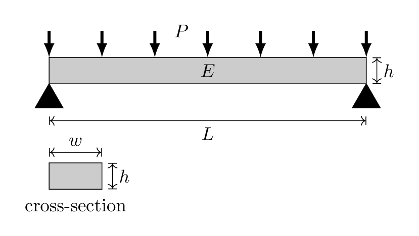
(a) Simply supported beam under uniform load.

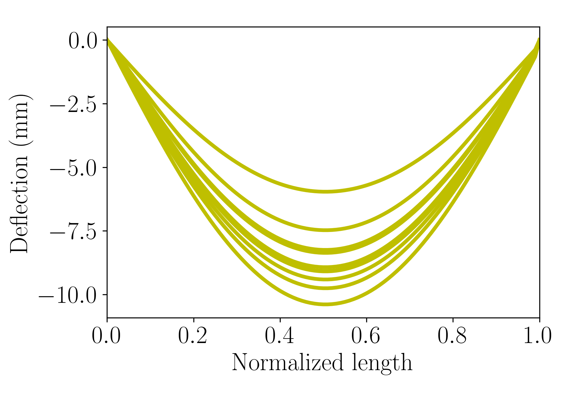
(b) Deflection over normalized beam length.

Figure 1: (a) Sketch of the simply supported beam model. (b) Beam deflection for $10$ realizations of the simply supported beam model parameters.

Table 1: Parameters of the simply supported beam model. All parameters follow a log-normal distribution with the given values for mean and standard deviation.

Parameter	Units	Notation	Mean	St. dev.
Width	m	$w$	$0.15$	$0.0075$
Height	m	$h$	$0.3$	$0.015$
Length	m	$L$	$5$	$0.05$
Young’s modulus	Pa	$E$	$3\cdot 10^{10}$	$4.5\cdot 10^{9}$
Load	N/m	$P$	$10^{4}$	$2\cdot 10^{3}$

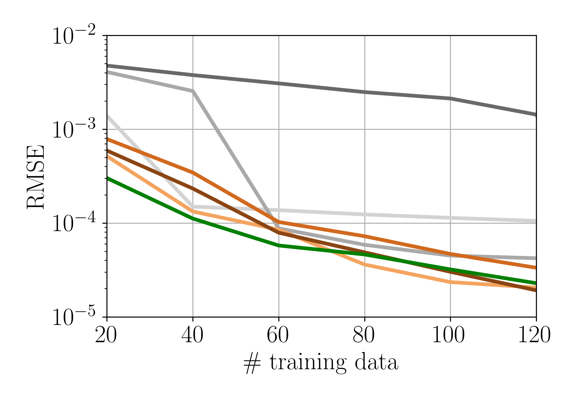
(a) RMSE, $M=500$.

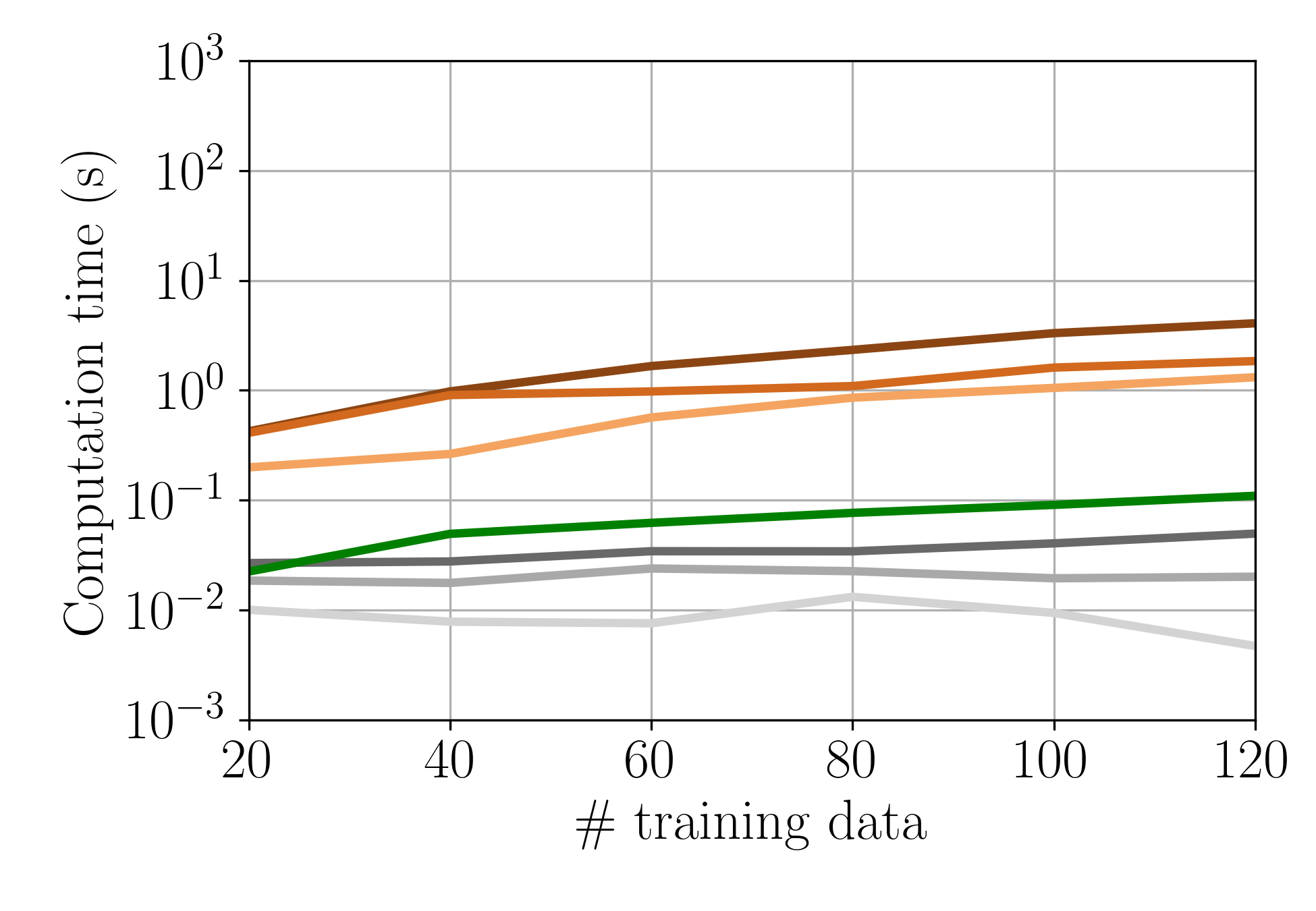
(b) Computation time, $M=10$.

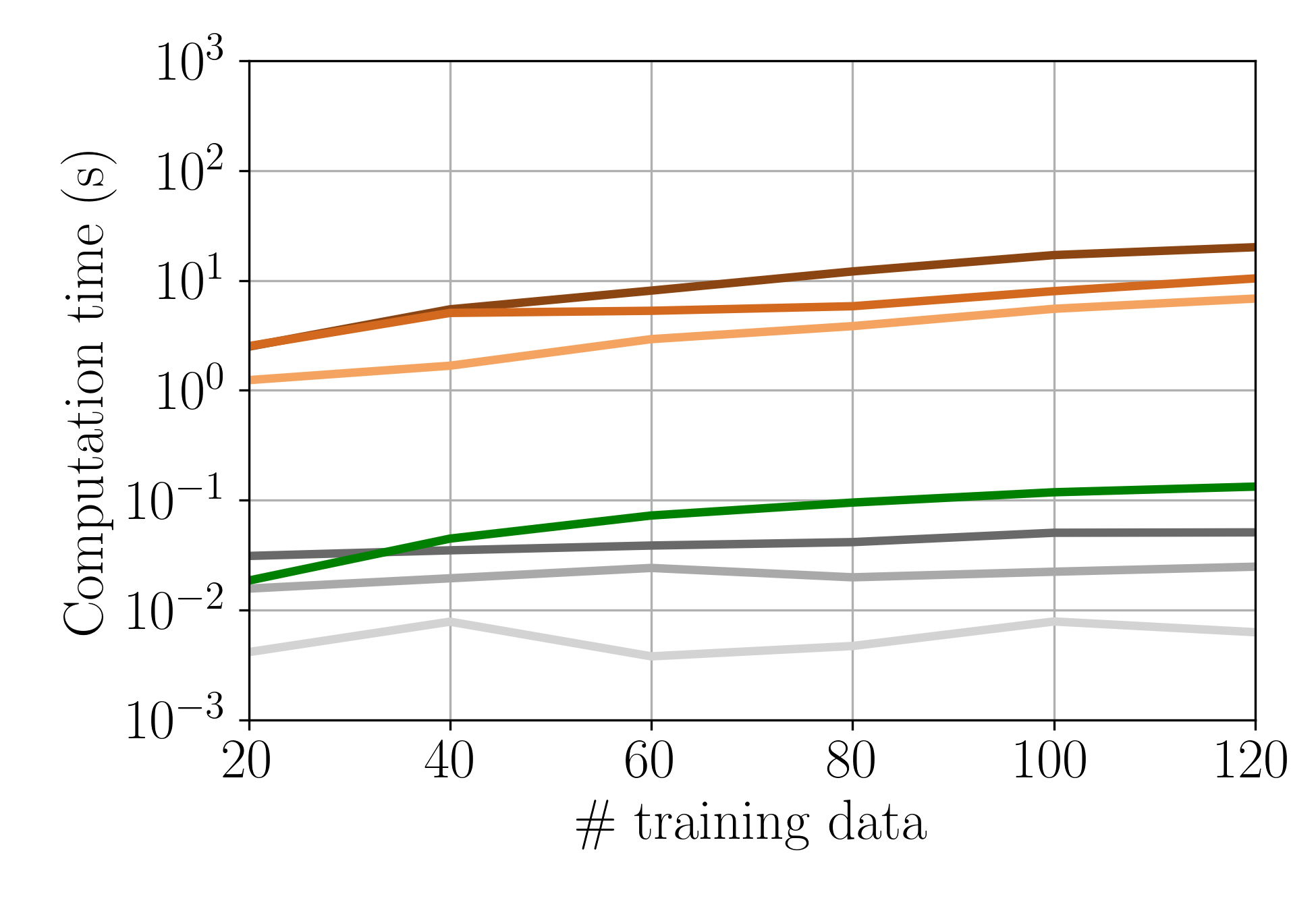
(c) Computation time, $M=50$.

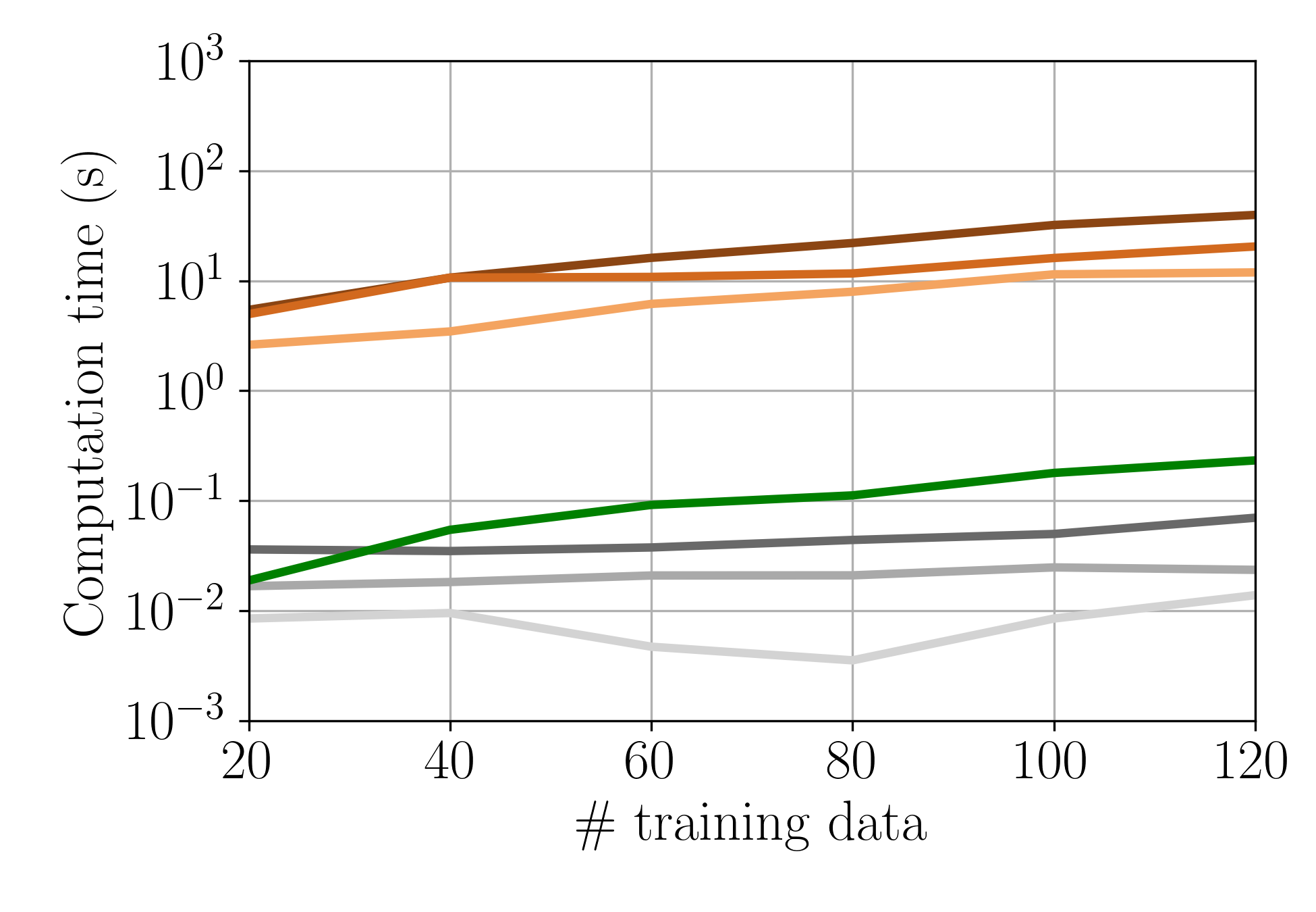
(d) Computation time, $M=100$.

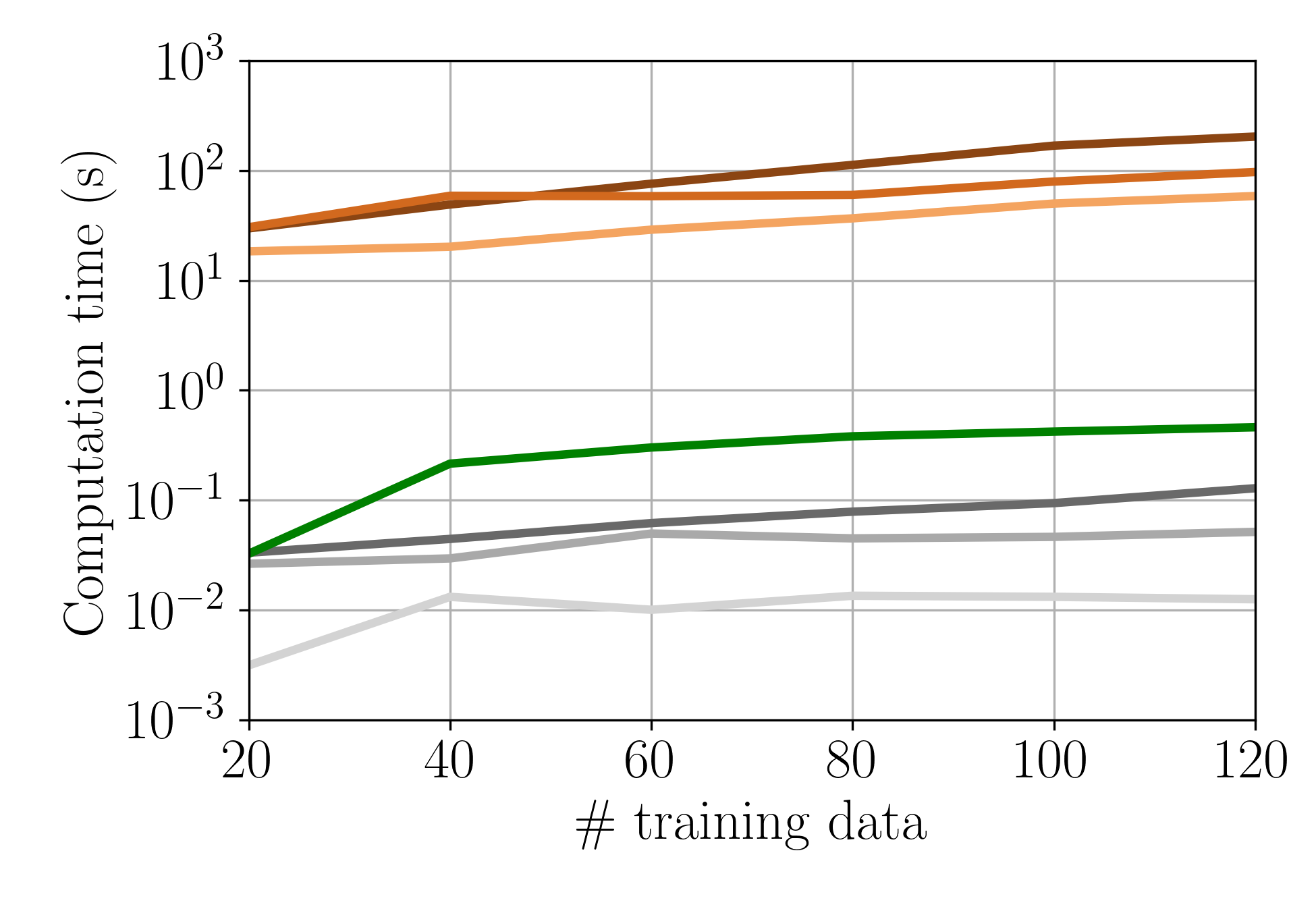
(e) Computation time, $M=500$.

Figure 2: Simply supported beam: PCE accuracy and computation time for increasing training data set size $Q\in\left[20,120\right]$ and response dimension $M\in\left\{10,50,100,500\right\}$. RMSE results only for the maximum response dimension are shown, as the rest are almost identical.

With this simple toy problem, our main goal is to assess the applicability of the competing PCE methods as the dimension $M$ of the model’s response increases. Four different response dimensions are considered, i.e., $M\in\left\{10,50,100,500\right\}$. The size of the training data set also progressively increases, such that $Q=20,40,\dots,120$.

All results with respect to accuracy and computation time for the considered PCE methods are presented in Figure 2. As expected, there is a trade-off between approximation accuracy and computation time when using adaptive and/or sparse PCEs. That is, at the cost of elevated computation times, the MVSA and the $p/q$ adaptive sparse PCE methods are generally more accurate than the fixed-basis, total degree PCEs. Nonetheless, constructing the PCE with the MVSA algorithm is orders of magnitude faster than using the $p/q$ adaptive sparse PCE methods. Moreover, the difference in computation time becomes more pronounced as the response dimension increases. At the same time, the MVSA PCE is on par with the $p/q$ adaptive sparse PCEs in terms of approximation accuracy. For example, considering the case of response dimension $M=500$ and training data set size $Q=120$, the MVSA PCE is computed in less than $0.5\,\mathrm{s}$ and yields an RMSE of $2.3\cdot 10^{-5}$. In comparison, using the $p/q$ adaptive sparse PCE methods, the computation times are 58 $\mathrm{s}$ for LAR, $97\,\mathrm{s}$ for OMP, and $204\,\mathrm{s}$ for SP, with corresponding RMSE values of $2.0\cdot 10^{-5}$, $3.3\cdot 10^{-5}$, and $1.9\cdot 10^{-5}$. That is, for a similar accuracy, the MVSA PCE is computed more than $\times 1000$ faster at minimum and more than $\times 4000$ faster at maximum.

6.2 Reflection coefficient of a rectangular waveguide

As second test case, we consider the model of a rectangular waveguide with a dielectric material filling. A two-dimensional view of the waveguide in the $xz$-plane is shown in Figure 3(a). The waveguide has width $w$ and height $h$, where the latter extends along the $y$-dimension and is therefore not shown in Figure 3(a). The dielectric filling has length $\ell$ and is separated from the waveguide’s input and output ports, respectively denoted as $\Gamma_{\mathrm{in}}$ and $\Gamma_{\mathrm{out}}$, by a vacuum offset of length $d$. The walls of the waveguide are assumed to be perfect electric conductors and are denoted with $\Gamma_{\mathrm{PEC}}$. The permittivity of the dielectric material is $\varepsilon=\varepsilon_{0}\varepsilon_{\mathrm{r}}$, where $\varepsilon_{0}$ is the permittivity in vacuum and $\varepsilon_{\mathrm{r}}$ the relative permittivity. The permeability of the dielectric material is similarly given as $\mu=\mu_{0}\mu_{\mathrm{r}}$. The relative permittivity $\varepsilon_{\mathrm{r}}$ and permeability $\mu_{\mathrm{r}}$ are given by the second-order Debye relaxation models

$$\varepsilon_{\mathrm{r}} =\varepsilon_{\infty}+\frac{\varepsilon_{\mathrm{s},1}-\varepsilon_{\infty}}{1+\iota\omega\tau_{\varepsilon,1}}+\frac{\varepsilon_{\mathrm{s},2}-\varepsilon_{\infty}}{1+\iota\omega\tau_{\varepsilon,2}}$$ (28)

$$\mu_{\mathrm{r}} =\mu_{\infty}+\frac{\mu_{\mathrm{s},1}-\mu_{\infty}}{1+\iota\omega\tau_{\mu,1}}+\frac{\mu_{\mathrm{s},2}-\mu_{\infty}}{1+\iota\omega\tau_{\mu,2}},$$ (29)

where $\omega=2\pi f$ is the angular frequency for frequency $f$, $\iota$ denotes the imaginary unit, $\varepsilon_{\infty}$ and $\mu_{\infty}$ are high-frequency relative permittivity values, $\varepsilon_{\mathrm{s},1}$, $\varepsilon_{\mathrm{s},2}$, $\mu_{\mathrm{s},1}$, and $\mu_{\mathrm{s},2}$ are static relative permittivity values, and $\tau_{\varepsilon,1}$, $\tau_{\varepsilon,2}$, $\tau_{\mu,1}$, and $\tau_{\mu,2}$ are relaxation times specific to the dielectric medium. All geometrical and material parameters of the waveguide model are listed in Table 2 along with their nominal values. The waveguide is assumed to operate within the frequency range $\left[6,30\right]\,\mathrm{GHz}$. The considered frequency dependent response is the reflection coefficient at the input port $\Gamma_{\text{\text{in}}}$, defined as $\left|\mathbf{E}_{\Gamma_{\text{in}}^{-}}/\mathbf{E}_{\Gamma_{\text{in}}^{+}}\right|$, where $\mathbf{E}$ denotes the electric field. For this simple waveguide model, the reflection coefficient can be computed semi-analytically [65, Appendix A].

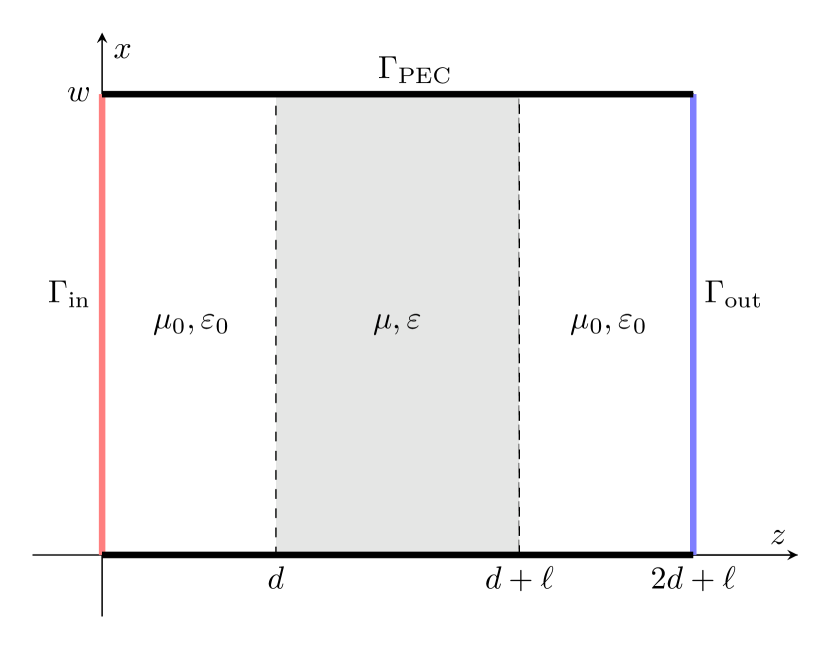
(a) Rectangular waveguide with dielectric material filling, $xz$-plane view.

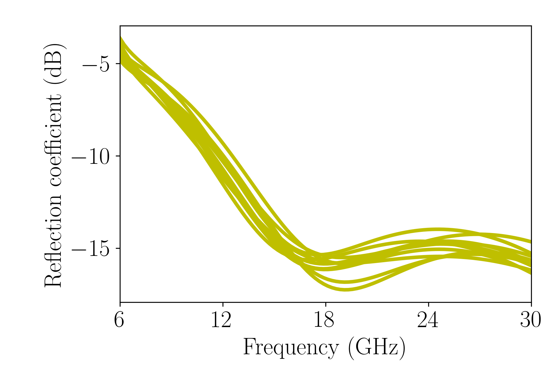
(b) Reflection coefficient over frequency range.

Figure 3: (a) View of the rectangular waveguide in the $xz$-plane. The input and output ports are shown in red and blue, respectively, the PEC walls in black, the dielectric material in gray, and vacuum in white. (b) Reflection coefficient over frequency range for $10$ realizations of the waveguide model parameters.

Table 2: Parameters of the rectangular waveguide model. Each parameter is assumed to vary uniformly within the range $\left[0.95\,\bar{x},1.05\,\bar{x}\right]$, where $\bar{x}$ denotes the nominal parameter value.

Parameter	Units	Notation	Nominal value
Width	mm	$w$	$30$
Height	mm	$h$	$3$
Dielectric filling length	mm	$\ell$	$7$
Vacuum offset length	mm	$d$	$10$
Static relative permittivity, 1st order	–	${\varepsilon}_{\text{s},1}$	$2$
Static relative permittivity, 2nd order	–	${\varepsilon}_{\text{s},2}$	$2.2$
High-frequency relative permittivity	–	${\varepsilon}_{\infty}$	$1$
Static relative permeability, 1st order	–	${\mu}_{\text{s},1}$	$2$
Static relative permeability, 2nd order	–	${\mu}_{\text{s},2}$	$3$
High-frequency relative permeability	–	${\mu}_{\infty}$	$1$
Permittivity relaxation time, 1st order	ns	${\tau}_{\varepsilon,1}$	$1/\left(40\pi\right)$
Permittivity relaxation time, 2nd order	ns	${\tau}_{\varepsilon,2}$	$1.1/\left(40\pi\right)$
Permeability relaxation time, 1st order	ns	${\tau}_{\mu,1}$	$1/\left(40\pi\right)$
Permeability relaxation time, 2nd order	ns	${\tau}_{\mu,2}$	$2/\left(40\pi\right)$

The $14$ geometrical and material parameters listed in Table 2 are allowed to vary uniformly within a $\pm 5\%$ interval centered around their nominal values, thus resulting in variations in the reflection coefficient as well. Figure 3(b) shows the reflection coefficient (in decibels) over the frequency range for different parameter realizations. Similar to Section 6.1, our goal is to assess the applicability of the considered PCE methods for an increasing response dimension $M\in\left\{10,50,100\right\}$, i.e., for an increasing number of frequency points within the frequency range, this time for a model with higher input dimensionality. The training data set size in this case ranges from $Q=50$ to $Q=500$ data points.

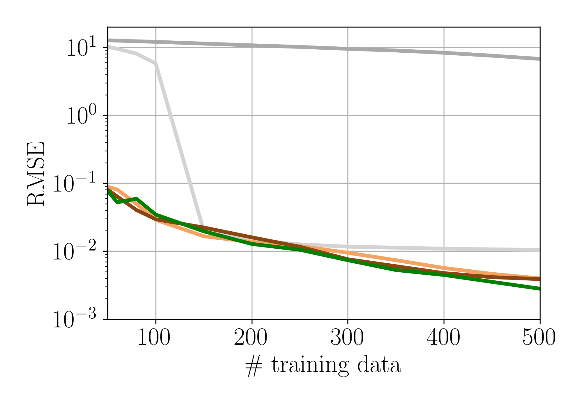
(a) RMSE, $M=100$.

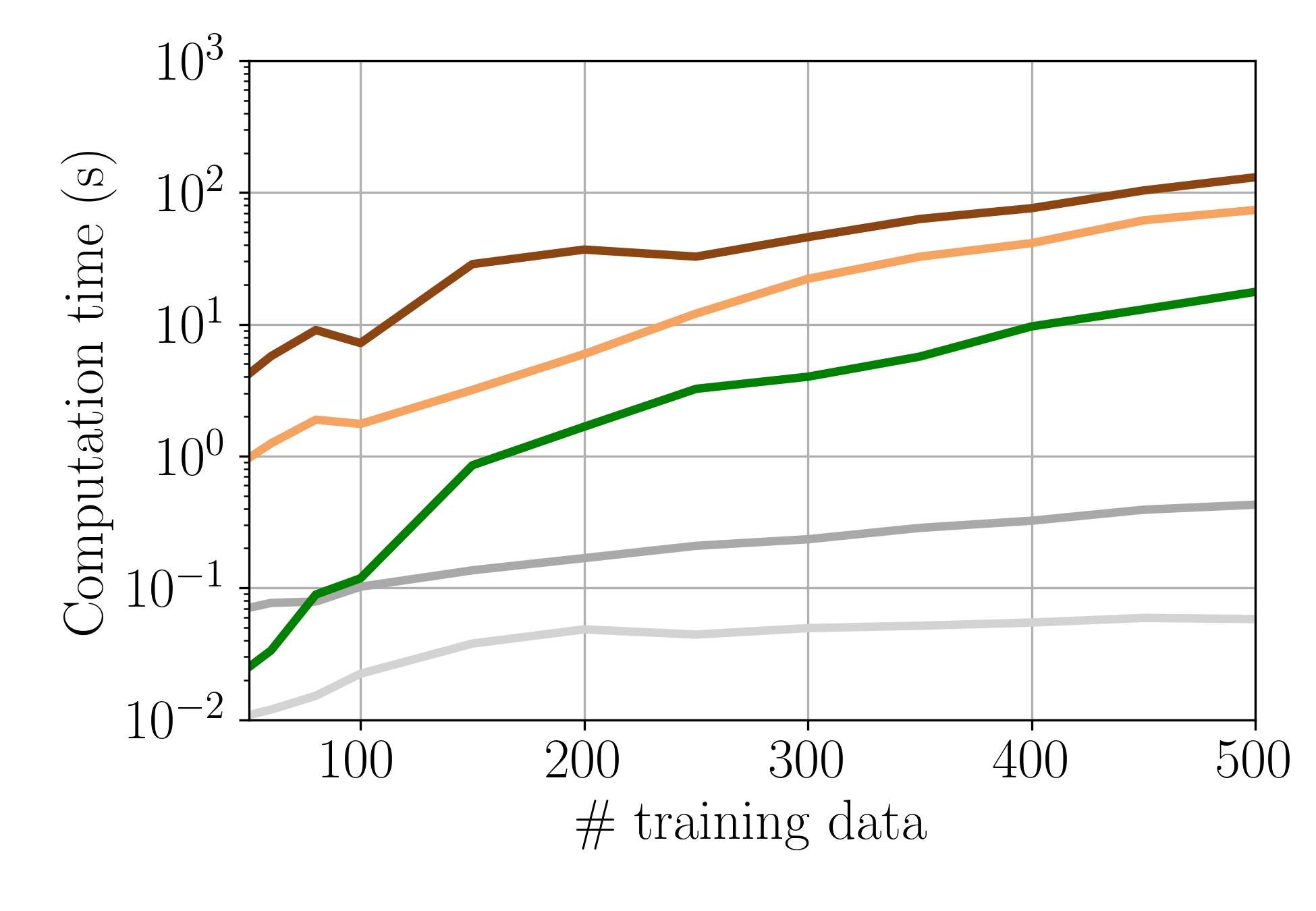
(b) Computation time, $M=10$.

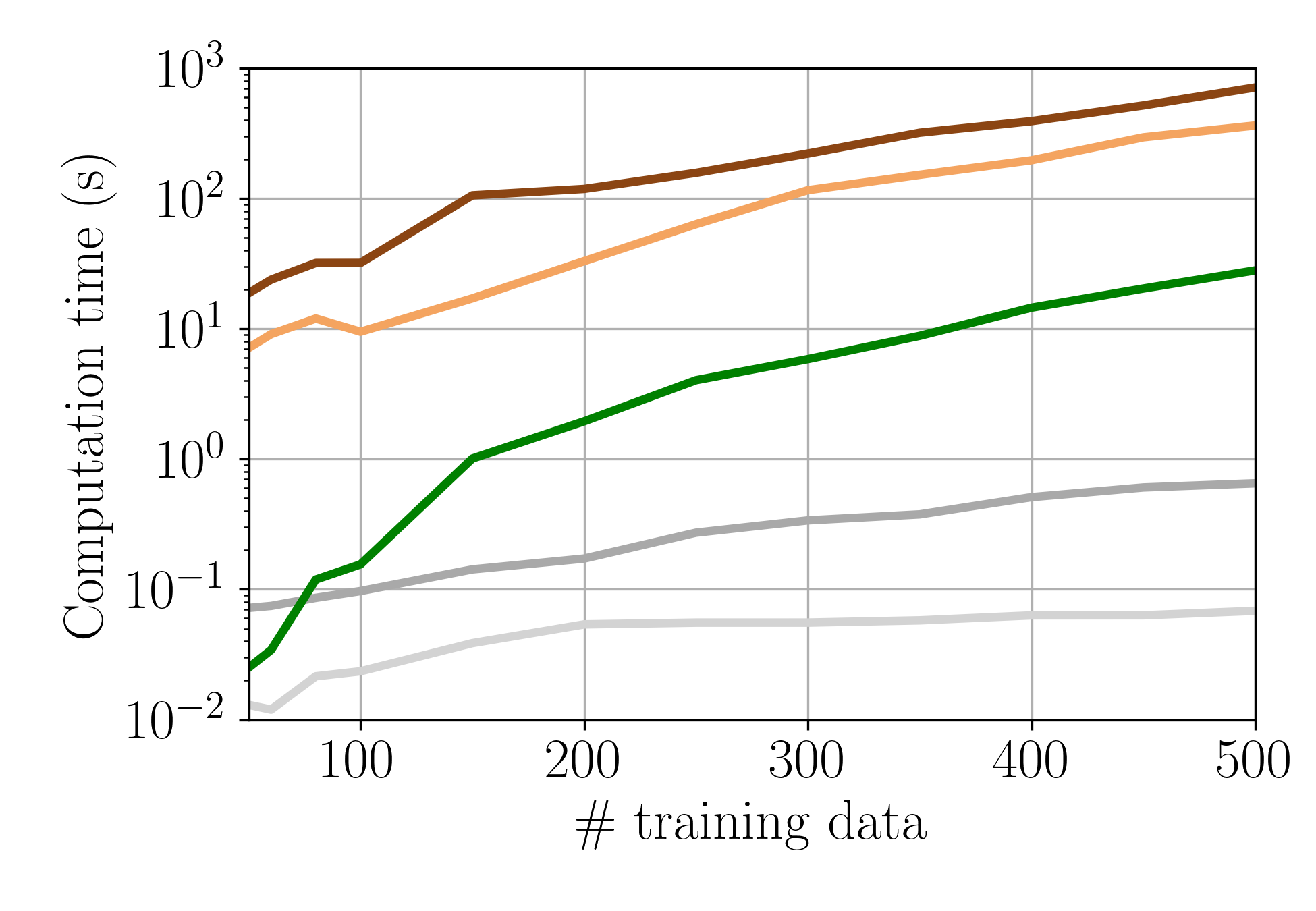
(c) Computation time, $M=50$.

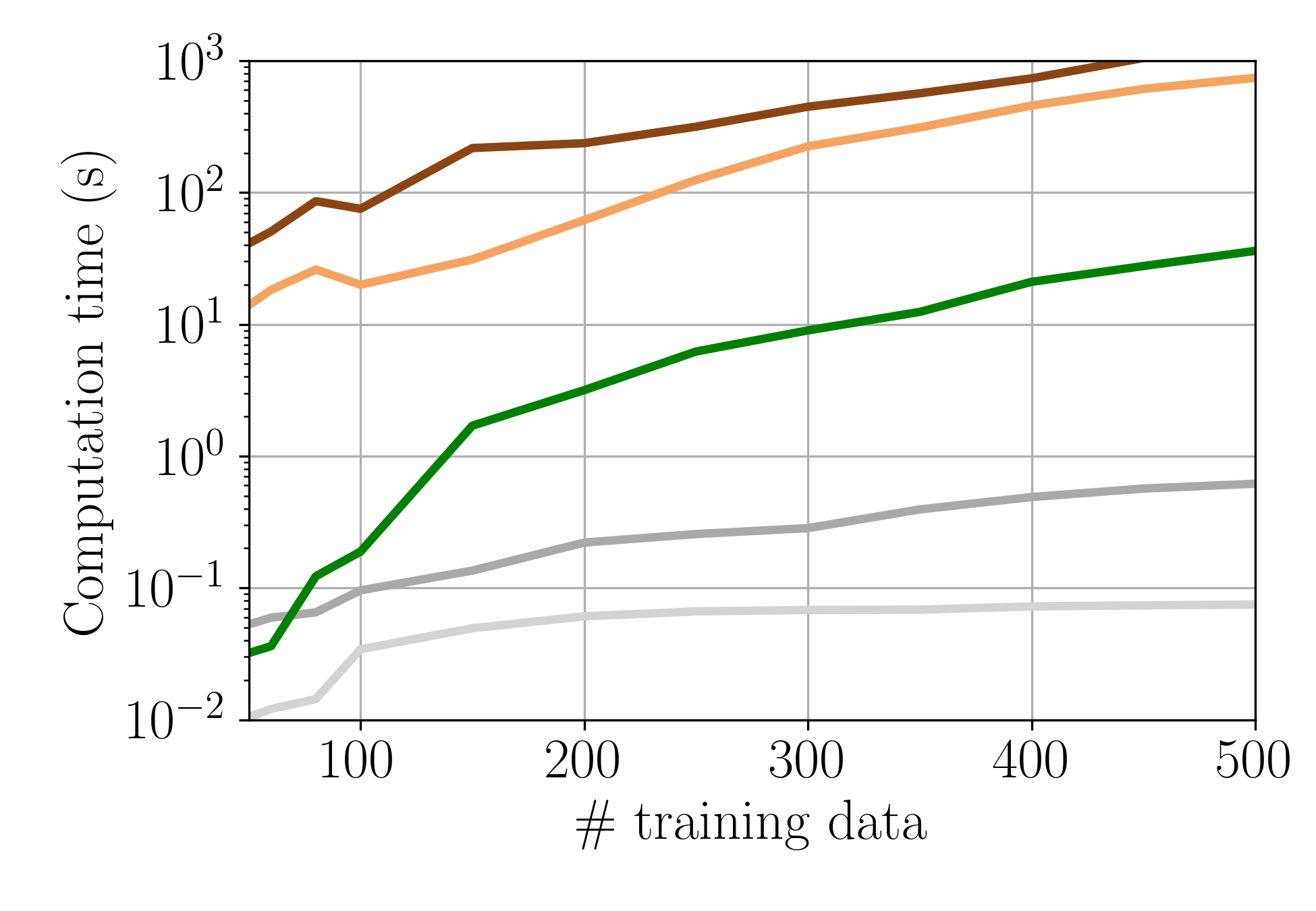
(d) Computation time, $M=100$.

Figure 4: Rectangular waveguide with dielectric filling: PCE accuracy and computation time for increasing training data set size $Q\in\left[50,500\right]$, and response dimension $M\in\left\{10,50,100\right\}$. RMSE results only for the maximum response dimension are shown, as the rest are almost identical.

The results regarding approximation accuracy and computation time for the employed PCE methods are shown in Figure 4. Due to the high dimensional input of $14$ parameters, total degree PCEs with a maximum polynomial degree $p>2$ do not offer any improvement in terms of accuracy for the given training data set sizes. The MVSA and $p/q$ adaptive sparse PCEs are more accurate, at the cost of elevated computation times. In this test case, the computation times are significantly increased due to both the high dimensional input parameter vector and, predominantly, the larger training data sets. Note that $p/q$ adaptive OMP PCE has been omitted, as it results in too high computation times even for the lowest response dimension of $M=10$. The MVSA PCE remains significantly faster than the two $p/q$ adaptive sparse PCEs, while again offering a very similar approximation accuracy. For response dimension $M=10$, the MVSA PCE is computed $\times 4$ and $\times 7$ faster than the $p/q$ adaptive LAR and SP PCEs, respectively. For $M=100$, the difference in computation time increases to $\times 20$ and $\times 41$, respectively. In fact, the computation times of the $p/q$ adaptive sparse PCEs for response dimension $M=10$ are greater than using the MVSA PCE to approximate the reflection coefficient at $M=500$ frequency points.

6.3 Torque of an induction motor

As third test case, we consider an induction motor connected to a power grid and to a mechanical load. The power grid has line-voltage amplitude equal to $V=420$ V and frequency $f=50$ Hz. The motor consists of a stator, where a winding is organized in three phases and $n_{\mathrm{pp}}=2$ pole pairs, and a rotor that rotates at the mechanical speed $\omega_{\mathrm{me}}$. The torque of the load is given by

$$T_{\mathrm{ld}}\left(\omega_{\mathrm{me}}\right)=\mathrm{sign}\left(\omega_{\mathrm{me}}\right)\left(\gamma\omega_{\mathrm{me}}^{2}+\beta\left|\omega_{\mathrm{me}}\right|+\alpha\right),$$ (30)

where the coefficients $\alpha$, $\beta$, and $\gamma$ are used for modeling static, sliding, and air friction, respectively. The mechanical equation of motion then reads

$$\frac{\mathrm{d}\omega_{\mathrm{me}}}{\mathrm{d}t}=\frac{T_{\mathrm{em}}-T_{\mathrm{ld}}\left(\omega_{\mathrm{me}}\right)}{J_{\mathrm{rt}}+J_{\mathrm{ld}}},$$ (31)

where $J_{\mathrm{rt}}$ and $J_{\mathrm{ld}}$ denote the moment of inertia of the rotor and the load, respectively, and $T_{\mathrm{em}}$ is the electromagnetic torque. Using the per-phase equivalent circuit model of the motor depicted in Figure 5(a), the electromagnetic torque is given by

$$T_{\mathrm{em}}=\frac{3R_{\mathrm{rt}}\left|I_{\mathrm{rt}}\right|^{2}}{\omega_{\mathrm{syn}}-\omega_{\mathrm{me}}},$$ (32)

where $\omega_{\mathrm{syn}}=2\pi f/n_{\mathrm{pp}}$ is the synchronous speed of the electromagnetic field generated by the stator winding within the air gap of the motor. The rotor resistance $R_{\mathrm{rt}}$ is assumed to be known, while the rotor current $I_{\mathrm{rt}}$ can be derived from the equivalent circuit’s voltage and current equations [66].

(a) Equivalent circuit of induction motor.

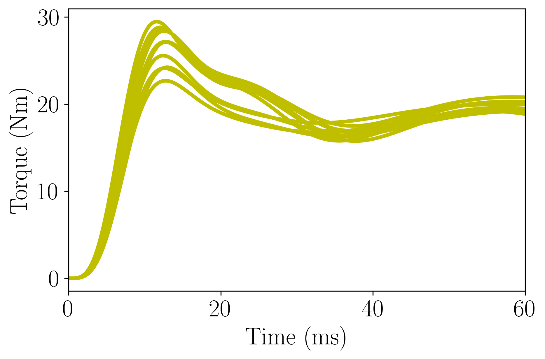
(b) Electromagnetic torque during motor start-up.

Figure 5: (a) Equivalent circuit model of an induction motor. (b) Electromagnetic torque generated during the start-up of the induction motor for $10$ realizations of the model parameters.

Table 3: Parameters of the induction motor model. The line-voltage amplitude varies uniformly within $\left[90\%,100\%\right]$ of its nominal value. The frequency varies uniformly within $\left[49.5,50.5\right]$ Hz. The remaining parameters follow normal distributions with mean equal to the nominal value and standard deviation equal to $5\%$ of the nominal value.

Parameter	Units	Notation	Nominal value
Stator resistance	$\Omega$	$R_{\mathrm{st}}$	$1.355$
Rotor resistance	$\Omega$	$R_{\mathrm{rt}}$	$2.9338$
Magnetization inductance	H	$L_{\mathrm{m}}$	$143.75\cdot 10^{-3}$
Stator leakage inductance	H	$L_{\sigma,\mathrm{st}}$	$5.87\cdot 10^{-3}$
Rotor leakage inductance	H	$L_{\sigma,\mathrm{rt}}$	$5.87\cdot 10^{-3}$
Moment of inertia of rotor	kg m2	$J_{\mathrm{rt}}$	$1.1\cdot 10^{-3}$
Moment of inertia of load	kg m2	$J_{\mathrm{ld}}$	$10^{-3}$
Constant load torque coefficient	N m	$\alpha$	$10^{-3}$
Linear load torque coefficient	N m s	$\beta$	$10^{-3}$
Quadratic load torque coefficient	N m s2	$\gamma$	$10^{-3}$
Line-voltage amplitude	V	$V$	$420$
Frequency	Hz	$f$	$50$

To simulate the start-up phase of the induction machine, where the rotor is initially at standstill ($\omega_{\mathrm{me}}=0$), the mechanical equation of motion (31) is coupled to the electrical ordinary differential equation

$$v(t)=Ri(t)+L\frac{\mathrm{d}i(t)}{\mathrm{d}t},$$ (33)

which is derived separately for the three phases in the stator and the rotor, thus resulting in a system of 6 equations [66]. The simulation model is implemented using the gym-motor software [67] and comprises the 12 input parameters described in Table 3. The line-voltage amplitude and the frequency vary uniformly within standard safety specification ranges, while all other parameters follow normal distributions with mean equal to their nominal value and standard deviation equal to $5\%$ of the nominal value. Figure 5(b) shows the electromagnetic torque of the induction motor for different parameter realizations, where each torque trajectory contains $6000$ time steps. For the considered variations, the torque trajectories can be reconstructed with almost no loss of information by using principal component analysis (PCA) and retaining $10$ principal components.

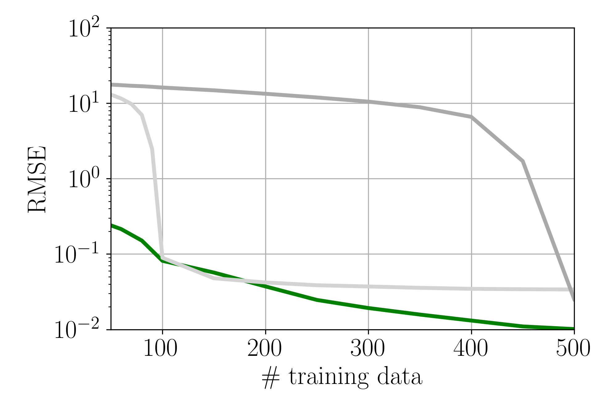
(a) RMSE, full response ($M=6000$).

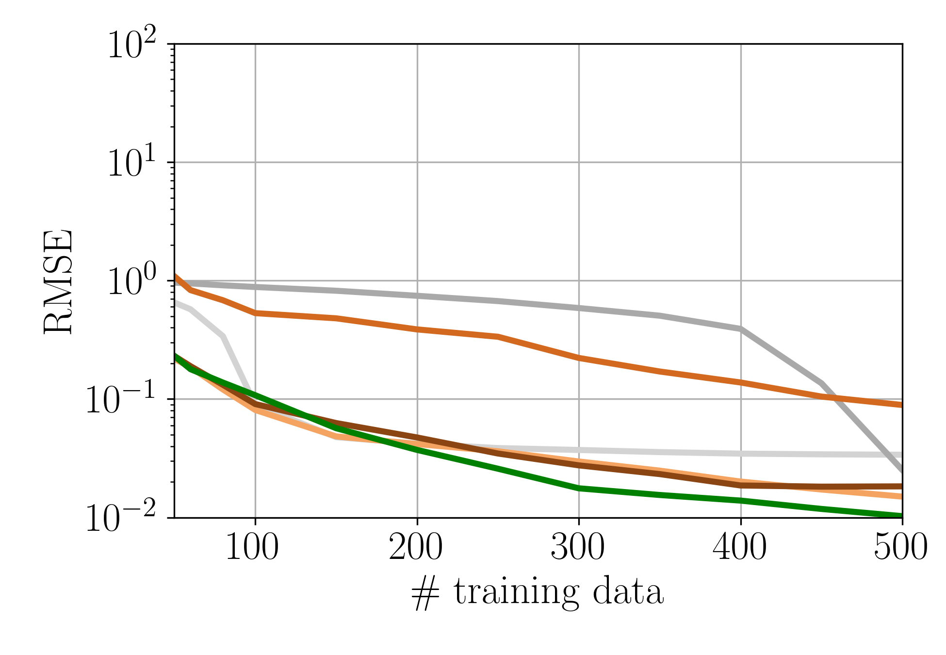
(b) RMSE, reduced response ($M=10$).

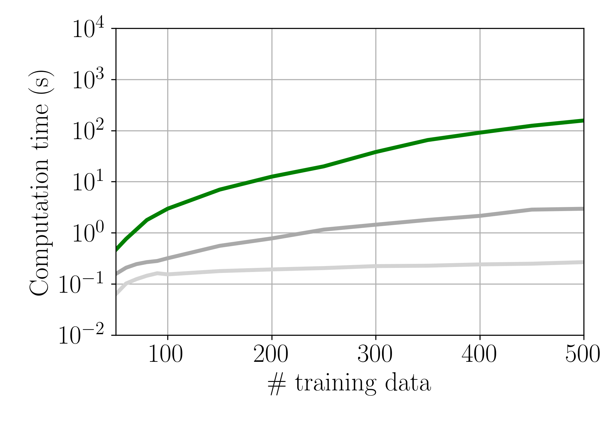
(c) Computation time, full response ($M=6000$).

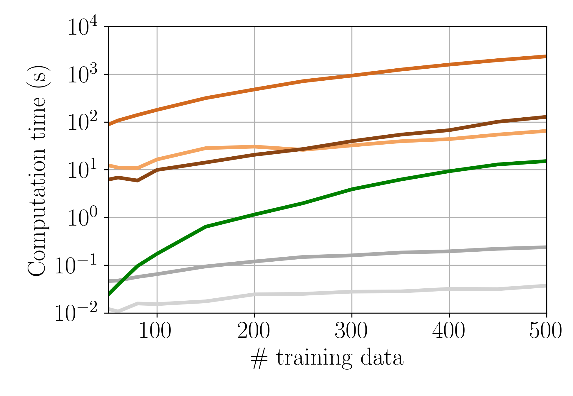
(d) Computation time, reduced response ($M=10$).

Figure 6: Induction motor: PCE accuracy and computation time for increasing training data set size $Q\in\left[50,500\right]$. The dimension of the full response is $M=6000$. By means of PCA, the reduced dimension of the response is $M=10$.

Figure 6 shows the PCE accuracy and computation time results, considering both the full model response with dimension $M=6000$ and the reduced dimension $M=10$, for training data set sizes between $Q=50$ and $Q=500$. First, looking at the full response, the $p/q$ adaptive sparse PCE methods are simply unusable, due to too long computation times. Total degree PCEs are computed almost instantaneously, but suffer from reduced accuracy. The MVSA PCE results in a comparatively high but still acceptable computation time, while providing the best approximation accuracy. Dimension reduction by means of PCA renders the $p/q$ adaptive sparse PCE methods tractable. However, the OMP solver results in poor approximation accuracy and a very large computation time. The MVSA PCE offers similar, if not slightly superior approximation accuracy to the $p/q$ adaptive LAR and SP PCEs, while also being computed $\times 3$ faster at minimum. Interestingly, the use of PCA results in an increase in the approximation accuracy of the total degree PCEs for smaller training data sets, which however remain inferior to the other methods.

7 Conclusion

This work presented a novel basis adaptive method for the construction of polynomial chaos expansions (PCEs) of multidimensional model responses. The corresponding algorithm is called multivariate sensitivity adaptive (MVSA), based on the fact the adaptive basis selection criterion makes use of variance based multivariate sensitivity analysis metrics [37, 39]. The MVSA PCE method addresses problems related to both input and output dimensionality, simultaneously. It is applicable to problems with up to moderately high dimensional model inputs, similar to previously suggested sparse and/or adaptive PCE algorithms [13, 14]. At the same time, it can be applied to approximate model responses with sizes in the order of thousands. In the latter case, the available sparse and/or adaptive PCE methods can be employed only if combined with dimension reduction methods [31, 32, 33, 34, 35].

The numerical results presented in Section 6 illustrate clearly the advantages of the proposed MVSA PCE method over competing approaches. For all considered test cases, the MVSA PCE method results in comparable or superior approximation accuracy, while at the same time being significantly more efficient concerning computation time, compared to sparse/adaptive PCE methods available in the literature. Particularly concerning the computation time of the PCE, the advantage of the MVSA algorithm becomes increasingly more prominent as the dimension of the response increases. In fact, the MVSA PCE method remains applicable for response dimensions in the order of thousands, in which case the competing sparse/adaptive PCE methods are simply unusable. However, even for a reduced output dimensionality, e.g., after the application of a dimension reduction method like principal component analysis (PCA), the MVSA PCE method is either on par or superior to the competing PCE methods in terms of approximation accuracy and again much more advantageous in terms of computation time.

The MVSA PCE method presented in this work can already be a useful surrogate modeling tool in its current form. Nonetheless, we can identify possible developments which could enhance its capabilities. For example, a multi-element extension of the method would address problems of reduced regularity [60]. On a different path, physical constraints could be incorporated during the training of the PCE, in order to depart from the pure data-driven setting and move towards a physically conforming method [68]. Last, in an effort to further reduce data demand, the multivariate sensitivity analysis metrics that have been used to guide the basis adaptivity procedure within the MVSA PCE method, can also be used to develop optimal experimental design and active learning techniques that target vector valued model responses, similar to existing methods for scalar outputs [69]. In combination with the MVSA PCE method presented in this paper, the latter could result in a basis and sampling adaptive vector valued PCE method, thus extending existing approaches [25, 24, 21] from scalar to multidimensional model responses.

References

- [1] D. Shen, H. Wu, B. Xia, D. Gan, Polynomial chaos expansion for parametric problems in engineering systems: A review, IEEE Systems Journal 14 (3) (2020) 4500–4514.
- [2] H. Lim, L. Manuel, Distribution-free polynomial chaos expansion surrogate models for efficient structural reliability analysis, Reliability Engineering & System Safety 205 (2021) 107256.
- [3] D. Loukrezis, H. De Gersem, Power module heat sink design optimization with ensembles of data-driven polynomial chaos surrogate models, e-Prime-Advances in Electrical Engineering, Electronics and Energy 2 (2022) 100059.
- [4] A. Suryawanshi, D. Ghosh, Reliability based optimization in aeroelastic stability problems using polynomial chaos based metamodels, Structural and Multidisciplinary Optimization 53 (2016) 1069–1080.
- [5] A. Thelen, X. Zhang, O. Fink, Y. Lu, S. Ghosh, B. D. Youn, M. D. Todd, S. Mahadevan, C. Hu, Z. Hu, A comprehensive review of digital twin—part 1: modeling and twinning enabling technologies, Structural and Multidisciplinary Optimization 65 (12) (2022) 354.
- [6] T. Crestaux, O. Le Maıtre, J.-M. Martinez, Polynomial chaos expansion for sensitivity analysis, Reliability Engineering & System Safety 94 (7) (2009) 1161–1172.
- [7] O. M. Knio, O. Le Maitre, Uncertainty propagation in CFD using polynomial chaos decomposition, Fluid Dynamics Research 38 (9) (2006) 616.
- [8] B. Sudret, Global sensitivity analysis using polynomial chaos expansions, Reliability engineering & system safety 93 (7) (2008) 964–979.
- [9] K. Cheng, Z. Lu, Sparse polynomial chaos expansion based on D-MORPH regression, Applied Mathematics and Computation 323 (2018) 17–30.
- [10] M. Hadigol, A. Doostan, Least squares polynomial chaos expansion: A review of sampling strategies, Computer Methods in Applied Mechanics and Engineering 332 (2018) 382–407.
- [11] G. Migliorati, F. Nobile, E. Von Schwerin, R. Tempone, Analysis of discrete L2 projection on polynomial spaces with random evaluations, Foundations of Computational Mathematics 14 (3) (2014) 419–456.
- [12] E. Torre, S. Marelli, P. Embrechts, B. Sudret, Data-driven polynomial chaos expansion for machine learning regression, Journal of Computational Physics 388 (2019) 601–623.
- [13] N. Lüthen, S. Marelli, B. Sudret, Sparse polynomial chaos expansions: Literature survey and benchmark, SIAM/ASA Journal on Uncertainty Quantification 9 (2) (2021) 593–649.
- [14] N. Lüthen, S. Marelli, B. Sudret, Automatic selection of basis-adaptive sparse polynomial chaos expansions for engineering applications, International Journal for Uncertainty Quantification 12 (3) (2022).
- [15] G. Blatman, B. Sudret, Adaptive sparse polynomial chaos expansion based on least angle regression, Journal of Computational Physics 230 (6) (2011) 2345–2367.
- [16] J. D. Jakeman, M. S. Eldred, K. Sargsyan, Enhancing l1-minimization estimates of polynomial chaos expansions using basis selection, Journal of Computational Physics 289 (2015) 18–34.
- [17] N. Alemazkoor, H. Meidani, Divide and conquer: An incremental sparsity promoting compressive sampling approach for polynomial chaos expansions, Computer Methods in Applied Mechanics and Engineering 318 (2017) 937–956.
- [18] P. Diaz, A. Doostan, J. Hampton, Sparse polynomial chaos expansions via compressed sensing and D-optimal design, Computer Methods in Applied Mechanics and Engineering 336 (2018) 640–666.
- [19] K. Sargsyan, C. Safta, H. N. Najm, B. J. Debusschere, D. Ricciuto, P. Thornton, Dimensionality reduction for complex models via Bayesian compressive sensing, International Journal for Uncertainty Quantification 4 (1) (2014).
- [20] P. Tsilifis, X. Huan, C. Safta, K. Sargsyan, G. Lacaze, J. C. Oefelein, H. N. Najm, R. G. Ghanem, Compressive sensing adaptation for polynomial chaos expansions, Journal of Computational Physics 380 (2019) 29–47.
- [21] B.-Y. Zhang, Y.-Q. Ni, A novel sparse polynomial chaos expansion technique with high adaptiveness for surrogate modelling, Applied Mathematical Modelling 121 (2023) 562–585.
- [22] S. Abraham, M. Raisee, G. Ghorbaniasl, F. Contino, C. Lacor, A robust and efficient stepwise regression method for building sparse polynomial chaos expansions, Journal of Computational Physics 332 (2017) 461–474.
- [23] W. He, Y. Zeng, G. Li, An adaptive polynomial chaos expansion for high-dimensional reliability analysis, Structural and Multidisciplinary Optimization 62 (4) (2020) 2051–2067.
- [24] M. Thapa, S. B. Mulani, R. W. Walters, Adaptive weighted least-squares polynomial chaos expansion with basis adaptivity and sequential adaptive sampling, Computer Methods in Applied Mechanics and Engineering 360 (2020) 112759.
- [25] D. Loukrezis, A. Galetzka, H. De Gersem, Robust adaptive least squares polynomial chaos expansions in high-frequency applications, International Journal of Numerical Modelling: Electronic Networks, Devices and Fields 33 (6) (2020) e2725.
- [26] R. Ghanem, P. D. Spanos, Polynomial Chaos in Stochastic Finite Elements, Journal of Applied Mechanics 57 (1) (1990) 197–202.
- [27] C. Lataniotis, S. Marelli, B. Sudret, Extending classical surrogate modeling to high dimensions through supervised dimensionality reduction: a data-driven approach, International Journal for Uncertainty Quantification 10 (1) (2020).
- [28] K. Kontolati, D. Loukrezis, D. G. Giovanis, L. Vandanapu, M. D. Shields, A survey of unsupervised learning methods for high-dimensional uncertainty quantification in black-box-type problems, Journal of Computational Physics 464 (2022) 111313.
- [29] C. V. Mai, B. Sudret, Surrogate models for oscillatory systems using sparse polynomial chaos expansions and stochastic time warping, SIAM/ASA Journal on Uncertainty Quantification 5 (1) (2017) 540–571.
- [30] V. Yaghoubi, S. Marelli, B. Sudret, T. Abrahamsson, Sparse polynomial chaos expansions of frequency response functions using stochastic frequency transformation, Probabilistic engineering mechanics 48 (2017) 39–58.
- [31] G. Blatman, B. Sudret, Sparse polynomial chaos expansions of vector-valued response quantities, CRC Press/Balkema, 2013.
- [32] B. Bhattacharyya, E. Jacquelin, D. Brizard, Uncertainty quantification of stochastic impact dynamic oscillator using a proper orthogonal decomposition-polynomial chaos expansion technique, Journal of Vibration and Acoustics 142 (6) (2020) 061013.
- [33] E. Jacquelin, N. Baldanzini, B. Bhattacharyya, D. Brizard, M. Pierini, Random dynamical system in time domain: A POD-PC model, Mechanical Systems and Signal Processing 133 (2019) 106251.
- [34] L. Hawchar, C.-P. El Soueidy, F. Schoefs, Principal component analysis and polynomial chaos expansion for time-variant reliability problems, Reliability Engineering & System Safety 167 (2017) 406–416.
- [35] J. B. Nagel, J. Rieckermann, B. Sudret, Principal component analysis and sparse polynomial chaos expansions for global sensitivity analysis and model calibration: Application to urban drainage simulation, Reliability Engineering & System Safety 195 (2020) 106737.
- [36] K. Kontolati, D. Loukrezis, K. R. dos Santos, D. G. Giovanis, M. D. Shields, Manifold learning-based polynomial chaos expansions for high-dimensional surrogate models, International Journal for Uncertainty Quantification 12 (4) (2022).
- [37] F. Gamboa, A. Janon, T. Klein, A. Lagnoux, Sensitivity analysis for multidimensional and functional outputs, Electronic Journal of Statistics 8 (1) (2014) 575–603.
- [38] I. M. Sobol, Sensitivity estimates for nonlinear mathematical models, Math. Model. Comput. Exp 1 (4) (1993) 407–414.
- [39] O. Garcia-Cabrejo, A. Valocchi, Global sensitivity analysis for multivariate output using polynomial chaos expansion, Reliability Engineering & System Safety 126 (2014) 25–36.
- [40] X. Sun, Y. Y. Choi, J.-I. Choi, Global sensitivity analysis for multivariate outputs using polynomial chaos-based surrogate models, Applied Mathematical Modelling 82 (2020) 867–887.
- [41] A. Cohen, G. Migliorati, Multivariate approximation in downward closed polynomial spaces, Contemporary Computational Mathematics-A celebration of the 80th birthday of Ian Sloan (2018) 233–282.
- [42] A. Saltelli, M. Ratto, T. Andres, F. Campolongo, J. Cariboni, D. Gatelli, M. Saisana, S. Tarantola, Global sensitivity analysis: the primer, John Wiley & Sons, 2008.
- [43] I. M. Sobol, Global sensitivity indices for nonlinear mathematical models and their Monte Carlo estimates, Mathematics and computers in simulation 55 (1-3) (2001) 271–280.
- [44] K. Campbell, M. D. McKay, B. J. Williams, Sensitivity analysis when model outputs are functions, Reliability Engineering & System Safety 91 (10-11) (2006) 1468–1472.
- [45] M. Lamboni, D. Makowski, S. Lehuger, B. Gabrielle, H. Monod, Multivariate global sensitivity analysis for dynamic crop models, Field Crops Research 113 (3) (2009) 312–320.
- [46] M. Lamboni, H. Monod, D. Makowski, Multivariate sensitivity analysis to measure global contribution of input factors in dynamic models, Reliability Engineering & System Safety 96 (4) (2011) 450–459.
- [47] A. W. Van der Vaart, Asymptotic statistics, Vol. 3, Cambridge University Press, 2000.
- [48] N. Wiener, The homogeneous chaos, American Journal of Mathematics 60 (4) (1938) 897–936.
- [49] D. Xiu, G. E. Karniadakis, The Wiener–Askey polynomial chaos for stochastic differential equations, SIAM journal on scientific computing 24 (2) (2002) 619–644.
- [50] C. Soize, R. Ghanem, Physical systems with random uncertainties: chaos representations with arbitrary probability measure, SIAM Journal on Scientific Computing 26 (2) (2004) 395–410.
- [51] X. Wan, G. E. Karniadakis, Multi-element generalized polynomial chaos for arbitrary probability measures, SIAM Journal on Scientific Computing 28 (3) (2006) 901–928.
- [52] S. Oladyshkin, W. Nowak, Data-driven uncertainty quantification using the arbitrary polynomial chaos expansion, Reliability Engineering & System Safety 106 (2012) 179–190.
- [53] J. Feinberg, V. G. Eck, H. P. Langtangen, Multivariate polynomial chaos expansions with dependent variables, SIAM Journal on Scientific Computing 40 (1) (2018) A199–A223.
- [54] J. D. Jakeman, F. Franzelin, A. Narayan, M. Eldred, D. Plfüger, Polynomial chaos expansions for dependent random variables, Computer Methods in Applied Mechanics and Engineering 351 (2019) 643–666.
- [55] S. Rahman, A polynomial chaos expansion in dependent random variables, Journal of Mathematical Analysis and Applications 464 (1) (2018) 749–775.
- [56] P. G. Constantine, M. S. Eldred, E. T. Phipps, Sparse pseudospectral approximation method, Computer Methods in Applied Mechanics and Engineering 229 (2012) 1–12.
- [57] P. R. Conrad, Y. M. Marzouk, Adaptive Smolyak pseudospectral approximations, SIAM Journal on Scientific Computing 35 (6) (2013) A2643–A2670.
- [58] J. Winokur, D. Kim, F. Bisetti, O. P. Le Maître, O. M. Knio, Sparse pseudo spectral projection methods with directional adaptation for uncertainty quantification, Journal of Scientific Computing 68 (2) (2016) 596–623.
- [59] G. T. Buzzard, Efficient basis change for sparse-grid interpolating polynomials with application to T-cell sensitivity analysis, Computational Biology Journal 2013 (2013).
- [60] A. Galetzka, D. Loukrezis, N. Georg, H. De Gersem, U. Römer, An hp-adaptive multi-element stochastic collocation method for surrogate modeling with information re-use, International Journal for Numerical Methods in Engineering 124 (12) (2023) 2902–2930.
- [61] R. Tibshirani, Regression shrinkage and selection via the lasso, Journal of the Royal Statistical Society Series B: Statistical Methodology 58 (1) (1996) 267–288.
- [62] D. L. Donoho, Compressed sensing, IEEE Transactions on Information Theory 52 (4) (2006) 1289–1306.
- [63] S. Marelli, B. Sudret, UQLab: A framework for uncertainty quantification in Matlab, in: Vulnerability, uncertainty, and risk: quantification, mitigation, and management, 2014, pp. 2554–2563.
- [64] M. Baudin, A. Dutfoy, B. Iooss, A.-L. Popelin, OpenTURNS: An Industrial Software for Uncertainty Quantification in Simulation, Springer International Publishing, 2016, pp. 1–38.
- [65] D. Loukrezis, Adaptive approximations for high-dimensional uncertainty quantification in stochastic parametric electromagnetic field simulations, Ph.D. thesis, Technische Universität Darmstadt (2019).
- [66] J. Pyrhonen, T. Jokinen, V. Hrabovcova, Design of rotating electrical machines, John Wiley & Sons, 2013.
- [67] P. Balakrishna, G. Book, W. Kirchgässner, M. Schenke, A. Traue, O. Wallscheid, Gym-electric-motor (GEM): A python toolbox for the simulation of electric drive systems, Journal of Open Source Software 6 (58) (2021) 2498.
- [68] L. Novák, H. Sharma, M. D. Shields, Physics-informed polynomial chaos expansions, arXiv preprint arXiv:2309.01697 (2023).
- [69] L. Novák, M. Vořechovskỳ, V. Sadílek, M. D. Shields, Variance-based adaptive sequential sampling for polynomial chaos expansion, Computer Methods in Applied Mechanics and Engineering 386 (2021) 114105.